Climatic Uncertainty in the Mediterranean Basin and Its Possible Relevance to Important Economic Sectors

Laboratory of Climatology, Department of Geography and Environmental Studies, University of Haifa, Haifa 34987838, Israel
Atmosphere 2019, 10(1), 10; https://doi.org/10.3390/atmos10010010
Submission received: 28 August 2018
/
Revised: 17 December 2018
/
Accepted: 17 December 2018
/
Published: 2 January 2019
(This article belongs to the Special Issue Climate Variabilities and Changes in the Mediterranean Basin and their Impacts on Mediterranean Societies)
Abstract
:The Mediterranean Basin is among the densest populated regions of the world with forecasts for a further population increase in the coming decades. Agriculture and tourism are two main economic activities of this region. Both activities depend highly on climate and weather conditions. Climate and weather in turn, present a large variability both in space and in time which results in different uncertainty types. Any change in weather and or climate conditions in the coming decades due to climate change may increase this uncertainty. Temporal uncertainty is discussed in detail and different ways of how to exhibit it are presented with examples from various locations in the Mediterranean basin. Forecasted increased uncertainty may in turn increase future challenges for long term planning and managing of agriculture and tourism in that part of the world.
1. Introduction
The Mediterranean is the densest populated closed sea in the world. The total population of the Mediterranean countries grew from 276 million in 1970 to 412 million in 2000 and to 466 million in 2010. It is predicted to reach 529 million by 2025 [1].
The Mediterranean Basin, similar to other regions of the world, is projected to experience considerable climate changes in the next decades. Ref. [2] reviewed the projected changes based on a series of ensembles of global and regional climate change simulations. They summarized the main expected changes as a decrease in precipitation due to a northward shift of the Atlantic storm tracks, a pronounced warming and increase in intra annual variability. It should be emphasized that in most of the Mediterranean Basin there is a high or severe water stress which may increase due to increasing demands of a growing population and a decrease in rainfall [3]. These projected changes, that some are already evident, increase the challenges of decision makers in a series of fields related to the daily life in that region.
The objectives of the present study are: a-To describe the various types of uncertainties and their causes; b-To review the main characteristics of weather and climate conditions in the Mediterranean Basin; c-To demonstrate and quantify these uncertainties in various parts of the Mediterranean and d-To discuss their impacts on various activities mainly on tourism and agriculture. Nevertheless, this article is not intended to be a how to do guide for decision makers in both fields.
2. Factors Affecting Uncertainty
“Uncertainty exists where there is a lack of knowledge concerning outcomes. Uncertainty may result from an imprecise knowledge of the risk, that is, where the probabilities and magnitude of either the hazards and/or their associated consequences are uncertain. Even when there is a precise knowledge of these components there is still uncertainty because outcomes are determined probabilistically” [4].
Three main factors may determine the degree of climatic uncertainty; the natural variability of the parameter in case, the amount of available data and the selection of the appropriate scenario (Figure 1). Uncertainty increases in regions and seasons where the natural variability is greater. The uncertainty depends a great deal on the amount of available reliable data. Lack of sufficient data and/or choosing an inappropriate scenario, increases the uncertainty regarding the future behaviour of the variable in case. This is in agreement with similar claims made by [5,6]. In the present study only the natural variability and lack of sufficient data will be addressed.
One of the main characteristics of the Mediterranean climate is its large spatial and temporal variability of several climatic variables.
Three main meteorological variables (among others) are usually addressed when the climate of a certain region is analysed: Atmospheric pressure, temperature and precipitation (rainfall). These three variables however, differ in some of their characteristics such as: spatial and/or temporal continuity, spatial and/or temporal representation and the meaningfulness of measurements. Therefore, they should be analysed and presented in different ways. In the following sections these characteristics are illustrated with some examples from various regions within the Mediterranean Basin.
2.1. Spatial and/or Temporal Continuity
A variable is continuous when: having the property that the absolute value of the numerical difference between the value at a given point and the value at any point in a neighbourhood of the given point can be made as close to zero as desired by choosing the neighbourhood small enough (Merriam-Webster).
While temperature and atmospheric pressure are continuous in space and time (e.g., [7]), namely the temperature at a certain location cannot drop from say, 30 °C to 24 °C without passing through all intermediate values even when this happens rapidly. Similarly, if the atmospheric pressure is for example 1004 hPa at one location and 995 hPa at another, all intermediate values exist in between even if those two locations are close each other. Therefore, spatial and/or temporal interpolations between observations are possible, assuming continuity. Interpolation enables to estimate the magnitude of these variables at locations and/or timing between measurements.
This is not the case for rainfall which is not continuous neither in space nor in time (e.g., [8,9]). Therefore, interpolation of rainfall totals between observations should be avoided, certainly for short periods of time (hours, days, rain-spells), even though many researchers do it. Several researchers such as, refs. [10,11,12] pointed out the increasing uncertainties regarding spatial estimation of precipitation from point measurements mainly for short periods. Ref. [8] reported that a rain gauge network density should be in the order of 0.1 of the median event size in order to adequately represent the complexity of the spatial rain distribution. However, even in the UK or in Israel, two countries with the densest national networks, the average rain gauge density is in the order of 0.8–1.0 the median event size, or 8 to 10 times less dense than necessary [9]. In other countries, mainly in North Africa, networks are by far less dense. As a consequence, this discontinuity and the lack of enough point measurements increases our inability to estimate accurately the spatial and/or temporal rainfall distribution in these regions, mainly for the above mentioned short periods. Other measurement devices such as radar signals and/or satellite images have their own calibration problems or no enough coverage, which are beyond the scope of the present study. This makes the use of point measurements as the main source for an accurate estimation of the spatial rainfall distribution in many regions.
2.2. Spatial and/or Temporal Representation
Assuming meteorological measurements were made accurately, their spatial and/or temporal representation still depends on the degree of variability in space and/or time of the variable in case. Some variables may change very rapidly over a very short period of time and/or from one site to another, even very close each other. Therefore, many measurements are needed in order to represent them accurately over space and time. An example of such a variable, is wind (speed, direction and gusts). Wind properties near the surface, in turn, are one of the most important factors that affect the rainfall distribution over space and therefore, rainfall spatial representation (mainly over short periods of time) is also very limited. On the other hand, for example, upper level geopotential heights tend to vary less over space and time and thus, their spatial structure can be accurately defined based on a relatively small number of measurements.
Another important issue related to maps of average atmospheric pressure over a certain period of time, is how they should be interpreted? For example, when comparing two maps, one showing average temperature for a certain period and the other showing the average atmospheric pressure for the same period, the former (temperature) will be comparable to most daily maps, whereas the latter (atmospheric pressure or geopotential heights) will differ a great deal from each single daily map. Such an example is presented in Figure 2 and Figure 3. All maps (of both variables) are based on NCEP reanalysis daily averages.
Figure 2a, presents the average air temperature at the 1000 hPa level for the period 1 December 2017–28 February 2018. This map, which is compiled from 90 daily maps, shows a very clear temperature gradient from North Africa to southern and central Europe. Figure 2b–h show similar temperature gradients from south to north for seven sample days within the averaged period. In other words, the averaged map reflects the various daily patterns of each single day.
Figure 3a, presents the average geopotential heights at the 1000 hPa level for the same period. This map, similarly to Figure 2a, is also compiled from 90 daily maps. It shows a very shallow depression located over the Tyrrhenian Sea, Corsica and central Italy extending from north-west to south-east. However, none of the 7 sample daily maps (Figure 3b–h), nor of the remaining 83 daily maps (not shown), present any pattern resembling the average pattern. This implies that an average pressure map, unlike a temperature average map (or any other meteorological variable map) cannot serve for locating the main pressure systems during the averaged period, nor their magnitude and certainly not the derived circulation during the averaged period.
Evidently, no one will present a map showing averaged wind directions, for example, averaging easterly winds, (azimuth 90) with westerly winds, (azimuth 270) will result in southerly winds, (azimuth 180). Similarly, one should avoid doing so for pressure (or geopotential heights) like in Figure 3a. If one wishes to present the dominant circulation over a certain area, it can be displayed on a map together with the probability to obtain such a circulation. Maps like in Figure 3a should be regarded as an indicator of the probability of the presence of a depression (or a high) in the region. The only thing that one can say is that during the period 1 December 2017–28 February 2018 the largest probability for a presence of a depression in the Mediterranean Basin was in the aforementioned region of the Tyrrhenian Sea, Corsica and central Italy but nothing about their extension, depth or frequency of such depressions. This is true for any averaged pressure map anywhere around the world.
2.3. Meaningfulness of Measurements
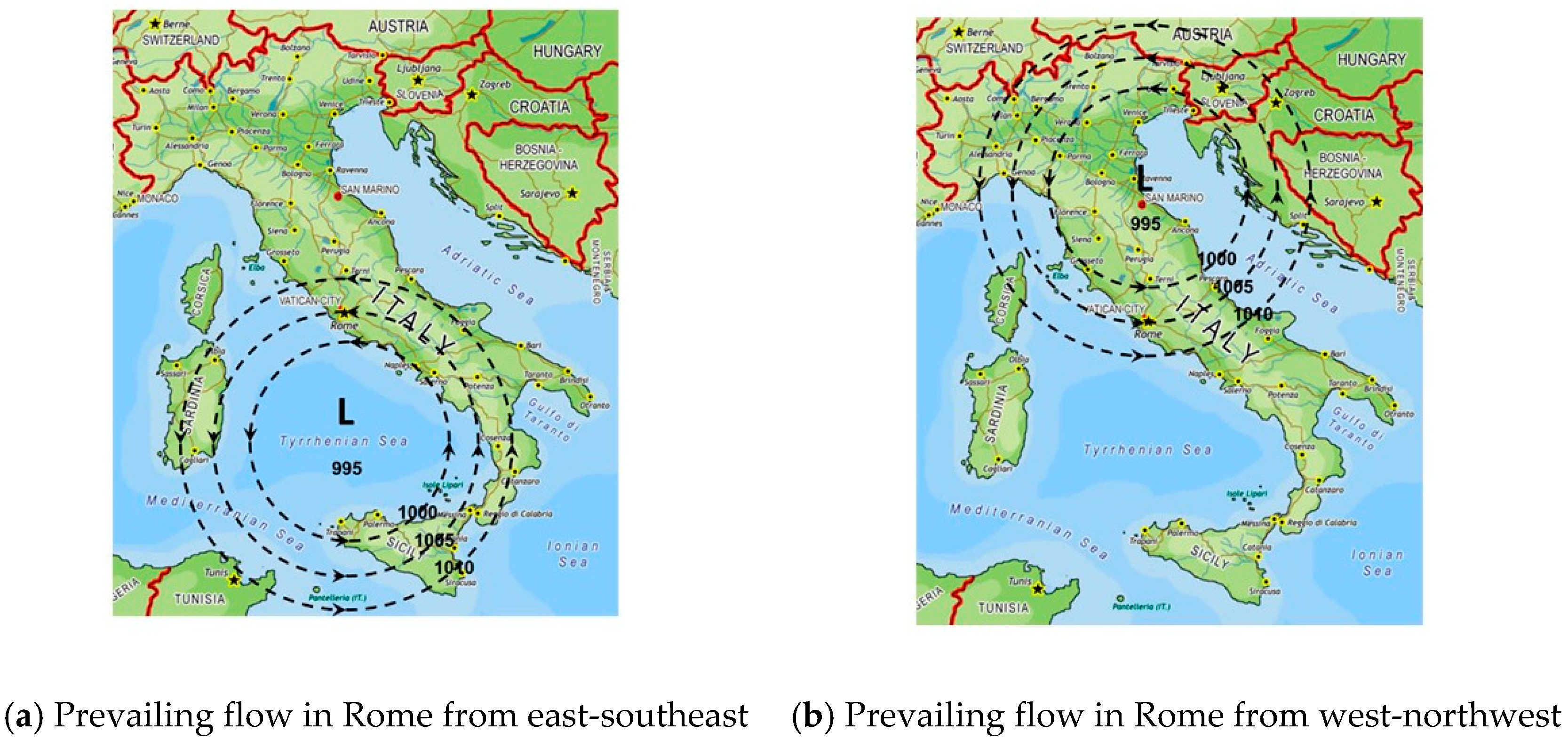
Regardless of their representation (previous paragraph), measured meteorological parameters are not always meaningful unless additional information is provided. If one is interested in the present weather conditions in, for example, Rome (or at any other location), one will look at the present air temperature, relative humidity, wind speed, wind direction, accumulated rainfall and so on, in Rome. This information will be very informative and meaningful for understanding the present weather conditions in that city. However, the present atmospheric pressure in Rome is completely meaningless unless additional information regarding the pressure in all neighbouring regions is provided. The same atmospheric pressure measured at a certain location can provide completely different weather conditions while similar conditions can occur with different pressure values. Such a schematic example is presented in Figure 4. In Figure 4a, a depression is located over southern Italy and the pressure at Rome is 1005 hPa with prevailing flow from east-southeast. In Figure 4b an identical depression in terms of size and deepness is located over northern Italy. The pressure at Rome is again 1005 hPa but this time the prevailing flow is from west-northwest causing completely different weather conditions. Thus, as postulated, atmospheric pressure at a single location without additional information is completely meaningless.
3. Types of Uncertainty
Usually, in climate or weather forecast, when referred to uncertainty, it is meant an uncertainty in the magnitude of an event, for example, how cold it will be or how intense a rain event will be and what are the probabilities for such events?
However, uncertainty refers also to When and Where a certain event may occur? For example, a snow storm which may be very likely to occur somewhere in January is very unlikely to occur at the same location, in May or a sandstorm that is frequent in North Africa may be very rare in Scandinavia.
Figure 5 presents schematically various types of uncertainties. The present article concentrates mainly (but not only) on temporal uncertainties. Temporal uncertainty itself can be divided into three major components; long-term trends, inter-annual uncertainty (variability from one year to another) and intra-annual uncertainty (variability within the year). The intra-annual uncertainty reflects uncertainty in the timing of a certain event, its duration, intensity and intervals between two consecutive events.
3.1. Intra-Annual Uncertainty
3.1.1. Uncertainty in Timing
This uncertainty (mainly regarding the rainfall) is not less crucial and maybe even more than the year-to-year variability of the annual totals especially in regions with a Mediterranean type climate having a long dry summer period.
In order to define the timing of the rainy season, one should define first the rainy season beginning date (RSBD) and rainy season ending date (RSED) and accordingly define the rainy season length (RSL):
RSL = RSED − RSBD
This issue was discussed in detail by [13,14,15]. In the Mediterranean region, the beginning of the rainy season after the long summer dryness is very sporadic. Some minute rains may occur as early as the beginning of September or even late August and then a long break with the next rain event to occur a couple of weeks or even a month later. A similar behaviour exists also at the end of the rainy season as a minute rainfall event may occur at the end of May or even at the beginning of June after many weeks of dryness. Ref. [13] reported that on average, the first 10% of the annual rainfall in Haifa were accumulated over a period of more than 5 weeks. It took on average, two months for the accumulation of the last 10% whereas, in the mid-season, 10% of the annual rainfall are accumulated in less than 2 weeks. Ref. [14] reported similar results for some inland stations in Israel and [15] for the entire Mediterranean Basin. Even if the RSBD and RSED are defined as the dates when 10% and 90% respectively, were accumulated, as suggested by [13] and modified later by [15], which is more realistic, yet their variability from year to year is enormous. The RSBD is crucial mainly for agricultural purposes (e.g., when to seed new crops) whereas, the RSED is crucial mainly for tourism activities (e.g., when to re-open or reactivate some resorts closed during the rainy season).
The intra-annual uncertainty can be measured in two ways:
- (a)
- the range of dates when a certain percentage of the annual rainfall is obtained. For example, when the mid-season date (MSD), the date when 50% of the annual rainfall was accumulated, occur.
- (b)
- the range of percentages accumulated at a certain date.
It should be made clear that both metrics can be calculated only after the end of the rainy season in case.
3.1.2. Range of Dates and Percentages
In an article on the rainfall regime in Lisbon in the last 150 years [16] it can be noticed that the intra-annual temporal variability is very large. The median MSD is January 11 (as summer is dry, the hydrological year is adopted, that is, 1 July–30 June of the next calendar year). 29 October was the earliest day when 50% of the annual rainfall were accumulated while, 18 March was the latest day, more than 4.5 months apart. If we consider the range of dates 90%–10%, this range decreases to over two months (Figure 8 in [16]).
In the same figure it can be noticed that although January 11 is the average MSD, that is, accumulation of 50% of the annual rainfall, the range of percentages accumulated on that date varies from 16.6% (January 1975) to 78.6% (January 1990). In other words, in the rainy season 1974–1975 from 1 July 1974 to 11 January 1975 only 16.6% of the annual rainfall was accumulated and from 12 January 1975 to 30 June 1975, the remaining 83.4%. On the other hand, in the rainy season 1989–1990 from 1 July 1989 to 11 January 1990, 78.6% of the annual rainfall were accumulated and from that date to the end of the season on 30 June 1990 the remaining 21.4%. The first is an example for very late-rains’ season whereas the later for very early-rains’ season.
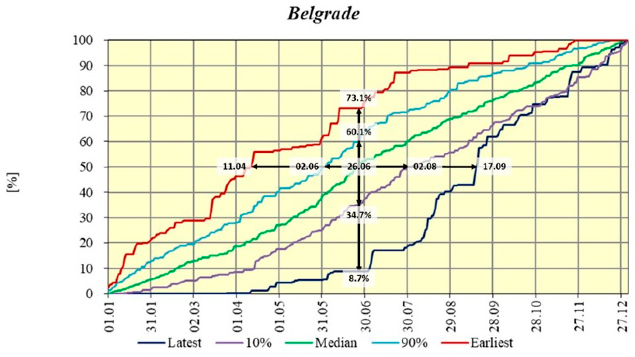
This variability is evident also in other parts of the Mediterranean Basin. Figure 6 presents the range of dates of the MSD in Belgrade. The median MSD is 26 June (unlike in Lisbon, in Belgrade rainfall occurs all year around and therefore annual rainfall is calculated from 1 January to 31 December). The earliest date when 50% where accumulated was 11 April, whereas the latest, 17 September, a range of 159 days (more than five months) for the accumulation of the same percentage of the annual rainfall. The range of dates excluding the earliest 10% and latest 10%, was two months (2 June to 2 August).
This temporal variability can be demonstrated also by comparing the accumulated percentages on the MSD. The lowest was 8.7% whereas the highest 73.1% or a range of 64.4% of the annual rainfall accumulated on the same date. While, in one year over 90% of the annual rainfall was accumulated in the second half of the year, from the end of June to the end of December, in another only a quarter of the annual rainfall was accumulated in that period. As the accumulation percentages can be calculated only after the year ends, no one knows what share of the annual rainfall was accumulated on a certain date and how much still remains. This variability demonstrated on Belgrade’s data, in which rain falls all year long, is more crucial in other parts of the Mediterranean Basin where rain occur mainly in winter and in the transitional seasons whereas, summer is dry (e.g., [16,17]).
3.1.3. Uncertainty in Duration
The duration of a climatic event sometimes determines its severity or rarity and therefore its consequences. For example, a temperature of 35 °C in one summer day at Jerusalem, is a common event, the same temperature lasting for a week will be considered as an extreme event and the consequences will be accordingly. Ref. [18] analysed the 2003 heat wave in western Europe that was the longest ever recorded in that region which caused tens of thousands of deaths in several countries [19].
Similar consequences can be attributed also to the duration of drought (see below in the “Dryness” section). Very recently [20], reported about a possible association between preceding drought occurrence and heat waves in the Mediterranean. The duration of events may have very important consequences in many aspects not only during exceptional extreme cases.
Figure 7 presents the average annual rain-spell duration (RSD) in Turkey based on daily data from 42 years (1970–2011). Figure 7a shows the shortest mean annual RSD in each station and Figure 7b similarly the longest. It should be made clear that the shortest and longest durations were recorded in each station in different years and therefore, these maps do not represent a specific year. In Figure 7a, in almost two thirds of the stations, RSD duration is between one day to one and half days (note that figures on the maps represent the duration in hrs. and should be divided by 24 in order to obtain the duration in days). The RSD in the remaining stations, located mainly along the Black Sea and some along the Mediterranean was between a day and half and two days. On the other hand, in Figure 7b, in almost two thirds of the stations, RSD duration is between two days and two and half days, in 25% of the stations, between two and half to three days and in two stations more than three days. These differences may sound as a reasonable variability for a single rain-spell but one should keep in mind that each figure in those maps represents an average of tens of rain-spells that occurred in the relevant year. The average NRS varies between 24 in Silifke (southern Turkey) to 61 in Rize (on the Black Sea shore). Therefore, despite the smoothing effect of the averaging, there are still very large differences. Differences in RSD have a crucial impact on agriculture which is not less important than differences in the total rainfall itself.
Many synoptic explanations for both the spatial variability (between the various regions) and the temporal variability (between the years) can be provided but those are beyond the scope of the present study.
3.1.4. Uncertainty in Intensity
The intensity of an event, that is, its magnitude divided by its duration reflects the rate at which this event develops. When dealing with rainfall, one should distinguish between instantaneous rainfall intensity and mean rainfall intensity (e.g., [21]). Instantaneous rainfall intensity is measured over a very short period of time (usually few minutes, depending on the measuring device) and it is assumed to be constant during this period, whereas average rainfall intensity is calculated over a longer period (e.g., an hour, a couple of hours, an entire day). During these averaged periods of time, the instantaneous intensities may vary a great deal and these periods may include also some episodes of no rain.
Ref. [22] estimated the ratio between 5 min rain intensity and the average intensity of the enclosing rain event and estimated the metrics of intra-evens rainfall/no rainfall cases in Australia [23]. A much detailed analysis (see below) based on a sample of tens of stations was done in Israel. Results were similar to those obtained in Australia.
A rain-spell is defined as a series of consecutive rain days with an amount equal or greater than a defined Daily Rainfall Threshold (DRT), usually set to 0.1 or 1.0 mm. According to this definition, RSD varies with increments of one day, 2 days, 3 days and so on. It is also clear that in reality the accumulated amount of rainfall in the majority of rain-spells of any duration, was accumulated in a shorter duration than the total RSD as many “no rain” sub periods exist within a rain-spell as pointed out by [22,23]. By definition, a Minimum Separation Time (MST) of 1440 min (24 h.) separates between rain-spells. When data from pluviographs that record the rainfall accumulation continuously are available, additional (MST) can be set.
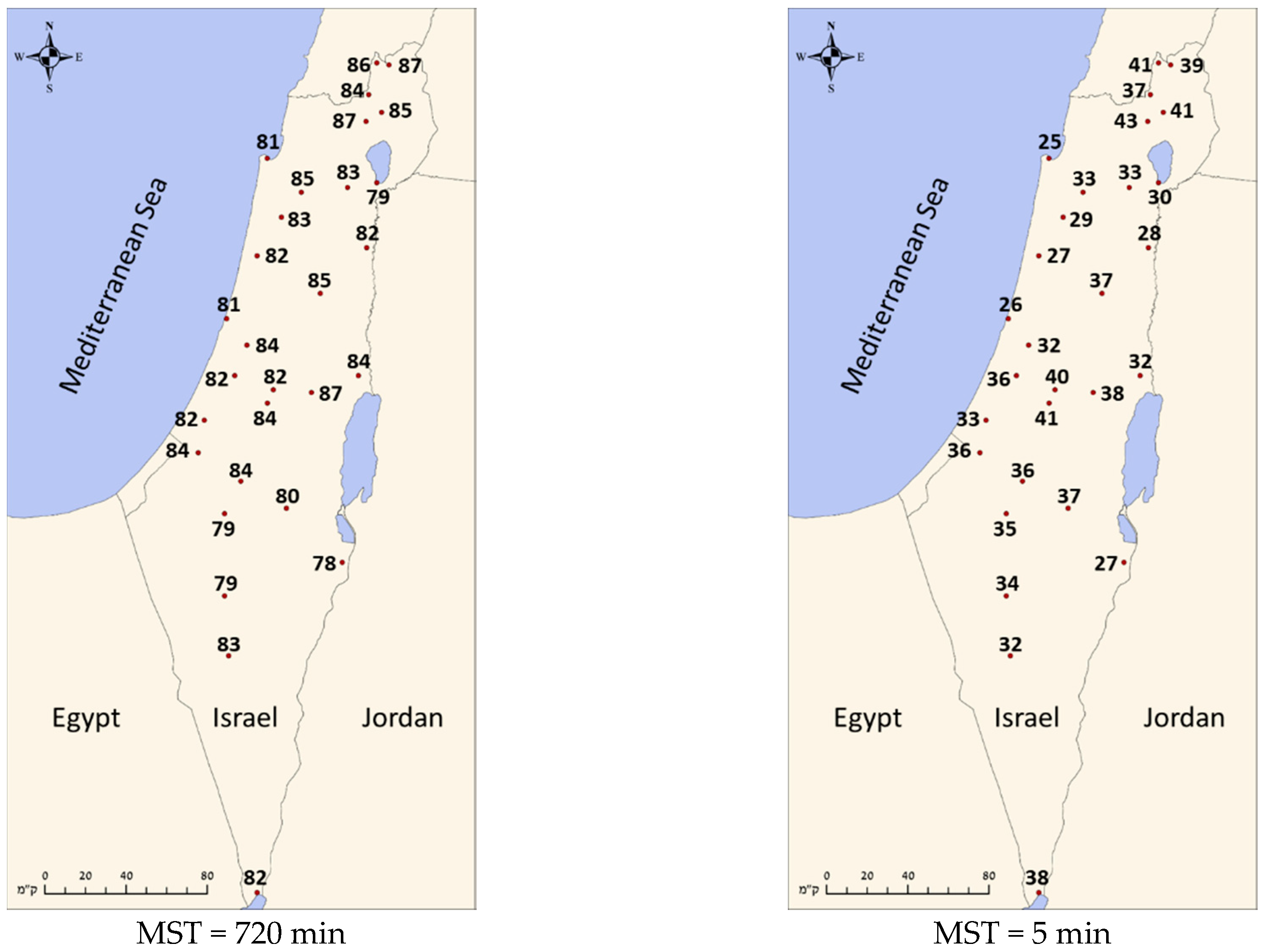
Figure 8, presents the ratio (in percentages) of the Wet Time Duration (WTD) from the Rain Spell Duration for two different Minimum Separation Time (MST), 720 min (12 h.) and 5 min in Israel. These results are based on a MA Thesis by [24]. It should be made clear that as the MST is shorter, additional “no-rain” sub-periods are extracted from the total duration without any change in the total accumulated rainfall and therefore the intensity of the event increases and approaches the “real” intensity. Figure 8a, shows the percentage of WTD from the RSD for a MST = 720 min. It can be noticed that most values are around 80% regardless of their location and mean annual precipitation which varies from 900 mm in the north of the country to 25 mm in the south. Figure 8b, shows the same for a MST = 5 min. Values varies between 25% and 40%, again with no significant differences between north and south. These values imply that if one wants to evaluate the “real” rainfall intensity, he should multiply the average intensity calculated from daily data by a factor ranging between 2.5 (40%) to 4 (25%).
Rainfall intensity is the main climatic factor (together with other non-climatic variables such as soil type, soil depth, slope, antecedent moisture, vegetation cover, etc.) that determines the rate of percolation and/or development of runoff. This in turn determines the rate and amount of soil erosion. These factors are of prime importance for a series of environmental processes and crucial for agriculture. Therefore, the mean daily rainfall intensity for the same stations and the same period as in Figure 7 are presented in Figure 9. Here each figure represents an averaging of a larger number cases as the average number of rain days varies between 42 in Ceylanpinar (in south-eastern Turkey, near the Syrian border) to 142 in Rize. Despite this major averaging, differences between Figure 9a (showing the lowest RSI) and Figure 9b (highest RSI), are enormous. No instantaneous rainfall measurements exist for the stations presented in Figure 7 and Figure 9. Therefore if one wishes to estimate the “real” rainfall intensity in Turkey, the presented averaged daily intensities in Figure 9 should be multiplied at least by a factor of 2.5. This is based on the assumption that most rain events in both countries (Turkey and Israel) originate from the same region and their characteristics (in term of intervals within a rain event) are similar. Doing so, leads to very high instantaneous rainfall intensities which may cause severe floods and soil erosion.
3.1.5. Uncertainty in Intervals
One of the most crucial problems regarding the rainfall regime are intervals between rain-spells or in other words, dry-spells. The Mediterranean Basin is characterized by sunny dry summers, that can last on average from two to six or even seven months in some regions. This is a major advantage for tourism but presents a big challenge for agriculture as the growing season is relatively very short restricted to the so-called “rainy season”. However, this season comprises also of many dry periods which in some cases may last for several weeks with severe consequences.
4. Dryness
Dryness has negative consequences on the environment, economy and societies in many regions around the world. Prolonged dry periods or drought events may affect water supply, causes large damages to the agriculture and the environment, enhance and intensify forest fires [25] and land degradation. A long drought may affect and limit to some extent tourism, as tourism is a high water consumer [26]. Ref. [27], pointed out some of the consequences due to prolonged droughts in a series of Mediterranean tourist resorts in Majorca, southern Spain, Portugal, Crete and so forth. There are large differences between high income countries (mainly European) characterized by high water use efficiencies (typically under 200 l per guest night), whereas, low income countries mainly in North Africa and Asia, showed very high water usage rates (around 900 L per guest night [28]. On the other hand, lack of rainfall may be favourable for many outdoor activities.
There is a very large variability in dryness both in space (from one station to another) and in time (from one year to another and/or along the year). Dryness can be quantified in various ways. One common widely used approach is “dry-spells”. However, ref. [29,30,31,32] and many others, pointed out the advantage of the DDSLR (dry days since last rain) approach upon the dry-spell approach. According to the DDSLR approach each calendar day is attributed a number that represents its distance (in days) since the last rainy day (above any selected daily rainfall threshold-DRT). Each rain day is attributed with a “0” value. Values are accumulated from one year to the next one and then, all values are sorted in an ascending order for each calendar day. This procedure enables the presentation of dryness duration on each calendar day in a probabilistic way using the following equation:
where p is the probability, m is the rank of the of the value in an ascending order and n is the number of observations.
A further detailed description of this methodology can be found in [29].
Three different metrics of the dryness are defined; its severity, consistency and temporal uncertainty (TU):
The severity of the dryness measures the length of the longest dry period.
The consistency considers how frequent (percentage of years) is a dry period of a given length.
The temporal uncertainty considers the span of time (in days) when a dry period of a certain duration can be expected.
Detailed information regarding how these metrics are calculated can be found in [32]. It should be made clear that each of these three metrics are calculated independently without high correlation among them.
Furthermore, no real correlation exists between mean annual rainfall and any of these metrics. Dryness can be a real issue in stations with abundant rainfall while much less so in stations with moderate annual rainfall. The example below illustrates this.
Table 1 presents the mean annual rainfall, the severity, consistency and the temporal uncertainty of DDSLR > 30 days and the return period (R.P.) for such events in 22 stations located in Serbia and Montenegro (Figure 10). It can be noticed that there is absolutely no correlation between any of these metrics and mean annual rainfall. Therefore, a detailed study is needed and one cannot speculate about the dryness conditions in a certain location just by looking at the annual rainfall in that location. In three of the driest stations Palić (mean annual rainfall 526 mm), Niš (558 mm) and Vranje (570 mm) located in inland Serbia the R.P. for a DDSLR > 30 is once every 20 years. On the other hand, three among the rainiest stations Ulcinj (1207 mm), Bar (1346 mm) and Herceg Novi (1737 mm) located on the Adriatic coast of Montenegro, present the highest consistency of DDSLR > 30 days with a R.P. of once every 5, 6 or 7 years respectively. In Ulcinj and Bar a DDSLR > 60 days can be expected once every 29 years (not shown). These examples illustrate the great variability of the rainfall regime between Serbia and Montenegro as revealed for example, by [33]. However, such large variability exists almost everywhere around the Mediterranean for example, in Spain [34], in Israel [25] and in Turkey [32].
5. Discussion and Conclusions
The present article describes a series of causes and factors that may enhance uncertainty in various aspects. Several examples from different regions within the Mediterranean Basin were presented, quantified, analysed and discussed. Many other examples exist and there is no room to list or present them all. According to a very recent article by [35], extremity is expected to increase in the period 2041–2070 at least in Israel for which the analysis was made. As climate is not limited by political borders, it will not be a wild guess to assume that similar trends will be observed also in other parts of the Levant and even further beyond. Increasing extremity, means increasing uncertainty.
5.1. Tourism and Agriculture in the Mediterranean Basin
Two main economic activities characterize the Mediterranean Basin; agriculture and tourism. The main touristic attractions in the Mediterranean Basin are outdoor recreational activities.
Even though that the share of agriculture of the total GDP decreased worldwide in the last decades it is still a major activity in the countries bordering the Mediterranean with an average share of 6.7% in 2016 [36]
Over 320 million tourists were hosted in the countries bordering the Mediterranean in 2015 [37] almost one third of the total number of tourists in the world, with an average share of 19% of tourism out of total export in 2015 [36] or 10% of the GDF [38]. This figure is forecasted to increase to 500 million tourists by 2030 [39].
These two activities are affected mainly by physical factors and by a series of administrative and management regulations and political decisions. The physical factors consist mainly physiographic properties, soil characteristics, climate and weather conditions. The role of climate conditions in influencing touristic activities was discussed in several studies (e.g., [40,41,42,43,44]) made attempts to predict future climate conditions favourable or unfavourable for tourism activities based on scenarios of climate change, the former at a global scale, the latter, for Spain. Among the administrative and management regulations we may mention economic agreements, taxation, monetary policy, manpower allocation, water supply and pricing, marketing policies, transportation, hostile actions and so on. Both activities, agriculture and tourism, need a high degree of certainty to allow an optimal planning and managing of the activities for the next years and decades. However, while economic agreements, taxation, monetary policy and so forth, are all regulated and implemented by men, we have no control on the physical factors, namely climate and weather conditions. It is believed that governments act in a rational way in order to minimalize the uncertainties related to management decisions and allow a realistic planning and management of these two major economic activities. However, no such control of the uncertainty related to the physical factors is possible and therefore climatic uncertainties have a crucial impact on the actual management and future planning of both agriculture and tourism, mainly outdoor recreational activities in the Mediterranean Basin. As agriculture in the Mediterranean Basin is highly dependent on irrigation on the one hand and water resources are limited in large parts of the Mediterranean, [45] and more recently, [46] pointed out the societal and environmental conflicts due to water allocation to the various sectors. They also mentioned the large inter-annual variability of the rainfall regime as one of the factors that reduces the ability of a more realistic allocation.
Ref. [43] present a shift in the timing of the optimal tourism climatic index (TCI) and their duration. They claim that in the future, the main summer months of June-August for “sun and sand” tourists may be too hot in southern European countries (Spain, France, Italy and Greece) and the main touristic period may be split into two periods and/or vacations’ destinations may move to northern cooler locations. An increased uncertainty, regarding the timing of peak temperatures and the onset of the rainy season reduces considerably the ability of tourism managers to make reasonable long term planning. This uncertainty establishes similar challenges also for agriculture planning for example, in water allocation. Whereas, to some extent, decision makers can reduce some uncertainties by making some regulations, unexpected political issues may alter their decisions. However, no regulation or control exist regarding uncertainties related to the natural behaviour of the weather or climate. The results presented above are not the most extreme within the Mediterranean Basin and therefore should be regarded as representing average conditions. Furthermore, in many cases, such as for example dryness in Turkey [32] trends towards increasing uncertainties were detected, even if not always statistically significant.
5.2. Main Conclusions
The main conclusions may be summarized as follows:
The Mediterranean Basin is characterized by a large climatic variability either in space and in time.
Accurate quantification of this variability requires dense measurements which in many cases are not enough.
Lack of enough measurements (e.g., rain gauge density), use of inappropriate approaches in handling or analysing data (e.g., assuming continuity for discrete variables), erroneous interpretation of results (e.g., interpretation of averaged dynamical pressure maps), may increase our uncertainty regarding the behaviour of the parameter in question.
While uncertainty may be exhibited in three main aspects; in the magnitude, timing and location of an event, the implications on a wide range of fields, may differ from one field to another.
Temporal rainfall uncertainty can be detected either in long-term trends, inter-annual and/or intra-annual variability.
Examples regarding the timing, duration, intensity and intervals between events from various locations within the Mediterranean Basin, were presented and discussed.
Trends toward more extreme cases and increasing uncertainty were reported.
A combination of the existing large uncertainty, anticipated increasing variability and a rapid population growth, will result in additional demands for water allocation for domestic use and for other activities such as tourism and agriculture. This will increase challenges for a rational planning of a large spectrum of activities in the Mediterranean Basin.
Funding
This research received no external funding.
Conflicts of Interest
The authors declare no conflict of interest.
List of Acronyms
| DDSLR | dry days since last rain |
| DRT | daily rainfall threshold |
| MSD | mid-season date |
| MST | minimum separation time |
| NRS | number of rain-spells |
| RSBD | rainy season beginning date |
| RSD | rain-spell duration |
| RSED | rainy season ending date |
| RSI | rain-spell intensity |
| RSL | rainy season length |
| TCI | tourism climatic index |
| WTD | wet time duration |
References
- UNDESA. World Population Prospects the 2010 Revision; United Nations: New York, NY, USA, 2010; Volume 1, 405p. [Google Scholar]
- Giorgi, F.; Lionello, P. Climate change projections for the Mediterranean region. Glob. Planet. Chang. 2008, 63, 90–104. [Google Scholar] [CrossRef]
- Milano, M.; Ruelland, D.; Fernandez, S.; Dezetter, A.; Fabre, J.; Servat, E.; Fritsch, J.-M.; Ardoin-Bardin, S.; Thivet, G. Current state of Mediterranean water resources and future trends under climatic and anthropogenic changes. Hydrol. Sci. J. 2013, 58, 498–518. [Google Scholar] [CrossRef] [Green Version]
- Willows, R.; Reynard, N.; Meadowcroft, I.; Connell, R. Climate Adaptation: Risk, Uncertainty and Decision-Making, Part 2; UK Climate Impacts Programme: Oxford, UK, 2003; pp. 41–87. [Google Scholar]
- Hawkins, E.; Sutton, R. The potential to narrow uncertainty in regional climate predictions. Am. Meteorol. Soc. 2009, 1095–1107. [Google Scholar] [CrossRef]
- Hallegatte, S.; Shah, A.; Lempert, R.; Brown, C.; Gill, S. Investment Decision Making Under Deep Uncertainty, Application to Climate Change. In Policy Research Working Paper 6193; The World Bank, Sustainable Development Network, Office of the Chief Economist: Washington, DC, USA, 2012; 39p. [Google Scholar]
- Von Storch, H.; Zwiers, F.W. Statistical Analysis in Climate Research; Cambridge University Press: Cambridge, MA, USA, 2002; 484p. [Google Scholar]
- Kay, P.A.; Kutiel, H. Some remarks on climatic maps of precipitation. Clim. Res. 1994, 4, 233–241. [Google Scholar] [CrossRef]
- Kutiel, H.; Kay, P.A. Effects of network design on climatic maps of precipitation. Clim. Res. 1996, 7, 1–10. [Google Scholar] [CrossRef] [Green Version]
- Mishra, A.K. Effect of rain gauge density over the accuracy of rainfall: A case study over Bangalore, India. SpringerPlus 2013, 2, 311. [Google Scholar] [CrossRef] [PubMed]
- Xu, H.; Xu, C.U.; Chen, H.; Zhang, Z.; Li, L. Assessing the influence of rain gauge density and distribution on hydrological model performance in a humid region of China. J. Hydrol. 2013, 505, 1–12. [Google Scholar] [CrossRef]
- Lopez, M.G.; Wennerström, H.; Nordén, L.Å.; Seibert, J. Location and density of rain gauges for the estimation of spatial varying precipitation. Swed. Soc. Anthropol. Geogr. 2015, 167–179. [Google Scholar] [CrossRef]
- Paz, S.; Kutiel, H. Rainfall regime uncertainty (RRU) in an eastern Mediterranean region—A methodological approach. Israel J. Earth Sci. 2003, 52, 47–63. [Google Scholar] [CrossRef]
- Aviad, Y.; Kutiel, H.; Lavee, H. Analysis of beginning, end and length of the rainy season along a Mediterranean–arid climate transect for geomorphic purposes. J. Arid Environ. 2004, 59, 189–204. [Google Scholar] [CrossRef]
- Reiser, H.; Kutiel, H. Rainfall uncertainty in the Mediterranean: Definition of the Daily Rainfall Threshold (DRT) and the Rainy Season Length (RSL). Theor. Appl. Climatol. 2009, 97, 151–162. [Google Scholar] [CrossRef]
- Kutiel, H.; Trigo, R.M. The rainfall regime in Lisbon in the last 150 years. Theor. Appl. Climatol. 2014, 118, 387–403. [Google Scholar] [CrossRef]
- Hernández, A.; Kutiel, H.; Trigo, R.M.; Valente, M.A.; Cropper, T.; Espírito Santo, F. New Azores archipelago daily precipitation dataset and its links with large-scale modes of climate variability. Int. J. Climatol. 2016. [Google Scholar] [CrossRef]
- Baldi, M.; Pasqui, M.; Cesarone, F.; De Chiara, G. Heat waves in the Mediterranean region: Analysis and model result. In Proceedings of the 16th Conference on Climate Variability and Change, San Diego, CA, USA, 9 January 2005; pp. 9–13. [Google Scholar]
- Encyclopedia Britannica. Available online: https://www.britannica.com/event/European-heat-wave-of-2003 (accessed on 21 December 2018).
- Russo, A.; Gouveia, C.M.; Ramos, A.M.; Páscoa, P.; Trigo, R.M. The association between preceding drought occurrence and heat waves in the Mediterranean. In Proceedings of the 19th EGU General Assembly (EGU2017), Vienna, Austria, 23–28 April 2017; p. 17700. [Google Scholar]
- Dunkerley, D. Rain event properties in nature and in rainfall simulation experiments: A comparative review with recommendations for increasingly systematic study and reporting. Hydrol. Process. 2008, 22, 4415–4435. [Google Scholar] [CrossRef]
- Dunkerley, D.L. How do the rain rates of sub-event intervals such as the maximum 5- and 15-min rates (I5 or I30) relate to the properties of the enclosing rainfall event? Hydrol. Process. 2010, 24, 2425–2439. [Google Scholar]
- Dunkerley, D. Intra-event intermittency of rainfall: An analysis of the metrics of rain and no-rain periods. Hydrol. Process. 2015, 29, 3294–3305. [Google Scholar] [CrossRef]
- Weisskopf, Y. Analysis of Intra-Storm Rain Episodes in Israel. Master’s Thesis, Department of Geography and Environmental Studies, University of Haifa, Haifa, Israel, 2014. (In Hebrew with English Summary). [Google Scholar]
- Wittenberg, L.; Kutiel, H. Dryness in Mediterranean type climate—Implication on wildfires burnt area—A case study from Mt. Carmel, Israel. Int. J. Wildland Fire 2016, 25, 579–591. [Google Scholar] [CrossRef]
- Gössling, S.; Peeters, P.; Hall, C.M.; Ceron, J.-P.; Dubois, G.; Lehmann, L.V.; Scott, D. Tourism and water use: Supply, demand and security. An international review. Tour. Manag. 2012, 33, 1–15. [Google Scholar] [CrossRef]
- Perry, A.H. Impacts of Climate Change on Tourism in the Mediterranean: Adaptive Responses; FEEM Working Paper No. 35; Fondazione Eni Enrico Mattei: Milan, Italy, 2000; 11p. [Google Scholar]
- Becken, S. Water equity—Contrasting tourism water use with that of the local community. Water Resour. Ind. 2014, 7–8, 9–22. [Google Scholar] [CrossRef]
- Aviad, Y.; Kutiel, H.; Lavee, H. Variation of Dry Days Since Last Rain (DDSLR) as a measure of dryness along a Mediterranean—Arid transect. J. Arid Environ. 2009, 73, 658–665. [Google Scholar] [CrossRef]
- Reiser, H.; Kutiel, H. Rainfall uncertainty in the Mediterranean: Dryness distribution. Theor. Appl. Climatol. 2010, 100, 123–135. [Google Scholar] [CrossRef]
- Lana, X.; Burgueno, A.; Martinez, M.D.; Serra, C. Some characteristics of a daily rainfall deficit regime based on the dry day since last rain index (DDSLR). Theor. Appl. Climatol. 2012, 109, 153–174. [Google Scholar] [CrossRef]
- Kutiel, H.; Türkeş, M. Spatial and temporal variability of dryness characteristics in Turkey. Int. J. Climatol. 2017. [Google Scholar] [CrossRef]
- Kutiel, H.; Luković, J.; Burić, D. Spatial and temporal variability of rain-spells characteristics in Serbia and Montenegro. Int. J. Climatol. 2015, 35, 1611–1624. [Google Scholar] [CrossRef]
- Ruiz-Sinoga, J.D.; Garcia-Marin, R.; Gabarron-Galeotea, M.A.; Martinez-Murillo, J.F. Analysis of dry periods along a pluviometric gradient in Mediterranean southern Spain. Int. J. Climatol. 2012, 32, 1558–1571. [Google Scholar] [CrossRef]
- Hochman, A.; Mercogliano, P.; Alpert, P.; Saaroni, H.; Bucchignani, E. High-resolution projection of climate change and extremity over Israel using COSMO-CLM. Int. J. Climatol. 2018. [Google Scholar] [CrossRef]
- World Bank. Available online: https://data.worldbank.org/indicator/NV.AGR.TOTL.ZS?locations=1W (accessed on 21 December 2018).
- MGI (Mediterranean Growth Initiative). Tourism in the Mediterranean. 2017. Available online: https://www.mgi.online/content/2017/8/4/tourism-in-the-mediterranean (accessed on 21 December 2018).
- Lanquar, R. Tourism in the Mediterranean: Scenarios up to 2030; MEDPRO Report No. 1/July 2011 (Updated May 2013); CEPS: Brussels, Belgium, 2013; 40p. [Google Scholar]
- UNWTO. UNWTO Annual Report 2012; World Tourism Organization: Madrid, Spain, 2012; 82p. [Google Scholar]
- Gómez Martín, B. Weather, climate and tourism a geographical perspective. Ann. Tour. Res. 2005, 32, 571–591. [Google Scholar] [CrossRef]
- Goh, C. Exploring of climate on tourism demand. Ann. Tour. Res. 2012, 39, 1859–1883. [Google Scholar] [CrossRef]
- Rosselló-Nadal, J. How to evaluate the effects of climate change on tourism. Tour. Manag. 2014, 42, 334–340. [Google Scholar] [CrossRef]
- Amelung, B.; Nicholls, S.; Viner, D. Implications of Global Climate Change for Tourism Flows and Seasonality. J. Travel Res. 2007, 45, 285–296. [Google Scholar] [CrossRef]
- Hein, L.; Metzger, M.J.; Moreno, A. Potential impacts of climate change on tourism; a case study for Spain. Curr. Opin. Environ. Sustain. 2009, 1, 170–178. [Google Scholar] [CrossRef]
- Iglesias, A.; Mougou, R.; Moneo, M.; Quiroga, S. Towards adaptation of agriculture to climate change in the Mediterranean. Reg. Environ. Chang. 2011, 11, S159–S166. [Google Scholar] [CrossRef]
- Cramer, W.; Guiot, J.; Fader, M.; Garrabou, J.; Gattuso, J.P.; Iglesias, A.; Lange, M.A.; Lionello, P.; Llasat, M.C.; Paz, S.; et al. Climate change and interconnected risks to sustainable development in the Mediterranean. Nat. Clim. Chang. 2018, 8, 972–980. [Google Scholar] [CrossRef]
Figure 1.
Schematic representation of various parameters affecting the uncertainty of a climatic variable.
Figure 1.
Schematic representation of various parameters affecting the uncertainty of a climatic variable.

Figure 2.
Mean daily air temperature [K] maps at the 1000 hPa level based on NCEP reanalysis daily averages. Average map for the period 1 December 2017–28 February 2018 and some selected daily maps.
Figure 2.
Mean daily air temperature [K] maps at the 1000 hPa level based on NCEP reanalysis daily averages. Average map for the period 1 December 2017–28 February 2018 and some selected daily maps.


Figure 3.
Same as Figure 2 but for geopotential heights [gpm].
Figure 3.
Same as Figure 2 but for geopotential heights [gpm].


Figure 4.
A schematic representation of a depression over some parts of Italy. In both cases the atmospheric pressure over Rome is identical (1005 hPa) however, prevailing flow are from different directions causing completely different weather conditions.
Figure 4.
A schematic representation of a depression over some parts of Italy. In both cases the atmospheric pressure over Rome is identical (1005 hPa) however, prevailing flow are from different directions causing completely different weather conditions.

Figure 5.
Schematic representation of various types and components of climatic uncertainty. The present article deals with those components shown in bold.
Figure 5.
Schematic representation of various types and components of climatic uncertainty. The present article deals with those components shown in bold.

Figure 6.
Range of dates when 50% of the annual rainfall was accumulated and range of percentage accumulated on the median MSD (26 June) in Belgrade, Serbia.
Figure 6.
Range of dates when 50% of the annual rainfall was accumulated and range of percentage accumulated on the median MSD (26 June) in Belgrade, Serbia.

Figure 7.
Mean annual rain-spell duration (RSD) in Turkey (1970–2011).


Figure 8.
Percentage of Wet Time Duration (WTD) from Rain Spell Duration (RSD) for two selected Minimum Separation Time (MST).
Figure 8.
Percentage of Wet Time Duration (WTD) from Rain Spell Duration (RSD) for two selected Minimum Separation Time (MST).

Figure 9.
Mean annual rain-spell intensity (RSI) in Turkey (1970–2011).

Figure 10.
Location map of the stations in Serbia and Montenegro.


Table 1.
Three metrics of the DDSLR in selected stations in Serbia and Montenegro. Stations are arranged in an ascending order of their mean annual rainfall. The severity represents the longest DDSLR, the consistency, the percentage of years with DDSLR longer than 30 days and the temporal uncertainty, the span of days along the year when such an event may be expected. The return period (R.P.) of a DDSLR longer than 30 days is also presented.
| Station | Mean Annual Rainfall [mm] | Severity [days] | Consistency [% of years] | R.P. [years] | Temporal Uncertainty [days] |
|---|---|---|---|---|---|
| Palić | 526.2 | 55 | 5.1 | 20 | 173 |
| Kikinda | 543.9 | 60 | 8.9 | 11 | 159 |
| Niš | 558.1 | 67 | 5.1 | 20 | 205 |
| Vranje | 569.5 | 67 | 5.1 | 20 | 166 |
| Zrenjanin | 576.6 | 60 | 10.7 | 9 | 153 |
| Novi Sad | 583.2 | 72 | 10.2 | 10 | 190 |
| Zajecar | 594.0 | 67 | 7.1 | 14 | 157 |
| Novi Pazar | 605.7 | 60 | 5.4 | 19 | 153 |
| Sremska Mitrovica | 615.1 | 51 | 5.1 | 20 | 104 |
| Kragujevac | 618.8 | 53 | 5.1 | 20 | 123 |
| Negotin | 641.1 | 68 | 8.9 | 11 | 209 |
| Veliko Gradiste | 647.9 | 53 | 6.8 | 15 | 132 |
| Belgrade | 679.8 | 48 | 5.1 | 20 | 117 |
| Kraljevo | 739.4 | 44 | 3.4 | 29 | 61 |
| Pljevlja | 785.9 | 72 | 3.4 | 29 | 99 |
| Loznica | 832.1 | 51 | 3.6 | 28 | 50 |
| Ulcinj | 1207.2 | 80 | 20.3 | 5 | 204 |
| Bar | 1345.8 | 72 | 16.9 | 6 | 186 |
| Herceg Novi | 1737.4 | 53 | 13.6 | 7 | 157 |
| Niksic | 1849.6 | 53 | 8.5 | 12 | 148 |
| Kolašin | 2077.1 | 48 | 5.1 | 20 | 74 |
| Crkvice | 4396.9 | 52 | 5.4 | 19 | 145 |
© 2019 by the author. Licensee MDPI, Basel, Switzerland. This article is an open access article distributed under the terms and conditions of the Creative Commons Attribution (CC BY) license (http://creativecommons.org/licenses/by/4.0/).
Share and Cite
MDPI and ACS Style
Kutiel, H. Climatic Uncertainty in the Mediterranean Basin and Its Possible Relevance to Important Economic Sectors. Atmosphere 2019, 10, 10. https://doi.org/10.3390/atmos10010010
AMA Style
Kutiel H. Climatic Uncertainty in the Mediterranean Basin and Its Possible Relevance to Important Economic Sectors. Atmosphere. 2019; 10(1):10. https://doi.org/10.3390/atmos10010010
Chicago/Turabian StyleKutiel, Haim. 2019. "Climatic Uncertainty in the Mediterranean Basin and Its Possible Relevance to Important Economic Sectors" Atmosphere 10, no. 1: 10. https://doi.org/10.3390/atmos10010010
Note that from the first issue of 2016, this journal uses article numbers instead of page numbers. See further details here.