Horizontal Vortex Tubes near a Simulated Tornado: Three-Dimensional Structure and Kinematics
by
 , , ,
, , ,
Maurício I. Oliveira
1 ,
,
Ming Xue
1,*,
Brett J. Roberts
2,3,4,
Louis J. Wicker
2 and
Nusrat Yussouf
2,4 1
Center for Analysis and Prediction of Storms and School of Meteorology, University of Oklahoma, Norman, OK 73072, USA
2
National Severe Storms Laboratory, NOAA, Norman, OK 73072, USA
3
Storm Prediction Center, NWS/NOAA, Norman, OK 73072, USA
4
Cooperative Institute for Mesoscale Meteorological Studies, University of Oklahoma, Norman, OK 73072, USA
*
Author to whom correspondence should be addressed.
Atmosphere 2019, 10(11), 716; https://doi.org/10.3390/atmos10110716
Submission received: 1 October 2019
/
Revised: 12 November 2019
/
Accepted: 13 November 2019
/
Published: 16 November 2019
(This article belongs to the Special Issue Simulation and Visualization of Severe Weather)
Abstract
:Supercell thunderstorms can produce a wide spectrum of vortical structures, ranging from midlevel mesocyclones to small-scale suction vortices within tornadoes. A less documented class of vortices are horizontally-oriented vortex tubes near and/or wrapping about tornadoes, that are observed either visually or in high-resolution Doppler radar data. In this study, an idealized numerical simulation of a tornadic supercell at 100 m grid spacing is used to analyze the three-dimensional (3D) structure and kinematics of horizontal vortices (HVs) that interact with a simulated tornado. Visualizations based on direct volume rendering aided by visual observations of HVs in a real tornado reveal the existence of a complex distribution of 3D vortex tubes surrounding the tornadic flow throughout the simulation. A distinct class of HVs originates in two key regions at the surface: around the base of the tornado and in the rear-flank downdraft (RFD) outflow and are believed to have been generated via surface friction in regions of strong horizontal near-surface wind. HVs around the tornado are produced in the tornado outer circulation and rise abruptly in its periphery, assuming a variety of complex shapes, while HVs to the south-southeast of the tornado, within the RFD outflow, ascend gradually in the updraft.
1. Introduction
Supercell thunderstorms produce a wide spectrum of vortical structures with length scales ranging from the large, midlevel mesocyclone (5–10 km in diameter; [1,2]) down to vortices on the order of only a few meters, such as suction vortices [3,4,5]. One such manifestation of strong vorticity in supercells occurs in the form of three-dimensional (3D), elongated vortex tubes that are typically observed near tornadoes or in the periphery of their parent low-level mesocyclones [6,7,8]. They can occasionally be visually observed as condensation tubes or severely slanted funnels, given high-enough relative humidity and/or intense-enough cyclostrophic pressure drop inside them [9,10]. These vortex tubes are anecdotally referred to as “horizontal vortices” since, in contrast to tornadoes that are defined as vertical vortices, the axis of rotation of these vortex tubes is oriented primarily parallel to the ground.
Given the small scale and transient nature of horizontal vortices (hereafter referred to as HVs), they are hard to observe in Doppler radar data or to resolve in high-resolution numerical simulations; most evidence for their existence relies on videos or photographs [7,8,9]. Among the few existing observations, Wurman and Kosiba [5] provide evidence for large HVs south-southeast of two large tornadoes sampled by the Doppler-on-Wheels (DOW) mobile radar. In both cases, the HVs are located outside of the tornadic circulation but their sense of rotation (inferred from radial velocity plan-position indicators at two levels; see their Figure 14) is different; in one case the inferred horizontal vorticity vector points to the southwest while in the other it points to the north-northeast. This suggests different mechanisms may control HV formation. Houser et al. [9] provided an analysis of an HV interacting with the violent Piedmont-El Reno tornado on 24 May 2011 based on Rapid-scan X-Polarimetric Doppler (RaXPol) data and videographic observations. The HV, which is collocated with a weak-reflectivity band in reflectivity data, has a horizontal vorticity vector orientation similar to the Canton tornado case from Wurman and Kosiba [5], which pointed to the northeast and originated in a rear-flank downdraft (RFD) internal momentum surge to the south-southeast of the tornado, close to the surface. The HV wraps around the intensifying tornado, ascending in its circulation. The authors suggest possible mechanisms for the formation of the HV consistent with the observed horizontal vorticity vector orientation, which include: (i) baroclinic production along a warm RFD surge behind the primary RFD gust front, (ii) frictional torques in outflow air also behind the primary RFD gust front and (iii) reorientation of vertical vorticity associated with the tornado into a horizontal axis. Regardless of the mechanism, horizontal stretching of the vortex tube into the intensifying tornado is responsible for strengthening the HV to the point that cyclostrophic pressure drop in its core caused condensation to form.
Orf et al. [10], using a numerical simulation employing 30-m isotropic grid spacing to investigate the 24 May 2011 El Reno supercell and tornado, were the first to describe simulated HVs similar to visual observations. In the simulation, vortices ascend as funnel clouds on the periphery of the simulated tornado, in a similar manner to that described in Houser et al. [9].
As discussed by Houser et al. [9], surface friction is a plausible mechanism that can produce strong near-surface horizontal vorticity in the RFD outflow. This mechanism was shown earlier by Schenkman et al. [11] to have a significant impact on the vorticity budget of a developing tornado in a real case simulation of the 8 May 2003 Oklahoma City (OKC) tornadic storm [12]. In that study, surface friction acts on outflow and inflow parcels to produce strong near-surface horizontal vorticity that is abruptly tilted and stretched to produce pre-tornadic vertical vorticity centers that eventually coalesce into a tornado. This mechanism was explored in detail by Roberts et al. [13] and Roberts and Xue [14] in an idealized, single-sounding simulation of the 3 May 1999 Bridge Creek-Moore tornado. In summary, the authors show that surface friction acting on storm-induced flow produces near-surface crosswise horizontal vorticity that can be exchanged into streamwise vorticity as the flow bends cyclonically when converging toward a developing tornado (i.e., the river bend effect, e.g., Davies-Jones et al. [15]). The vorticity-rich parcels can then be tilted abruptly and stretched to produce strong near-surface vertical vorticity.
In order to better understand the behavior of HVs near strong tornadoes, in this study, data from a 100-m horizontal grid spacing, single-sounding simulation of a tornadic supercell are used to investigate the kinematics and dynamics of HVs near a simulated strong tornado. More specifically, our main objective is to provide a description of the 3D structure, types and evolution of HVs using direct volume rendering (DVR), a visualization technique used to generate high-quality displays of 3D numerical data offered by the Visualization and Analysis Platform for Ocean, Atmosphere, and Solar Researchers (VAPOR; [16,17]) software. The analysis is then validated by comparing the volume rendered vortical flows with visual observations of HVs in a real violent tornado. Finally, the kinematics of the near-ground flow in which HVs originate is briefly evaluated in order to infer potential formation mechanisms. More quantitative analyses of the dynamics within the simulation, including vorticity and circulation budget analyses following parcel trajectories and evolving material circuits, are deferred to future studies.
The reminder of the paper is organized as follows: Section 2 presents the numerical setup and methodology used to obtain the tornado simulation. Section 3 presents an overview of the simulated storm and associated tornadoes. Section 4 describes the structure and kinematics of HVs surrounding a simulated tornado using DVR of vorticity magnitude as compared to visual observations of real HVs, as well as traditional two-dimensional analyses of the vorticity field. Section 5 provides a discussion and summarizes the conclusions.
2. Numerical Experiments
The Advanced Regional Prediction System (ARPS; [18,19,20]) is used to perform the simulation presented in this study. The model domain is 84 km × 84 km in the horizontal, and 16 km in the vertical, with a Rayleigh damping layer applied above 12 km above ground level (AGL). The bottom boundary is flat. The horizontal grid spacing is 100 m and the minimum vertical grid spacing is 2 m at the surface, which stretches to 200 m above 10 km AGL, comprising 83 levels in the vertical.
The minimum vertical grid spacing of 2 m places the lowest scalar grid level at 1 m AGL. The reason for using such a small vertical grid spacing near the ground is twofold: (i) to provide increased vertical resolution very close to the surface and (ii) to place the first scalar model level closer to the surface than what is typically used in convective storm simulation studies (e.g., z ≥ 10 m AGL). Placing the lowest scalar level very close to the model surface is an attempt to increase the sample size of parcel trajectories that do not fall below the lowest scalar level, thus, avoiding the need to rely on extrapolated kinematic quantities [21]. Tornado and HV vorticity budgets along Lagrangian trajectories in this simulation will be examined in a future study, as indicated earlier. The drawback of using very small near-surface grid spacing is that the time step used in the explicit vertical advection scheme must also be very small; otherwise, the linear stability condition can be easily violated, especially when tornadoes are present. Therefore, a large (small) time step of 0.075 s (0.05 s) is used.
Lin et al. [22] ice microphysics is used with the rain intercept parameter N0r set to 2 × 10⁻⁶ m−4, rather than the default value of 8 × 10⁻⁶ m−4. The reduced value can produce more realistic cold pools and sustained tornadic vortices [13,14,23,24]. Fourth-order advection is used in the horizontal and vertical. Subgrid-scale turbulence is parameterized with a 1.5-order turbulent kinetic energy (TKE)-based scheme [25] while fourth-order horizontal and vertical computational mixing coefficients are set to 30 × 10−4 m4 s−1 and 15 × 10−4 m4 s−1, respectively.
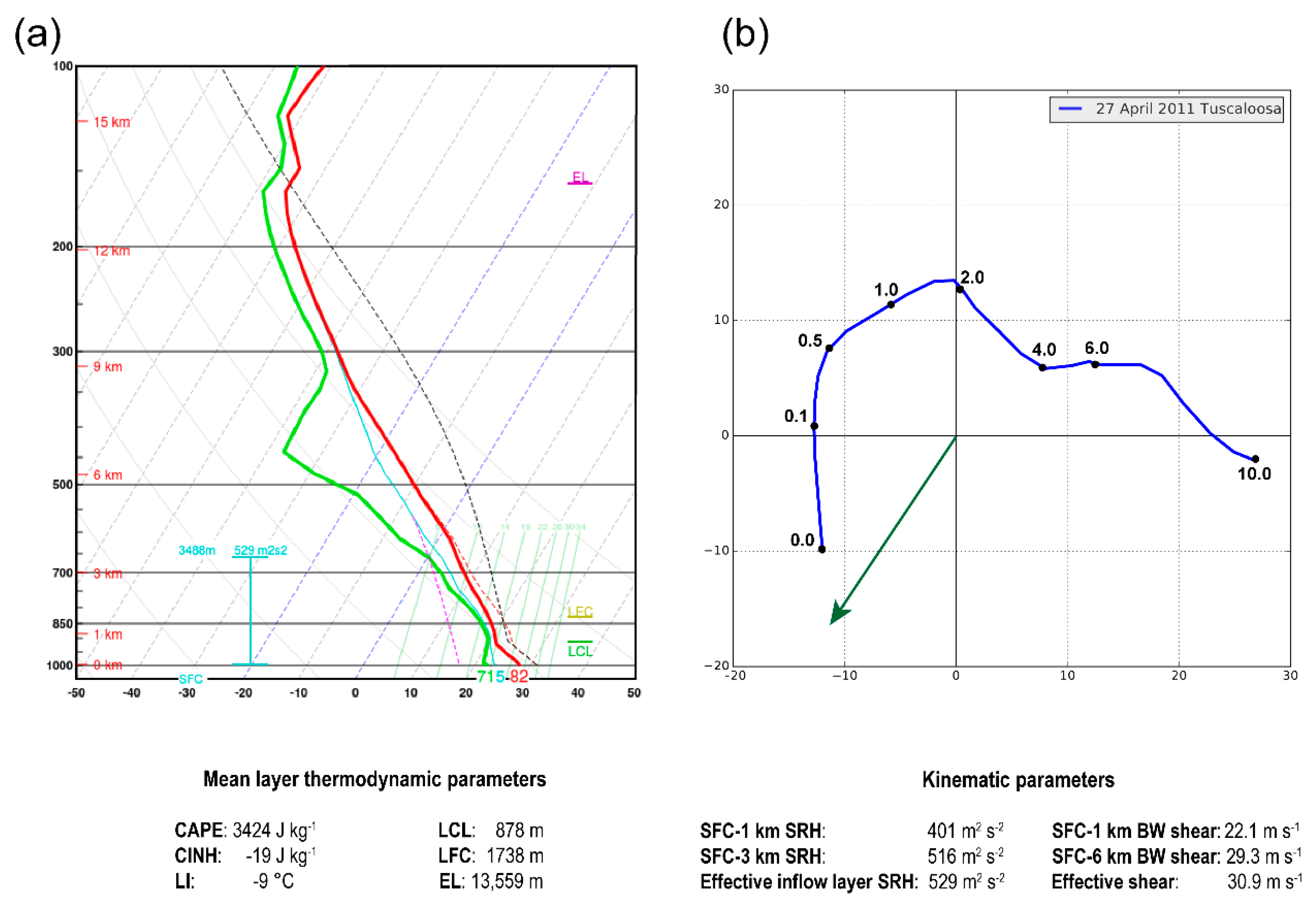
The model supercell storm is triggered by a thermal bubble within a horizontally homogeneous environment defined by a single sounding. The sounding is obtained from a full-physics 3 km grid spacing Weather Research and Forecasting (WRF) model simulation nested within a 15 km grid covering the contiguous United States for the 27 April 2011 devastating tornado outbreak in Mississippi-Alabama [26]. Conventional and radar observations were assimilated on the 15 and 3 km grids, respectively, using ensemble Kalman filter. The model sounding is extracted approximately 40 km southeast of the predicted storm corresponding to the Tuscaloosa-Birmingham tornadic supercell [7,27] at the 2100 Universal Time Coordinated (UTC) analysis time (Figure 1). The analysis time is 1 h before the observed and predicted storms struck Tuscaloosa (at around 2200 UTC). The thermodynamic profile is obtained from a grid point over the city of Tuscaloosa (32.9° N, 85.6° W) and the wind profile is averaged over a 0.2° latitude-longitude box centered on that grid point. A comparison of the surface air and dew-point temperatures at the Tuscaloosa airport (28.0 °C and 21.0 °C, respectively) with the WRF profile (27.8 °C and 21.9 °C, respectively) revealed a good agreement between the observations and WRF analysis. The location and time of the model-extracted sounding match the spatial and temporal ranges for proximity sounding suggested by Potvin [28] and minimize contamination from the predicted storm. A constant wind speed (u = 11 m s−1, v = 17 m s−1) is subtracted from the sounding to keep the simulated supercell quasi-stationary during its tornadic phase. A similar procedure of extracting a sounding from a three-dimensional real-data simulation was taken by, e.g., Dawson et al. [24], as observed soundings at appropriate time and location were not available.
Early, coarse resolution experiments (not shown) had spurious convection forming in the inflow of the developing supercell that eventually contaminated the storm. To avoid this problem, a small temperature increment was added to the sounding in the 720–2900 m layer, with a maximum 1.8 K added to the top of atmospheric boundary layer AGL. This increment rapidly decreases following a fourth-degree polynomial function such that at the bottom (top) of the modified layer, the perturbation is 0.2 K (0.5 K). The depth of the layer and the magnitude of the temperature increment were chosen by trial and error and were found to be the best option to eliminate spurious inflow convection while sustaining a vigorous tornadic supercell storm in the simulation. This procedure reflects the often-present top-of-boundary-layer inversion, and its direct effect was to reduce the mixed-layer Convective Available Potential Energy (MLCAPE) from 3442 J kg−1 to 3424 J kg−1 and increase the magnitude of Convective Inhibition (MLCINH) from 0 J kg−1 to 19 J kg−1, respectively. Convection is initiated with an ellipsoidal thermal bubble perturbation centered at y = 66 km and x = 16 km with a horizontal (vertical) radius of 10 km (1.5 km). The maximum potential temperature perturbation at the center of the bubble is 6 K. This larger than typically used bubble amplitude is needed to develop a sustained supercell because of the larger inhibition added to the sounding as well as the large low-level wind shear in the environment.
The bottom boundary condition is semi slip with a constant drag coefficient Cd of 2.8 × 10⁻² applied to the surface horizontal momentum stress terms in the subgrid-scale turbulence parameterization scheme [13,14]. The value of Cd employed corresponds to an equivalent roughness length of 9.16 cm. The straightforward inclusion of surface drag in idealized convective storm simulations has the undesired effect of constantly slowing down the initial near-ground wind profile [30], destroying the base-state kinematic environment. In order to avoid this problem, the large-scale balance (LSB) technique discussed in Dawson et al. [31] is used. The fundamental idea in this technique is to assume that the initial horizontal wind profile is in a three-way balance among the horizontal-pressure gradient, Coriolis and frictional forces. Since the latter two forces are known from the initial wind profile, a pseudo-pressure gradient force is computed from the model time tendency of momentum equations at the first time step (i.e., before any modification caused by surface drag) for each model column. The pseudo-pressure gradient force (calculated for each grid point) is then added to the right-hand side of the horizontal momentum equations at all times at every grid point. The result is that the initial base-state wind profile remains virtually unchanged throughout the model integration.
Model integration is carried out using mode splitting, with the leapfrog (forward-backward) scheme for the slow (fast acoustic) modes. The model is integrated until 14,270.175 s using the 0.075 s large step. However, at this time, a tornado with strong near-surface updrafts is underway, and the vertical advection stability limit is violated since the first model layer is very shallow. From this time on, the simulation is restarted and run until 4 h 20 min using a large time step of 0.025 s while the small time step size is kept at 0.05 s. This is possible because vertical acoustic wave propagation is treated implicitly in the ARPS so that the small time step size is limited by horizontal grid spacing only. The large time step size is on the other hand limited by the very small vertical grid spacing in the case of large vertical velocity. The acoustic wave models are integrated using forward-backward integration schemes with time step size ∆τ, starting from the past time level t – ∆t and ending the future time level t + ∆t, in n number of “small” time steps. When n = 1, ∆τ = 2∆t, hence the ‘small’ time step size is twice as large as the ‘large’ time step size [32,33].
3. Simulated Storm Overview
The simulated storm is fully developed into a supercell (e.g., with a hook-like appendage in the rainwater field and well-defined forward- and RFD gust fronts; Figure 2a) after 1 h of model integration as it gradually moves northwestward within the domain. This northwestward motion persists (but slows down) during the first 3 h of simulation. During this period, the storm develops only mesocyclone-scale vertical vorticity of O(10−2 s−1) at low levels (Figure 2a–c), with multiple low-level mesocyclone cycles taking place. However, tornado-intensity vortices do not develop until later in the simulation, a behavior that differs from the observed supercells in the 27 April 2011 tornado outbreak which were prolific tornado producers during a significant fraction of their life span. Several reasons may explain the differences between the simulated and observed storms as well the delayed tornado development in the simulation, which include: (i) inherent errors in the initial sounding extracted from the WRF analysis, (ii) the idealized, horizontally homogeneous design of the simulation that excludes heterogeneous environmental conditions encountered by the observed storm (e.g., complex terrain, cell mergers; [7,27]) and (iii) thermodynamic modifications applied to the initial sounding to prevent spurious convection. It should be pointed out, however, that early coarse grid spacing simulations (not shown) displayed a similar tendency for the storm to delay the production of strong surface vertical vortices in the first 2–3 h of integration, suggesting the delayed production of strong vortices may also be linked to the larger vertical shear present in the base-state wind profile [34].
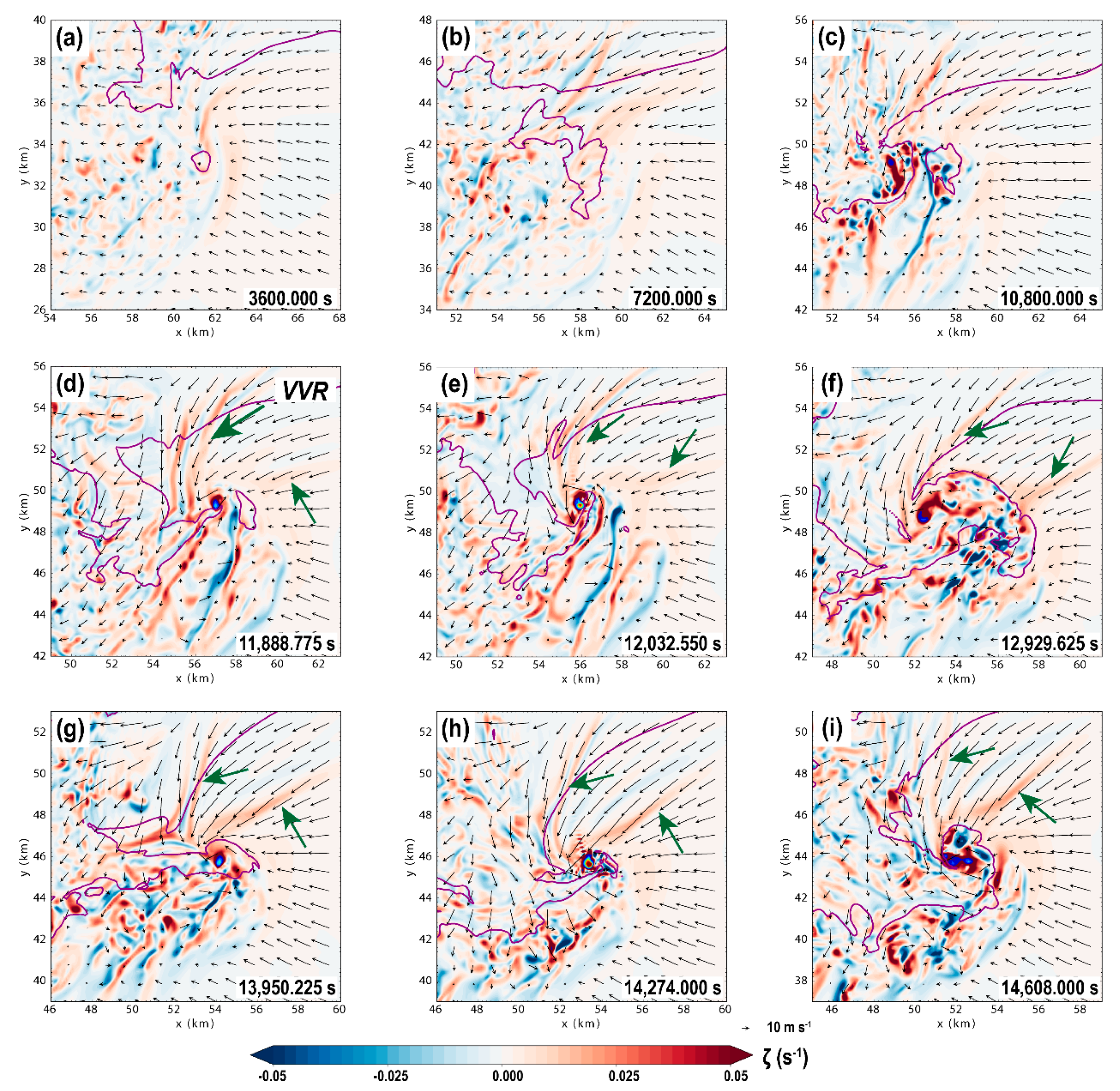
After 3 h 16 min, significant structural changes occur in the supercell. Rapid strengthening of the low-level updraft at the tip of the hook (not shown) occurs coincidently with a sharpening (i.e., increase in confluence) of a left-flank convergence boundary (LFCB, as in Beck and Weiss [35]; compare Figure 2c,d). The increase in the degree of organization of the LFCB results in the formation of meridionally-oriented “vertical vorticity rivers” [35,36], which first appear at the base of downdrafts northwest of the low-level circulation (Figure 2d). These features, along with enhanced vertical vorticity in an RFD internal boundary, are thought to be the primary storm-scale sources of vertical vorticity to the developing low-level rotation in other simulations in the literature [35,36,37,38]. At 11,888.775 s, the first tornado forms at the tip of the hook as seen in the vertical vorticity field (Figure 2d, Figure 3a, and Figure 4a). In this study, a tornado is defined as a persistent, concentrated vortex with surface vertical vorticity exceeding 0.1 s−1 and wind speed greater than 29 m s−1, i.e., the minimum wind threshold of an Enhanced Fujita (EF) 0 tornado.
As the tornado matures, it briefly attains a maximum EF3 intensity at 12,032.550 s (Figure 2e, Figure 3b, and Figure 4b), with peak ground-level wind speeds of 62.2 m s−1 at 10 m AGL and surface core width (roughly estimated based on the highly-asymmetric radius of maximum wind at 1 m AGL) of about 200 m. After this short period of intensification, however, the tornado maintains only EF1 wind speeds during most of its life cycle. Throughout its life cycle, the tornado exhibits significant northeastward tilt with height [39] and is stronger near the ground during the tornadogenesis and maintenance phases (Figure 3a,b). In fact, nearly all the violent tornadoes on the 27 April 2011 tornado outbreak displayed pronounced northeastward tilt with height in addition to the almost ubiquitous presence of HVs [7]. The condensation funnel of this first tornado never touches the ground, a result of the insufficient cyclostrophic pressure drop within the tornado vortex.
In addition to the abovementioned LFCB vorticity river, less prominent rivers exist northeast of the tornado (Figure 2e), possibly associated with forward-flank convergence boundaries (FFDBs; [35]). The FFCBs merges with the LFCB just north-northwest of the tornado and may contribute to the vertical vorticity budget of the tornado (a topic that will be addressed in a future study).
After approximately 17 min on the ground, the first tornado becomes completely occluded and wrapped in rain, resulting in broadening of the hook as the dissipating tornado moves rearward (southwestward) relative to the parent supercell [40,41,42] (Figure 2f and Figure 4c). The near-ground vortex becomes completely detached from its upper portion and gradually decays (Figure 3c). The remnant vortex persists as a shrinking area of vertical vorticity embedded in precipitation that eventually mixes out within the turbulent downdraft outflow in the rear part of the storm. Despite that, the hook persists as a large low-level circulation, with an anticyclonic flare to its southeast (e.g., [43,44]) (Figure 2f).
As the occluding downdrafts gradually fade, new vertical vorticity rivers form at the FFDB and LFCB as well as smaller feeders at the edge of a downdraft surge northwest of the low-level mesocyclone. A second tornado then forms at 13,950.225 s [45] (Figure 2g, Figure 3d,g, and Figure 4d). The second tornado, unlike the first one, becomes large (400 m wide at the surface) and strong enough such that the pressure drop within its core is able to produce a condensation funnel that extends all the way to the ground during its most intense phase (Figure 3h). As this tornado matures (Figure 2h), it reaches ground-relative wind speeds at 10 m AGL of 86.7 m s−1, corresponding to high-end EF4 intensity. The vortex is also tilted to the northeast but is wider at low levels than the first tornado at its maintenance phase (compare Figure 3b,e). Note also the well-defined “divided mesocyclone” structure [46] in Figure 4e, with the development of an occlusion downdraft east of the tornado.
Similar to the first tornado, the occlusion process wraps precipitation around the tornado, which eventually also becomes completely embedded in rain (Figure 2i and Figure 4f). The circulation also broadens and becomes asymmetric, resulting in detachment of tornado and its associated LFCB and FFCB vorticity rivers, which now surround the occluded low-level mesocyclone. The decaying circulation then moves southwestward into the heavy precipitation of the hook and dissipates. Unlike the first tornado, however, as the second tornado becomes detached from its upper portion, multiple surface vertical vorticity centers (Figure 2i and Figure 3f,i) associated with updraft pockets (Figure 4f) persist in the decaying broad surface circulation.
After the second tornado dissipates, the simulated supercell maintains a well-defined hook in the rainwater field but no additional tornado forms until the end of model integration at 4 h 20 min (not shown). A dynamical analysis of the storm-scale processes leading to the formation of the tornadoes, their maintenance, and different decaying phases will be addressed in a future study.
4. Evolution and Kinematics of HVs near a Tornado
Throughout the development of the tornadoes in the simulation, the presence of HVs surrounding the tornadic circulations is ubiquitous, with striking similarities with the HVs presented in Orf et al. [10]. Using DVR, we now investigate the evolution, types and different structures of HVs exclusively focusing on the second simulated tornado since it is stronger and associated with a greater variety of HVs.
4.1. 3D vorticity Structure and Visual Observations
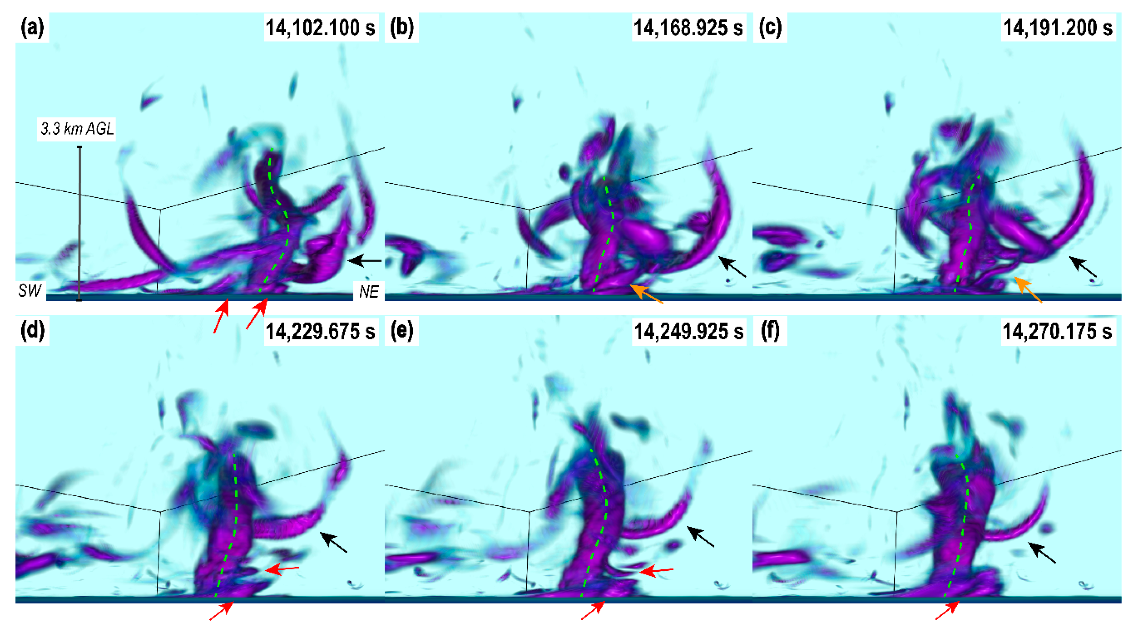
During the intensification and maintenance phases of the tornado, there is enhanced activity of HVs near its outer circulation. It is also during this phase that these structures are more prominent and well defined. This is shown in a DVR of the 3D vorticity magnitude field in Figure 5, which highlights regions of vorticity magnitude > 0.15 s−1, prior to and around the time the tornado attained EF4 strength. A supplemental video file SupVidPprtVort depicts the evolution of the vorticity magnitude field from 14,100.075 s through 14,298.000 s, when the tornado was rapidly intensifying. The general appearance of the vorticity magnitude field reveals a complex distribution of elongated vortices surrounding the tornado and its parent low-level mesocyclone. A wide spectrum of length scales is evident that includes vortices of nearly the same dimensions of the tornado down to scales near the grid spacing resolvability limit. This observation is supported by videographic evidence (Figure 6), which indicates that the width of some HVs can be as small as a few meters. (Note that the width of condensation tubes should be smaller than the actual HV circulation, e.g., [47]). The broad spectrum of HV scales (as well as other small-scale vortices in Figure 5) is a reflection of the turbulent nature of the storm’s cold pool where they reside primarily, as also seen in the visualizations of Orf et al. [10].
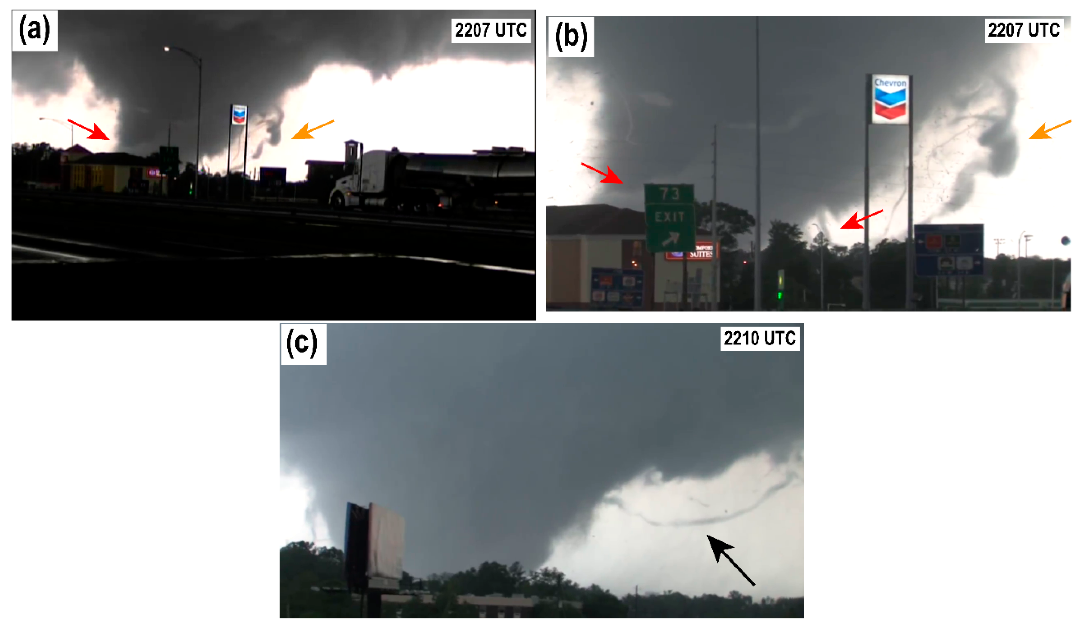
In order to assess the similarity of the simulated vorticity structure with real-world observations of HVs, Figure 6 presents visual observations from video frames of the 27 April 2011 Tuscaloosa-Birmingham EF4 tornado, when several HVs were orbiting the tornado simultaneously. In both Figure 6a,b, the storm-relative viewpoint of the observers is approximately similar to that shown in Figure 5, looking from the southeast through the RFD region, but turning north and northwest (Figure 6c) as the tornado moved northeast. In both observed and simulated tornadoes, the HVs revolve counter-clockwise in the tornadic outer wind field and tend to align azimuthally around (but outside) the tornado core, thus, forming ring-like structures encircling the tornado. Although in a different context, this behavior bears remarkable resemblance to the process by which elongated vortices in isotropic homogeneous turbulence, the so-called “worms” (e.g., [48]), interact with a large, sustained columnar vortex in the DVRs of Takahashi et al. [49]. In their study, the interaction of the sustained vortex and the worms is shown to induce disturbances in the larger vortex core flow that can affect its dynamics. Given the vorticity arrangement shown in Figure 5, it seems plausible to hypothesize that vortex-vortex interactions analogous to those shown by Takahashi et al. [49] may occur between tornadoes and surrounding HVs.
Both observed and simulated HVs have a tendency to form in preferred storm-relative regions. The majority of the vortices appear or become well defined (as large tubes in Figure 5 or condensation funnels in Figure 6) to the rear (south and southeast) and right (east) sides of the tornadoes as they ascend in the outer circulation updraft. In fact, many HVs first appear close the ground in an arc extending from rear through right side of the tornado. This is seen in the convoluted vorticity distribution surrounding the simulated tornado (Figure 5a–c) and in the large, ascending vortex attached to the right flank of the observed Tuscaloosa tornado condensation funnel, shown in the leftmost arrows in Figure 6a,b.
The evolution of HVs shown in Figure 5 and in SupVidPprtVort highlights the diversity of structures and shapes the HVs can assume when interacting with the tornado. Large HVs close to the tornado initially tend to maintain their tornado-relative position (bottommost red arrow in Figure 5e and leftmost red arrows in Figure 6a,b), then eventually become detached from the surface as they are tilted by the updraft and finally spiral and evolve into complex shapes (e.g., uppermost red arrow in Figure 5e). Smaller vortices near the tornado edge, on the other hand, are rapidly captured in the tornado outer circulation and spiral upward, either maintaining their horizontal orientation or becoming severely distorted into a variety of shapes. Two such examples of complex shapes include the coil spring and U-shaped vortices in the forward sector of the tornado in Figure 5b,c and Figure 6a,b, denoted by the orange and black arrows, respectively. Clearly, the strong vertical motion gradients in the leading edge of the tornado (especially in forward-tilted tornadoes, as in both observed and simulated tornadoes presented here) and sinking motion ahead it must be involved in the creation of these highly-distorted vortex shapes (this aspect is further discussed later). We also note that vortices located farther away from the tornado core tend to be moved around with less change in shape or orientation (e.g., the U-shaped vortex in Figure 5d–f and Figure 6c). This suggests that the rate of distortion of HVs is a function of the 3D shear strain rate surrounding the tornado core. Therefore, the length scale of the HVs and their distance to the parent tornado are both key to determining how their shapes and structures evolve near the tornadic wind field.
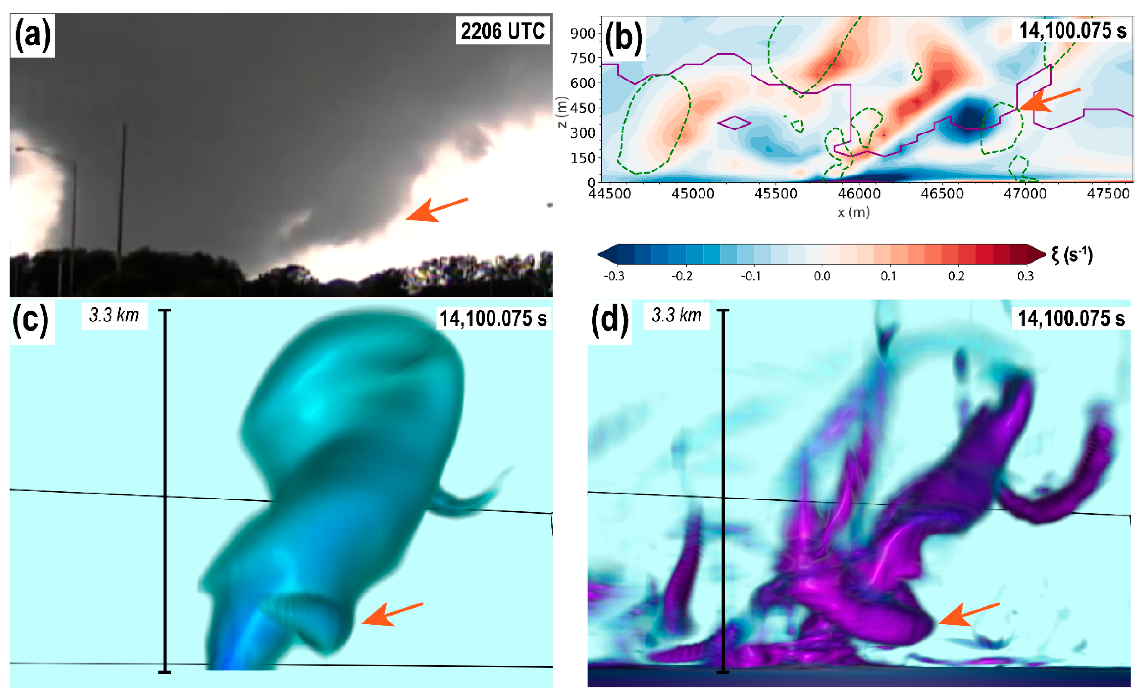
The behavior of the most prominent HV in the simulation, i.e., the one highlighted by the black arrow in Figure 5, is further compared with visual observations in Figure 7. In the real Tuscaloosa tornado, a large HV is tilted upward in the right flank of the tornado as it revolves around it and then attaches to the cloud base in its forward flank (Figure 7a). A vertical cross section along the y-axis at 14,100.075 s in the simulation (Figure 7b) reveals the corresponding HV already located in the front sector of the tornadic circulation with horizontal vorticity predominantly oriented along the x-direction. In that sector, a lowering in the cloud base can be seen collocated with the HV. Although HVs are crudely resolved in the simulation, condensation driven by cyclostrophic pressure drop is still able to form when the HV nears the cloud base because of the near-saturation air at that level. The simulated perturbation pressure (Figure 7c) and vorticity magnitude (Figure 7d) fields bear a striking resemblance with the visual observation in Figure 7a, despite the more evident horizontal orientation of the HV in the simulation fields. The region where the HV attaches to the tornado in the perturbation pressure field (Figure 7c; the evolution of the perturbation pressure field from 14,100.075 s through 14,298.000 s is shown in supplemental video SupVidPprtVort) denotes a region where the upward tilting of the HV is reduced or even slightly tilted downward ahead of the tornado in the vorticity magnitude field (Figure 7d). Such reduced upward (or downward) tilt appears to be due to weaker updraft or downward motion in the secondary vertical circulation ahead of the tornadic circulation where the HV resides which, in this case, is enhanced by the pronounced northeastward tilt of the tornado. Thus, as this particular HV rotates around the tornado, it is affected by a minimum in upward motion (or downdraft) ahead of the tornado (i.e., along the tornado motion vector) and stronger updrafts at its northwestern and southeastern tips (transverse to the tornado motion vector; see Figure 4e). This pattern of horizontal gradient of vertical motion (∇hw) may result in the U-shape of the HV later in its life cycle (Figure 5b–e and Figure 6c).
The general evolution of the HV shown in Figure 7 also suggests that, once the HV reaches the regions of strong ∇hw ahead of the tilted tornado, it aligns perpendicularly to ∇hw and attaches to this region. Ultimately, the HV becomes part of the horizontal vorticity field associated with the tornado-relative ∇hw. This does not occur for weak, small HVs: as previously stated, they are quickly distorted by the strong velocity gradients as they approach the tornado outer edge. Therefore, the visualizations indicate that strong HVs can form far outside the tornado core via processes, such as frictional or baroclinic torques, and eventually become embedded in regions of sharp tornado-relative ∇hw and attendant horizontal vorticity field.
4.2. Near-Ground Flow Kinematics and Potential HV Formation Mechanisms
Having analyzed the structure and types of HVs presented in the simulation, a brief assessment of the near-ground wind field surrounding the tornado and its associated horizontal vorticity is now presented. Even though vorticity budget analysis are not carried out in this study, the near-ground kinematic patterns around the tornado can provide valuable information about potential HV formation mechanisms and help guide future dynamical analyses.
As discussed earlier, among the variety of vortices observed in the simulation, a group of HVs is known to form near the ground in two key regions: in a circle around the base of the tornado and in an arc extending from rear through the right flanks of the tornado. The vortices near the base of the tornado continuously form and rapidly rise just outside the tornado core flow, while the ones in the rear and right flanks form longer near-surface tubes before accelerating toward the right side of the tornado and revolving around it, as previously described. One of the potential mechanisms for the rapid generation of HVs is via the Leibovich and Stewartson [50] instability. (An in-depth discussion of this mechanism can be found in Nolan [51].) Regardless of the genesis region, what is special about this class of vortices is that they typically erupt from the near-surface pool of enhanced horizontal vorticity. This shallow pool of horizontal vorticity that exists close to the ground (dark purple at the ground in Figure 5) is a direct result of surface drag and the resulting large near-surface vertical shear [11,13,14]. The tornado acts as a pump pulling the near-surface horizontal vorticity field upward: the vortices near the base of the tornado are abruptly displaced and/or tilted upward by the updraft while the ones in the right and rear flanks rise more gently along slantwise paths.
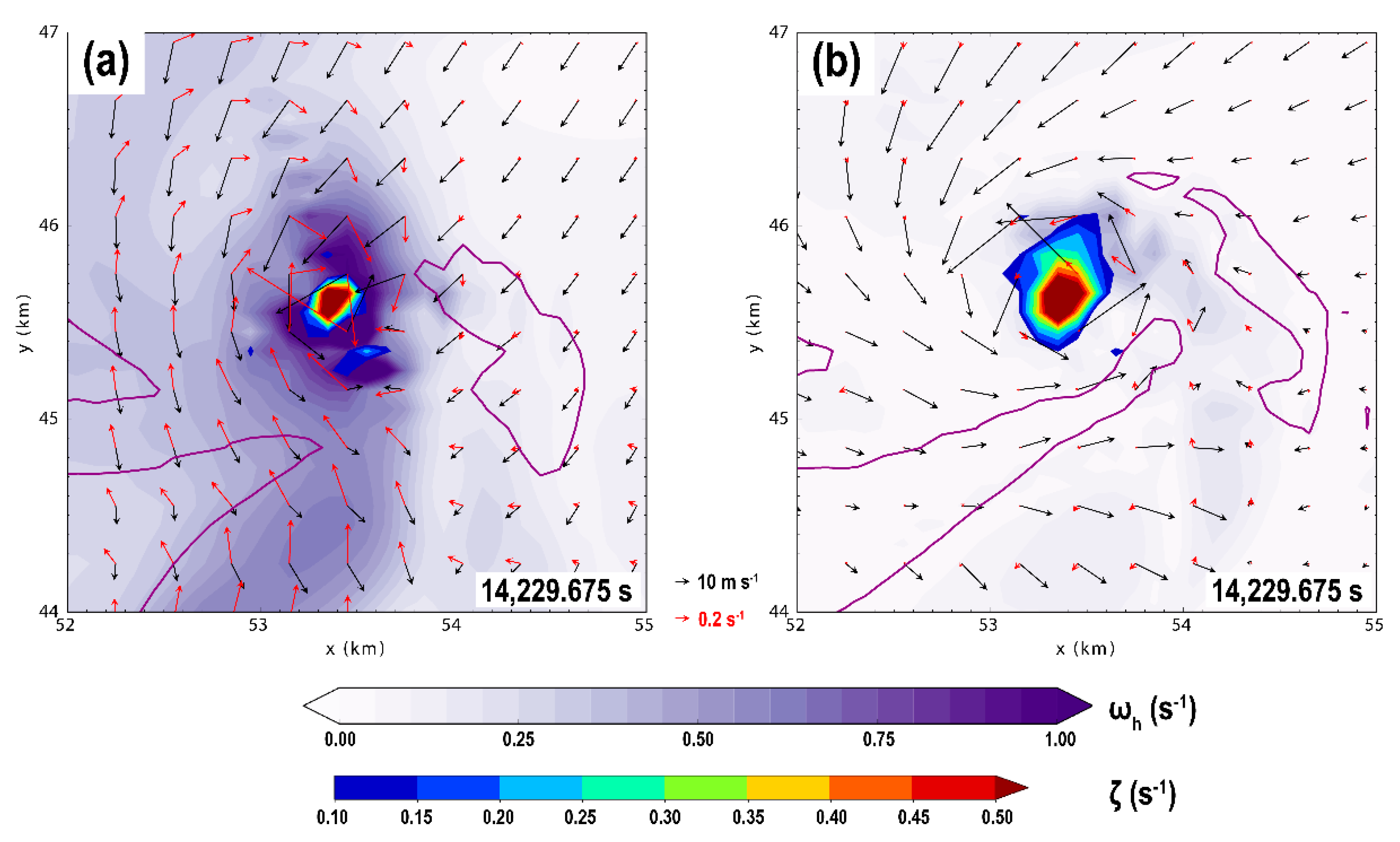
The idea that surface drag can be responsible for the generation of HVs can be linked to the predominant sense of rotation displayed by the vortices. In our 3D visualizations, virtually all large HVs, either embedded in the tornado outer circulation or RFD outflow, rotate around a horizontal axis with sinking motion ahead of them and trailing rising motion, as they orbit the tornado in the same way the HV presented by Houser et al. [9]. An analysis of the videos presented in Figure 5 also shows that the observed vortices in the Tuscaloosa tornado (as well as other tornado events, e.g., [7,8,9]) consistently display the same behavior. This suggests that HVs near the surface have horizontal vorticity vectors that point to the left of the horizontal wind vector at large angles, implying considerable crosswise horizontal vorticity [11,13,14,52]. This can be seen in Figure 8a, which shows the horizontal vorticity field at 1 m and 158 m AGL. Immediately outside the tornado core, in predominantly rotational flow, near-surface horizontal vorticity vectors, consistent with the near-surface HVs, point to the left of the prevailing horizontal wind in which they are embedded, thus having a large crosswise component. Above the surface (i.e., farther from the lower boundary; Figure 8b) the vorticity vectors become more streamwise, suggesting that HVs that arise from the near-ground pool of enhanced horizontal vorticity tend to exchange their crosswise vorticity into the streamwise direction, as they spiral around and upward near the tornado. This observation is consistent with generation of crosswise horizontal vorticity via surface friction in strong, accelerating horizontal flow [9,11,13,52].
Another possibility for the horizontal vorticity of near-surface HVs is generation by baroclinic torques [15,24,34,35,36,37,43,45]. However, if the horizontal vorticity in the HVs were mainly created baroclinically at the leading edge of a negatively buoyant RFD, the generated horizontal vorticity would point to the right of the downdraft and cold pool flows, giving an opposite sense of rotation than observed [5,43]. Yet baroclinity can still yield the observed vorticity if it is produced at the leading edge of an RFD warm surge, as suggested by Houser et al. [9]. Also vorticity thus generated should not be confined to be very close to the ground surface. This aspect is an important difference between Orf et al. [10] and the present study since the former employed a free-slip lower boundary condition while we include surface drag to capture the effects of surface frictional generation of horizontal vorticity. Recent studies [11,13,52] have found that surface-friction-generated vorticity can be an important or dominant source of vorticity the feeds a tornado vortex near the ground. This process is likely the main source of vorticity of the HVs observed in this study. More quantitative analyses of the simulation data will be needed to answer this question with any degree of certainty.
5. Discussion and Concluding Remarks
An idealized numerical simulation of a tornadic supercell is produced with the ARPS model at a tornado-resolving resolution and visualized with VAPOR; the data are analyzed, with the aid of 3D visualizations, to qualitatively determine the 3D structure, types and evolution of HVs near simulated tornadoes. The simulation includes surface drag with a semi-slip lower boundary condition in order to capture the effects of surface friction on the production of near-ground horizontal vorticity. Furthermore, the first scalar model level is placed at 1 m AGL to augment vertical resolution close to the surface to be resolve near-surface vertical shear, and to facilitate future trajectory-based analyses. The simulated parent supercell remains nontornadic during the first 3 h of life cycle, producing only mesocyclone-scale low-level vertical vorticity. After 3 h 16 min, the supercell transitions to its tornadic mode, producing two significant tornadoes. The first tornado lasts for 17 min and briefly attains EF3 strength, while maintaining EF1 winds for most of its life cycle. The second tornado is shorter lived but stronger, with peak winds reaching a high-end EF4 threshold. Both tornadoes exhibit significant tilt to the northeast with height.
HVs exist near the simulated tornadoes throughout their entire life cycle but are more prominent during the strengthening and maintenance phases of the tornadoes, consistent with the case study of Houser et al. [9]. A comparison of volume-rendered 3D vorticity magnitude fields and visual observations shows that the most significant HVs appear near the surface in an arc extending from the south toward the east sides of the tornadic circulation, embedded in both tornado outer flow and RFD outflow behind the gust front. Larger HVs tend to maintain their shape and position relative to the tornado longer than their smaller-scale counterparts, which quickly become distorted and are advected around and upward outside the tornado. Moreover, HVs farther away from the tornado tend to keep their shape and revolve around the parent circulation more slowly. This may be a result of reduced 3D shear strain rates outside and farther away from the tornado core flow. Once HVs are captured in the near-tornado, accelerating flow, very strong stretching occurs, which can occasionally form condensation inside the vortex tube via cyclostrophic pressure deficits, as shown in Figure 6 and Figure 7 and also discussed by Houser et al. [9].
A closer inspection of a strong simulated HV reveals that the vortex is advected cyclonically toward forward flank of the tornado at low levels. Because the tornado tilts forward with height, strong horizontal gradients of vertical motion exist ahead of it. Our visualizations suggest that strong HVs can form within the storm cold pool and later become attached to the zone of strong horizontal gradient of vertical motion ahead of a forward-tilted tornado. Thus, HVs can occasionally be assimilated in the horizontal vorticity field associated with tornado-relative vertical motion gradients. In fact, many of the fast moving, forward-tilted tornadoes observed on the 27 April 2011 tornado outbreak displayed HVs in their forward sectors during a significant portion of their life cycle [7].
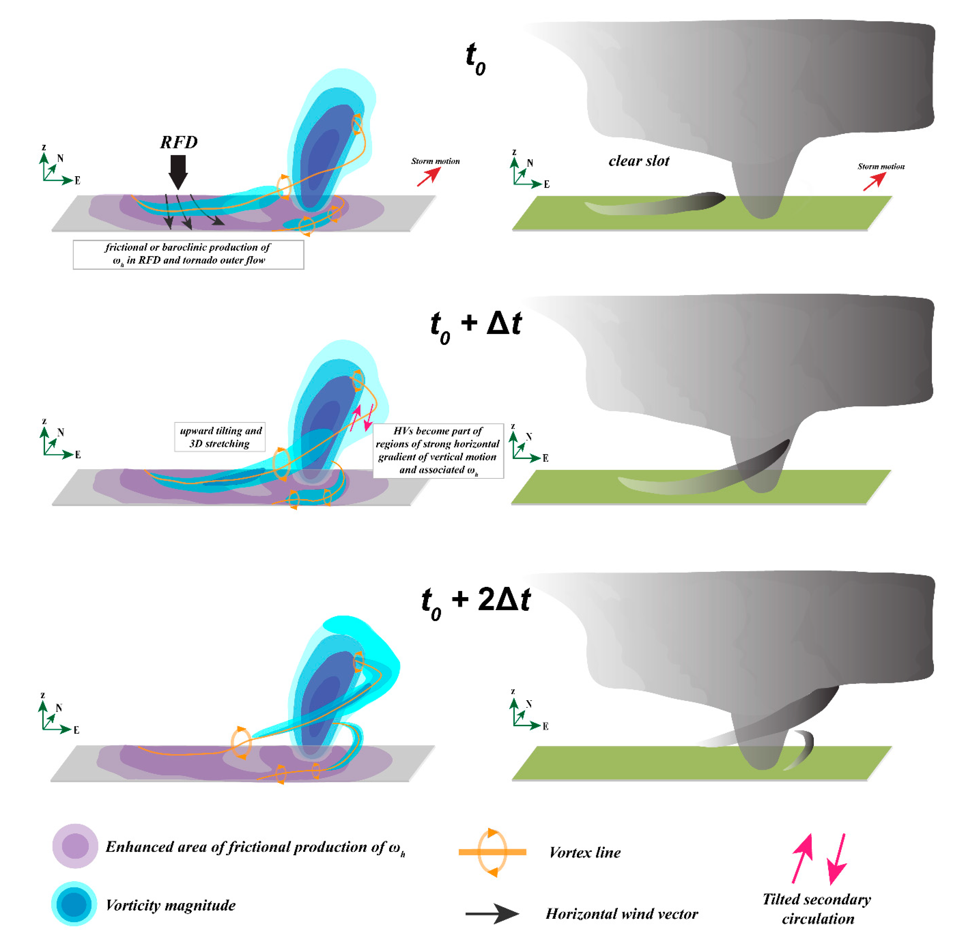
Another relevant aspect seen in both DVRs and videos of the Tuscaloosa tornado is the tendency for HVs to have horizontal vorticity vectors with a large crosswise component at low levels, similar to the 24 May 2011 El Reno tornado studied by Houser et al. [9]. Regions of large horizontal near-ground vorticity collocated with and pointing to the left of strong near-surface horizontal winds strongly suggest a possible role by surface drag in the production of HVs. Recent studies have shown that surface friction can produce significant near-ground horizontal vorticity within RFD outflows [11] and in the storm’s inflow [13,14] that is ultimately tilted and stretched to produce tornadic vortices. It may well be possible that the HVs described in this study are coherent-structure manifestations of the vorticity-generation processes discussed by Schenkman et al. [11] and Roberts et al. [13], revealed here owing to the use of 3D visualizations and comparisons with real tornado footage. Recently, 3D visualizations of simulated tornadic supercells have provided crucial insights into storm- and tornado-scale process involved in tornado formation and dynamics [10,53]. Mechanisms other than surface friction, such as baroclinity along RFD warm surges behind their primary gust fronts and reorientation of near-tornado vertical vorticity into the horizontal [9], may also be important for the generation of the variety of 3D vortex tubes in the vicinity of a tornadic wind field. The complex distribution of HVs near the simulated tornadoes in the RFD outflow suggest all these mechanisms may be acting together. A conceptual model of the 3D structure, relevant flow features and what we believe to be the most plausible mechanisms for HV formation is presented in Figure 9.
We want to point out that the 100-m horizontal grid spacing used in this study is certainly coarse to resolve the vast spectrum of HVs that may exist in nature, which possibly includes HVs of only a couple of meters of length scale. Consequently, we may be resolving only the larger, more energetic HVs in the initial portion of the inertial subrange, implying that only a small part of the HV spectrum is represented here. With an isotropic grid spacing of 30 m, Orf et al. [10] was able to resolve a broader spectrum of 3D vortical structures in their supercell’s cold pool and around the tornado. Such grid spacing was enough to allow condensation to form inside the HV as happens in nature, which suggests that, to properly address the dynamics of HVs, grid spacing on the order of a few meters is desirable.
Takahashi et al. [49] show that turbulent worm-type vortices that interact with a dominant large vortex can affect the dynamics of the latter. Although we did not address the impacts of HVs on the parent tornado itself, the interaction is clearly seen in the volume rendered movies (supplemental video). Given the highly nonlinear nature of these vortex-vortex interactions, it would be plausible to speculate that the most energetic HVs can have some influence on the tornado vortex. These questions are left for a future study that will include detailed vorticity and circulation budget analyses.
Finally, it is important to point out that the 1.5-order TKE-based subgrid-scale turbulence parameterization with a mixing length (ΔxΔyΔz)1/3 can result in relatively large vertical mixing relative to the vertical grid spacing. This would imply rather large vertical turbulence mixing and more efficient transfer of (negative) surface momentum flux (due to surface drag) upward into the flow above ground. The subgrid-scale turbulence parameterization near a rigid wall [54] and with a large grid aspect ratio ([19,55]) are issues that can potentially affect near-ground tornado dynamics and deserve further investigation.
Supplementary Materials
The following are available online at https://www.mdpi.com/2073-4433/10/11/716/s1.
Author Contributions
Conceptualization, M.I.O. and M.X.; methodology, M.I.O., M.X., L.J.W. and, B.J.R.; software, B.J.R., M.I.O. and M.X.; validation, M.I.O., M.X., L.J.W., B.J.R., N.Y.; formal analysis, M.I.O., M.X., B.J.R., L.J.W.; investigation, M.I.O. and M.X.; resources, M.I.O. and M.X.; data curation, M.I.O., B.J.R., and N.Y.; writing—original draft preparation, M.I.O.; writing—review and editing, M.I.O., L.J.W., B.J.R., M.X., and N.Y.; visualization, M.I.O. and B.J.R.; supervision, M.X. and L.J.W.; project administration, M.X., M.I.O., and L.J.W.; funding acquisition, M.X. and M.I.O.
Funding
The first author is supported by the Coordenação de Aperfeiçoamento de Pessoal de Nível Superior (CAPES), Grant number 88881.129505/2016-01 of the “Programa de Doutorado Pleno no Exterior” (DPE – 3830) under the Brazilian Ministry of Education. The second author is supported NSF Grant AGS-1261776 and NOAA VORTEX-SE Grant NA17OAR4590188.
Acknowledgments
The first author thanks CAPES by the scholarship funding provided for the development of his PhD research. The numerical experiments were conducted at the Texas Advanced Supercomputing Center (TACC), an NSF XSEDE facility. Figure 6a and Figure 7a were courtesy of Mike Wilhelm and Figure 6b,c are credited to John Brown, with permission generously granted by Kory Hartman at SevereStudios.com. Numerous discussions with Ernani L. Nascimento, Alan Shapiro, Derek Stratman, and Keith Brewster (to name a few) were very beneficial to the present study. ARPS support provided by Nathan Snook and Timothy Supinie is acknowledged. Scott Pearse from NCAR is thanked for his support with VAPOR. Lastly, the authors are grateful to the editor (Leigh Orf) and three anonymous reviewers for their constructive comments and suggestions, which led to the improvement of the manuscript.
Conflicts of Interest
The authors declare no conflict of interest.
References
- Brandes, E.A. Vertical Vorticity Generation and Mesocyclone Sustenance in Tornadic Thunderstorms: The Observational Evidence. Mon. Weather Rev. 1984, 112, 2253–2269. [Google Scholar] [CrossRef]
- Wakimoto, R.M.; Cai, H.; Murphey, H.V. The Superior, Nebraska, Supercell During BAMEX. Bull. Am. Meteorol. Soc. 2004, 85, 1095–1106. [Google Scholar] [CrossRef]
- Fujita, T.T. Tornadoes and Downbursts in the Context of Generalized Planetary Scales. J. Atmos. Sci. 1981, 38, 1511–1534. [Google Scholar] [CrossRef]
- Fiedler, B. The suction vortices and spiral breakdown in numerical simulations of tornado-like vortices. Atmos. Sci. Let. 2009, 10, 109–114. [Google Scholar] [CrossRef]
- Wurman, J.; Kosiba, K. Finescale Radar Observations of Tornado and Mesocyclone Structures. Weather Forecast. 2013, 28, 1157–1174. [Google Scholar] [CrossRef]
- Bluestein, H.B.; Weiss, C.C.; French, M.M.; Holthaus, E.M.; Tanamachi, R.L.; Frasier, S.; Pazmany, A.L. The Structure of Tornadoes near Attica, Kansas, on 12 May 2004: High-Resolution, Mobile, Doppler Radar Observations. Mon. Weather Rev. 2007, 135, 475–506. [Google Scholar] [CrossRef]
- Knupp, K.R.; Murphy, T.A.; Coleman, T.A.; Wade, R.A.; Mullins, S.A.; Schultz, C.J.; Schultz, E.V.; Carey, E.; Sherrer, A.; McCaul, E.W., Jr.; et al. Meteorological Overview of the Devastating 27 April 2011 Tornado Outbreak. Bull. Amer. Meteorol. Soc. 2014, 95, 1041–1062. [Google Scholar] [CrossRef]
- Bai, L.; Meng, Z.; Huang, L.; Yan, L.; Li, Z.; Mai, X.; Huang, Y.; Yao, D.; Wang, X. An Integrated Damage, Visual, and Radar Analysis of the 2015 Foshan, Guangdong, EF3 Tornado in China Produced by the Landfalling Typhoon Mujigae (2015). Bull. Amer. Meteor. Soc. 2017, 98, 2619–2640. [Google Scholar] [CrossRef]
- Houser, J.L.; Bluestein, H.B.; Snyder, J.C. A Finescale Radar Examination of the Tornadic Debris Signature and Weak-Echo Reflectivity Band Associated with a Large, Violent Tornado. Mon. Weather Rev. 2016, 144, 4101–4130. [Google Scholar] [CrossRef]
- Orf, L.; Wilhelmson, R.; Lee, B.; Finley, C.; Houston, A. Evolution of a Long-Track Violent Tornado within a Simulated Supercell. Bull. Amer. Meteorol. Soc. 2017, 98, 45–68. [Google Scholar] [CrossRef]
- Schenkman, A.D.; Xue, M.; Hu, M. Tornadogenesis in a High-Resolution Simulation of the 8 May 2003 Oklahoma City Supercell. J. Atmos. Sci. 2014, 71, 130–154. [Google Scholar] [CrossRef]
- Xue, M.; Hu, M.; Schenkman, A.D. Numerical prediction of 8 May 2003 Oklahoma City Tornadic Supercell and Embedded Tornado using ARPS with the Assimilation of WSR-88D data. Weather Forecast. 2014, 29, 39–62. [Google Scholar] [CrossRef]
- Roberts, B.; Xue, M.; Schenkman, A.D.; Dawson, D.T. The Role of Surface Drag in Tornadogenesis within an Idealized Supercell Simulation. J. Atmos. Sci. 2016, 73, 3371–3395. [Google Scholar] [CrossRef]
- Roberts, B.; Xue, M. The Role of Surface Drag in Mesocyclone Intensification Leading to Tornadogenesis within an Idealized Supercell Simulation. J. Atmos. Sci. 2017, 74, 3055–3077. [Google Scholar] [CrossRef]
- Davies-Jones, R.; Trapp, R.J.; Bluestein, H.B. Tornadoes and tornadic storms. In Severe Convective Storms; Meteorological Monographs; American Meteorological Society: Boston, MA, US, 2001; pp. 167–221. [Google Scholar]
- Clyne, J.; Mininni, P.; Norton, A.; Rast, M. Interactive desktop analysis of high resolution simulations: Application to turbulent plume dynamics and current sheet formation. New J. Phys. 2007, 9, 301. [Google Scholar] [CrossRef]
- Li, S.; Jaroszynski, S.; Pearse, S.; Orf, L.; Clyne, J. VAPOR: A Visualization Package Tailored to Analyze Simulation Data in Earth System Science. Atmosphere 2019, 10, 488. [Google Scholar] [CrossRef]
- Xue, M.; Droegemeier, K.K.; Wong, V. The Advanced Regional Prediction System (ARPS)—A multiscale nonhydrostatic atmospheric simulation and prediction model. Part I: Model dynamics and verification. Meteor. Atmos. Phys. 2000, 75, 161–193. [Google Scholar] [CrossRef]
- Xue, M.; Droegemeier, K.K.; Wong, V.; Shapiro, A.; Brewster, K.; Carr, F.; Weber, D.; Liu, Y.; Wang, D. The Advanced Regional Prediction System (ARPS)—A multiscale nonhydrostatic atmospheric simulation and prediction tool. Part II: Model physics and applications. Meteor. Atmos. Phys. 2001, 76, 143–165. [Google Scholar] [CrossRef]
- Xue, M.; Wang, D.H.; Gao, J.D.; Brewster, K.; Droegemeier, K.K. The Advanced Regional Prediction System (ARPS), storm-scale numerical weather prediction and data assimilation. Meteor. Atmos. Phys. 2003, 82, 139–170. [Google Scholar] [CrossRef]
- Vande Guchte, A.; Dahl, J.M.L. Sensitivities of Parcels Trajectories beneath the Lowest Scalar Model Level of a Lorenz Vertical Grid. Mon. Weather Rev. 2018, 146, 1427–1435. [Google Scholar] [CrossRef]
- Lin, Y.L.; Farley, R.D.; Orville, H.D. Bulk Parameterization of the Snow Field in a Cloud Model. J. Appl. Clim. Meteor. 1983, 22, 1065–1092. [Google Scholar] [CrossRef]
- Snook, N.; Xue, M. Effects of microphysical drop size distribution on tornadogenesis in supercell thunderstorms. Geophys. Res. Lett. 2008, 35, 851–854. [Google Scholar] [CrossRef]
- Dawson, D.T.; Xue, M.; Milbrandt, J.A.; Yau, M.K. Comparison of Evaporation and Cold Pool Development between Single-Moment and Multimoment Bulk Microphysics Schemes in Idealized Simulations of Tornadic Thunderstorms. Mon. Weather Rev. 2010, 138, 1152–1171. [Google Scholar] [CrossRef]
- Moeng, C.H.; Wyngaard, J.C. Spectral Analysis of Large-Eddy Simulations of the Convective Boundary Layer. J. Atmos. Sci. 1988, 45, 3573–3587. [Google Scholar] [CrossRef]
- Yussouf, N.; Dowell, D.C.; Wicker, L.J.; Knopfmeier, K.H. Storm-Scale Data Assimilation and Ensemble Forecasts for the 27 April 2011 Severe Weather Outbreak in Alabama. Mon. Weather Rev. 2015, 143, 3044–3066. [Google Scholar] [CrossRef]
- Karstens, C.D.; Gallus, W.A., Jr.; Lee, B.D.; Finley, C.A. Analysis of Tornado-Induced Tree Fall Using Aerial Photography from the Joplin, Missouri, and Tuscaloosa–Birmingham, Alabama, Tornadoes of 2011. J. Appl. Clim. Meteor. 2013, 52, 1049–1068. [Google Scholar] [CrossRef]
- Potvin, C.K.; Elmore, K.L.; Weiss, S.J. Assessing the Impacts of Proximity Sounding Criteria on the Climatology of Significant Tornado Environments. Weather Forecast. 2010, 25, 921–930. [Google Scholar] [CrossRef]
- Blumberg, W.; Halbert, K.; Supinie, T.; Marsh, P.; Thompson, T.; Hart, J. SHARPpy: An Open Source Sounding Analysis Toolkit for the Atmospheric Sciences. Bull. Am. Meteorol. Soc. 2017, 98, 1625–1636. [Google Scholar] [CrossRef]
- Roberts, B.J. The Role of Surface Drag in Supercell Tornadogenesis and Mesocyclonegenesis: Studies Based on Idealized Numerical Simulations. Ph.D. Thesis, University of Oklahoma, Norman, OK, USA, 2017. [Google Scholar]
- Dawson, D.T.; Roberts, B.; Xue, M. A Method to Control the Environmental Wind Profile in Idealized Simulations of Deep Convection with Surface Friction. Mon. Weather Rev. 2019, 147, 3935–3954. [Google Scholar] [CrossRef]
- Skamarock, W.C.; Klemp, J.B. The Stability of Time-Split Numerical Methods for the Hydrostatic and the Nonhydrostatic Elastic Equations. Mon. Weather Rev. 1992, 147, 2109–2127. [Google Scholar] [CrossRef]
- Xue, M.; Droegemeier, K.K.; Wong, V.; Shapiro, A.; Brewster, K. ARPS user’s guide, version 4.0. Center for Analysis and Prediction of Storms. Ph.D. Thesis, University of Oklahoma, Norman, OK, USA, 1995; p. 380. [Google Scholar]
- Adlerman, E.J.; Droegemeier, K.K. The Dependence of Numerically Simulated Cyclic Mesocyclonegenesis upon Environmental Vertical Wind Shear. Mon. Weather Rev. 2005, 133, 3595–3623. [Google Scholar] [CrossRef] [Green Version]
- Beck, J.; Weiss, C. An Assessment of Low-Level Baroclinicity and Vorticity within a Simulated Supercell. Mon. Weather Rev. 2013, 141, 649–669. [Google Scholar] [CrossRef]
- Dahl, J.M.L.; Parker, M.D.; Wicker, L.J. Imported and Storm-Generated Near-Ground Vertical Vorticity in a Simulated Supercell. J. Atmos. Sci. 2014, 71, 3027–3051. [Google Scholar] [CrossRef]
- Parker, M.D.; Dahl, J.M.L. Production of Near-Surface Vertical Vorticity by Idealized Downdrafts. Mon. Weather Rev. 2015, 143, 2795–2816. [Google Scholar] [CrossRef]
- Coffer, B.E.; Parker, M.D. Simulated Supercells in Nontornadic and Tornadic VORTEX2 Environments. Mon. Weather Rev. 2017, 145, 149–180. [Google Scholar] [CrossRef]
- Griffin, C.B.; Bodine, D.J.; Kurdzo, J.M.; Mahre, A.; Palmer, R.D. High-Temporal Resolution Observations of the 27 May 2015 Canadian, Texas, Tornado Using the Atmospheric Imaging Radar. Mon. Weather Rev. 2019, 147, 873–891. [Google Scholar] [CrossRef]
- Fujita, T.T.; Bradbury, D.L.; Van Thullenar, C.F. Palm Sunday Tornadoes of April 11, 1965. Mon. Weather Rev. 1970, 98, 29–69. [Google Scholar] [CrossRef]
- Dowell, D.C.; Bluestein, H.B. The 8 June 1995 McLean, Texas, storm. Part I: Observations of cyclic tornadogenesis. Mon. Weather Rev. 2002, 130, 2626–2648. [Google Scholar] [CrossRef]
- French, M.M.; Kingfield, D.M. Dissipation Characteristics of Tornadic Vortex Signatures Associated with Long-Duration Tornadoes. J. Appl. Clim. Meteor. 2019, 58, 317–339. [Google Scholar] [CrossRef] [Green Version]
- Markowski, P.M.; Richardson, Y.; Rasmussen, E.; Straka, J.; Davies-Jones, R.; Trapp, R.J. Vortex lines within low-level mesocyclones obtained from pseudo-dual-Doppler radar observations. Mon. Weather Rev. 2008, 136, 3513–3535. [Google Scholar] [CrossRef] [Green Version]
- Bluestein, H.B.; French, M.M.; Snyder, J.C.; Houser, J.B. Doppler radar observations of anticyclonic tornadoes in cyclonically rotating, right-moving supercells. Mon. Weather Rev. 2016, 144, 1591–1616. [Google Scholar] [CrossRef]
- Adlerman, E.J.; Droegemeier, K.K.; Davies-Jones, R. A numerical simulation of cyclic mesocyclogenesis. J. Atmos. Sci. 1999, 56, 2045–2069. [Google Scholar] [CrossRef]
- Lemon, L.R.; Doswell, C.A. Severe Thunderstorm Evolution and Mesocyclone Structure as Related to Tornadogenesis. Mon. Weather Rev. 1979, 107, 1184–1197. [Google Scholar] [CrossRef]
- Atkins, N.T.; Butler, K.M.; Flynn, K.R.; Wakimoto, R.M. 2014: An integrated damage, visual, and radar analysis of the 2013 Moore, Oklahoma, EF5 tornado. Bull. Amer. Meteor. Soc. 2014, 95, 1549–1561. [Google Scholar] [CrossRef]
- Jiménez, J.; Wray, A.A.; Saffman, P.G.; Rogallo, R.S. The structure of intense vorticity in isotropic turbulence. J. Fluid Mech. 1993, 255, 65–90. [Google Scholar] [CrossRef] [Green Version]
- Takahashi, N.; Ishii, H.; Miyazaki, T. The influence of turbulence on a columnar vortex. Phys. Fluids 2005, 17, 035105. [Google Scholar] [CrossRef]
- Leibovich, S.; Stewartson, K. A sufficient condition for the instability of columnar vortices. J. Fluid Mech. 1983, 126, 335–356. [Google Scholar] [CrossRef]
- Nolan, D.S. Three-dimensional instabilities in tornado-like vortices with secondary circulations. J. Fluid Mech. 2012, 711, 61–100. [Google Scholar] [CrossRef] [Green Version]
- Yokota, S.; Niino, H.; Seko, H.; Kunii, M.; Yamauchi, H. Important Factors for Tornadogenesis as Revealed by High-Resolution Ensemble Forecasts of the Tsukuba Supercell Tornado of 6 May 2012 in Japan. Mon. Weather Rev. 2018, 146, 1109–1132. [Google Scholar] [CrossRef]
- Orf, L. A Violently Tornadic Supercell Thunderstorm Simulation Spanning a Quarter-Trillion Grid Volumes: Computational Challenges, I/O Framework, and Visualizations of Tornadogenesis. Atmosphere 2019, 10, 578. [Google Scholar] [CrossRef] [Green Version]
- Chow, F.K.; Street, R.L.; Xue, M.; Ferziger, J.H. Explicit Filtering and Reconstruction of Turbulence Modeling for Large-Eddy Simulation of Neutral Boundary Layer Flow. J. Atmos. Sci. 2005, 62, 2058–2077. [Google Scholar] [CrossRef] [Green Version]
- Nishizawa, S.; Yashiro, H.; Sato, Y.; Miyamoto, Y.; Tomita, H. Influence of grid aspect ratio on planetary boundary layer turbulence in large-eddy simulations. Geosci. Model Dev. 2015, 8, 3393–3419. [Google Scholar] [CrossRef] [Green Version]
Figure 1.
(a) Skew T-logp diagram of the thermodynamic profile defining the storm environment. The red and green lines represent the temperature and dew-point temperature profiles, respectively, both in °C. The black dashed line indicates a parcel that ascends pseudo adiabatically from the surface. (b) Environmental hodograph of storm-relative winds averaged over a 0.2° × 0.2° latitude-longitude box centered over Tuscaloosa. The green arrow denotes the ground-relative storm motion vector that has been subtracted from the wind profile. Some relevant convective parameters are shown below the figures. The sounding and convective parameters were produced using the Sounding and Hodograph Analysis and Research Program in Python (SHARPpy) software [29].

Figure 2.
Select stages of the simulated supercell life cycle. (a) 3600.000 s, (b) 7200.000 s, (c) 10,800.000 s, (d) 11,888.775 s, (e) 12,032.550 s, (f) 12,929.625 s, (g) 13,950.225 s, (h) 14,274.000 s, and (i) 14,608.000 s. Vertical vorticity (light shading; s−1), horizontal wind (vectors; m s−1), and the 0.3 g kg−1 rainwater mixing ratio contour. Vertical vorticity rivers (VVR, in (d)) are denoted by green arrows in (d)–(i). Pockets of strong vertical vorticity associated with the tornadoes in the center of the domain are shaded in the foreground, starting at 0.1 s−1. All fields at 158 m AGL.

Figure 3.
(a)–(f) DVR of vertical vorticity with values greater (less) than 0.075 s−1 (−0.075 s−1) indicating regions of cyclonic (anticyclonic) rotation in yellow (blue). Buoyancy (B; in m s−1) is displayed at 1 m AGL, with positively or neutrally (negatively) buoyant air in green (blue). The life cycle of the first tornado is shown at (a) 11,888.775 s (tornadogenesis), (b) 12,032.550 s (peak stage), and (c) 12,929.625 s (demise). (d)–(f) Same as in (a)–(c), but for the second tornado at (d) 13,950.225 s, (e) 14,274.000 s, and (f) 14,608.000 s. (g)–(i) The cloud field (sum of cloud water and cloud ice mixing ratios; in g kg−1) corresponding to the second tornado in (d)–(f). All nonzero values are displayed.

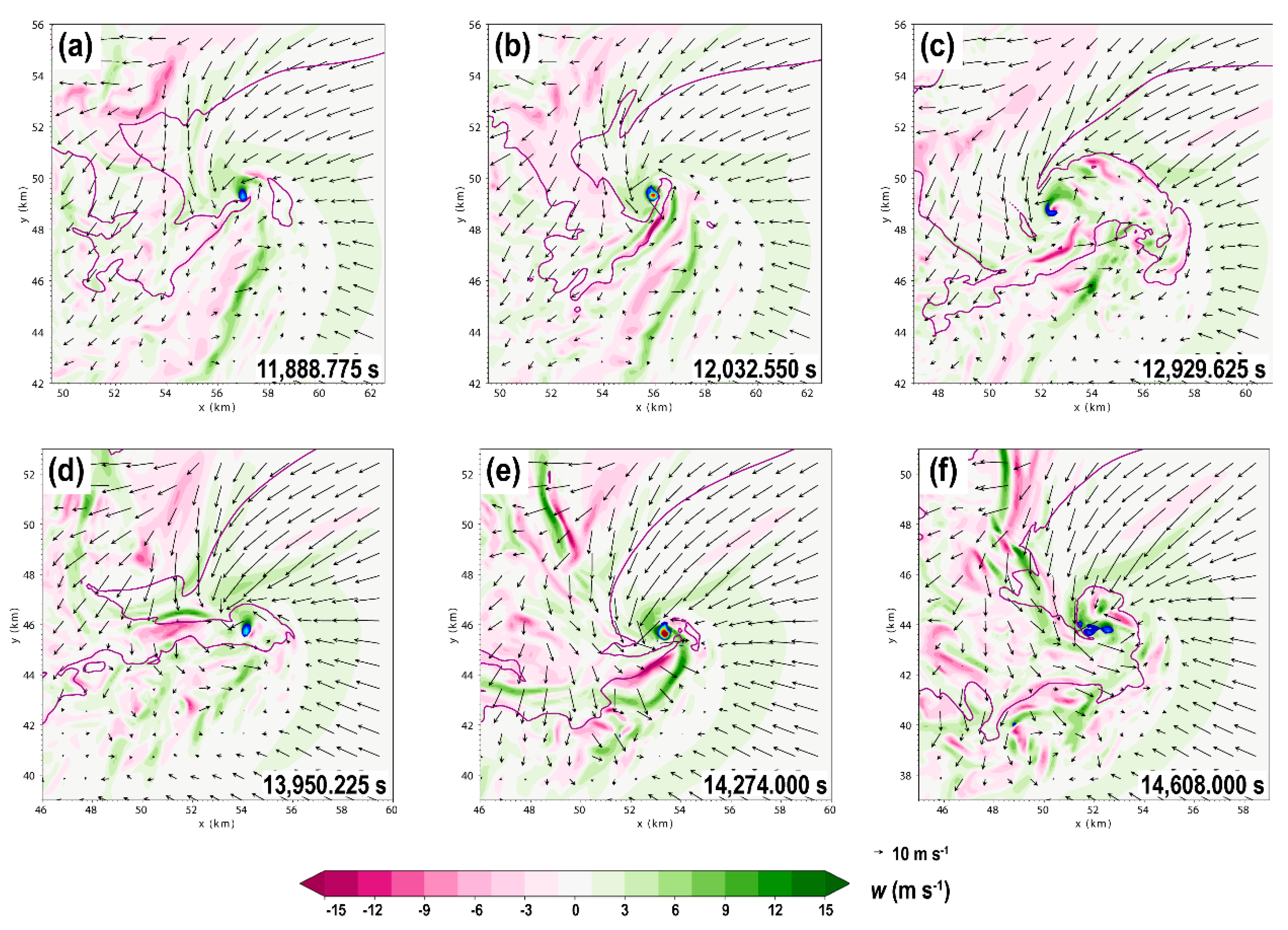
Figure 4.
Vertical velocity field (light shading; m s−1) throughout the life cycle of the simulated tornadoes at (a) 11,888.775 s, (b) 12,032.550 s, (c) 12,929.625 s, (d) 13,950.225 s, (e) 14,274.000 s, and (f) 14,608.000 s (compare with Figure 2d–i and Figure 3a–i). Horizontal wind (vectors; m s−1) and the 0.3 g kg−1 rainwater mixing ratio contour are also plotted. Pockets of strong vertical vorticity associated with the tornadoes in the center of the domain are shaded in the foreground, starting at 0.1 s−1. All fields at 158 m AGL.

Figure 5.
DVR of vorticity magnitude, highlighting values greater than 0.15 s−1, at select time frames: (a) 14,102.100 s, (b) 14,168.925 s, (c) 14,191.200 s, (d) 14,229.675 s, (e) 14,249.925 s, and (f) 14,270.175 s. The view point is that of an observer located at the southeast corner of the domain, looking toward the northwest corner. The green dashed line denotes the tornado vortex axis. Red arrows indicate vortices that form around the tornado and surrounding RFD outflow at the surface. Orange and black arrows indicate distinct vortices used for comparison with real vortices in Figure 6.

Figure 6.
Visual observations of the 27 April 2011 Tuscaloosa tornado displaying several HVs. Video frames extracted from videos of (a) Mike Wilhelm (available online at: https://www.youtube.com/watch?v=T0FHTG9VETY) and (b) John Brown (available online at: https://www.youtube.com/watch?v=9KjWtBrEYHY), courtesy of Mike Wilhelm and Kory Hartman at SevereStudios.com, respectively. Red, orange and black arrows indicate key vortices discussed in the text. Other vortices are also evident in the figure. Tornado motion is due northeast (from left to right in the figure). Times in UTC are estimated.

Figure 7.
Tilting of HVs in the forward flank of tornadoes. (a) Visual observations of the 27 April 2011 Tuscaloosa tornado at 2206 UTC (extracted from Mike Wilhelm’s video, available online at: https://www.youtube.com/watch?v=T0FHTG9VETY; courtesy of M. Wilhelm). (b) Vertical cross section of x-vorticity component (ξ; shaded in s−1) along x = 54.05 km. Solid purple contours denote the 1 × 10⁻³ g kg−1 cloud water mixing ratio isopleth and dashed green contours denote downward motion regions where w ≤ −10 m s−1. (c) DVR of perturbation pressure, highlighting values less than −9 hPa. (d) DVR of vorticity magnitude, highlighting values greater than 0.15 s−1 (as in Figure 5). The dark orange arrows indicate the position of the HV and the vertical black line indicates the scale height of the tornado in the DVRs. In all panels, the view is from the east-southeast. Tornado motion is due northeast (from left to right in the figure). All simulation fields are valid at 14,100.075 s.

Figure 8.
Horizontal vorticity (magnitude is light shaded and vectors are red; in s−1) centered at the tornado at (a) 1 m AGL and (b) 158 m AGL valid at 14,229.675 s (during the intensification phase of the tornado). Horizontal wind vectors are in black (in m s−1) and vertical vorticity ζ is shaded in the foreground, starting at 0.1 s−1. The purple line indicates the 0.3 g kg−1 rainwater mixing ratio isopleth.

Figure 9.
Conceptual model of evolution of HVs in the simulation from initial time t0 through t0 + 2∆t, at ∆t time increments. Left column: 3D vorticity magnitude isosurfaces shaded in blue. The vertically-oriented vortex represents an intensifying or mature tornado while slantwise, detached vortex tubes represent more horizontally-oriented vortices in the periphery of the tornado. Regions of enhanced frictional generation of horizontal vorticity in strong, near-ground horizontal wind embedded in the RFD outflow are shaded in purple. Magenta arrows in the middle panel show the tilted circulation on the forward side of the tornado. Representative vortex lines associated with the HVs are displayed in light orange, with circular arrows indicating their sense of rotation. Strong surface RFD flow is indicated by the curved black arrows. Right column: The cloud field associated with a tornado producing HVs consistent with the vorticity field displayed in the left column and visual observations. The RFD-related clear slot is annotated. The storm is moving to the northeast, as indicated by the red arrow the upper panel.

© 2019 by the authors. Licensee MDPI, Basel, Switzerland. This article is an open access article distributed under the terms and conditions of the Creative Commons Attribution (CC BY) license (http://creativecommons.org/licenses/by/4.0/).
Share and Cite
MDPI and ACS Style
Oliveira, M.I.; Xue, M.; Roberts, B.J.; Wicker, L.J.; Yussouf, N. Horizontal Vortex Tubes near a Simulated Tornado: Three-Dimensional Structure and Kinematics. Atmosphere 2019, 10, 716. https://doi.org/10.3390/atmos10110716
AMA Style
Oliveira MI, Xue M, Roberts BJ, Wicker LJ, Yussouf N. Horizontal Vortex Tubes near a Simulated Tornado: Three-Dimensional Structure and Kinematics. Atmosphere. 2019; 10(11):716. https://doi.org/10.3390/atmos10110716
Chicago/Turabian StyleOliveira, Maurício I., Ming Xue, Brett J. Roberts, Louis J. Wicker, and Nusrat Yussouf. 2019. "Horizontal Vortex Tubes near a Simulated Tornado: Three-Dimensional Structure and Kinematics" Atmosphere 10, no. 11: 716. https://doi.org/10.3390/atmos10110716
Note that from the first issue of 2016, this journal uses article numbers instead of page numbers. See further details here.