Temperature Prediction Using the Missing Data Refinement Model Based on a Long Short-Term Memory Neural Network
by
 ,
,
Inyoung Park
1,† ,
,
Hyun Soo Kim
2,†,
Jiwon Lee
1,
Joon Ha Kim
2,
Chul Han Song
2 and
Hong Kook Kim
1,* 1
School of Electrical Engineering and Computer Science, Gwangju Institute of Science and Technology, Gwangju 61005, Korea
2
School of Earth Sciences and Environmental Engineering, Gwangju Institute of Science and Technology, Gwangju 61005, Korea
*
Author to whom correspondence should be addressed.
†
These authors contributed equally to this work.
Atmosphere 2019, 10(11), 718; https://doi.org/10.3390/atmos10110718
Submission received: 16 October 2019
/
Revised: 4 November 2019
/
Accepted: 14 November 2019
/
Published: 16 November 2019
(This article belongs to the Special Issue Application of Statistical Methods and Machine Learning to Large-Scale Climate Informatics)
Abstract
:In this paper, we propose a new temperature prediction model based on deep learning by using real observed weather data. To this end, a huge amount of model training data is needed, but these data should not be defective. However, there is a limitation in collecting weather data since it is not possible to measure data that have been missed. Thus, the collected data are apt to be incomplete, with random or extended gaps. Therefore, the proposed temperature prediction model is used to refine missing data in order to restore missed weather data. In addition, since temperature is seasonal, the proposed model utilizes a long short-term memory (LSTM) neural network, which is a kind of recurrent neural network known to be suitable for time-series data modeling. Furthermore, different configurations of LSTMs are investigated so that the proposed LSTM-based model can reflect the time-series traits of the temperature data. In particular, when a part of the data is detected as missing, it is restored by using the proposed model’s refinement function. After all the missing data are refined, the LSTM-based model is retrained using the refined data. Finally, the proposed LSTM-based temperature prediction model can predict the temperature through three time steps: 6, 12, and 24 h. Furthermore, the model is extended to predict 7 and 14 day future temperatures. The performance of the proposed model is measured by its root-mean-squared error (RMSE) and compared with the RMSEs of a feedforward deep neural network, a conventional LSTM neural network without any refinement function, and a mathematical model currently used by the meteorological office in Korea. Consequently, it is shown that the proposed LSTM-based model employing LSTM-refinement achieves the lowest RMSEs for 6, 12, and 24 h temperature prediction as well as for 7 and 14 day temperature prediction, compared to other DNN-based and LSTM-based models with either no refinement or linear interpolation. Moreover, the prediction accuracy of the proposed model is higher than that of the Unified Model (UM) Local Data Assimilation and Prediction System (LDAPS) for 24 h temperature predictions.
1. Introduction
In the last several decades, abnormal weather, such as cold weather, heavy snow, heavy rain, and drought, has been occurring more and more frequently in all parts of the world, causing human injury and death, property damage, and health and environmental problems [1]. In other words, weather change has a direct negative impact on the daily quality of life. In particular, unexpectedly increased temperatures harm outdoor workers [2]. Temperature forecasts can be used to determine what to wear on a given day and to plan one’s work outside [3]. Depending on the applications of the temperature forecast, a suitable model should be designed at a specific site or a region with at least 10 days’ prediction [4].
Meteorological institutes usually forecast prediction results based on numerical weather prediction (NWP) models that predict the weather based on current weather conditions [5]. In general, NWP models target the forecasts for large geometrical areas, such as the East Asian region, and they are good at handling weather that is complexly connected with various factors that dynamically influence the subsequent day’s weather. However, NWP often produces biased temperatures in proportion to the increase of the local elevation and topographical complexity [6]. Moreover, predicting spatial and temporal changes in temperature for areas composed of complex topography remains a challenge to NWP models [7].
Over recent decades, to train these irregularities, deep learning models have been developed to predict weather change that involves atmospheric time series data. For example, a multi-layer perceptron (MLP) model, which is a neural network with one hidden layer, was proposed to deal with maximum ozone levels in Texas metropolitan areas [8]. Next, a three-layer deep neural network (DNN) model was proposed to predict the air pollution levels of cities in China [9]. In addition, the temperature prediction accuracy of a DNN-based model was compared with those of traditional mathematical models, and it was discovered that the DNN provided comparable accuracy and offered the advantage of including data that are not used in traditional equations [10].
Therefore, the purpose of this study is to design a temperature prediction model based on a DNN by using real observed weather data. Among different kinds of neural networks, the proposed prediction model is constructed based on a long short-term memory (LSTM) neural network, which is a type of recurrent neural network (RNN). This is because the LSTM architecture is more appropriate for weather data than a feedforward DNN or a typical RNN structure due to the time-series characteristics of weather data [11]. In order to train a deep learning model, a huge amount of training data is needed, but these data should not be defective. However, there is a limitation to collecting weather data since we are unable to measure data that have been missed. Thus, the collected data are apt to be incomplete, with random or extended gaps. Therefore, the proposed temperature prediction model incorporates a function for missing data refinement into the LSTM framework in order to restore missing weather data. The proposed model is composed of four stages. In the first stage, the model detects whether or not any component of the input data is missing. The second stage of the model training constructs an LSTM-based refinement model using all the training data. Then, the third stage of the proposed model tries to predict the temperature for the missing vector components. The last stage retrains the temperature prediction model using the refined data.
As mentioned in [4], the proposed model also aims at predicting temperature up to 14 days in advance using 24 h weather data as the input, and it can also provide 6, 12, and 24 h temperature predictions. In order to compare the performance of the proposed model, four different temperature prediction models are considered: (1) a prediction model using a DNN, (2) a prediction model using a conventional LSTM without any refinement function, (3) a prediction model using an LSTM with a simple gap-filling method by linearly interpolating missed data from past and future data, and (4) a unified model (UM), which is a mathematical model currently used by the meteorological office in Korea. Then, the performances of the different temperature prediction models are compared by measuring the root-mean-squared errors (RMSEs) between the real observed and predicted temperatures for the different models.
The remainder of this paper is organized as follows. Section 2 discusses the methodology of deep learning-based temperature prediction models. Then, Section 3 proposes an LSTM-based temperature prediction model along with the proposed refinement function. Section 4 evaluates the performance of the proposed model and compares it with that of other deep learning models and a UM model. Finally, Section 5 summarizes and concludes this paper.
2. Deep Learning-Based Temperature Prediction Models
2.1. Deep Neural Network (DNN)
Deep learning is a field of machine learning that teaches machines to think like people. Deep learning attempts a high level of abstraction from the given data through a combination of several nonlinear transformations. A number of studies have been conducted on how to express various data in a form that can be understood by machines. As a result, various deep learning models, such as DNN, convolutional neural network (CNN), RNN, and LSTM, have been developed to replace conventional signal processing techniques in many applications, including speech recognition, image recognition, event detection, and natural language processing. Figure 1a shows an example of a typical DNN. As shown in the figure, the DNN is a multi-layer artificial neural network that has at least two hidden layers between its input layer and output layer, and many hidden layers can be stacked deeper. Also, each layer has feed-forward connections between the neurons. Thus, information representation is performed by logistic functions applied to each node of each layer.
In this study, in order to compare the performance of the temperature prediction model proposed in Section 3 with that of the DNN model described in this subsection, we construct three different DNN models for temperature prediction according to different time periods, whose architecture is shown in Figure 1b, as proposed in [12]. As shown in the figure, each of the three DNN models has an input layer with 6, 12, or 24 nodes for 6, 12, or 24 h prediction, respectively. In addition, each DNN model has three hidden layers with 96 nodes per layer. The output layer has a single node whose target value is assigned as the observed temperature at the corresponding future time. As an activation function, the rectified linear unit (ReLU) [13] is applied to all the layers.
Each DNN model is implemented in the deep learning package Keras (version 2.1.6) using TensorFlow (version 1.8.0) [14]. In particular, the temperature data in degrees Celsius are first converted into degrees Kelvin, and the average temperature over all the training data is used for the initial weights of all the models with zero biases [15]. The mean square error (MSE) between the target and the predicted temperature is used as a cost function [16]. The adaptive moment estimation (Adam) optimization is utilized for the backpropagation algorithm with a learning rate of 0.01 [17]. The detailed description on the dataset as well as the prediction accuracies of the DNN models are given in Section 4.2 and Section 4.3.
2.2. Recurrent Neural Network (RNN)
In order to take advantage of the characteristics of time series data, RNNs have been proven to give state-of-the-art performance in various applications [18]. As shown in Figure 2, an RNN is capable of intrinsically handling both current and past time data, while a DNN only deals with current time data. In other words, the hidden state value, at a time step, t, can carry memory forward mathematically by using the following equation:
where , and are the inputs to the RNN, the hidden state of the previous time step, t − 1, and a weight matrix, respectively. Also, b is a bias added to the gate, and is the activation function applied for the hidden state of current time , which is fed to the next layer directly.
The structure of the RNN is more suitable for treating time-series data than that of DNN shown in Figure 1. However, an RNN needs to recurrently track previous data in its hidden states, where information from the inputs to the output is transferred through a huge number of multiplications described in Equation (1). This causes the vanishing gradient problem during model training [19].
2.3. Long Short-Term Memory (LSTM) Neural Network
LSTM neural networks are a kind of RNN developed to be able to learn longer periods of data than RNNs [20]. This is achieved by controlling the hidden state from the gates in the LSTM to solve the vanishing gradient problem. Each block of the LSTM used in this paper consists of an input gate, a forget gate, and an output gate, as shown in Figure 3a.
For a given time, t, the gates in the LSTM calculate the gate values with the input, , the previous hidden state value, , and the previous cell value, , by the following equations [21]:
where , , and are the input, forget, and output gate values, respectively, for the current time, t. In addition, is an activation function that is usually realized as the logistic sigmoid function, ranging from 0 to 1. Further, the in Equations (2)–(4) denotes the weight matrices for computing the gate values. For example, in Equation (2) is a weight matrix connecting the input, , to the input gate, . Lastly, , , and are the biases that are added to each gate in order to adjust the center of a data space according to the training data.
The LSTM cell takes a block input to decide whether it forgets the entire previous memory or ignores new input data by applying an activation function, , which is implemented by a hyperbolic tangent function. Consequently, the cell value at time t is computed as
where is a bias for the cell. That is, the memory of LSTM retains the amount of the multiplication of the previous cell value, , and the forget gate value, , as well as the partial amount of the input gate value, , controlled by .
Next, the cell value, , is used to get the hidden state value, , by applying an activation function, , to , which is also a hyperbolic tangent defined as , such as
Compared to the RNN described in the previous subsection, the LSTM has three gates that control the truncation of the length of data sequence properly, which can solve the vanishing gradient problem with small extra computational costs [22].
Figure 3b shows the architecture of a conventional LSTM neural network for temperature prediction, which consists of one input layer, two LSTM layers, and one output layer. Also, there are L hidden nodes in the model (L = 192), which is set based on exhaustive experiments. Note that, similar to the DNN models described in Section 2.1, there are three LSTM models, respectively, with 6, 12, and 24 nodes for the input layer depending on the prediction time periods (T in the figure) of 6, 12, and 24 h, respectively. In addition, each LSTM layer has one cell, as shown in Figure 3a. The training procedure and development environment of the three LSTM models are identical to those of the DNN models mentioned in Section 2.1; a detailed description of the dataset and the prediction accuracies of the DNN models will be also given in Section 4.3.
3. A Proposed LSTM-Based Temperature Prediction Model with Missing Data Refinement
According to our preliminary experiments on an LSTM-based temperature prediction model, as described in Section 2.3, the temperature prediction can work accurately to some degree. However, as mentioned in Section 1, it is a difficult task to collect a huge amount of training data without any defects. In other words, the collected data are apt to be incomplete, with random or extended gaps. To this end, this section proposes a new temperature prediction model based on LSTM so the proposed model intrinsically has a function for missing data refinement to restore the missing weather data.
3.1. Investigation of Weather Factors Correlated to Temperature
This subsection investigates the weather factors that affect temperature. To this end, the weather data released by the Meteorological Office of South Korea (KMA) [23] are used. In particular, the weather data are composed of hourly measurements for temperature, wind direction, wind speed, relative humidity, cumulative precipitation, vapor pressure, and barometric pressure, collected over 36 years (from November 1981 to December 2016). Then, the correlation coefficient between the temperature and each of other weather factors is computed for all 36 years (Table 1). As shown in the table, temperature is highly correlated with wind speed, wind direction, and humidity. Therefore, wind speed, wind direction, and humidity are used for temperature prediction throughout this paper.
3.2. Proposed Refinement Function Using LSTM
As mentioned in the previous subsection, three weather factors (wind speed, wind direction, and humidity) are correlated with temperature. Thus, if temperature data are missed at given times but there are other weather factors available, these missed data can be restored by using the correlated characteristics. Based on this fact, a refinement function of the proposed model is realized by also using the LSTM that works as a correlator between other weather factors and temperature.
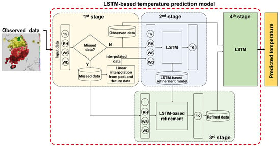
Figure 4 shows the architecture of the proposed LSTM-based temperature prediction model with a missing data refinement function incorporated. The proposed model is composed of four processing stages. The first stage detects whether or not any component of an input vector is missed, where each input vector is composed of 4-dimensional weather data (temperature, RH, wind speed, and wind direction). If one or more components are missed, then each missed component is linearly interpolated with past and future observed data. This process is done for all the training data.
Next, the second stage constructs an LSTM-based refinement model using all the training data, in which the missed data are already linearly interpolated. The LSTM-based refinement model is composed of one input layer, two LSTM layers, and one output layer, where 4-dimensional weather data are also used for an input vector, as shown in the second stage of Figure 4.
After training the LSTM-based refinement model, the third stage of the proposed model predicts temperature for the times when the temperature data, which were already detected in the first stage, are missing. By doing this, the missed temperature data are replaced with the predicted data; this process is referred to as a refinement function. The last stage of the proposed model is identical to that of the conventional LSTM model, as described in Section 2.3. The difference between the conventional LSTM model and the proposed one is in that in the proposed model, the missing data are refined through the refinement function and then are combined with the collected data without any missing components to train the LSTM.
3.3. Selection of Hyperparameters of LSTM
As weather is a chaotic process, many different factors play pivotal roles in controlling the change of a weather variable. Likewise, the deep structure of a neural network functions as very complex logic; thus, changing the network factors affects the prediction results. The network factors, called neural network hyperparameters, include the learning rate, batch size, number of epochs, regularization, weight initialization, number of hidden layers, number of nodes, etc. [24].
For hidden layers, activation functions determine whether the input feature is considered to be connected to the output nodes. In general, the activation functions need to be bounded. If the value of an activation function is above a certain bound, it is considered activated. If it is less than the bound, it is discarded. To make the proposed LSTM-based prediction model focus on weather data, especially temperature, we need to use several activation functions, such as linear, sigmoid, and ReLU functions. To this end, each of these three activation functions is employed in this model, and one of them is chosen for the best prediction accuracy. The ReLU was ultimately selected through this process and will be discussed in Section 4.3.
Similarly, the effect of different combinations of the numbers of LSTM layers and hidden nodes on the prediction accuracy is investigated by changing the LSTM layers from 2 to 6 and 192 to 480, with 96 hops for the hidden nodes. As a result, the number of LSTM layers is selected as 4, and the number of hidden nodes is selected as 384.
4. Experiments and Discussion
This section first briefly reviews a unified model (UM) that delivers the forecast results. Then, the database used in this paper is described. After that, the prediction accuracy of the proposed LSTM-based temperature prediction model is evaluated, where three LSTM models with the refinement function proposed in Section 3.2 are individually trained for hourly temperature predictions such as 6, 12, 24 h predictions. In addition, the other two LSTMs with the proposed refinement function are trained for 7 and 14 day temperature predictions. To compare the performance of the proposed model, the DNNs and conventional LSTMs in Section 2.1 and Section 2.3, respectively, are implemented for 6, 12, and 24 h temperature predictions, where missing data were simply ignored. Next, the conventional LSTMs were also implemented for 7 and 14 day temperature predictions, where two simple strategies for processing missing data, such as ignorance and linear interpolation, are applied. Finally, the prediction accuracy of the proposed model is compared with that of the UM model with the same weather data.
Note here that different LSTMs are evaluated using different values of the hyperparameters to examine the effectiveness of the hyperparameter set on the prediction accuracy, as described in Section 3.3. Therefore, throughout this paper, the numbers in the parentheses after LSTM, denoted as LSTM(x, y), mean that the number of LSTM layers is x, and the number of hidden nodes is y.
4.1. UM Model
The KMA has been conducting weather forecasts since 2010 based on the unified model (UM) developed by the U.K. Met Office [25]. The weather forecasting system of KMA consists of three NWP systems: Global Data Assimilation and Prediction System (GDAPS), Regional Data Assimilation and Prediction System (RDAPS), and Local Data Assimilation and Prediction System (LDAPS). The predictions of GDAPS and RDAPS are used as the boundary conditions for the operations of RDAPS and LDAPS, the domains of which are represented in Figure 5. As shown in the figure, RDPAS and LDAPS cover East Asia and South Korea with horizontal resolutions of 12 km × 12 km and 1.5 km × 1.5 km, respectively. Both systems have 70 sigma vertical layers, but the top heights are set to 80 km and 40 km for the RDAPS and LDAPS, respectively.
4.2. Database
In this study, we prepared the weather data released by the KMA, where the observations for all the observations including temperature, relative humidity, wind speed, and wind direction were made every hour [31]. The weather data were observed for around 37 years (from November 1981 to December 2017) from three different locations in South Korea (Seoul, Gyeonggi, and Jeolla), and these data were divided into two datasets: the data for around 36 years (from November 1981 to December 2016) were used as a training set, and the data for one year (from January 2017 to December 2017) as a test set. Note here that the period of weather data recording for the training set did not overlap that for the test data. Therefore, all the prediction models in this paper were trained and evaluated by using the training data and test data, respectively, unless there was no additional explanation for the training and test set. In addition, each prediction model per location was constructed, and the prediction accuracy for the model was averaged over three locations.
The performance was averaged over the three different prediction models. Moreover, some of the weather factors in the training set were missing, with 38%, 21%, 19%, and 11% missing data for relative humidity, wind speed, wind direction, and temperature, respectively. Since the number of missing data was relatively large, we developed a technique for dealing with the missed data, as described in Section 3.2. The performance comparison was done by calculating the RMSE and mean bias error (MBE) between the real observed temperature, and the predicted temperature, at a time, t, which are defined as
and
where N is the total number of times for the evaluation.
4.3. Comparison Between DNN and LSTM
In this subsection, we compare the prediction accuracy of the RMSE between the DNN model in Section 2.1 and the LSTM model in Section 2.3. Here, the architectures of the DNN and the LSTM model follow the previous works in [12,21], respectively. In particular, the numbers of LSTM layers and hidden nodes were set to 2 and 192, respectively. In both the DNN-based and LSTM-based temperature prediction models, the missing data were simply ignored for training and testing the models. In addition, each DNN or LSTM was implemented with three different activation functions: linear, sigmoid, and ReLU.
Table 3 compares RMSEs of DNN- and LSTM-based temperature prediction models according to different activation functions. It was shown from the table that LSTM(2,192) provided a lower RMSE than the DNN for all activation functions and three different time steps. In addition, the RMSEs of LSTM employing the ReLU activation function were smaller than those employing the linear and sigmoid activation functions for all three time-steps. Based on this experiment, the ReLU activation function was only considered for the following discussion, as mentioned in Section 3.3.
4.4. Comparison of LSTMs with Different Refinement Functions
Table 4 shows the performance comparison of LSTMs according to different missing data refinement functions for 6, 12, and 24 h temperature predictions. Here, the numbers of LSTM layers and hidden nodes were also set to 2 and 192, respectively, resulting in LSTM(2,192). However, instead of ignoring missing data, the linear interpolation refinement that interpolated the missing data with adjacent observed temperature data was incorporated into LSTM(2,192). As a result, it is shown in the table that LSTM(2,192) with linear interpolation greatly reduced the RMSE compared to the RMSE ignoring the missing data. Next, our proposed LSTM-based refinement function was applied to LSTM(2,192). Consequently, the LSTM(2,192) with LSTM-refinement further reduced the RMSE, especially for 12 and 24 h temperature predictions.
Next, in order to examine the effectiveness of the different hyperparameters on the performance of LSTM with the proposed LSTM-based refinement function, several evaluations on LSTM were conducted by changing both the number of LSTM layers from 2 to 6 and the number of hidden nodes from 192 to 480. In this experiment, the training dataset described in Section 4.2 was split into subsets: one is the data set for around 34 years from November 1981 to December 2014, denoted as the 34-dataset, and the other is for the two years of data from January 2015 to December 2016, denoted as the 2-dataset. Then, each LSTM was trained and evaluated using the 34-dataset and 2-dataset, respectively, to set the hyperparameters. Note that there was no overlap between the 2-dataset in this subsection and the test set described in Section 4.2.
Table 5 compares the RMSEs according to different numbers of LSTM layers and hidden nodes, where the proposed LSTM-based refinement function was applied for 24 h temperature prediction. As shown in the table, we achieved the lowest RMSE when the numbers of LSTM layers and hidden nodes were set to 4 and 384, respectively, with a smaller number of hyperparameters than LSTM(4,480) or LSTM(5,384). Based on these, the performances of LSTM(4,384) for different prediction time periods were compared.
4.5. Comparison of LSTMs for Short and Long Period Temperature Prediction
First, LSTM(4,384) was trained using three different refinement approaches: (1) the ignorance of missing data (i.e., without refinement), (2) linear interpolation, and (3) the proposed LSTM-based refinement function. Table 6 compares the average RMSEs and MBEs of the three LSTMs and the UM for 6, 12, and 24 h temperature prediction. As shown in the table, the LSTM-based prediction models with/without refinement functions gave a lower average RMSE and MBEs than the UM for all the different time steps. Moreover, similar to Table 4, the LSTM(4,384) with a refinement function, such as linear interpolation or LSTM refinement, reduced the RMSE compared to that without any refinement. In particular, the LSTM(4,384) with the proposed LSTM-based refinement function was better than that with linear interpolation. Note here that the prediction accuracies for 12 h temperature prediction was a little worse than those for 24 h prediction. This was because the input data to the LSTM were composed of the data observed at the current time and previous 11 h, while the target was advanced by 12 h, which might result in the day-night reversal due to the time difference between the input and target data of the models. This could be mitigated when the input data would be selected according to the target time.
Next, the proposed LSTM-based temperature prediction model was extended to predict 7 and 14 day future temperatures, and its RMSE was compared with the RMSEs by using the LSTM(4,384) without any refinement and with linear interpolation. As shown in Table 7, the tendency toward RMSE and MBE reduction for this long period temperature prediction was similar to that for 6, 12, and 24 h prediction. Interestingly, the proposed model with the LSTM-refinement had a 3.06 RMSE for 14 day prediction, which was lower than the DNN for 24 h predictions, as shown in the third row of Table 3. Moreover, the RMSE of the proposed LSMT-based model seems to be lower than that reported in [32], where a RMSE around 3 was achieved for 69–91 h (around 4 day) predictions and an RMSE of around 4 for 261–283 h (around 12 day) predictions.
4.6. Comparison with the UM Model
As mentioned above, in order to assess the potential usability of the proposed LSTM-based temperature prediction model, the accuracy comparison between the proposed model and LDAPS was conducted for 24 h temperature predictions from January 2017 to December 2017. In addition, the temperature predicted by the proposed model was compared with the forecast results of the UM model. It was confirmed that average RMSEs were 1.39, 1.45, and 1.52 for all 6, 12, and 24 h temperature predictions, respectively, as shown in the last row of Table 6. Note that unfortunately the KMA only provided up to a 48 h prediction of LDAPS; thus, we could not compare the performance for 7 and 14 day temperature predictions. Based on this experiment, which used one-year weather data, the proposed LSTM-based temperature prediction model achieved a lower RMSE for 24 h predictions than the UM model.
Figure 6 illustrates a time-series plot of the observed and predicted temperature data for two months (August to October 2017) in Seoul, Korea for 24-h (1-day) prediction. In the figure, four different models are compared, including the three models described in Table 6 and the UM LDAPS. As shown in the figure, the 24 h temperatures predicted by the proposed LSTM-based model employing the LSTM-refinement were, on average, close to those of the observed data. In particular, the proposed model had a lower average RMSE measured from August to October 2017 than LDAPS.
However, when the season changed, the proposed LSTM-based temperature prediction model was less accurate than that for the other periods. For example, we divided the 24 h prediction results of Figure 6 at weekly intervals, as shown in Figure 7, where each bar in the figure was drawn after averaging the RMSE over each week, and the vertical line at the top of each bar denotes the MBE of each RMSE. As shown in the figure, the week that contained the lowest temperature from the graph had a relatively higher RMSE than that of the other weeks. Nevertheless, it was shown that the proposed LSTM-based model still achieved better performance than LDAPS over the entire two month duration.
Finally, Figure 8 illustrates a time-series plot of the observed and predicted temperature data for two months (August to October 2017) in Seoul, Korea for 7 day and 14 day predictions. Note that only three different models in Table 7 were compared in this figure, because KMA only provided up to 48 h prediction result for LDAPS, as mentioned earlier. As shown in the figure, as the prediction period increased as 7 and 14 days, the prediction errors of the proposed LSTM-based temperature prediction model with LSTM-refinement were significantly smaller than those of other models, which implies that the LSTM-refinement contributed to providing a better fit to the pattern of the real observed data than linear interpolation. Similar to Figure 7 and Figure 9a,b show the averaged RMSEs and MBEs over each week for 7 day and 14 day temperature predictions shown in Figure 8a,b, respectively. It was clear that the proposed model achieved lower RMSEs than other LSTM-based prediction models for all the weeks.
5. Conclusions
In this paper, a neural network-based temperature prediction model has been proposed to keep track of temperature variations from 6 h to 14 day time periods through a consideration of the major influences of the primary weather variable. The proposed model was based on an LSTM neural network to fit the time-series data. In particular, the missing data, which frequently occur in the collected weather database, were refined by using an LSTM framework with temperature, relative humidity, wind speed, and wind direction. Then, the proposed LSTM-based model was implemented to predict temperature for short time periods such as 6, 12, and 24 h. In addition, it was also extended to predict temperature for relatively long time periods, such as 7 and 14 days. The performance evaluation used actual weather data for 37 years (from 1981 to 2017) at three different locations in South Korea, including hourly-based measurements for temperature, humidity, wind speed, and wind direction. In addition, the RMSE between observed and predicted temperatures was measured for each of the neural network models.
First, the effectiveness of the hyperparameters in the LSTM on prediction accuracy was examined. As a result, the number of LSTM layers and the number of hidden nodes were set to 4 and 384, respectively, for the proposed model. Next, the performance of the proposed model was evaluated and compared with that of the conventional LSTM-based and DNN-based models with either no refinement or linear interpolation refinement. Results showed that the proposed LSTM-based model gave the RMSE of 0.79 degrees Celsius for 24 h predictions while the conventional LSTM without any refinement and with linear interpolation had RMSEs of 1.02 and 0.84 degrees Celsius, respectively, and the UM model based on LDAPS provided by the Meteorological Office of South Korea achieved an RMSE of 1.52 degrees Celsius. In addition, the proposed LSTM-based model employing LSTM-refinement achieved RMSEs of 2.81 and 3.06 degrees Celsius for 7 and 14 day predictions, respectively, while the conventional LSTM-based model with linear interpolation provided RMSEs of 3.05 and 3.21 degrees Celsius for 7 and 14 day predictions, respectively.
However, the prediction accuracy of the proposed model needs to be improved during periods of seasonal changes, when sudden temperature changes occur. According to the 24 h temperature prediction from August 2017 to October 2017, the proposed LSTM-based model during September 2017 provided a slightly higher average RMSE than the average RMSE over one year, while the proposed LSTM-based model still had a lower average RMSE than LDAPS during September 2017. Since the improvement of the prediction accuracy in this period will have a great influence on the improvement of the overall temperature prediction model, we are considering extending our research to improve prediction accuracy during the season-changing period by, for example, using a new form of neural networks, which have an attention architecture for tracking transient data changes.
Moreover, weather data, such as relative humidity, wind speed, and wind direction, were used to refine the missing data in this paper. Although this paper shows the validity of the performance of the proposed model based on the result for temperature prediction, we indicate that this model is also applicable to not only temperature but also to other weather factors. However, as a future work, we are interested in constructing a deep learning model for predicting temperature by directly using more weather factors, including soil temperatures or aerosols. In other words, all the weather data available will be brought together as input features for a DNN, which will be both a temperature predictor and a missing data refiner.
Author Contributions
All authors discussed the contents of the manuscript. H.K.K. contributed to the research idea and the framework of this study; C.H.S. and J.H.K. helped with discussion; I.P. and H.S.K. equally performed the experiments with equal contribution as first authors; and J.L. assisted the experiments.
Funding
This research was supported by the National Strategic Project–Fine particle of the National Research Foundation of Korea (NRF) funded by the Ministry of Science and ICT (MSIT), the Ministry of Environment (ME), and the Ministry of Health and Welfare (MOHW) (NRF-2017M3D8A1092022), and it was also supported by a GIST Research Institute (GRI) grant funded by the GIST in 2019.
Conflicts of Interest
The authors declare no conflict of interest.
References
- Parry, M.; Canziani, O.; Palutikof, J.; van der Linden, P.; Hanson, C. Climate Change 2007: Impacts, Adaptation and Vulnerability. Available online: https://www.ipcc.ch/site/assets/uploads/2018/03/ar4_wg2_full_report.pdf (accessed on 30 October 2019).
- Schulte, P.A.; Bhattacharya, A.; Butler, C.R.; Chun, H.K.; Jacklitsch, B.; Jacobs, T.; Kiefer, M.; Lincoln, J.; Pendergrass, S.; Shire, J.; et al. Advancing the framework for considering the effects of climate change on worker safety and health. J. Occup. Environ. Hyg. 2016, 13, 847–865. [Google Scholar] [CrossRef] [PubMed]
- Abhishek, K.; Singh, M.P.; Ghosh, S.; Anand, A. Weather forecasting model using artificial neural network. Procedia Technol. 2012, 4, 311–318. [Google Scholar] [CrossRef]
- Campbell, S.D.; Diebold, F.X. Weather forecasting for weather derivatives. J. Am. Stat. Assoc. 2005, 100, 6–16. [Google Scholar] [CrossRef]
- De Giorgi, M.G.; Ficarella, A.; Tarantino, M. Assessment of the benefits of numerical weather predictions in wind power forecasting based on statistical methods. Energy 2011, 36, 3968–3978. [Google Scholar] [CrossRef]
- Zhao, T.; Guo, W.; Hu, C. Calibrating and evaluating reanalysis surface temperature error by topographic correction. J. Clim. 2008, 21, 1440–1446. [Google Scholar] [CrossRef]
- Sekula, P.; Bokwa, A.; Bochenek, B.; Zimnoch, M. Prediction of air temperature in the Polish Western Carpathian Mountains with the ALADIN-HIRLAM numerical weather prediction system. Atmosphere 2019, 10, 186. [Google Scholar] [CrossRef]
- Yi, J.; Prybutok, V.R. A neural network model forecasting for prediction of daily maximum ozone concentration in an industrialized urban area. Environ. Pollut. 1996, 92, 349–357. [Google Scholar] [CrossRef]
- Jiang, D.; Zhang, Y.; Hu, X.; Zeng, Y.; Tan, J.; Shao, D. Progress in developing an ANN model for air pollution index forecast. Atmos. Environ. 2004, 38, 7055–7064. [Google Scholar] [CrossRef]
- Ghielmi, L.; Eccel, E. Descriptive models and artificial neural networks for spring frost prediction in an agricultural mountain area. Comput. Electron. Agric. 2006, 54, 101–114. [Google Scholar] [CrossRef]
- Cao, Q.; Ewing, B.T.; Thompson, M.A. Forecasting wind speed with recurrent neural networks. Eur. J. Oper. Res. 2012, 221, 148–154. [Google Scholar] [CrossRef]
- Hossain, M.; Rekabdar, B.; Louis, S.J.; Dascalu, S. Forecasting the weather of Nevada: A deep learning approach. In Proceedings of the International Joint Conference on Neural Networks (IJCNN), Killarney, Ireland, 12–17 July 2015; pp. 1–6. [Google Scholar]
- Glorot, X.; Bordes, A.; Benjio, Y. Deep sparse rectifier neural networks. In Proceedings of the 14th International Conference on Artificial Intelligence and Statistics, Fort Lauderdale, FL, USA, 11–13 April 2011; pp. 315–323. [Google Scholar]
- Abadi, M.; Barham, P.; Chen, J.; Chen, Z.; Davis, A.; Dean, J.; Devin, M.; Ghemawat, S.; Irving, G.; Isard, M.; et al. TensorFlow: A system for large-scale machine learning. In Proceedings of the 12th USENIX Conference on Operating Systems Design and Implementation, Savannah, GA, USA, 2–4 November 2016; pp. 265–283. [Google Scholar]
- Glorot, X.; Benjio, Y. Understanding the difficulty of training deep feedforward neural networks. In Proceedings of the 13th International Conference on Artificial Intelligence and Statistics, Sardinia, Italy, 13–15 May 2010; pp. 249–256. [Google Scholar]
- Rumelhart, D.E.; Hinton, G.E.; Williams, R.J. Learning representations by back-propagating errors. Nature 1986, 323, 533–536. [Google Scholar] [CrossRef]
- Kingma, D.P.; Ba, J.L. ADAM: A method for stochastic optimization. In Proceedings of the 3rd International Conference on Learning Representations, San Diego, CA, USA, 7–9 May 2015; pp. 1–15. [Google Scholar]
- Graves, A.; Jaitly, N.; Mohamed, A. Hybrid speech recognition with deep bidirectional LSTM. In Proceedings of the IEEE Workshop on Automatic Speech Recognition and Understanding (ASRU), Olomouc, Czech Republic, 8–12 December 2013; pp. 273–278. [Google Scholar]
- Hochreiter, S. The vanishing gradient problem during learning recurrent neural nets and problem solutions. Int. J. Uncertain. 1998, 6, 107–116. [Google Scholar] [CrossRef]
- Chung, J.; Gulcehre, C.; Cho, K.; Bengio, Y. Empirical evaluation of gated recurrent neural networks on sequence modeling. arXiv 2014, arXiv:1412.3555. [Google Scholar]
- Greff, K.; Srivastava, R.K.; Koutnik, J.; Steunebrink, B.R.; Schmidhuber, J. LSTM: A search space odyssey. IEEE Trans. Neural Netw. Learn. Syst. 2017, 28, 2222–2232. [Google Scholar] [CrossRef] [PubMed]
- Sundermeyer, M.; Schlüter, R.; Ney, H. LSTM neural networks for language modeling. In Proceedings of the Annual Conference of the International Speech Communication Association (Interspeech), Portland, OR, USA, 9–13 September 2012; pp. 194–197. [Google Scholar]
- Korea Meteorological Office of Weather Online Resources. Synoptic Weather Observation Data. Available online: https://web.kma.go.kr/eng/biz/forecast_02.jsp (accessed on 29 October 2019).
- Deep Learning for Java. Available online: https://deeplearning4j.org/tutorials/11-hyperparameter-optimization (accessed on 18 May 2019).
- Met Office Weather Forecasts for the UK. Available online: https://www.metoffice.gov.uk/research/approach/modelling-systems/unified-model/index (accessed on 29 October 2019).
- Wilson, D.R.; Ballard, S.P. A microphysically based precipitation scheme for the UK meteorological office unified model. Q. J. R. Meteor. Soc. 1999, 125, 1607–1636. [Google Scholar] [CrossRef]
- Gregory, D.; Rowntree, P.R. A mass flux convection scheme with representation of cloud ensemble characteristics and stability-dependent closure. Mon. Weather Rev. 1990, 118, 1483–1506. [Google Scholar] [CrossRef]
- Essery, R.; Best, M.; Cox, P. MOSES 2.2 Technical Documentation. Available online: http://jules.jchmr.org/sites/default/files/HCTN_30.pdf (accessed on 12 October 2019).
- Lock, A.P.; Brown, A.R.; Bush, M.R.; Martin, G.M.; Smith, R.N.B. A new boundary layer mixing scheme. Part I: Scheme description and single-column model tests. Mon. Weather Rev. 2000, 128, 3187–3199. [Google Scholar] [CrossRef]
- Edwards, J.M.; Slingo, A. Studies with a flexible new radiation code: 1. Choosing a configuration for a large-scale model. Q. J. R. Meteorol. Soc. 1996, 122, 689–719. [Google Scholar] [CrossRef]
- Korea Meteorological Administration. Surface Observation. Available online: https://web.kma.go.kr/eng/biz/observation_02.jsp (accessed on 30 October 2019).
- Jeong, J.; Lee, S.-J. A statistical parameter correlation technique for WRF medium-range prediction for near-surface temperature and wind speed using generalized linear model. Atmosphere 2018, 9, 291. [Google Scholar] [CrossRef] [Green Version]
Figure 1.
An example of (a) a deep neural network (DNN) composed of an input layer, hidden layers, and an output layer and (b) three different DNNs with different numbers of input nodes.
Figure 1.
An example of (a) a deep neural network (DNN) composed of an input layer, hidden layers, and an output layer and (b) three different DNNs with different numbers of input nodes.

Figure 2.
An example of a simple recurrent neural network (RNN).

Figure 3.
(a) A Long Short-Term Memory (LSTM) memory block with an input, a forget, and an output gate, and (b) the architecture of a conventional LSTM neural network with a T-dimensional input vector and L hidden nodes.
Figure 3.
(a) A Long Short-Term Memory (LSTM) memory block with an input, a forget, and an output gate, and (b) the architecture of a conventional LSTM neural network with a T-dimensional input vector and L hidden nodes.

Figure 4.
Architecture of the proposed LSTM-based temperature prediction model with a missing data refinement function incorporated.
Figure 4.
Architecture of the proposed LSTM-based temperature prediction model with a missing data refinement function incorporated.

Figure 5.
Domain of the UM system, where Regional Data Assimilation and Prediction System (RDAPS) and Local Data Assimilation and Prediction System (LDAPS) are denoted by blue and red lines [23].
Figure 5.
Domain of the UM system, where Regional Data Assimilation and Prediction System (RDAPS) and Local Data Assimilation and Prediction System (LDAPS) are denoted by blue and red lines [23].

Figure 6.
Daily basis plot of the observed and predicted temperature data for two months from August to October in Seoul, Korea for 24 h (1 day) prediction.
Figure 6.
Daily basis plot of the observed and predicted temperature data for two months from August to October in Seoul, Korea for 24 h (1 day) prediction.

Figure 7.
Weekly RMSE and MBE of the proposed LSTM-based model with LSTM-refinement and the UM LDAPS for two months from August to October in Seoul, Korea for 24 h (1 day) temperature prediction.
Figure 7.
Weekly RMSE and MBE of the proposed LSTM-based model with LSTM-refinement and the UM LDAPS for two months from August to October in Seoul, Korea for 24 h (1 day) temperature prediction.

Figure 8.
Daily plot of the observed and predicted temperature data for two months from August to October in Seoul, Korea for (a) 7 day and (b) 14 day prediction.
Figure 8.
Daily plot of the observed and predicted temperature data for two months from August to October in Seoul, Korea for (a) 7 day and (b) 14 day prediction.

Figure 9.
Weekly RMSE and MBE of the LSTM-based models with different refinement methods for two months from August to October in Seoul, Korea for (a) 7 day and (b) 14 day temperature prediction.
Figure 9.
Weekly RMSE and MBE of the LSTM-based models with different refinement methods for two months from August to October in Seoul, Korea for (a) 7 day and (b) 14 day temperature prediction.


Table 1.
Comparison of correlation coefficients between temperature and other weather factors.
| Weather Factors | Wind Direction | Wind Speed | Relative Humidity | Cumulative Precipitation | Vapor Pressure | Barometric Pressure |
|---|---|---|---|---|---|---|
| Correlation | 0.71 | 0.69 | 0.64 | 0.38 | 0.25 | 0.30 |
Table 2.
Physical options of unified model (UM)-based numerical weather prediction (NWP) system used in KMA.
Table 2.
Physical options of unified model (UM)-based numerical weather prediction (NWP) system used in KMA.
| Physical Options | Scheme |
|---|---|
| Microphysics | Mixed-phase precipitation [26] |
| Cumulus scheme | Mass flux convection with convective available potential energy (CAPE) closure [27] |
| Land surface model scheme | Met office surface exchange scheme (MOSES)-II land-surface [28] |
| Planetary boundary layer (PBL) scheme | First-order non-local boundary layer scheme [29] |
| Radiation scheme | Edwards-Slingo general 2-stream scheme [30] |
Table 3.
Performance comparison of the root-mean-squared error (RMSE) according to different activation functions applied to the DNN and conventional LSTM.
Table 3.
Performance comparison of the root-mean-squared error (RMSE) according to different activation functions applied to the DNN and conventional LSTM.
| Model | Activation Function | Hour | Average | ||
|---|---|---|---|---|---|
| 6 | 12 | 24 | |||
| DNN | linear | 1.86 | 2.81 | 3.77 | 2.81 |
| sigmoid | 1.74 | 2.67 | 3.52 | 2.67 | |
| ReLU | 1.59 | 2.49 | 3.11 | 2.40 | |
| Conventional LSTM(2,192) | linear | 1.21 | 1.47 | 1.33 | 1.34 |
| sigmoid | 1.19 | 1.31 | 1.15 | 1.21 | |
| ReLU | 1.12 | 1.29 | 1.13 | 1.18 | |
Table 4.
Performance comparison of the RMSE of the LSTMs with the linear interpolation and LSTM-refinement for 6, 12, and 24 h temperature predictions.
Table 4.
Performance comparison of the RMSE of the LSTMs with the linear interpolation and LSTM-refinement for 6, 12, and 24 h temperature predictions.
| Hour | 6 | 12 | 24 | |
|---|---|---|---|---|
| Model | ||||
| Conventional LSTM(2,192) from Table 3 | 1.12 | 1.29 | 1.13 | |
| LSTM(2,192)—linear interpolation | 0.77 | 1.24 | 1.02 | |
| LSTM(2,192)—LSTM-refinement | 0.77 | 1.20 | 1.01 | |
Table 5.
Performance comparison of the RMSE of LSTMs for 24 h temperature prediction according to different numbers of LSTM layers and hidden nodes, where the proposed LSTM-based refinement function was applied (Training data: November 1981 to December 2014, Test data: January 2015 to December 2016).
| No. of Hidden Nodes | 192 | 288 | 384 | 480 | |
|---|---|---|---|---|---|
| No. of LSTM Layers | |||||
| 2 | 1.19 | 1.16 | 0.94 | 0.89 | |
| 3 | 0.99 | 0.89 | 0.86 | 0.88 | |
| 4 | 0.94 | 0.86 | 0.82 | 0.95 | |
| 5 | 0.87 | 0.86 | 0.84 | 0.88 | |
| 6 | 0.98 | 0.93 | 0.89 | 0.87 | |
Table 6.
Performance comparison of the RMSE and MBE of the LSTMs with the linear interpolation and LSTM-refinement, as well as the UM model for 6, 12, and 24 h temperature prediction.
Table 6.
Performance comparison of the RMSE and MBE of the LSTMs with the linear interpolation and LSTM-refinement, as well as the UM model for 6, 12, and 24 h temperature prediction.
| Hour | RMSE | MBE | |||||
|---|---|---|---|---|---|---|---|
| Model | 6 | 12 | 24 | 6 | 12 | 24 | |
| LSTM(4,384)–without refinement | 1.08 | 1.14 | 1.02 | −0.05 | 0.09 | 0.15 | |
| LSTM(4,384)–linear interpolation | 0.64 | 1.04 | 0.84 | 0.02 | −0.06 | 0.08 | |
| LSTM(4,384)–LSTM-refinement | 0.53 | 1.01 | 0.79 | −0.01 | 0.05 | 0.04 | |
| UM (LDAPS) | 1.39 | 1.45 | 1.52 | −0.37 | −1.18 | 1.76 | |
Table 7.
Performance comparison of the RMSE and MBE of the LSTMs with linear interpolation and LSTM-refinement for 7 and 14 day temperature predictions.
Table 7.
Performance comparison of the RMSE and MBE of the LSTMs with linear interpolation and LSTM-refinement for 7 and 14 day temperature predictions.
| Day | RMSE | MBE | |||
|---|---|---|---|---|---|
| Model | 7 | 12 | 7 | 12 | |
| LSTM(4,384)–without refinement | 3.15 | 3.61 | −2.08 | −3.26 | |
| LSTM(4,384)–linear interpolation | 3.05 | 3.21 | 0.93 | 1.68 | |
| LSTM(4,384)–LSTM-refinement | 2.81 | 3.06 | 0.41 | −0.79 | |
© 2019 by the authors. Licensee MDPI, Basel, Switzerland. This article is an open access article distributed under the terms and conditions of the Creative Commons Attribution (CC BY) license (http://creativecommons.org/licenses/by/4.0/).
Share and Cite
MDPI and ACS Style
Park, I.; Kim, H.S.; Lee, J.; Kim, J.H.; Song, C.H.; Kim, H.K. Temperature Prediction Using the Missing Data Refinement Model Based on a Long Short-Term Memory Neural Network. Atmosphere 2019, 10, 718. https://doi.org/10.3390/atmos10110718
AMA Style
Park I, Kim HS, Lee J, Kim JH, Song CH, Kim HK. Temperature Prediction Using the Missing Data Refinement Model Based on a Long Short-Term Memory Neural Network. Atmosphere. 2019; 10(11):718. https://doi.org/10.3390/atmos10110718
Chicago/Turabian StylePark, Inyoung, Hyun Soo Kim, Jiwon Lee, Joon Ha Kim, Chul Han Song, and Hong Kook Kim. 2019. "Temperature Prediction Using the Missing Data Refinement Model Based on a Long Short-Term Memory Neural Network" Atmosphere 10, no. 11: 718. https://doi.org/10.3390/atmos10110718
Note that from the first issue of 2016, this journal uses article numbers instead of page numbers. See further details here.