On the Use of Original and Bias-Corrected Climate Simulations in Regional-Scale Hydrological Scenarios in the Mediterranean Basin

Abstract

The response of Mediterranean small catchments hydrology to climate change is still relatively unexplored. Regional Climate Models (RCMs) are an established tool for evaluating the expected climate change impact on hydrology. Due to the relatively low resolution and systematic errors, RCM outputs are routinely and statistically post-processed before being used in impact studies. Nevertheless, these techniques can impact the original simulated trends and then impact model results. In this work, we characterize future changes of a small Apennines (Central Italy) catchment hydrology, according to two radiative forcing scenarios (Representative Concentration Pathways, RCPs, 4.5 and 8.5). We also investigate the impact of a widely used bias correction technique, the empirical Quantile Mapping (QM) on the original Climate Change Signal (CCS), and the subsequent alteration of the original Hydrological Change Signal (HCS). Original and bias-corrected simulations of five RCMs from Euro-CORDEX are used to drive the CETEMPS hydrological model CHyM. HCS is assessed by using monthly mean discharge and a hydrological-stress index. HCS shows a large spatial and seasonal variability where the summer results are affected by the largest decrease of mean discharge (down to −50%). QM produces a small alteration of the original CCS, which generates a generally wetter HCS, especially during the spring season.

1. Introduction

Projecting the response of the hydrological cycle to climate change is essential for managing freshwater resources in future decades. An accurate representation of hydrological regime changes, according to different greenhouse gases (GHGs) concentration scenarios, is one of the most challenging issues in climate change science. While representing a second-order effect of a temperature increase, precipitation change projections are affected by higher uncertainty. There is a particular concern on how different precipitation statistics (i.e., mean and extremes) will scale with different levels of global warming [1,2]. In spite of these uncertainties, a large consensus prevails on expecting an acceleration of the hydrological cycle in warmer climate conditions [3,4,5,6,7,8,9]. Another level of complexity is added when projected changes, to be efficiently informative, have to be scaled at the regional scale and tailored in a function of peculiar regional features. This represents a particularly urgent need for regions, which are responding to climate change faster than the world average such as for the Mediterranean basin [10,11,12]. While the response of large basin hydrology to climate change has been tackled by several studies [13,14,15,16,17,18,19], the response of small catchments hydrology is still relatively unexplored. Furthermore, these latter systems are implicitly more responsive to precipitation regime alterations and, consequently, highly vulnerable to climate extremes (both droughts and floods). Such a reduced climate change resilience requires accurate climate information, which is aimed at enabling stakeholders to limit current and future climate effects. Regional Climate Model (RCM) simulations are established tools for climate impact studies [20,21,22]. However, due to imperfections on physical processes formulation and parameterizations, coupled with the unpredictability of future natural variability, RCMs are still affected by systematic errors that can result in unrealistic results of the impact models’ results [23,24,25]. In addition, when future climate information is sought at a regional scale to a local scale, climate simulations are affected by the representativeness error, which does not arise from incorrect physical formulation, but rather from the simulated and observed fields’ spatial scale mismatch [26]. Generally, the combination of these errors leads to substantial differences in climate simulations and observations of statistical properties. For these reasons, in recent years, climate simulations’ bias adjustment has become a routine procedure to properly connect climate simulations to impact studies [24]. However, even though the post-processing techniques produce simulations’ statistical properties close to the observed climate, they can potentially modify original simulations of the Climate Change Signal (CCS, i.e., difference/ratio between climate statistics of a future and a historical temporal segment). The modification of the original CCS implicitly alters the results of impact models [27,28,29,30,31,32,33,34,35]. The plausibility of letting bias correction alter the original simulated CCS is currently strongly debated. The aspect conferring plausibility to CCS alteration, produced by a statistical post-processing phase, is the assumption of temporal stationary of climate model biases. This assumption is not universally recognized [33,36]. In the case of temporal-dependency of model biases, a CCS alteration should be avoided because of mathematical artifacts [33]. In recent years, this assumption has been investigated through a pseudo-reality experiment [37,38], which allowed for different interpretations [33,34]. On the other hand, several studies [23,24,31,34] point out that biased climate model simulations produce biased CCS and they found a dependence between biases and the magnitude of the simulated values (i.e., higher precipitation affected by larger bias) such as an intensity-dependence of the model biases. Intensity-dependence model biases refer to the fact that the higher the simulated value is, the higher the bias magnitude affecting such a value would be. In this context, the summer season values and related CCS could be more largely affected by biases [23]. According to this perspective, the impact of bias correction on the original CCS would be beneficial as derived by the original simulations’ bias removal. In any case, accepting the need for some climate model outputs statistical adjustment, its formulation and the potential artifacts introduced must be carefully evaluated in the entire modeling chain (climate model and impact model simulations). It is essential to avoid a “blind” usage of such techniques over the wide spectrum of climate impact applications [39,40]. In this regard, this study provides empirical evidence on the impact of using original and bias corrected climate simulations on defining basin-scale hydrological future changes, under two different emission scenarios. Specifically, we will discuss the alteration of the CCS and its propagation in the Hydrological Change Signal (HCS) through the use of an ensemble of five RCMs, according to the Representative Concentration Pathways 4.5 and 8.5 [41,42,43]. Different works attempt to analyze the impact of CCS on the flood hazard in Europe [44,45,46,47,48], where the importance of investigating the potential effect of a warmer atmosphere on hydrological extremes at regional scales is highlighted. To this aim, original and bias-corrected climate simulations will be used as forcing fields for the CETEMPS Hydrological Model (CHyM) operationally used for hydrological risk forecast over Italy. Similar to the CCS, the HCS will be derived by comparing future and reference periods among hydrological simulations. This comparison refers to both mean and extreme discharge flows. The latter will be derived by means of the computation of a hydrological stress conditions index. Regarding what concerns the statistical bias correction, it consists of a widely employed technique in climate services such as empirical Quantile Mapping (QM). Its central idea is to establish a correction function (CF) that maps a simulated climate distribution on a corresponding observation-based reference distribution during a calibration period and then it applies the CF to the entire simulation. In this study, we use a QM application, which implicitly couples bias correction and downscaling properties. In fact, we derived the QM correction functions considering observed products at a station scale. This application implicitly takes into account systematic biases and the representativeness error arising from the spatial-scale gap between simulations and observations such as in References [26,34,35,49,50,51]. We take advantage of five high-resolution (~12 km) climate simulations provided by the Euro-CORDEX initiative [52]. Climate simulations are extracted from the nearest grid nodes to reference observational sites within the Pescara-Aterno river basin (Central Italy) that represents the study area. Original and bias corrected climate simulations, according to the two emission scenarios, have been, in turn, used as forcing fields for the hydrological simulations of a reference and future period. Each acronym found throughout the manuscript are defined and reported in the Appendix A.

2. Study Area, Materials, Methods, and Analyses

Data collection was carried out in the eastward section of the Aterno-Pescara river catchment area (Figure 1), which is the largest and most inhabited watershed of the Abruzzo Region located in Central Italy. It comes with the longest river (about 145 km), which flows into the Adriatic Sea. The Aterno river originates from the northern part of the Abruzzo Region in the Laga Mountains area, on the western side of the Gran Sasso d’Italia major peak. Its course is parallel to the Apennines’ ridge for about 100 km in the south-east direction, before turning northeastward and becoming the “Aterno-Pescara” river. The Aterno part of the watershed is characterized by a torrential regime with significant infiltration. The substrate is mainly composed of calcareous and marly-calcareous terrain. The Pescara branch is connected to other tributaries and, from this point, the shallow runoff increases and the response to the precipitation becomes more rapid, for the presence of more frequent clayish sediments. The maximum discharge, on average, estimated at S. Teresa station (6 km upstream of the river outlet) is 594.08 m3/s, while the minimum discharge average is 18.40 m2/s (Aterno-Pescara Protection Program, Legislative Decree no. 152/2006).

2.1. Observed Data Sets

This study considers two climatic variables: 3-hourly mean temperature and 3-hourly cumulative precipitation. For each variable, observed and simulated time series refer to 17 reference sites chosen for properly taking into account the main climate and morphological sectors of the basin (coastal, hill, and mountain). The observed time series, which refer to the 2002-2016 period, are provided by the Abruzzo Regional Hydrological Service (

Table 1. Reference sites with weather stations providing data for the 2002–2016 period. Elevation data refer to both observational sites and the relative nearest grid node of the RCA4 RCM.

Station Name	Longitude (dec.)	Latitude (dec.)	Elevation (m a.s.l.)	Elevation RCA4 Nearest Grid Node (m a.s.l.)
Giulianova	13.9572	42.7513	68	171
Pescara	14.2205	42.4600	29	145
S. Teresa	14.1625	42.4213	12	114
Chieti	14.1672	42.3488	293	195
S. Stefano	13.6002	42.6505	820	868
Teramo	13.6772	42.6138	630	359
Arsita	13.7925	42.4805	470	988
Catignano	13.9455	42.3461	330	569
Caramanico	14.0191	42.1008	820	1126
Passo Lanciano	14.1091	42.1947	1306	786
Montereale	13.2444	42.5222	910	1120
Campotosto	13.4063	42.5361	1340	1300
Assergi	13.5105	42.4186	991	1410
L’Aquila	13.4316	42.3391	590	956
Barisciano	13.5830	42.3250	960	1160
Goriano Sicoli	13.7927	42.0933	969	760
Sulmona	13.9513	42.0580	370	843

).

The reasons for choosing station-scale observed data instead of widely used gridded observational data sets in climate services, e.g., ECAD-EOBS [53], are the following.

First, the latter results from an interpolation process. Its reliability relies on the density of observational stations, which is very poor in the study area [53,54,55].

Second, when considering high temporal (i.e., sub-daily) and spatial simulations (i.e., 12 km), gridded observational products offer daily temporal resolution and spatial resolution ~25 km (at the time this work is being written) in the studied area. This would involve an “upscaling” of the original simulations [56].

However, it must be considered that point-scale observations present limitations due to the small size of the time series (i.e., 15 years) available, which limits the calibration process of the bias correction functions.

2.2. Simulations

The simulated climate variables are extracted at the reference sites from the nearest grid nodes (Figure 2). Climate simulations are provided by five RCM runs in the context of the Euro-CORDEX initiative.

As can be seen in

Table 2. RCMs used in this study. All the RCMs share the same horizontal resolution of ~12.5 km and are forced by the RCPs 4.5 and 8.5.

RCM	Driving GCM (RCP 4.5 | RCP 8.5)
SMHI-RCA4	CERFACS-CNRM-CM5 ICHEC-EC-EARTH IPSL-CM5A-MR MOHC-HadGEM2-ES MPI-ESM-LR

, we consider simulations from the same RCM (RCA4), driven by five different Global Climate Models (GCMs). These simulations are chosen because they are the only ones archived at a 3-h temporal frequency as required to force the ChyM hydrological runs. For the simulations, we considered two 15-year segments, a future period (2081–2095), and a reference one (2002–2016). This choice of the reference period was imposed by the 3-hourly observed time series availability (2002–2016). In order to define the QM correction functions simulated and the observed reference (or calibration), the analyzed period must be the same.

2.3. The Hydrological Model Cetemps Hydrological Model (CHyM)

The Cetemps HYdrological Model (CHyM) is a distributed, grid-based model developed at the Centre of Excellence CETEMPS since 2002 for flood events’ early warning [57,58]. Nevertheless, the CHyM model has also been successfully used within the ACQWA project (www.acqwa.ch) to assess the climatic impact over the upper Po basin hydrological regime [16].

The model simulates the standard hydrological processes, such as surface runoff, infiltration, evapotranspiration, percolation, melting, and return flow. A comprehensive description of the physical processes, governing equations, and CHyM calculation schemes and parameterizations can be found in Reference [59]. In particular, evapotranspiration is computed according to Reference [60], where potential evapotranspiration is considered as a function of the evapotranspiration in soil saturation conditions. The actual evapotranspiration is a fraction of potential evapotranspiration and it is calculated as a linear function of ground relative humidity.

One of the main features of the model is the use of the Cellular Automata (CA) theory-based algorithms [61] to extract the drainage network starting from an arbitrary Digital Elevation Model (DEM) resolution for the spatialization of the rainfall and temperature fields by assimilating different data sources. The first algorithm defines the flow direction at every point on the DEM where singular points are present (pits or flat areas). A second algorithm is a CA-based numerical technique for assimilating different data sources of rainfall to rebuild the rainfall field on a grid. CA algorithms have been implemented and tested on a large number of different domains [58,59,62]. Results show a coherent reproduction of the meteorological data in gridded maps, starting from a sparse data set without any geometrical artifacts that often produce unrealistic rain gradients [59]. Extreme discharge values are usually defined through statistical-based thresholds, identified by means of percentiles and return periods. In order to guarantee reliable hydrological data, those methods require consistent historical discharge time series as well as quality ex-post control and application of filtering techniques.

For climatological applications, the CHyM model has been calibrated in the upper Po basin [16], which represents the Italian catchment where the longest historical discharge timeseries is available, as well as information about uncertainties associated with the application of the rating curve method [63]. As assessed by the same authors, the Po river dynamics can be considered representative of the conditions of many alluvial rivers in Europe and the same calibrated parameters have been used to set up hydrological simulations in this work. As for flood event detection, we introduced a discharge-based hydrological stress index, since the use of hydrological indices is very common in operational hydrology activities [64,65,66]. The Aterno-Pescara catchment is well instrumented with hydrometers, but rating curves, as well as river sections, are not available after 2005. For this reason, we decided to identify flood events as we do in operational applications, by means of a hydrological stress index, which has been calibrated over the Abruzzo Region in collaboration with the Civil Protection Functional Centre, in the framework of a specific agreement with CETEMPS (officially appointed as Civil Protection competence centre). Hydrological stress index thresholds were calibrated and validated upon hydrometric level thresholds, and used to predict flood events, as described in References [67,68].

The BDD (Best Discharge-Based Drainage) index is calculated for each grid-point of the drainage network, according to the following formula.

$$BDD{\left(t\right)}_{\mathrm{i},\mathrm{j}}=\frac{Q{\left(t\right)}_{\mathrm{i},\mathrm{j}}}{R_{\mathrm{i},\mathrm{j}}^2}$$

(1)

where Q and R represents the natural discharge and the hydraulic radius, respectively, associated with the grid point i-j at each hourly time step t. Index dimensions are expressed as mm/h. As for many other models (for a general reference, see Reference [69]), the hydraulic radius can be approximated as a linear function of the drained area.

Two warning BDD thresholds (orange and red thresholds) are then defined through a calibration/validation activity, carried out in collaboration with the Abruzzo Region Functional Centre (CFA), in the framework of the official agreement that ratifies CETEMPS as the official Centre of Competence for the regional Civil Protection. The BDD index is operationally used for the daily flood forecast over Italy. Its warning-level thresholds (reported in color-codes maps) are assessed in order to replicate the hydrometric level-based warningstates [70].

Since the BDD index calculation is given by the relationship between the natural discharge and the river geometry, which is represented by the hydrometric radius, the defined thresholds are found to be applicable for the whole drainage network.

2.4. Methods and Statistical Bias Correction of the Climate Simulations

In this study, we applied an empirical QM configuration, which is a statistical bias correction technique widely employed in climate services [33]. This method derives a quantile-specific correction function (CF) derived from the difference between the observed and simulated inverse Empirical Cumulative Distribution Functions (ecdfs, or quantile functions) during the calibration period. Considering the point-scale observed product, this QM configuration implicitly combines bias correction and downscaling properties.

The CF is determined for a set of physical values corresponding to discrete quantiles (1, 2, 3, …, 99) and then interpolated to adjust all the physical values (not only those corresponding to the quantiles where the function has been derived). In this case, it is used in a 3-hourly configuration of a purely empirical approach as in References [27,35,49,50,71,72,73], where a daily-based QM configuration was used.

Three main modifications to the standard QM configuration are applied in this study.

(i) CF Moving window. CF was built on a 91-day sliding time window centered on each day of the year. Given the 3-hourly QM configuration, for each time window iteration, an ecdf is built on a number of values corresponding to the size of the window (i.e., 91 days) times the number of the time steps in one day (i.e., 8), namely on 728 values. This latter value is then multiplied for the number of years constituting the period subjected to the correction (i.e., 728 × 15 = 10,920). The time window was set wide enough to adequately take into account weather patterns and extremes characterizing multi-month seasons [32]. In this way, the CF specifically adjusts for each 3-hourly time step of years within the period subjected to the statistical adjustment. The moving window prevents correction factor jumps that may occur when each month is statistically adjusted, according to its own CF.

Specific quantile-based correction factors are then applied to the physical values of the simulated time series under correction while obtaining a new statistically adjusted time series.

(ii) CF extrapolation is applied for the correction of a future period. The CF was constantly extrapolated beyond the highest and the lowest quantiles of the calibration period.

(iii) Preliminary adjustment of the simulation dry-day frequency, given the well-known overestimation of the very low precipitation events frequency produced by original RCMs [74,75], a correction is preliminarily performed on the dry 3-hourly time step for precipitation such as in Reference [35]. This consists of deriving the threshold beneath the simulated precipitation, which is considered equal to zero.

In this way, the CFs have been derived and applied only to the rainy 3-hourly time steps.

The 3-hourly rainfall and temperature field, simulated by each model set-up listed in Table 2, have been used as input to carry out the CHyM hydrological simulations for both future and reference periods. Each 15-years hydrological simulation is continuous and performed at an hourly time-step where the RCM’s output temporal resolution is set to 3 h. The hourly temperature has been obtained when considering the temperature value constant for the three consecutive hours. The cumulated 3-h precipitation amount has been divided by three as well.

2.5. Analyses

In this study, the analyses are applied to climate and hydrological fields as follows.

(i) Assessment of the CHyM driving fields, in terms of capability of the original and bias-corrected climate simulations (precipitation and temperature) to reproduce the observed station-scale statistical distributions during the reference period. In this context, biases are reported as the difference (°C) between simulation and observation for the temperature and, in relative terms, for the precipitation (i.e., (simulated statistics/observed statistics)-1). The impact of QM on the original temperature and precipitation CCS will be discussed as well. The CCS is derived as the difference between the future (2081–2095) and the reference (2002–2016) period statistics for the temperature, and, in terms of the relative ratio ((future statistics/reference statistics)-1), for the precipitation.

(ii) Assessment of the monthly mean discharge flow at Pescara river mouth simulated by CHyM forced by original and bias-corrected simulations during the reference period (2002–2016). In this context, an observation-driven CHyM simulation will be considered as a reference product. The impact of the bias correction on the hydrological scenarios will be investigated in terms of discharge variations (i.e., differences) between values characterizing a future period (2081–2095) and the reference period (2002–2016). This consists of the comparison of the HCS obtained with CHyM forced by original and bias-corrected climate simulations. The analyses will be focused on the point-scale HCS, considering the monthly mean discharge at the Pescara river mouth grid node. Furthermore, the spatial distribution of the mean discharge change will be presented over the whole Aterno-Pescara basin.

Lastly, expected changes regarding hydrological-stress conditions will be assessed. These latter conditions are identified by means of a dedicate index known as the Best Discharge-based Drainage (BDD, mm/h), which is aimed at detecting catchment segments that are most likely to be stressed by critical swelling discharge. Changes of the BDD index are represented by the number of events (i.e., number of hours) on which the BDD index value exceeds a predefined empirical threshold, specifically calibrated for the Aterno-Pescara basin.

3. Results and Discussions

3.1. Original and Bias Corrected Climate Simulations, Calibration Period, and Climate Change Signal

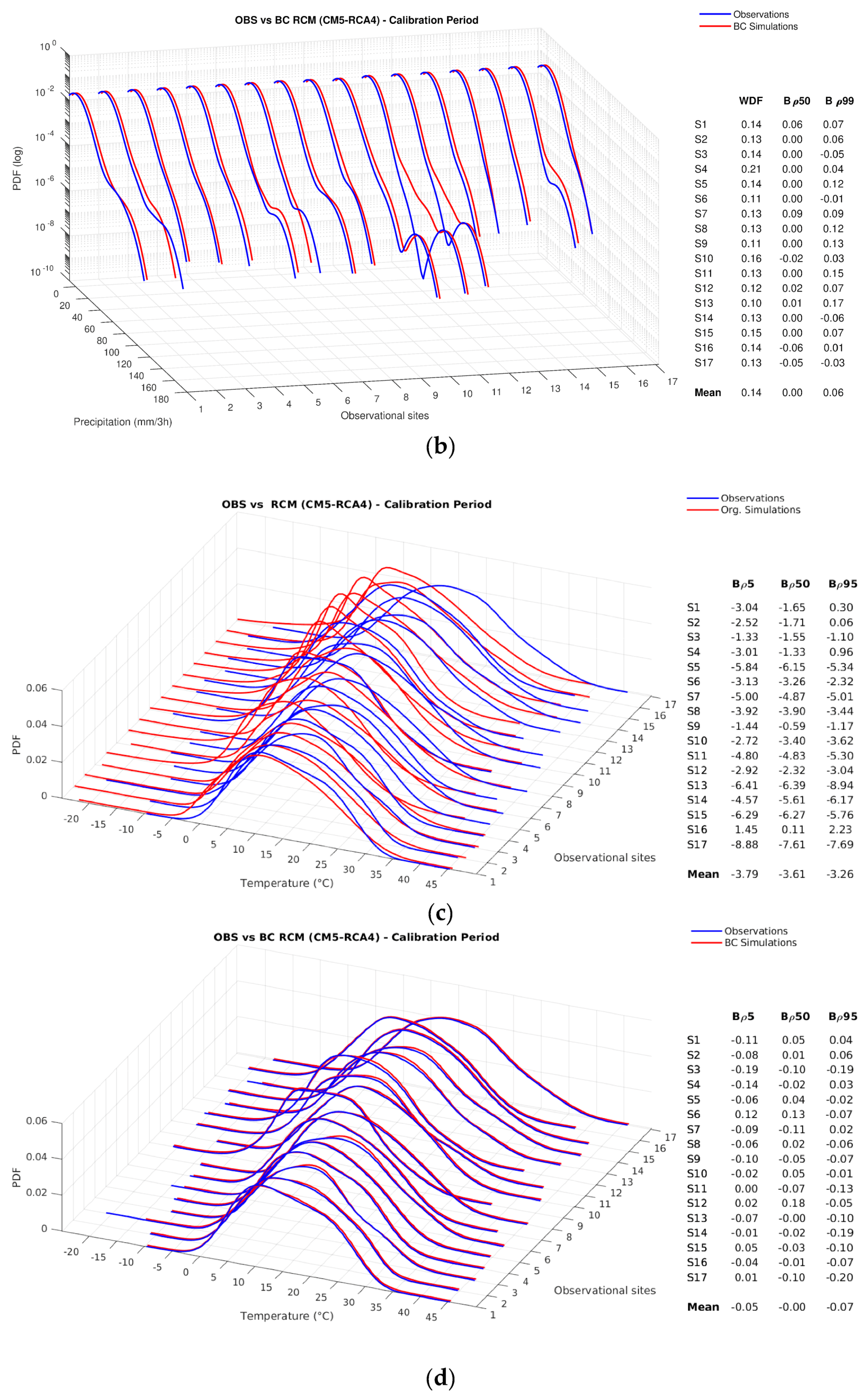
3.1.1. Calibration Period

In this section, we will start providing an analysis of the original and bias-corrected climate simulation Probability Density Functions (PDFs) compared to the observed PDFs over the reference (or calibration) period. Results are shown for both the variables driving the hydrological simulations such as temperature and precipitation. In this case, the attention should not be paid to the improvement provided by the QM, which by construction leads simulated PDFs much closer to the observed PDFs but rather to the original simulations’ capability of reproducing station-scale climatology. In this regard, in Figure 3, the original (a,c) and bias corrected (b,d) annual precipitation (a,b) and temperature (c,d) simulations for a representative RCM (CM5-RCA4) over the seventeen reference sites are reported. Biases over three statistics corresponding to wet-day frequency (WDF), 50th (ρ50), and 99th (ρ99) percentiles for precipitation and 5th (ρ5), 50th (ρ50), and 95th (ρ95) percentiles for temperature are shown in the tables (right of the plots) for all the reference sites. In the bottom line of the tables, the site-averaged biases are reported. From this, it can be observed that original simulations tend to underestimate severe to extreme precipitation, represented by the 99th percentile and consistently overestimate the frequency of wet days (in this case, defined as days characterized by at least one three-hourly time step with precipitation ≥ 0.2 mm). This bias pattern can be observed for the other RCMs (supplementary materials, Figure S1a). For the temperature, a general and consistent underestimation of the observed temperature can be seen. For the reference RCM considered, similarly to the other RCMs (Figure S1b), a station-averaged biases of 2–3 °C can be observed. These biases focus on the central (median) and left tail (low percentiles) of the distribution (representing a cold temperature). However, considering individual stations (e.g., n. 17, Sulmona), negative biases regarding the 5th percentile can reach 8–9 °C. This bias magnitude suggests that special attention should be paid toward evaluating the plausibility of using original RCM outputs as forcing fields for regional-to-local scale climate impact modeling exercises.

3.1.2. Climate Change Signal (CCS)

Original precipitation (Figure 4a) shows a negative CCS affecting the WDF, with median relative CCS ~−0.2 (i.e., −20%). The other two statistics considered (50th and 99th percentiles) show different CCS. The CCS of the 50th percentile is small and is close to zero when considering the median of the boxplot. A positive CCS results for the extreme events (99th percentile) with a median CCS at about 15%. On a seasonal basis, the summer season is the most affected by a larger decrease of the WDF.

CCS produced by the bias-corrected simulations shows a slight alteration with respect to the original. Among the three statistics, the WDF and the 50th percentile CCS are generally preserved. A small amplification of the original CCS occurred in correspondence of the 99th percentile, mainly on an annual basis.

Results from climate simulations forced by a lower emission scenario RCP 4.5 are shown in the supplementary materials (Figure S2a). For the original simulated precipitation, we can generally observe a reduction of both a negative signal involving the WDF and the positive signal related to the 99th percentile on an annual basis. Concerning the impact of a bias correction, the RCP 4.5 CCS is generally preserved after the application of QM, where a coherently smaller impact over a smaller CCS magnitude can be observed if compared to the RCP 8.5.

Concerning the original temperature CCS (Figure 4b), the summer season shows a larger increase up to 5.5 °C over the 95th percentile. On an annual basis (Figure 4b, central upper panel), the original CCS of the 50th percentile reaches 4 °C when considering the median of the box plot. In this case, QM produces a slight impact on the original CCS, which is generally lower than 0.5 °C when considering the other statistics. However, it is noteworthy that the case of the winter season (Figure 4b, central line panels), where the original simulations show a large CCS over the 5th percentile (median CCS of 5.5 °C) characterized by a large spread between the CCS of the different RCMs and sites, up to +10 °C. Such a large CCS involves the winter temperature distribution left tail, over mountain sites (not shown). In this context, feedback triggered by the future lack of snow cover could induce very high and differentiated CCS. QM consistently reduces the winter’s 5th percentile CCS from 5.5 to 3.5 °C (considering the median of the box plot), which leads back the 5th percentile CCS close to the CCS affecting the other two statistics (50th and 99th percentiles). According to the RCP 4.5 (supplementary materials, Figure S2b), CCS patterns similar to what was produced by the RCP 8.5 can be observed. However, the magnitude of the CCS, over the different temporal basis (annual or seasonal) and over the different statistics, is roughly halved with respect to the RCP 8.5. In addition, for this emission scenario, the application of the QM preserves the CCS, except for the previously mentioned case of the winter season’s 5th percentile CCS where a similar QM impact is obtained.

3.2. Hydrological Simulations, Calibration Period, and Hydrological Change Signal According to the Original and Bias-Corrected Climate Inputs

3.2.1. Calibration Period

Figure 5 is a comprehensive picture of the hydrological experiments performed in this study. The annual hydrological cycle reproduced by each RCM for both reference (a) and future periods (b) and percentage changes between these two periods (c) are shown.

Annual cycle of the monthly mean discharge refers to series obtained at the “Pescara S. Teresa” station grid-point, which is the nearest station to the basin outlet.

It has to be reminded that, for the reference periods (a), the two different RCPs affect climate simulations for the time segment 2006–2016 only, since, prior to this date (i.e., 31 December 2005), both climate simulations consider observed greenhouse gasses concentration as established in the CORDEX initiative convention.

During the reference period, the annual discharge cycle is well reproduced by the ensemble mean of hydrological simulations (tick black lines), according to the original climate inputs. However, considering individual CHyM runs, physical values are consistently biased. At the same time, the overestimation is particularly high in spring and autumn discharge amounts, which peak at 100% (Figure 5, upper right panels).

With bias-corrected climate inputs, a relevant dampening of discharge biases is obtained. In the previously mentioned seasons, the bias-corrected driven hydrological simulation ensemble mean shows the biases magnitude halved with respect to the original inputs. The summer base flow is well reproduced in all cases when we consider the RCMs ensemble means, even if some variability within the different models is found and an erroneous discharge maximum is simulated in July by some of them.

The bias correction produces monthly discharge values closer to the observation-driven run in all the hydrological simulations, except for the case of IPSL-CM5A-RCA4 RCM (Figure 5a, right panel). In this case, a larger discharge bias is produced when CHyM is driven by the bias-corrected RCM during winter months (January, February, and March). In this regard, a larger Wet Day Frequency (WDF) bias was found in the bias-corrected simulation (Figure S1c).

Furthermore, the overestimation of discharge by CHyM is determined by the large negative bias obtained in the original temperature simulations. This aspect would limit the evapotranspiration component within the hydrological simulations, which concurs with the overestimation of the mean discharge flow.

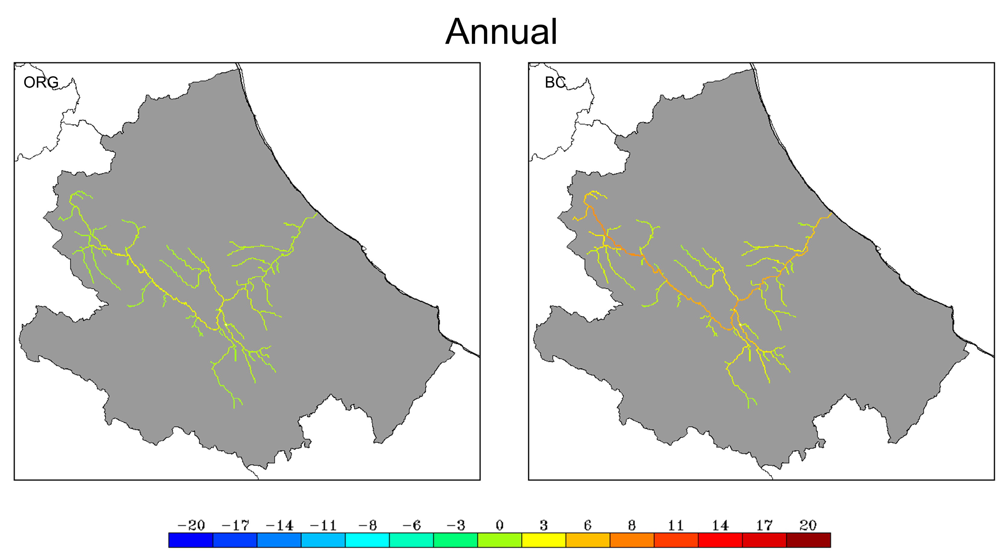
3.2.2. Hydrological Change Signal and Mean Discharge (MD-CS)

Pescara S. Teresa grid-node percentage Mean Discharge hydrological Change Signal (MD-CS) is shown in Figure 5c. The maximum discharge reduction is obtained in the summer where the future discharge flow is close to zero (Figure 5b). The ensemble mean changes for the RCP 8.5 (Figure 5, black tick lines) draw a characteristic annual pattern with a signal close to zero (However, with the opposite sign for January and February, +20% and −20%, respectively) during winter months and down to ~−40% in July. However, it is noteworthy that the large spread among the different CHyM runs, which characterizes the MD-CS except for the summer season (July and August) where all the hydrological simulations converge toward a large negative signal. A large spread characterizes the spring months, which ranges from ~−70% to ~+70% in May. In the same period, an alteration of the MD-CS produced by applying the bias correction can also be observed, which produces a reduction of the original negative MD-CS (from ~−40% to −20%). In this regard, it should be underlined that the impact of QM on the MD-CS is not directly connected to a QM impact on the precipitation CCS, which is mainly preserved, as shown in Figure 4a. At the same time, however, it can also be observed that the annual cycle of MD-CS is not altered by applying the QM on the driving climate simulations. Considering the MD-CS resulting from the RCP 4.5 (Figure 5c, left panel), slightly small changes in the monthly mean discharge can be observed. Two secondary dry peaks are found in the spring and the autumn, in addition to the primary one in the summer. For the RCP 4.5, the QM application, as we consider the ensemble average, does not impact the original MD-CS, except for the negative signal in June, which is dampened by the QM application.

In the following section, we present the spatial distribution of the MD-CS over the entire Pescara-Aterno basin.

In Figure 6 and Figure 7, the impact on the discharge variation in the Aterno-Pescara river network is shown in terms of percentage differences between a future 15-year period projection and a reference period of hydrological simulations. Warm colors in the maps represent increasing discharge from 2081 to 2095, while negative values drawn in blue-shades indicates a decrease. In the same figures, discharge changes obtained with original (ORG) and bias-adjusted (BC) climate simulations is reported considering the annual and seasonal basis for the RCP 8.5 and RCP 4.5 (Figure 6 and Figure 7, respectively).

According to the RCP 8.5 forcing (Figure 6), on an annual basis, a general discharge decrease is projected to range from ~−10% to ~−20%. Bias corrected climate simulation causes an overall smoothing of such variations, since the discharge decrease is lowered, especially in the small catchments placed in the north-western quarter of the Abruzzo region.

Deepening the analysis on a seasonal basis, discharge changes highlight a large variability among the different seasons. A general discharge increase is simulated in the winter, over the southern tributaries. However, a geographical pattern is emphasized, which results in increasing runoff rates over the Aterno sub-catchments and decreasing the contribution of the Pescara sub-catchment tributaries. This effect can be explained since the two sub-catchments’ characteristics are very different. The Aterno basin mainly lays over inter-mountain wide valleys and receives runoff contributions from the higher Apennines area. Therefore, a temperature increase causes an increment on the contribution of the snowmelt over this area, which results in a local discharge increase.

As underlined in the previous analysis, the summer season is the most affected by a consistent negative signal, down to −50% without highlighting spatial variability. Confirming point-scale results’ bias correction introduces a slightly wetter MD-CS. It means a reduction of the negative signal and an increase of the (rare) positive MD-CS. However, bias correction impacts differently over the different seasons and geographical portion of the basin. Considering the main river of the entire basin (Pescara river), a slight alteration of the original MD-CS is observed. However, in other seasons, the QM impact can be relevant.

In the winter season, especially in the north-western portion of the basin, a consistent increase of the original MD-CS, shifting from ~0 to ~+15–20% is found. In the summer season, the original MD-CS ~−40% is dampened to ~−30% while considering bias-corrected driven CHyM simulations. However, as observed in the point-scale analysis shown in Figure 5, the largest alteration of the original MD-CS is found in the spring season. Considering the original climate inputs, a significant discharge decrease is given over the whole drainage network, but this effect is heavily smoothed by the introduction of the bias-correction, where a change of the MD-CS sign (from negative to positive) in the north-western part of the basin occurred.

According to the RCP 4.5 (Figure 7), we observe a relevant dampening of the negative MD-CS in the spring and summer season observed in the RCP 8.5. Especially in the latter season, the negative signal ~−50% is halved in RCP 4.5 driven hydrological simulations. Additionally, in the RCP 4.5, QM produces a slightly wetter MD-CS. However, the alteration is lower than what resulted for the RCP 8.5, which is coherent with a lower MD-CS magnitude.

Lastly, the variability of the MD-CS produced by the individual hydrological run, corresponding to the individual driving RCM, has been investigated, as well as the related impact given by the application of the QM. In Figure 8, the annual MD-CS for the individual CHyM runs is reported, according to the original and bias corrected climate inputs (which consider RCP 8.5). QM produces wetter MD-CS in the individual CHyM run in all the ensemble members. However, the QM impact results in a different magnitude among the different CHyM runs. We can also observe how, in the small tributaries and river segments characterized by a torrential regime, MD-CS is the most impacted by the QM application. On the other hand, if we consider the longest river of the basin (Pescara), the impact of the QM is sensibly lower. These results highlight the importance of considering not only the ensemble mean MD-CS alteration, but also what QM produces on the individual ensemble member.

3.2.3. Hydrological Stress Change Signal (HS-CS)

In this section, the analysis on the expected Hydrologic Stress conditions Change Signal (HS-CS) is presented (Figure 9) for the RCP 8.5. Hydrological stress events are represented as the number of hours where the BDD index exceeds an empirically-derived threshold, as described in Section 2.3. The HS-CS is evaluated as the difference of the mean number of events characterizing the future period and the reference period.

Considering the CHyM runs’ ensemble mean, a slight HS-CS can be generally observed, which is different from the mean discharge that showed a larger change signal. A slight increase of the projected number of events can be observed (Figure 9) on an annual basis (~3) in the Aterno river, which results from the wetter signal observed for the mean discharge QM. Figure 9’s upper-right panel shows an increased HS-CS of approximately six events for the bias-corrected driven hydrological simulation in the future period over the two main rivers of the basin (Aterno river, in the western portion of the basin and Pescara river, which is perpendicular to the coast line). Similar to the mean discharge, the spring and autumn shows a large impact of the QM application on the original signal at a seasonal level. A similar HS-CS is obtained for RCP 4.5 (supplementary material Figure S3). However, the amplification of the HS-CS after QM application observed in the RCP 8.5 appears consistently smoothed in the RCP4.5. This different effect of the QM in the two different RCPs has been observed in the mean discharge change signal, mostly in the spring season.

In what follows, the HS-CS and related effects of the QM for each individual member of the hydrological simulations’ ensemble (Figure 10) are presented. This analysis is carried out in order to underline the inter-model variability of the hydrological stress signal, which provides a basic idea about the uncertainty related to the signal changes.

This aspect is particularly important, since HS-CS is mainly connected to severe-to-extreme precipitation. The ability to simulate severe-to-extreme precipitation is a function of the physical schemes and parameterization used by each driving climate simulation deeply affecting the representation of such events [76]. For the HS-CS, a consistent variability among the different driving RCMs is observed.

Considering original climate inputs, the inter-model HS-CS ranges from ~+15 events in the future period considering the CHyM CNRM-CM5-RCA4 driven, down to a negative HS-CS ~−10 of the CHyM MPI-ESM-LR-RCA4 driven. Considering the other driving RCMs, a slightly positive HS-CS in the Pescara river portion was obtained, considering the ICHEC-EC-EARTH_SMHI-RCA4 (~+6 events), as well as a low HS-CS (between 0 and +3 events) when considering the other two driving RCMs (IPSL-CM5A-MR-RCA4 and MOHC-HadGEM2-ES-RCA4).

Concerning CHyM simulations driven by the bias-corrected climate inputs, which is similar to the MD-CS, we obtained a slightly wetter ensemble mean signal (an increase of the positive signals) and a reduction of the negative signals, on an annual base. We can generally observe an increase of about three events in the HS-CS considering the bias-corrected RCM simulations.

However, focusing on the individual ensemble member, it is noteworthy that the strong amplification is obtained in the HS-CS of the CHyM MPI-ESM-LR-RCA4 driven in the Aterno river (north-western section of the Aterno-Pescra basin), where a HS-CS of ~+3 events is modified to ~+15 events when bias corrected climate input is considered.

4. Conclusions

In this study, we analyzed the response of the hydrology of a small catchment in Central Italy for the projected climate change at the end of the 21st century. Results from the original and statistically adjusted RCM simulations have been compared, according to a widely used bias correction technique (quantile mapping).

It follows a summary of the findings of the present study concerning both the climate and hydrological simulation results.

1- Original simulations largely overestimate wet-day frequency and underestimate 99th percentile precipitation (i.e., extreme precipitation) during the calibration period. The CCS, original simulations showed a negative signal for the wet-day frequency (down to –30% in the summer) and an increase of the 99th percentile precipitation (~15% on an annual base). Median precipitation CCS is generally small, in the range ± 5%. In this context, QM mainly preserved the original changes over the different statistics considered.

2- For the temperature, the original simulations showed an annual CCS from the median ~3.5–4 °C. During the summer season, CCS peaked up to 6 °C with a small inter-model spread. The temperature CCS is only slightly altered by QM with modifications generally in the range ± 0.5 °C considering the CCS of the median. A relevant exception is represented by the 5th percentile of the winter temperature (cold extremes), where a consistent reduction of the original CCS occurred (from 5.5 to 3.5, considering the median of the ensemble members distribution). Similarly, for the mountain sector of the study area, a considerable negative bias is found during the calibration period (up to –9 °C). These results have been obtained with regard to the RCP 8.5. According to the RCP 4.5, the CCS is generally halved due to the impact of the QM application.

Combining the resulting precipitation and temperature biases during the calibration period, particular care is suggested when original simulations are used for driving climate-impact modeling studies. In fact, climate simulation biases could implicitly (and not linearly) propagate into impact model results.

3- Regarding the hydrological simulations, the original climate input driven CHyM consistently overestimated (in the spring months) monthly mean discharge of the reference period, up to almost 100% considering the CHyM ensemble mean. However, very different results were obtained considering the different driving RCMs. As expected, QM, which consistently reduced these large biases during the spring months.

4- Original climate inputs driven by CHyM simulations produce a consistent drying of the mean discharge (down to −50% in the summer), according to the RCP 8.5. The winter season is the least affected season by drier conditions, which shows a positive MD-CS in the westernmost portion of the basin. Regarding what was observed for the temperature projected changes, the negative signal of the summer season is roughly halved when the RCP 4.5 is considered. On the other hand, events involving HS-CS indicated a very small change signal considering both the RCPs (+3 events in the future period on an annual basis, according to the RCP 8.5).

5- Concerning the impact of the climate inputs’ statistical adjustment, we obtained a slightly wetter signal (namely a decrease/increase of the negative/positive MD-CS) with bias-corrected climate inputs. This feature resulted in the MD-CS and HS-CS produced considering the ensemble mean and the individual CHyM runs. Spatially, the impact of the QM is found generally more remarkable in the western mountain portion of the domain, where rivers are characterized by a torrential regime than in the other areas. Concerning the spread among the individual CHyM runs, bias-corrected climate inputs do not increase, nor reduce, the variability of hydrological changes obtained with original climate inputs for both MD-CS and HS-CS.

Even if a hydrological change signal derived from bias-corrected climate inputs could be more trustworthy from an end-user’s perspective, many side considerations should be added to the provision of the climate/hydrological information. The variation generated on the original CCS and its propagation in the HCS should be carefully considered.

In this regard, in recent years, a considerable and sometimes controversial scientific debate has risen up over the plausibility of CCS alteration produced in the post-processing phase. Specifically, for the QM, the rationale behind modifying the original CCS relies on the assumption of climate model biases being time independent (time-stationary biases). Several authors have demonstrated that biases may be climate-state-dependent, which is different in a future climate [33,36,77]. In this context, QM impact is considered the result of mathematical artifacts and should be avoided. This occurs especially when QM is used for bias correcting and implicitly downscaling climate projections to finer-scale observations. In this regard, different studies used a QM configuration explicitly preserving original long-term trends of the climate variables [30,66,78]. However, in this latter case, an assumption is made and it regards the temporal non-stationary of the model biases, which can be physically questionable. Furthermore, to increase the complexity of the issue, raw model CCS can be, in turn, questionable when original simulations (as we observed in our study) are affected by large biases. In principle, they may originate implausible CCS (e.g., biases affecting the 5th percentile of the winter season temperature in our study case).

Concerning the discussed temporal stationarity of climate model biases, relatively temporal-stable biases have been found in several studies through pseudo-reality experiments [37,38,51,79]. Other studies, e.g., References [23,24,31], suggest that model biases are in good approximation when they are only dependent on the magnitude of simulated values, which indicates this feature as intensity-dependent biases. In this regard, References [31,34] provide an analytic description of how CCS modification produced by QM in the context of time-independent and intensity-dependent biases is a desirable effect of removing biases rather than consisting of mathematical artifacts.

Even if not addressed in this study, another important aspect to consider is the impact of QM on the original inter-dependencies between temperature and precipitation. There is a possibility for degradation of inter-variables’ physical relationships caused by a bias correction applied on an individual variable marginal distribution. Several studies address this issue by highlighting that traditional uni-variate QM does not degrade original simulated physical inter-variable dependencies [73,75,80]. However, a bi-variate QM configuration can positively affect hydrological simulations’ performance in complex-orography snow-dominated domains [81].

All these plausible arguments entrap bias correction into a dilemma. However, some general and useful considerations can be drawn regardless.

Original model simulations present substantial biases, which can non-linearly propagate into the impact model results. At least in the calibration period, bias-corrected simulations are physically much closer to the observed values, which allows a more representative simulation produced by the impact model (in our case, by the CHyM hydrological model). A heavily-biased climate simulation could potentially impact model results by generating a biased signal (both climate and hydrological). However, bias correction application is far from representing the solution for providing reliable information to end-users. The impact of QM must be carefully considered all over the methodological chain, from the calibration period to the modification produced in the impact model results going through the modification produced only on the signal of climate variables. Furthermore, where the size of the observed products is sufficient, a cross-validation should be performed to test the capability of the QM of improving climate and impact model simulations over an independent time segment (i.e., not used for the calibration of the QM correction functions). However, in this regard, serious concern about the plausibility and suitability of the current procedures used for evaluating the added value of bias correction techniques have been recently raised [82]. In any context, statistical bias correction approaches rely on the quality of the original RCM simulations which, in turn, represent a dynamic downscaling of GCM, dependent on the quality of the large-scale forcing of the GCM [83]. Hence, for a reliable climate input in impact studies, it is essential that the RCMs correctly captures a regional-scale response to the driving large-scale processes and realistically represents the relative long-term changes.

Climate science has the ethical task of providing information to which real actions undertaken in the different fields impacted by climate change will correspond. Given that, climate scenarios’ communication should rely on the availability of both original and statistically adjusted climate projections and related impacts joined with a clear description of concerns, strengths, and weakness regarding both the products.

References

1. Seneviratne, S.I.; Corti, T.; Davin, E.L.; Hirschi, M.; Jaeger, E.B.; Lehner, I.; Orlowsky, B.; Teuling, A.J. Investigating soil moisture-climate interactions in a changing climate: A review. Earth Sci. Rev. 2010, 99, 125–161. [Google Scholar] [CrossRef]
2. Drobinski, P.; Da Silva, N.; Panthou, G.; Bastin, S.; Muller, C.; Ahrens, B.; Borga, M.; Conte, D.; Fosser, G.; Giorgi, F.; et al. Scaling precipitation extremes with temperature in the Mediterranean: Past climate assessment and projection in anthropogenic scenarios. Clim. Dyn. 2016. [Google Scholar] [CrossRef] [Green Version]
3. Trenberth, K.E. Conceptual framework for changes of extreme of the hydrological cycle with climate change. Clim. Chang. 1999, 42, 327–339. [Google Scholar] [CrossRef]
4. Lionello, P.; Dalan, F.; Elvini, E. Cyclones in the Mediterranean region: The present and the doubled CO2 climate scenarios. Clim. Res. 2002, 22, 147–159. [Google Scholar] [CrossRef]
5. Mariotti, A.; Zeng, N.; Lau, K.M. Euro-Mediterranean rainfall and ENSO-A seasonally varying relationship. Geophys. Res. Lett. 2002, 29, 2–5. [Google Scholar] [CrossRef] [Green Version]
6. Lorenz, D.J.; DeWeaver, E.T. The response of the extratropical hydrological cycle to global warming. J. Clim. 2007, 20, 3470–3484. [Google Scholar] [CrossRef]
7. Liu, S.C.; Fu, C.; Shiu, C.-J.; Chen, J.-P.; Wu, F. Temperature dependence of global precipitation extremes. Geophys. Res. Lett. 2009, 36, 1–4. [Google Scholar] [CrossRef] [Green Version]
8. Giorgi, F.; Im, E.-S.; Coppola, E.; Diffenbaugh, N.S.; Gao, X.J.; Mariotti, L.; Shi, Y. Higher Hydroclimatic Intensity with Global Warming. J. Clim. 2011, 24, 5309–5324. [Google Scholar] [CrossRef]
9. Scoccimarro, E.; Gualdi, S.; Navarra, A. Heavy precipitation events over the Euro-Mediterranean region in a warmer climate: Results from CMIP5 models. Reg. Environ. Chang. 2016, 595–602. [Google Scholar] [CrossRef]
10. Gao, X.; Giorgi, F. Increased aridity in the Mediterranean region under greenhouse gas forcing estimated from high resolution simulations with a regional climate model. Glob. Planet. Chang. 2008, 62, 195–209. [Google Scholar] [CrossRef]
11. Giorgi, F.; Lionello, P. Climate change projections for the Mediterranean region. Glob. Planet. Chang. 2008, 63, 90–104. [Google Scholar] [CrossRef]
12. Giorgi, F. Climate change hot-spots. Geophys. Res. Lett. 2006, 33, 1–4. [Google Scholar] [CrossRef]
13. Hagemann, S.; Chen, C.; Haerter, J.O.; Heinke, J.; Gerten, D.; Piani, C. Impact of a Statistical Bias Correction on the Projected Hydrological Changes Obtained from Three GCMs and Two Hydrology Models. J. Hydrometeorol. 2011, 12, 556–578. [Google Scholar] [CrossRef]
14. Mbaye, M.L.; Haensler, A.; Hagemann, S.; Gaye, A.T.; Moseley, C.; Afouda, A. Impact of statistical bias correction on the projected climate change signals of the regional climate model REMO over the Senegal River Basin. Int. J. Climatol. 2016, 36, 2035–2049. [Google Scholar] [CrossRef] [Green Version]
15. Lenderink, G.; Buishand, A.; van Deursen, W. Estimates of future discharges of the river Rhine using two scenario methodologies: Direct versus delta approach. Hydrol. Earth Syst. Sci. 2007, 11, 1145–1159. [Google Scholar] [CrossRef]
16. Coppola, E.; Verdecchia, M.; Giorgi, F.; Colaiuda, V.; Tomassetti, B.; Lombardi, A. Changing hydrological conditions in the Po basin under global warming. Sci. Total Environ. 2014, 493, 1183–1196. [Google Scholar] [CrossRef]
17. Chiew, F.H.S.; Kirono, D.G.C.; Kent, D.M.; Frost, A.J.; Charles, S.P.; Timbal, B.; Nguyen, K.C.; Fu, G. Comparison of runoff modelled using rainfall from different downscaling methods for historical and future climates. J. Hydrol. 2010, 387, 10–23. [Google Scholar] [CrossRef]
18. Ravazzani, G.; Barbero, S.; Salandin, A.; Senatore, A.; Mancini, M. An integrated Hydrological Model for Assessing Climate Change Impacts on Water Resources of the Upper Po River Basin. Water Resour. Manag. 2014, 29, 1193–1215. [Google Scholar] [CrossRef]
19. Vezzoli, R.; Mercogliano, P.; Pecora, S.; Zollo, A.L.; Cacciamani, C. Hydrological simulation of po river (North Italy) discharge under climate change scenarios using the RCM COSMO-CLM. Sci. Total Environ. 2015, 521–522, 346–358. [Google Scholar] [CrossRef]
20. Giorgi, F. Simulation of regional climate using a limited area model nested in a general circulation model. J. Clim. 1990, 3, 941–963. [Google Scholar] [CrossRef] [Green Version]
21. Giorgi, F.; Mearns, L.O. Introduction to special section: Regional Climate Modeling Revisited. J. Geophys. Res. 1999, 104, 6335. [Google Scholar] [CrossRef]
22. Grassi, B.; Redaelli, G.; Visconti, G. Arctic sea ice reduction and extreme climate events over the mediterranean region. J. Clim. 2013, 26, 10101–10110. [Google Scholar] [CrossRef]
23. Boberg, F.; Christensen, J.H. Overestimation of Mediterranean summer temperature projections due to model deficiencies. Nat. Clim. Chang. 2012, 2, 433–436. [Google Scholar] [CrossRef]
24. Christensen, J.H.; Boberg, F.; Christensen, O.B.; Lucas-Picher, P. On the need for bias correction of regional climate change projections of temperature and precipitation. Geophys. Res. Lett. 2008, 35, L20709. [Google Scholar] [CrossRef]
25. Bellprat, O.; Kotlarski, S.; Lüthi, D.; Schär, C. Physical constraints for temperature biases in climate models. Geophys. Res. Lett. 2013, 40, 4042–4047. [Google Scholar] [CrossRef]
26. Casati, B.; Yagouti, A.; Chaumont, D. Regional climate projections of extreme heat events in nine pilot Canadian communities for public health planning. J. Appl. Meteorol. Climatol. 2013, 52, 2669–2698. [Google Scholar] [CrossRef]
27. Themeßl, M.J.; Gobiet, A.; Heinrich, G. Empirical-statistical downscaling and error correction of regional climate models and its impact on the climate change signal. Clim. Chang. 2011, 112, 449–468. [Google Scholar] [CrossRef]
28. Dosio, A.; Paruolo, P.; Rojas, R. Bias correction of the ENSEMBLES high resolution climate change projections for use by impact models: Analysis of the climate change signal. J. Geophys. Res. Atmos. 2012, 117, 1–24. [Google Scholar] [CrossRef] [Green Version]
29. Maurer, E.P.; Pierce, D.W. Bias correction can modify climate model simulated precipitation changes without adverse effect on the ensemble mean. Hydrol. Earth Syst. Sci. 2014, 18, 915–925. [Google Scholar] [CrossRef] [Green Version]
30. Cannon, A.J.; Sobie, S.R.; Murdock, T.Q. Bias correction of GCM precipitation by quantile mapping: How well do methods preserve changes in quantiles and extremes? J. Clim. 2015, 28, 6938–6959. [Google Scholar] [CrossRef]
31. Gobiet, A.; Suklitsch, M.; Heinrich, G. The effect of empirical-statistical correction of Intensity-Dependent model errors on the climate change signal. Hydrol. Earth Syst. Sci. Discuss. 2015, 12, 5671–5701. [Google Scholar] [CrossRef]
32. Pierce, D.W.; Cayan, D.R.; Maurer, E.P.; Abatzoglou, J.T.; Hegewisch, K.C. Improved bias correction techniques for hydrological simulations of climate change. J. Hydrometeorol. 2015, 150915153707007. [Google Scholar] [CrossRef]
33. Maraun, D. Bias Correcting Climate Change Simulations - A Critical Review. Curr. Clim. Chang. Rep. 2016, 1–10. [Google Scholar] [CrossRef] [Green Version]
34. Ivanov, M.A.; Luterbacher, J.; Kotlarski, S.; Ivanov, M.A.; Luterbacher, J.; Kotlarski, S. Climate Model Biases and Modification of the Climate Change Signal by Intensity-Dependent Bias Correction. J. Clim. 2018, 6591–6610. [Google Scholar] [CrossRef]
35. Sangelantoni, L.; Russo, A.; Gennaretti, F. Impact of bias correction and downscaling through quantile mapping on simulated climate change signal: A case study over Central Italy. Theor. Appl. Climatol. 2019, 135, 725–740. [Google Scholar] [CrossRef]
36. Switanek, M.B.; Troch, P.A.; Castro, C.L.; Leuprecht, A.; Chang, H. Scaled distribution mapping: A bias correction method that preserves raw climate model projected changes. Hydrol. Earth Syst. Sci. 2017, 21, 2649–2666. [Google Scholar] [CrossRef] [Green Version]
37. Maraun, D. Nonstationarities of regional climate model biases in European seasonal mean temperature and precipitation sums. Geophys. Res. Lett. 2012, 39, 1–5. [Google Scholar] [CrossRef] [Green Version]
38. Teutschbein, C.; Seibert, J. Is bias correction of regional climate model (RCM) simulations possible for non-stationary conditions. Hydrol. Earth Syst. Sci. 2013, 17, 5061–5077. [Google Scholar] [CrossRef] [Green Version]
39. Maraun, D.; Shepherd, T.G.; Widmann, M.; Zappa, G.; Walton, D.; Gutiérrez, J.M.; Hagemann, S.; Richter, I.; Soares, P.M.M.; Hall, A.; et al. Towards process-informed bias correction of climate change simulations. Nat. Clim. Chang. 2017, 7, 764–773. [Google Scholar] [CrossRef] [Green Version]
40. Grenier, P. Two types of physical inconsistency to avoid with univariate quantile mapping: A case study over North America concerning relative humidity and its parent variables. J. Appl. Meteorol. Climatol. 2018, 57, 347–364. [Google Scholar] [CrossRef]
41. Moss, R.H.; Edmonds, J.A.; Hibbard, K.A.; Manning, M.R.; Rose, S.K.; van Vuuren, D.P.; Carter, T.R.; Emori, S.; Kainuma, M.; Kram, T.; et al. The next generation of scenarios for climate change research and assessment. Nature 2010, 463, 747–756. [Google Scholar] [CrossRef] [PubMed]
42. Thomson, A.M.; Calvin, K.V.; Smith, S.J.; Kyle, G.P.; Volke, A.; Patel, P.; Delgado-Arias, S.; Bond-Lamberty, B.; Wise, M.A.; Clarke, L.E.; et al. RCP4.5: A pathway for stabilization of radiative forcing by 2100. Clim. Chang. 2011, 109, 77–94. [Google Scholar] [CrossRef] [Green Version]
43. Meinshausen, M.; Smith, S.J.; Calvin, K.; Daniel, J.S.; Kainuma, M.L.T.; Lamarque, J.-F.; Matsumoto, K.; Montzka, S.A.; Raper, S.C.B.; Riahi, K.; et al. The RCP greenhouse gas concentrations and their extensions from 1765 to 2300. Clim. Chang. 2011, 109, 213–241. [Google Scholar] [CrossRef] [Green Version]
44. Dankers, R.; Feyen, L. Flood hazard in Europe in an ensemble of regional climate scenarios. J. Geophys. Res. Atmos. 2009, 114, 1–16. [Google Scholar] [CrossRef]
45. Dobler, C.; Bürger, G.; Stötter, J. Assessment of climate change impacts on flood hazard potential in the Alpine Lech watershed. J. Hydrol. 2012, 460–461, 29–39. [Google Scholar] [CrossRef]
46. Feyen, L.; Dankers, R.; Bodis, K.; Salamon, P.; Barredo, J. Flood hazard in Europe in an ensemble of regional climate scenarios. Clim. Chang. 2012, 112, 47–62. [Google Scholar] [CrossRef]
47. Blöschl, G.; Hall, J.; Viglione, A.; Perdigão, R.A.P.; Parajka, J.; Merz, B.; Lun, D.; Arheimer, B.; Aronica, G.T.; Bilibashi, A.; et al. Changing climate both increases and decreases European river floods. Nature 2019, 573, 108–111. [Google Scholar] [CrossRef]
48. Alfieri, L.; Burek, P.; Feyen, L.; Forzieri, G. Global warming increases the frequency of river floods in Europe. Hydrol. Earth Syst. Sci. 2015, 19, 2247–2260. [Google Scholar] [CrossRef] [Green Version]
49. Themeßl, M.J.; Gobiet, A.; Leuprecht, A. Empirical-statistical downscaling and error correction of daily precipitation from regional climate models. Int. J. Climatol. 2011, 1544, 1530–1544. [Google Scholar] [CrossRef]
50. Rajczak, J.; Kotlarski, S.; Salzmann, N.; Schär, C. Robust climate scenarios for sites with sparse observations: A two-step bias correction approach. Int. J. Climatol. 2015, 36, 1226–1243. [Google Scholar] [CrossRef] [Green Version]
51. Ivanov, M.A.; Kotlarski, S. Assessing distribution-based climate model bias correction methods over an alpine domain: Added value and limitations. Int. J. Climatol. 2017, 37, 2633–2653. [Google Scholar] [CrossRef]
52. Jacob, D.; Petersen, J.; Eggert, B.; Alias, A.; Christensen, O.B.; Bouwer, L.M.; Braun, A.; Colette, A.; Déqué, M.; Georgievski, G.; et al. Euro-CORDEX: New high-resolution climate change projections for European impact research. Reg. Environ. Chang. 2014, 14, 563–578. [Google Scholar] [CrossRef]
53. Haylock, M.R.; Hofstra, N.; Klein Tank, A.M.G.; Klok, E.J.; Jones, P.D.; New, M. A European daily high-resolution gridded data set of surface temperature and precipitation for 1950-2006. J. Geophys. Res. Atmos. 2008, 113. [Google Scholar] [CrossRef] [Green Version]
54. Hofstra, N.; Haylock, M.; New, M.; Jones, P.D. Testing E-OBS European high-resolution gridded data set of daily precipitation and surface temperature. J. Geophys. Res. Atmos. 2009, 114. [Google Scholar] [CrossRef]
55. Cornes, R.C.; van der Schrier, G.; van den Besselaar, E.J.M.; Jones, P.D. An Ensemble Version of the E-OBS Temperature and Precipitation Data Sets. J. Geophys. Res. Atmos. 2018, 123, 9391–9409. [Google Scholar] [CrossRef] [Green Version]
56. Li, J.; Johnson, F.; Evans, J.; Sharma, A. A comparison of methods to estimate future sub-daily design rainfall. Adv. Water Resour. 2017, 110, 215–227. [Google Scholar] [CrossRef]
57. Tomassetti, B.; Coppola, E.; Verdecchia, M.; Visconti, G. Coupling a distributed grid based hydrological model and MM5 meteorological model for flooding alert mapping. Adv. Geosci. 2005, 2, 59–63. [Google Scholar] [CrossRef] [Green Version]
58. Verdecchia, M.; Coppola, E.; Faccani, C.; Ferretti, R.; Memmo, A.; Montopoli, M.; Rivolta, G.; Paolucci, T.; Picciotti, E.; Santacasa, A.; et al. Flood forecast in complex orography coupling distributed hydro-meteorological models and in-situ and remote sensing data. Meteorol. Atmos. Phys. 2008, 101, 267–285. [Google Scholar] [CrossRef]
59. Verdecchia, M.; Coppola, E.; Tomassetti, B.; Visconti, G. Cetemps Hydrological Model (CHyM), a Distributed Grid-Based Model Assimilating Different Rainfall Data Sources. In Hydrological Modelling and the Water Cycle; Sorooshian, S., Hsu, K.L., Coppola, E., Tomassetti, B., Verdecchia, M., Visconti, G., Eds.; Springer: Berlin/Heidelberg, Germany, 2009; Volume 63, pp. 165–201. [Google Scholar]
60. Thornthwaite, C.W.; Mather, J.R. Instructions and Tables for Computing Potential Evapotranspiration and the Water Balance; Publications in Climatology: Centerton, NJ, USA, 1957; Volume 10. [Google Scholar]
61. Wolfram, S. Statistical mechanics of cellular automata. Rev. Mod. Phys. 1983, 55, 601–644. [Google Scholar] [CrossRef]
62. Coppola, E.; Tomassetti, B.; Mariotti, L.; Verdecchia, M.; Visconti, G. Cellular automata algorithms for drainage network extraction and rainfall data assimilation. Hydrol. Sci. J. 2007, 52, 579–592. [Google Scholar] [CrossRef] [Green Version]
63. Di Baldassarre, G.; Montanari, A. Uncertainty in river discharge observations: A quantitative analysis. Hydrol. Earth Syst. Sci. 2009, 13, 913–921. [Google Scholar] [CrossRef] [Green Version]
64. Alfieri, L.; Pappenberger, F.; Wetterhall, F. The extreme runoff index for flood early warning in Europe. Nat. Hazards Earth Syst. Sci. 2014, 14, 1505–1515. [Google Scholar] [CrossRef] [Green Version]
65. Alfieri, L.; Thielen, J. A European precipitation index for extreme rain-storm and flash flood early warning. Meteorol. Appl. 2015, 22, 3–13. [Google Scholar] [CrossRef] [Green Version]
66. Ravazzani, G.; Bocchiola, D.; Groppelli, B.; Soncini, A.; Rulli, M.C.; Colombo, F.; Mancini, M.; Rosso, R. Simulation continue de l’écoulement fluvial pour l’estimation de l’indice de crue dans un bassin alpin du Nord de l’Italie. Hydrol. Sci. J. 2015, 60, 1013–1025. [Google Scholar] [CrossRef] [Green Version]
67. Ferretti, R.; Lombardi, A.; Tomassetti, B.; Sangelantoni, L.; Colaiuda, V.; Mazzarella, V.; Maiello, I.; Verdecchia, M.; Redaelli, G. Regional ensemble forecast for early warning system over small Apennine catchments on Central Italy. Hydrol. Earth Syst. Sci. Discuss. 2019, 1–25. [Google Scholar] [CrossRef] [Green Version]
68. Taraglio, S.; Chiesa, S.; La Porta, L.; Pollino, M.; Verdecchia, M.; Tomassetti, B.; Colaiuda, V.; Lombardi, A. Decision Support System for smart urban management: Resilience against natural phenomena and aerial environmental assessment. Int. J. Sustain. Energy Plan. Manag. 2019, 24, 135–146. [Google Scholar]
69. Singh, V.P.; Frevert, D.K. Mathematical Models of Small Watershed Hydrology and Application; Singh, V.P., Frevert, D.K., Eds.; Water Resources Publications: Highlands Ranch, CO, USA, 2002. [Google Scholar]
70. Thielen, J.; Bartholmes, J.; Ramos, M.H.; de Roo, A. The European Flood Alert System—Part 1: Concept and development. Hydrol. Earth Syst. Sci 2009, 13, 125–140. [Google Scholar] [CrossRef] [Green Version]
71. Boé, J.; Terray, L.; Habets, F.; Martin, E. Statistical and dynamical downscaling of the Seine basin climate for hydro-meteorological studies. Int. J. Climatol. 2007, 1655, 1643–1655. [Google Scholar] [CrossRef]
72. Déqué, M. Frequency of precipitation and temperature extremes over France in an anthropogenic scenario: Model results and statistical correction according to observed values. Glob. Planet. Chang. 2007, 57, 16–26. [Google Scholar] [CrossRef]
73. Gennaretti, F.; Sangelantoni, L.; Grenier, P. Toward daily climate scenarios for Canadian Arctic coastal zones with more realistic temperature-precipitation interdependence. J. Geophys. Res. Atmos. 2015, 120, 11–862. [Google Scholar] [CrossRef]
74. Teutschbein, C.; Seibert, J. Bias correction of regional climate model simulations for hydrological climate-change impact studies: Review and evaluation of different methods. J. Hydrol. 2012, 456–457, 12–29. [Google Scholar] [CrossRef]
75. Wilcke, R.A.I.; Mendlik, T.; Gobiet, A. Multi-variable error correction of regional climate models. Clim. Chang. 2013, 120, 871–887. [Google Scholar] [CrossRef] [Green Version]
76. Sillmann, J.; Kharin, V.V.; Zhang, X.; Zwiers, F.W.; Bronaugh, D. Climate extremes indices in the CMIP5 multimodel ensemble: Part 1. Model evaluation in the present climate. J. Geophys. Res. Atmos. 2013, 118, 1716–1733. [Google Scholar] [CrossRef]
77. Maraun, D. Bias Correction, Quantile Mapping, and Downscaling: Revisiting the Inflation Issue. J. Clim. 2013, 26, 2137–2143. [Google Scholar] [CrossRef] [Green Version]
78. Hempel, S.; Frieler, K.; Warszawski, L.; Schewe, J.; Piontek, F. A trend-preserving bias correction—The ISI-MIP approach. Earth Syst. Dyn. 2013, 4, 219–236. [Google Scholar] [CrossRef] [Green Version]
79. Räty, O.; Räisänen, J.; Ylhäisi, J.S. Evaluation of delta change and bias correction methods for future daily precipitation: Intermodel cross-validation using ENSEMBLES simulations. Clim. Dyn. 2014, 2287–2303. [Google Scholar] [CrossRef]
80. Räty, O.; Räisänen, J.; Bosshard, T.; Donnelly, C. Intercomparison of Univariate and Joint Bias Correction Methods in Changing Climate from a Hydrological Perspective. Climate 2018, 6, 33. [Google Scholar] [CrossRef] [Green Version]
81. Meyer, J.; Kohn, I.; Stahl, K.; Hakala, K.; Seibert, J.; Cannon, A.J. Effects of univariate and multivariate bias correction on hydrological impact projections in alpine catchments. Hydrol. Earth Syst. Sci. Discuss. 2018, 1–22. [Google Scholar] [CrossRef] [Green Version]
82. Maraun, D.; Widmann, M. Statistical Downscaling and Bias Correction for Climate Research; Cambridge University Press: Cambridge, UK, 2018; ISBN 9781107588783. [Google Scholar]
83. Sangelantoni, L.; Ferretti, R.; Redaelli, G. Toward a Regional-Scale Seasonal Climate Prediction System over Central Italy based on Dynamical Downscaling. Climate 2019, 7, 120. [Google Scholar] [CrossRef] [Green Version]
Figure 1. Aterno-Pescara river basin with the Abruzzo region boarders (Central Italy).
Atmosphere 10 00799 g001
Figure 2. Location of the Abruzzo region observational sites and a representative RCM grid. Magenta circles indicate sites providing observed time series of both temperature and precipitation.
Atmosphere 10 00799 g002
Figure 3. Original (a,c) and bias corrected (b,d) annual precipitation (a,b) and temperature (c,d) statistical distributions (PDFs) over the 17 reference sites for the calibration (or reference) period 2002-2016. On the tables at the right of the figures, we report biases over three statistics: wet-day frequency (WDF), median (ρ50), and the 99th percentile (ρ99) for precipitation and 5th, 50th, and 95th percentiles for the temperature. Simulations shown belong to a representative RCM (CNRM-CM5-RCA4).
Atmosphere 10 00799 g003aAtmosphere 10 00799 g003b
Figure 4. Original (ORG, blue box plots) and bias corrected (BC, red box plots) climate change signals (CCSs) for precipitation (a) and temperature (b). CCSs are reported on an annual (upper panels), winter season (central panels), and summer season (bottom panels). For each variable, CCS is defined over three statistics. For the precipitation, wet-day frequency (WDF), 50th and 99th percentiles. For the temperature, over 5th, 50th, and 95th percentiles. Box plots represent the statistical distribution built on the CCSs produced by the five RCMs over the 17 reference sites (5 RCMs * 17 reference sites = 85 values). On each box, quartiles (central mark and box edges), values within the 1.5 interquartile range from the box edges (whiskers), and outliers (plus signs) are shown. Results are shown for the RCP 8.5.
Atmosphere 10 00799 g004aAtmosphere 10 00799 g004b
Figure 5. Monthly mean discharge for the reference period (a) and future period (b) and the percentage difference between the two periods (c). In the left column hydrological simulations consider RCP 4.5 and in the right column RCP 8.5. In all the panels, dashed (solid) lines indicate CHyM simulations forced by original (bias-corrected) climate simulations. Black thick lines represent the CHyM simulation ensembles. In the upper panels, a red tick line represents the CHyM simulation driven by the reference period observed for the precipitation and temperature. Hydrological simulations have been extracted at the nearest grid node to the station of S. Teresa located in correspondence of the Pescara river mouth.
Atmosphere 10 00799 g005
Figure 6. Spatial distribution of mean discharge flow percentage changes on an annual and a seasonal basis, according to the RCP 8.5 emission scenario. Original (ORG) and bias corrected (BC) climate inputs are considered.
Atmosphere 10 00799 g006
Figure 7. Same as in Figure 6, but according to the RCP 4.5.
Atmosphere 10 00799 g007
Figure 8. Percentage annual MD-CS for the individual CHyM runs according to the RCP 8.5. Original climate inputs and bias-corrected climate inputs are reported in the upper and bottom panels, respectively.
Atmosphere 10 00799 g008
Figure 9. Spatial distribution of the BDD index changes, on an annual and seasonal basis, defined as the difference between the number of events characterizing the future period and the reference period. Results considering the RCP 8.5 are shown. Original (ORG) and bias corrected (BC) climate inputs are considered.
Atmosphere 10 00799 g009aAtmosphere 10 00799 g009b
Figure 10. Similar to Figure 8 but for the BDD index representing the HS-CS.
Atmosphere 10 00799 g010