Chemical Composition of Aerosol over the Arctic Ocean from Summer ARctic EXpedition (AREX) 2011–2012 Cruises: Ions, Amines, Elemental Carbon, Organic Matter, Polycyclic Aromatic Hydrocarbons, n-Alkanes, Metals, and Rare Earth Elements

 , ,
, ,
Abstract
:1. Introduction
2. Experiments
2.1. Sampling Campaigns
2.2. Sample Extraction and Analysis
2.2.1. PAHs and n-Alkanes
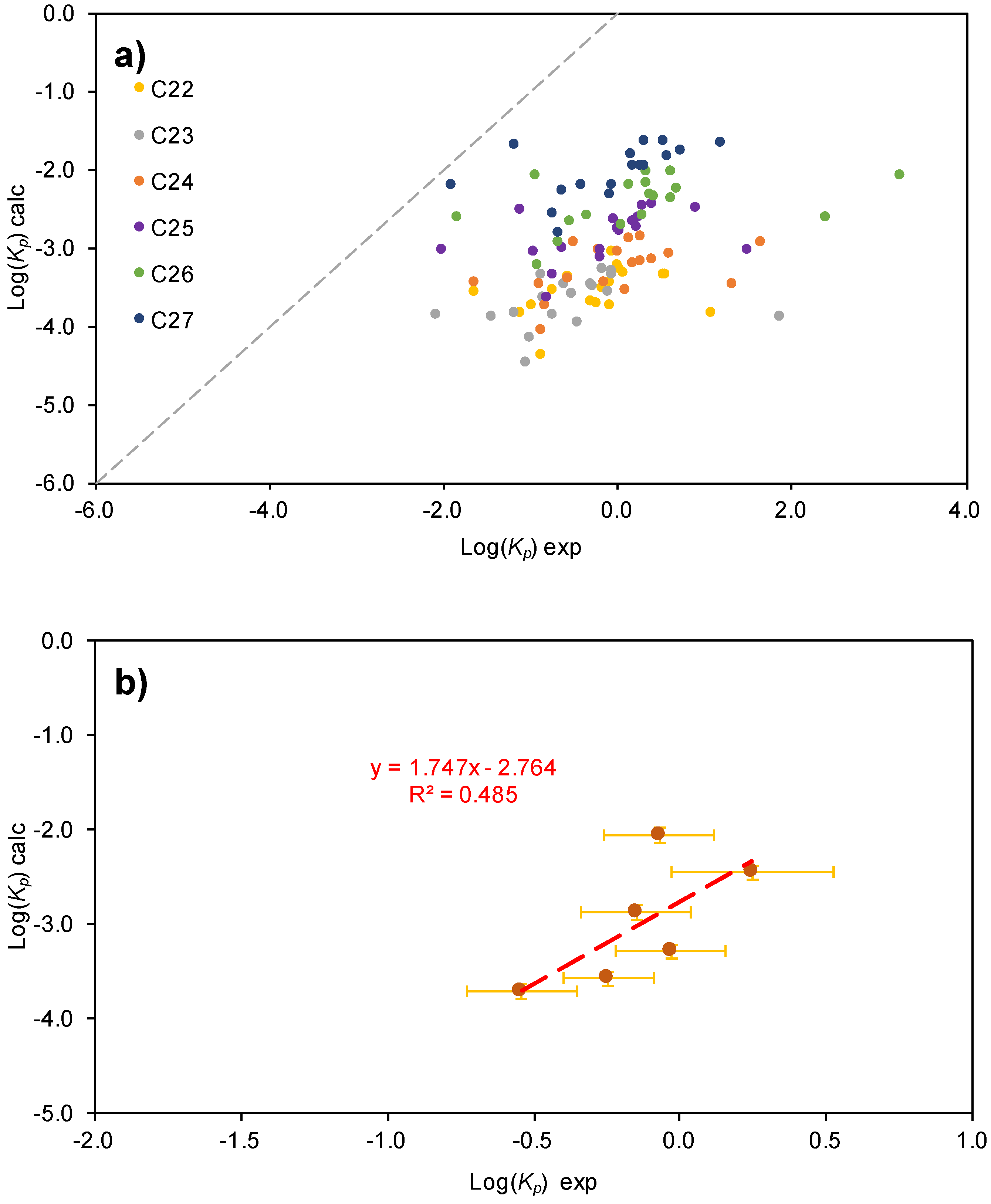
2.2.2. PAHs Gas/Particle Partitioning
2.2.3. Water-Soluble Compounds
2.2.4. OC, EC, and Metals
2.3. Back Trajectories and Copernicus Atmosphere Monitoring Service Data
3. Results
3.1. Water-Soluble Species
3.1.1. Water-Soluble Inorganic Ions
3.1.2. Water-Soluble Organic Ions
3.2. Carbonaceous Material And Full Chemical Composition
3.3. PAHs and n-Alkanes
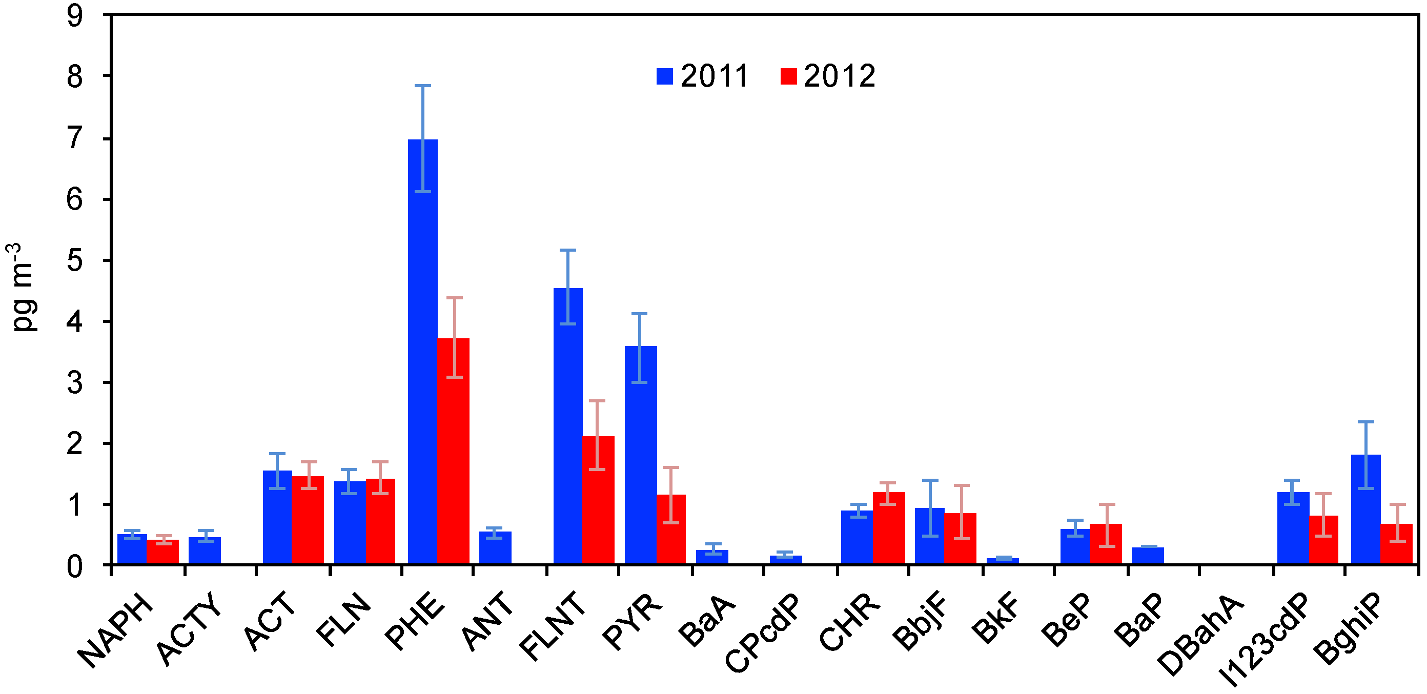
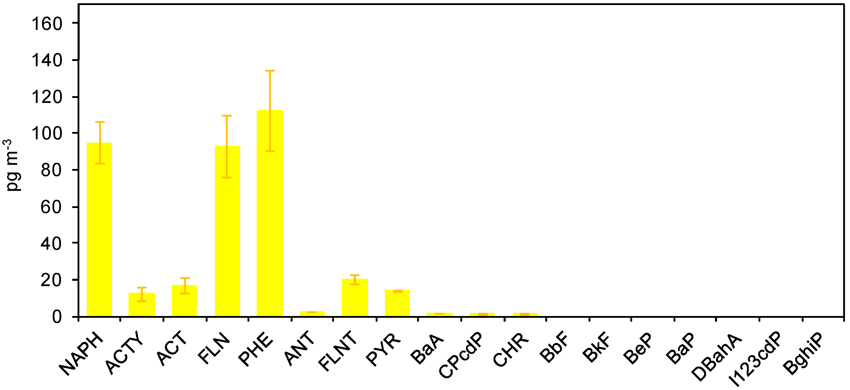
3.3.1. PAHs
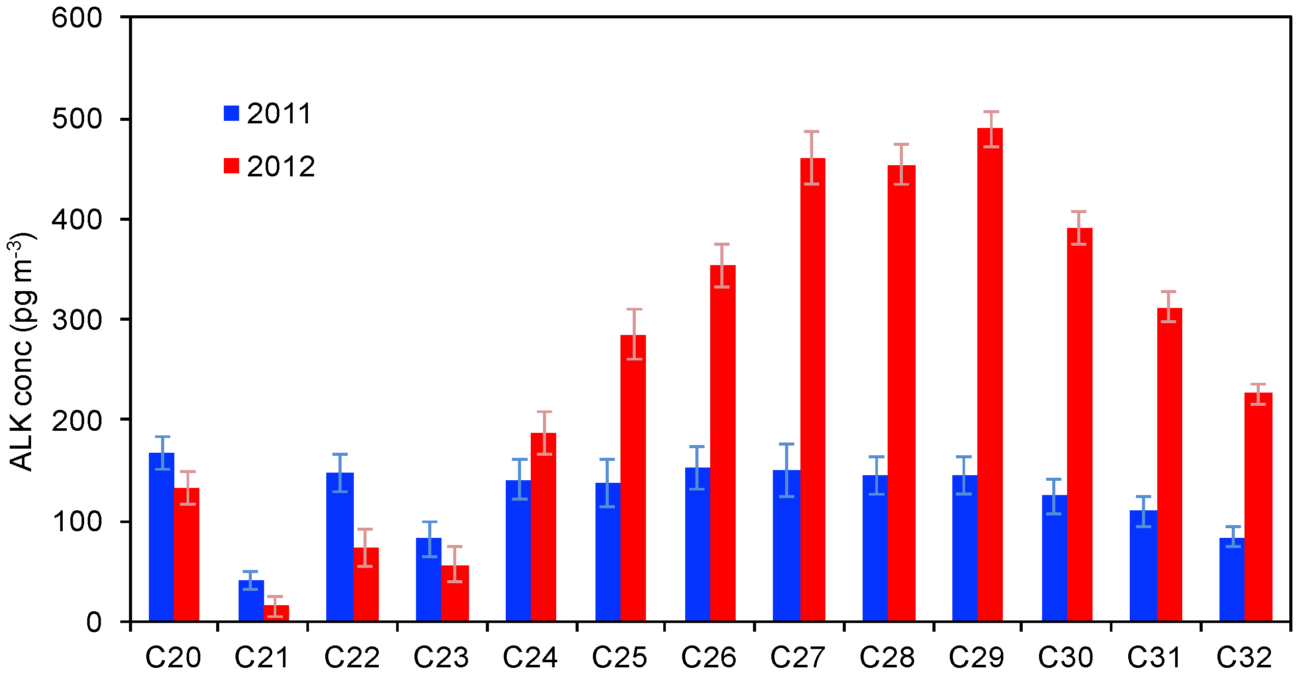
3.3.2. Alkanes
3.4. Element Concentrations
4. Conclusions
Supplementary Materials
Author Contributions
Funding
Acknowledgments
Conflicts of Interest
References
- IPCC. Climate Change 2013: The Physical Science Basis; Cambridge University Press: Cambridge, UK; New York, NY, USA, 2013. [Google Scholar]
- Serreze, M.C.; Barrett, A.P.; Stroeve, J.C.; Kindig, D.N.; Holland, M.M. The emergence of surface-based Arctic amplification. Cryosphere 2009, 3, 11–19. [Google Scholar] [CrossRef] [Green Version]
- Shindell, D.; Faluvegi, G. Climate response to regional radiative forcing during the twentieth century. Nat. Geosci. 2009, 2, 294–300. [Google Scholar] [CrossRef]
- Bond, T.C.; Doherty, S.J.; Fahey, D.W.; Forster, P.M.; Berntsen, T.; Deangelo, B.J.; Flanner, M.G.; Ghan, S.; Kärcher, B.; Koch, D.; et al. Bounding the role of black carbon in the climate system: A scientific assessment. J. Geophys. Res. 2013, 118, 1–173. [Google Scholar] [CrossRef]
- Ramanathan, V.; Feng, Y. Air pollution, greenhouse gases and climate change: Global and regional perspectives. Atmos. Environ. 2009, 43, 37–50. [Google Scholar] [CrossRef]
- Koren, I.; Kaufman, Y.J.; Remer, L.A.; Martins, J.V. Measurements of the effect of amazon smoke on inhibition of cloud formation. Science 2004, 303, 1342–1345. [Google Scholar] [CrossRef] [PubMed]
- Koren, I.; Martins, J.V.; Remer, L.A.; Afargan, H. Smoke invigoration versus inhibition of clouds over the amazon. Science 2008, 321, 946–949. [Google Scholar] [CrossRef] [PubMed]
- Kaufman, Y.J.; Tanré, D.; Boucher, O. A satellite view of aerosols in the climate system. Nature 2002, 419, 215–223. [Google Scholar] [CrossRef] [PubMed]
- Navarro, J.C.A.; Varma, V.; Riipinen, I.; Seland, Ø.; Kirkevag, A.; Struthers, H.; Iversen, T.; Hansson, H.-C.; Ekman, A.M.L. Amplification of Arctic warming by past air pollution reductions in Europe. Nat. Geosci. 2016. [Google Scholar] [CrossRef]
- Maturilli, M.; Herber, H.; Konig-Langlo, G. Surface radiation climatology for Ny-Ålesund, Svalbard (78.9° N), basic observations for trend detection. Theor. Appl. Climatol. 2015, 120, 331–339. [Google Scholar] [CrossRef]
- Isaksen, K.; Nordli, Ø.; FØrland, E.J.; Lupikasza, E.; Eastwood, S.; Niedzwiedz, T. Recent warming on Spitzbergen—Influence of atmospheric circulation and sea ice cover. J. Geophys. Res. Atmos. 2016. [Google Scholar] [CrossRef]
- Ødemark, K.; Dalsøren, S.B.; Samset, B.H.; Berntsen, T.K.; Fuglestvedt, J.S.; Myhre, G. Short-lived climate forcers from current shipping and petroleum activities in the Arctic. Atmos. Chem. Phys. 2012, 12, 1979–1993. [Google Scholar] [CrossRef] [Green Version]
- Shindell, D.; Kuylenstierna, J.C.I.; Vignati, E.; Van Dingenen, R.; Amann, M.; Klimont, Z.; Anenberg, S.C.; Muller, N.; Janssens-Maenhout, G.; Raes, F.; et al. Simultaneously mitigating near-term climate change and improving human health and food security. Science 2012, 335, 183–189. [Google Scholar] [CrossRef] [PubMed]
- Jacobson, M.Z. Short-term effects of controlling fossil-fuel soot, biofuel soot and gases, and methane on climate, arctic ice, and air pollution health. J. Geophys. Res. 2010, 115, D14209. [Google Scholar] [CrossRef]
- Quinn, P.K.; Bates, T.S.; Baum, E.; Doubleday, N.; Fiore, M.; Flanner, M.; Fridlind, A.; Garrett, T.J.; Koch, D.; Menon, S.; et al. Short-lived pollutants in the Arctic: Their climate impact and possible mitigation strategies. Atmos. Chem. Phys. 2008, 8, 1723–1735. [Google Scholar] [CrossRef]
- Sand, M.; Berntsen, T.K.; Von Salzen, K.; Flanner, M.G.; Lagner, J.; Victor, D.G. Response of Arctic temperature to changes in emissions of short-lived climate forcers. Nat. Clim. Chang. 2015. [Google Scholar] [CrossRef]
- Serreze, M.C.; Barry, R.G. Processes and impacts of Arctic amplification: A research synthesis. Glob. Planet. Chang. 2011, 77, 85–96. [Google Scholar] [CrossRef]
- Stohl, A.; Klimont, Z.; Eckhardt, S.; Kupiainen, K.; Shevchenko, V.P.; Kopeikin, V.M.; Novigatsky, A.N. Black carbon in the Arctic: The underestimated role of gas flaring and residental combustion emissions. Atmos. Chem. Phys. 2013. [Google Scholar] [CrossRef]
- Sand, M.; Berntsen, T.K.; Kay, J.E.; Lamarque, J.F.; Seland, Ø.; Kirkevåg, A. The Arctic response to remote and local forcing of black carbon. Atmos. Chem. Phys. 2013, 13, 211–224. [Google Scholar] [CrossRef] [Green Version]
- Screen, J.A.; Simmonds, I. The central role of diminishing sea ice in recent Arctic temperature amplification. Nature 2010, 464, 1334–1337. [Google Scholar] [CrossRef] [Green Version]
- Screen, J.A.; Simmonds, I. Increasing fall-winter energy loss from the Arctic Ocean and its role in Arctic temperature amplification. Geophys. Res. Lett. 2010, 37, L16707. [Google Scholar] [CrossRef]
- Dall ́Osto, M.; Beddows, D.C.S.; Tunved, P.; Krejci, R.; Ström, J.; Hansson, H.C.; Yoon, Y.J.; Park, K.T.; Becagli, S.; Udisti, R.; et al. Arctic sea ice melt leads to atmospheric new particle formation. Sci. REP-UK 2017, 7, 3318. [Google Scholar] [CrossRef] [PubMed]
- Francis, J.A.; Hunter, E. New insight into the disappearing Arctic sea ice. EOS Trans. Am. Geophys. Union 2006, 87, 509–511. [Google Scholar] [CrossRef]
- Ferrero, L.; Mocnik, G.; Ferrini, B.S.; Perrone, M.G.; Sangiorgi, G.; Bolzacchini, E. Vertical profiles of aerosol absorption coefficient from micro-Aethalometer data and Mie calculation over Milan. Sci. Total Environ. 2011, 409, 2824–2837. [Google Scholar] [CrossRef] [PubMed]
- Ferrero, L.; Castelli, M.; Ferrini, B.S.; Moscatelli, M.; Perrone, M.G.; Sangiorgi, G.; D’Angelo, L.; Rovelli, G.; Moroni, B.; Scardazza, F.; et al. Impact of black carbon aerosol over Italian basin valleys: High-resolution measurements along vertical profiles, radiative forcing and heating rate. Atmos. Chem. Phys. 2014, 14, 9641–9664. [Google Scholar] [CrossRef]
- Ferrero, L.; D’Angelo, L.; Rovelli, G.; Sangiorgi, G.; Perrone, M.G.; Moscatelli, M.; Casati, M.; Rozzoni, V.; Bolzacchini, E. Determination of aerosol deliquescence and crystallization relative humidity for energy saving in free-cooled data centers. Environ. Sci. Technol. 2015. [Google Scholar] [CrossRef]
- Collaud Coen, M.; Andrews, E.; Asmi, A.; Baltensperger, U.; Bukowiecki, N.; Day, D.; Fiebig, M.; Fjaeraa, A.M.; Flenje, H.; Hyvarinen, A.; et al. Aerosol decadal trends—Part 1: In-situ optical measurements at GAW and IMPROVE stations. Atmos. Chem. Phys. 2013. [Google Scholar] [CrossRef]
- Hirdman, D.; Sodemann, H.; Eckhardt, S.; Burkhart, J.F.; Jefferson, A.; Mefford, T.; Quinn, P.K.; Sharma, S.; Strom, J.; Sthol, A. Source identification of short-lived air pollutants in the Arctic using statistical analysis of measurements data and particle dispersion model output. Atmos. Chem. Phys. 2010, 10, 669–693. [Google Scholar] [CrossRef]
- Flanner, M.G. Arctic climate sensitivity to local black carbon. J. Geophys. Res. Atmos. 2013, 118, 1840–1851. [Google Scholar] [CrossRef] [Green Version]
- Eckhardt, S.; Hermansen, O.; Grythe, H.; Fiebig, M.; Stebel, K.; Cassiani, M.; Baecklund, A.; Stohl, A. The influence of cruise ship emissions on air pollution in Svalbard—A harbinger of a more polluted Arctic? Atmos. Chem. Phys. 2013, 13, 8401–8409. [Google Scholar] [CrossRef]
- Stohl, A. Characteristics of atmospheric transport into the Arctic troposphere. J. Geophys. Res. Atmos. 2006, 111, D11306. [Google Scholar] [CrossRef]
- Ferrero, L.; Cappelletti, D.; Busetto, M.; Mazzola, M.; Lupi, A.; Lanconelli, C.; Becagli, S.; Traversi, R.; Caiazzo, L.; Giardi, F.; et al. Vertical profiles of aerosol and black carbon in the Arctic: A seasonal phenomenology along 2 years (2011–2012) of field campaigns. Atmos. Chem. Phys. 2016, 16, 12601–12629. [Google Scholar] [CrossRef]
- Kupiszewski, P.; Leck, C.; Tjernström, M.; Sjogren, S.; Sedlar, J.; Graus, M.; Müller, M.; Brooks, B.; Swietlicki, E.; Norris, S.; et al. Vertical profiling of aerosol particles and trace gases over the central Arctic Ocean during summer. Atmos. Chem. Phys. 2013, 13, 12405–12431. [Google Scholar] [CrossRef] [Green Version]
- Tunved, P.; Ström, J.; Krejci, R. Arctic aerosol life cycle: Linking aerosol size distributions observed between 2000 and 2010 with air mass transport and precipitation at Zeppelin station, Ny-Ålesund, Svalbard. Atmos. Chem. Phys. 2013, 13, 3643–3660. [Google Scholar] [CrossRef]
- Udisti, R.; Bazzano, A.; Becagli, S.; Bolzacchini, E.; Caiazzo, L.; Cappelletti, D.; Ferrero, L.; Frosini, D.; Giardi, F.; Grotti, M.; et al. Sulfate source apportionment in the Ny Ålesund (Svalbard Islands) Arctic aerosol. Rend. Lincei 2016. [Google Scholar] [CrossRef]
- Zielinski, T.; Petelski, T.; Strzałkowska, A.; Pakszys, P.; Makuch, P. Impact of wild forest fires in Eastern Europe on aerosol composition and particle optical properties. Oceanologia 2016, 58, 13–24. [Google Scholar] [CrossRef] [Green Version]
- Pakszys, P.; Zieliński, T.; Markowicz, K.; Petelski, T.; Makuch, P.; Lisok, J.; Chiliński, M.; Rozwadowska, A.; Ritter, C.; Neuber, R.; et al. Annual changes of aerosol optical depth and Ångström exponent over Spitsbergen. Impact Clim. Change. Mar. Environ. 2015, 1, 23–36. [Google Scholar] [CrossRef]
- Corbett, J.J.; Lack, D.A.; Winebrake, J.J.; Harder, S.; Silberman, J.A.; Gold, M. Arctic shipping emissions inventories and future scenarios. Atmos. Chem. Phys. 2010, 10, 9689–9704. [Google Scholar] [CrossRef] [Green Version]
- Riccobono, F.; Schobesberger, S.; Scott, C.E.; Dommen, J.; Ortega, I.K.; Rondo, L.; Almeida, J.; Amorim, A.; Bianchi, F.; Breitenlechner, M.; et al. Oxidation Products of Biogenic Emissions Contribute to Nucleation of Atmospheric Particles. Science 2014, 344, 717–721. [Google Scholar] [CrossRef] [Green Version]
- Almeida, J.; Schobesberger, S.; Kürten, A.; Ortega, I.K.; Kupiainen-Maättä, O.; Praplan, A.P.; et al. Molecular understanding of sulphuric acid–amine particle nucleation in the atmosphere. Nature 2013, 502, 359–363. [Google Scholar] [CrossRef] [Green Version]
- Marty, J.C.; Saliot, A. Hydrocarbons (normal alkanes) in the surface microlayer of seawater. Deep Sea Res. 1976, 23, 863–873. [Google Scholar] [CrossRef]
- Stortini, A.M.; Martellini, T.; Del Bubba, M.; Lepri, L.; Capodaglio, G.; Cincinelli, A. n-Alkanes, PAHs and surfactants in the sea surface microlayer and sea water samples of the Gerlache Inlet sea (Antarctica). Microchem. J. 2009, 92, 37–43. [Google Scholar] [CrossRef] [Green Version]
- Hansen, A.M.K.; Kristensen, K.; Nguyen, Q.T.; Zare, A.; Cozzi, F.; Nøjgaard, J.K.; Skov, H.; Brandt, J.; Christensen, J.H.; Strom, J.; et al. Organosulfates and organic acids in Arctic aerosols: Speciation, annual variation and concentration levels. Atmos. Chem. Phys. 2014. [Google Scholar] [CrossRef]
- Martin, S.T. Phase Transitions of Aqueous Atmospheric Particles. Chem. Rev. 2000, 100, 3403–3453. [Google Scholar] [CrossRef] [PubMed]
- Kawamura, K.; Kasukabe, H.; Barrie, L.A. Source and reaction pathways of dicarboxylic acids, ketoacids and dicarbonyls in arctic aerosols: One year of observations. Atmos. Environ. 1996, 30, 1709–1722. [Google Scholar] [CrossRef]
- Ervens, B.; Feingold, G.; Frost, G.J.; Kreidenweis, S.M. A modeling study of aqueous production of dicarboxylic acids: 1. Chemical pathways and speciated organic mass production. J. Geophys. Res. 2004, 109, D15205. [Google Scholar] [CrossRef]
- Kawamura, K.; Kaplan, I.R. Motor exhaust emissions as a primary source for dicarboxylic acids in Los Angeles ambient air. Environ. Sci. Technol. 1987, 21, 105–110. [Google Scholar] [CrossRef]
- Legrand, M.; De Angelis, M. Light carboxylic acids in Greenland ice: A record of past forest fires and vegetation emissions from the boreal zone. J. Geophys. Res. 1996, 101, 4129–4145. [Google Scholar] [CrossRef]
- Kundu, S.; Kawamura, K.; Andreae, T.W.; Hoffer, A.; Andreae, M.O. Molecular distributions of dicarboxylic acids, ketocarboxylic acids and alpha-dicarbonyls in biomass burning aerosols: Implications for photochemical production and degradation in smoke layers. Atmos. Chem. Phys. 2010, 10, 2209–2225. [Google Scholar] [CrossRef]
- Kawamura, K.; Narukawa, M.; Li, S.M.; Barrie, L.A. Size distributions of dicarboxylic acids and inorganic ions in atmospheric aerosols collected during polar sunrise in the Canadian high Arctic. J. Geophys. Res. Atmos. 2012, 112, D10307. [Google Scholar] [CrossRef]
- Kawamura, K.; Ono, K.; Tachibana, E.; Charriére, B.; Sempéré, R. Distributions of low molecular weight dicarboxylic acids, ketoacids and α-dicarbonyls in the marine aerosols collected over the Arctic Ocean during late summer. Biogeosciences 2012, 9, 4725–4737. [Google Scholar] [CrossRef] [Green Version]
- Narukawa, M.; Kawamura, K.; Li, S.M.; Bottenheim, J.W. Dicarboxylic acids in the Arctic aerosols and snowpacks collected during ALERT 2000. Atmos. Environ. 2002, 36, 2491–2499. [Google Scholar] [CrossRef] [Green Version]
- Narukawa, M.; Kawamura, K.; Anlauf, K.G.; Barrie, L.A. Fine and coarse modes of dicarboxylic acids in the Arctic aerosols collected during the Polar Sunrise Experiment 1997. J. Geophys. Res. Atmos. 2003, 108, 4575. [Google Scholar] [CrossRef]
- Chung, C.E.; Ramanathan, V.; Decremer, D. Observationally constrained estimates of carbonaceous aerosol radiative forcing. Proc. Natl. Acad. Sci. USA 2012, 109, 11624–11629. [Google Scholar] [CrossRef] [Green Version]
- Shamjad, P.M.; Tripathi, S.N.; Pathak, R.; Hallquist, M.; Arola, A.; Bergin, M.H. Contribution of Brown Carbon to Direct Radiative Forcing over the Indo-Gangetic Plain. Environ. Sci. Technol. 2015, 49, 10474–10481. [Google Scholar] [CrossRef] [PubMed]
- Ferrero, L.; Močnik, G.; Cogliati, S.; Gregorič, A.; Colombo, R.; Bolzacchini, E. Heating rate of light absorbing aerosols: Time-resolved measurements and source-identification. Environ. Sci. Technol. 2018, 52, 3546–3555. [Google Scholar] [CrossRef] [PubMed]
- Laskin, A.; Laskin, J.; Nizkorodov, S.A. Chemistry of Atmospheric Brown Carbon. Chem. Rev. 2015, 115, 4335–4382. [Google Scholar] [CrossRef] [PubMed]
- Halsall, C.J.; Barrie, L.A.; Fellin, P.; Muir, D.C.G.; Billeck, B.N.; Lockhart, L.; Rovinsky, F.Y.; Kononov, E.Y.; Pastukhov, B. Spatial and Temporal Variation of Polycyclic Aromatic Hydrocarbons in the Arctic Atmosphere. Environ. Sci. Technol. 1997, 31, 3593–3599. [Google Scholar] [CrossRef]
- Bohlin-Nizzetto, P.; Aas, W.; Warner, N. Monitoring of Environmental Contaminants in Air and Precipitation 2017; M-1062; NILU-Norwegian Institute for Air Research: Oslo, Norway, 2017. [Google Scholar]
- Bidleman, T.F.; Billings, W.N.; Foreman, W.T. Vapor–particle partitioning of semivolatile organic compounds: Estimates from field collections. Environ. Sci. Technol. 1986, 20, 1038–1043. [Google Scholar] [CrossRef]
- Tasdemir, Y.; Esen, F. Urban air PAHs: Concentrations, temporal changes and gas/particle partitioning at a traffic site in Turkey. Atmos. Res. 2007, 84, 1–12. [Google Scholar] [CrossRef]
- Vardar, N.; Tasdemir, Y.; Odabasi, M.; Noll, K.E. Characterization of atmospheric concentrations and partitioning of PAHs in the Chicago atmosphere. Sci. Total. Environ. 2004, 327, 163–174. [Google Scholar] [CrossRef]
- Daisey, J.M.; McCaffrey, R.J.; Gallagher, R.A. Polycyclic aromatic hydrocarbons and total extractable particulate organic matter in the Arctic Aerosol. Atmos. Environ. 1981, 15, 1353–1363. [Google Scholar] [CrossRef]
- Ma, Y.G.; Lei, Y.D.; Xiao, H.; Wania, F.; Wang, W.H. Critical review and recommended values for the physical–chemical property data of 15 polycyclic aromatic hydrocarbons at 25 °C. J. Chem. Eng. Data 2009, 55, 819–825. [Google Scholar] [CrossRef]
- Callén, M.S.; de la Cruz, M.T.; López, J.M.; Murillo, R.; Navarro, M.V.; Mastral, A.M. Some inferences on the mechanism of atmospheric gas/ particle partitioning of polycyclic aromatic hydrocarbons (PAH) at Zaragoza (Spain). Chemosphere 2008, 73, 1357–1365. [Google Scholar]
- Demircioglu, E.; Sofuoglu, A.; Odabasi, M. Atmospheric concentrations and phase partitioning of polycyclic aromatic hydrocarbons in Izmir, Turkey. CLEAN—Soil Air Water 2011, 39, 319–327. [Google Scholar] [CrossRef]
- Fernández, P.; Grimalt, J.O.; Vilanova, R.M. Atmospheric gas–particle partitioning of polycyclic aromatic hydrocarbons in high mountain regions of Europe. Environ. Sci. Technol. 2002, 36, 1162–1168. [Google Scholar] [CrossRef]
- Van Drooge, B.L.; Fernández, P.; Grimalt, J.O.; Stuchlík, E.; Torres García, C.J.; Cuevas, E. Atmospheric polycyclic aromatic hydrocarbons in remote European and Atlantic sites located above the boundary mixing layer. Environ. Sci. Pollut. Res. 2010, 17, 1207–1216. [Google Scholar] [CrossRef] [PubMed]
- Sangiorgi, G.; Ferrero, L.; Perrone, M.; Papa, E.; Bolzacchini, E. Semivolatile PAH and n-alkane gas/particle partitioning using the dual model: Up-to-date coefficients and comparison with experimental data. Environ. Sci. Pollut. Res. 2014, 21, 10163–10173. [Google Scholar] [CrossRef] [PubMed]
- Wang, W.; Simonich, S.L.M.; Wang, W.; Giri, B.; Zhao, J.; Xue, M.; Cao, J.; Lu, X.; Tao, S. Atmospheric polycyclic aromatic hydrocarbon concentrations and gas/particle partitioning at background, rural village and urban sites in the North China Plain. Atmos. Res. 2011, 99, 197–206. [Google Scholar] [CrossRef]
- Maenhaut, W.; Zoller, W.H.; Duce, R.A.; Hoffman, G.L. Concentration and size distribution of particulate trace elements in the south polar atmosphere. J. Geophys. Res. 1979, 84, 2421–2431. [Google Scholar] [CrossRef]
- Maenhaut, W.; Cornille, P.; Pacyna, J.M.; Vitols, V. Trace element composition and origin of the atmospheric aerosol in the Norwegian Arctic. Atmos. Environ. 1989, 23, 2551–2569. [Google Scholar] [CrossRef]
- Ferrat, M.; Weiss, D.J.; Strekopytov, S.; Donga, S.; Chen, H.; Najorka, J.; Sunc, Y.; Guptaa, S.; Tada, R.; Sinha, R. Improved provenance tracing of Asian dust sources using rare earth elements and selected trace elements for palaeomonsoon studies on the eastern Tibetan Plateau. Geochim. Cosmochim. Acta 2011, 75, 6374–6399. [Google Scholar] [CrossRef]
- Moreno, T.; Querol, X.; Castillo, S.; Alastuey, A.; Cuevas, E.; Herrmann, L.; Mounkaila, M.; Elvira, J.; Gibbons, W. Geochemical variations in aeolian mineral particles from the Sahara—Sahel Dust Corridor. Chemosphere 2006, 65, 261–270. [Google Scholar] [CrossRef] [PubMed]
- Turetta, C.; Zangrando, R.; Barbaro, E.; Gabrieli, J.; Scalabrin, E.; Zennaro, P.; Gambaro, A.; Toscano, G.; Barbante, C. Water-soluble trace, rare earth elements and organic compounds in Arctic aerosol. Rend. Lincei 2016, 27, 95–103. [Google Scholar] [CrossRef] [Green Version]
- Singh, D.K.; Kawamura, K.; Yanase, A.; Barrie, L.A. Distributions of Polycyclic Aromatic Hydrocarbons, Aromatic Ketones, Carboxylic Acids, and Trace Metals in Arctic Aerosols: Long-Range Atmospheric Transport, Photochemical Degradation/ Production at Polar Sunrise. Environ. Sci. Technol. 2017, 51, 8992–9004. [Google Scholar] [CrossRef] [PubMed]
- Giardi, F.; Traversi, R.; Becagli, S.; Severi, M.; Caiazzo, L.; Ancillotti, C.; Udisti, R. Determination of Rare Earth Elements in multi-year high-resolution Arctic aerosol record by double focusing Inductively Coupled Plasma Mass Spectrometry with desolvation nebulizer inlet system. Sci. Tot. Environ. 2018, 613–614, 1284–1294. [Google Scholar] [CrossRef]
- Eleftheriadis, K.; Vratolis, S.; Nyeki, S. Aerosol black carbon in the European Arctic: Measurements at Zeppelin station, Ny-Ålesund, Svalbard from 1998–2007. Geophys. Res. Lett. 2009, 36. [Google Scholar] [CrossRef]
- Ström, J.; Engvall, A.C.; Delbart, F.; Krejci, R.; Treffeisen, R. On small particles in the Arctic summer boundary layer: Observations at two different heights near Ny-Ålesund, Svalbard. Tellus B 2009, 61, 473–482. [Google Scholar] [CrossRef]
- Vihma, T.; Kilpelainen, T.; Manninen, M.; Sjoblom, A.; Jakobson, E.; Palo, T.; Jaagus, J.; Maturilli, M. Characteristics of Temperature and Humidity Inversions and Low-Level Jets over Svalbard Fjords in Spring. Adv. Meteorol. 2011, 2011. [Google Scholar] [CrossRef]
- Gustafson, K.E.; Dickhut, R.M. Distribution of polycyclic aromatic hydrocarbons in southern Chesapeake Bay surface water: Evaluation of three methods for determining freely dissolved water concentrations. Environ. Toxicol. Chem. 1997, 16, 452–461. [Google Scholar] [CrossRef]
- Owoade, O.K.; Olise, F.S.; Obioh, I.B.; Olaniyi, H.B.; Bolzacchini, E.; Ferrero, L.; Perrone, G. PM10 sampler deposited air particulates: Ascertaining uniformity of sample on filter through rotated exposure to radiation. Nucl. Instrum. Meth. A 2006, 564, 315–318. [Google Scholar] [CrossRef]
- Polissar, A.V.; Hopke, P.K.; Paatero, P.; Malm, W.C.; Sisler, J.F. Atmospheric aerosol over Alaska 2. Elemental composition and sources. J. Geophys. Res. 1998, 103, 19045–19057. [Google Scholar] [CrossRef]
- Lammel, G.; Klanova, J.; Ilic, P.; Kohoutek, J.; Gasic, B.; Kovacic, I.; Skrdlikova, L. Polycyclic aromatic hydrocarbons in air on small spatial and temporal scales—II. Mass size distributions and gas-particle partitioning. Atmos. Environ. 2010, 44, 5022–5027. [Google Scholar] [CrossRef]
- Lohmann, R.; Lammel, G. Adsorptive and Absorptive Contributions to the Gas-Particle Partitioning of Polycyclic Aromatic Hydrocarbons: State of Knowledge and Recommended Parametrization for Modeling. Environ. Sci. Technol. 2004, 38, 3793–3803. [Google Scholar] [CrossRef] [PubMed]
- Dachs, J.; Eisenreich, S.J. Adsorption onto aerosol soot carbon dominates gas–particle partitioning of polycyclic aromatic hydrocarbons. Environ. Sci. Technol. 2000, 34, 3690–3697. [Google Scholar] [CrossRef]
- Kalberer, M.; Paulsen, D.; Sax, M.; Steinbacher, M.; Dommen, J.; Prevot, A.S.H.; Fisseha, R.; Weingartner, E.; Frankevich, V.; Zenobi, R.; et al. Identification of polymers as major components of atmospheric organic aerosols. Science 2004, 303, 1659–1662. [Google Scholar] [CrossRef]
- Götz, C.W.; Scheringer, M.; MacLeod, M.; Roth, C.M.; Hungerbühler, K. Alternative approaches for modeling gas–particle partitioning of semivolatile organic chemicals: Model development and comparison. Environ. Sci. Technol. 2007, 41, 1272–1278. [Google Scholar] [CrossRef] [PubMed]
- Van Noort, P.C.M. A thermodynamics-based estimation model for adsorption of organic compounds by carbonaceous materials in environmental sorbents. Environ. Toxicol. Chem. 2003, 22, 1179–1188. [Google Scholar] [CrossRef] [PubMed]
- Gaga, E.O.; Ari, A. Gas–particle partitioning of polycyclic aromatic hydrocarbons (PAHs) in an urban traffic site in Eskisehir, Turkey. Atmos. Res. 2011, 99, 207–216. [Google Scholar] [CrossRef]
- Birch, M.E. Occupational Monitoring of Particulate Diesel Exhaust by NIOSH Method 5040. Appl. Occup. Environ. Hyg. 2002, 17, 400–405. [Google Scholar] [CrossRef]
- Inness, A.; Baier, F.; Benedetti, A.; Bouarar, I.; Chabrillat, S.; Clark, H.; Clerbaux, C.; Coheur, P.; Engelen, R.J.; Errera, Q.; et al. The MACC reanalysis: An 8 yr data set of atmospheric composition. Atmos. Chem. Phys. 2013, 13, 4073–4109. [Google Scholar] [CrossRef]
- Morcrette, J.J.; Boucher, O.; Jones, L.; Salmond, D.; Bechtold, P.; Beljaars, A.; Benedetti, A.; Bonet, A.; Kaiser, J.; Razinger, M.; et al. Aerosol analysis and forecast in the ECMWF Integrated Forecast System. Part I: Forward modelling. J. Geophys. Res. 2009, 114D, D06206. [Google Scholar] [CrossRef]
- Reddy, M.S.; Boucher, O.; Bellouin, N.; Schulz, M.; Balkanski, Y.; Dufresne, J.L.; Pham, M. Estimates of global multi-component aerosol optical depth and direct radiative perturbation in the Laboratoire de Météorologie Dynamique general circulation model. J. Geophys. Res. 2005, 110, D10S16. [Google Scholar] [CrossRef]
- Wallace, J.M.; Hobbs, P.V. Atmospheric Science an Introductory Survey, 2nd ed.; University of Washington: Seattle, WA, USA, 2006. [Google Scholar]
- Bates, T.S.; Quinn, P.K.; Coffman, D.J.; Johnson, J.E.; Miller, T.L.; Covert, D.S.; Wiedensohler, A.; Leinert, S.; Nowak, A.; Neusüss, C. Regional physical and chemical properties of the marine boundary layer aerosol across the Atlantic during Aerosols: An overview. J. Geophys. Res. Atmos. 2001, 106, 20767–20782. [Google Scholar] [CrossRef]
- Pakkanen, T.A.; Kerminen, V.M.; Hillamo, R.E.; Mikinen, M.; Mikelg, T.; Virkkula, A. Distribution of nitrate over sea-salt and soil derived particles implications from a field study. J. Atmos. Chem. 1996, 24, 189–205. [Google Scholar] [CrossRef]
- Virkkula, A.; Teinilä, K.; Hillamo, R.; Kerminen, V.M.; Saarikoski, S.; Aurela, M.; Koponen, I.K.; Kulmala, M. Chemical size distributions of boundary layer aerosol over the Atlantic Ocean and at an Antarctic site. J. Geophys. Res. 2006, 111, D05306. [Google Scholar] [CrossRef]
- Mihalopoulos, N.; Stephanou, E.; Kanakidou, M.; Pilitsidis, S.; Bousquet, P. Tropospheric aerosol ionic composition in the Eastern Mediterranean region. Tellus B 1997, 49, 314–326. [Google Scholar] [CrossRef]
- Pilson, M.E.Q. An Introduction to the Chemistry of the Sea, 2nd ed.; Cambridge University Press: Cambridge, UK, 2013. [Google Scholar]
- Millero, F.J. Chemical Oceanography, 4th ed.; Taylor & Francis Group: Abingdon, UK, 2013. [Google Scholar]
- Xu, G.; Gao, Y.; Lin, Q.; Li, W.; Chen, L. Characteristics of water-soluble inorganic and organic ions in aerosols over the Southern Ocean and coastal East Antarctica during austral summer. J. Geophys. Res. Atmos. 2013, 118, 303–318. [Google Scholar] [CrossRef]
- Moroni, B.; Becagli, S.; Bolzacchini, E.; Busetto, M.; Cappelletti, D.; Crocchianti, S.; Ferrero, L.; Frosini, D.; Lanconelli, C.; Lupi, A.; et al. Vertical Profiles and Chemical Properties of Aerosol Particles upon Ny-Ålesund (Svalbard Islands). Adv. Meteorol. 2015, 292081, 1–11. [Google Scholar] [CrossRef]
- Moroni, B.; Arnalds, O.; Dagsson-Waldhauserová, P.; Crocchianti, S.; Vivani, R.; Cappelletti, D. Mineralogical and Chemical Records of Icelandic Dust Sources Upon Ny-Ålesund (Svalbard Islands). Front. Earth Sci. 2018, 6. [Google Scholar] [CrossRef]
- Berresheim, H.; Eisele, F.L. Sulfur chemistry in the Antarctic troposphere experiment: An overview of project SCATE. J. Geophys. Res. 1998, 103, 1619–1627. [Google Scholar] [CrossRef]
- O’Dowd, C.D.; De Leeuw, G. Marine aerosol production: A review of the current knowledge. Philos. Trans. R. Soc. A 2007, 365, 1753–1774. [Google Scholar] [CrossRef]
- Massling, A.; Nielsen, I.E.; Kristensen, D.; Christensen, J.H.; Sorensen, L.L.; Jensen, B.; Nguyen, Q.T.; Nojgaard, J.K.; Glasius, M.; Skov, H. Atmospheric blac carbon and sulfate concentration in Northeast Greenland. Atmos. Chem. Phys. 2015, 15, 9681–9692. [Google Scholar] [CrossRef]
- Minikin, A.; Legrand, M.; Hall, J.; Wagenbach, D.; Kleefeld, C.; Wolff, E.; Pasteur, E.C.; Ducroz, F. Sulfur-containing species (sulfate and methanesulfonate) in coastal Antarctic aerosol and precipitation. J. Geophys. Res. 1998, 103, 975–990. [Google Scholar] [CrossRef]
- Legrand, M.; Ducroz, F.; Wagenbach, D.; Mulvaney, R.; Hall, J. Ammonium in coastal Antarctic aerosol and snow: Role of polar ocean and penguin emissions. J. Geophys. Res. 1998, 103, 11043–11056. [Google Scholar] [CrossRef] [Green Version]
- Blackall, T.D.; Wilson, L.J.; Theobald, M.R.; Milford, C.; Nemitz, E.; Bull, J.; Bacon, P.J.; Hamer, K.C.; Wanless, S.; Sutton, M.A. Ammonia emissions from seabird colonies. Geophys. Res. Lett. 2007, 34, L10801. [Google Scholar] [CrossRef]
- Riddick, S.N.; Dragosits, U.; Blackall, T.D.; Daunt, F.; Wanless, S.; Sutton, M.A. The global distribution of ammonia emissions from seabird colonies. Atmos. Environ. 2012, 55, 319–327. [Google Scholar] [CrossRef] [Green Version]
- Liss, P.S.; Galloway, J.N. Air-sea Exchange of Sulphur and Nitrogen and Their Interaction in the Marine Atmosphere, in Interactions of C, N, P and S Biogeochemical Cycles and Global Change; Wollast, R., Mackenzie, F.T., Chou, L., Eds.; Springer: Berlin/Heidelberg, Germany, 1993; Volume 4, pp. 259–281. [Google Scholar]
- Jickells, T.D.; Kelly, S.D.; Baker, A.R.; Biswas, K.; Dennis, P.F.; Spokes, L.J.; Witt, M.; Yeatman, S.G. Isotopic evidence for a marine ammonia source. Geophys. Res. Lett. 2003, 30, 1374. [Google Scholar] [CrossRef]
- Kawamura, K.; Ikushima, K. Seasonal changes in the distribution of dicarboxylic acids in the urban atmosphere. Environ. Sci. Technol. 1993, 27, 2227–2235. [Google Scholar] [CrossRef]
- Kirkby, J.; Curtius, J.; Almeida, J.; Dunne, E.; Duplissy, J.; Ehrhart, S.; Franchin, A.; Gagné, S.; Ickes, L.; Kürten, A.; et al. Role of sulphuric acid, ammonia and galactic cosmic rays in atmospheric aerosol nucleation. Nature 2011, 476, 429–433. [Google Scholar] [CrossRef] [PubMed] [Green Version]
- Reddington, C.L.; Carslaw, K.S.; Spracklen, D.V.; Frontoso, M.G.; Collins, L.; Merikanto, J.; Minikin, A.; Hamburger, T.; Jean-Philippe, P.; Carsten, G.; et al. Primary versus secondary contributions to particle number concentrations in the European boundary layer. Atmos. Chem. Phys. 2011, 11, 12007–12036. [Google Scholar] [CrossRef] [Green Version]
- Lovejoy, E.R. Atmospheric ion-induced nucleation of sulfuric acid and water. J. Geophys. Res. 2004, 109, D08204. [Google Scholar] [CrossRef]
- Kawamura, K.; Kasukabe, H.; Barrie, L.A. Secondary formation of water-soluble organic acids and α-dicarbonyls and their contributions to total carbon and water-soluble organic carbon: Photochemical aging of organic aerosols in the Arctic spring. J. Geophys. Res. Atmos. 2010, 115, D21306. [Google Scholar] [CrossRef]
- Yttri, K.E.; Lund Myhre, C.; Eckhardt, S.; Fiebig, M.; Dye, C.; Hirdman, D.; Strom, J.; Klimont, Z.; Stohl, A. Quantifying black carbon from biomass burning by means of levoglucosan—A one-year time series at the Arctic observatory Zeppelin. Atmos. Chem. Phys. 2014. [Google Scholar] [CrossRef]
- Moroni, B.; Cappelletti, D.; Ferrero, L.; Crocchianti, S.; Busetto, M.; Mazzola, M.; Becagli, S.; Traversi, R.; Udisti, R. Local vs. long-range sources of aerosol particles upon Ny-Ålesund (Svalbard Islands): Mineral chemistry and geochemical records. Rend. Lincei 2016, 27, S115–S127. [Google Scholar] [CrossRef]
- Castro-Jiménez, J.; Berrojalbiz, N.; Wollgast, J.; Dachs, J. Polycyclic aromatic hydrocarbons (PAHs) in the Mediterranean Sea: Atmospheric occurrence, deposition and decoupling with settling fluxes in the water column. Environ. Pollut. 2012, 166, 40–47. [Google Scholar] [CrossRef] [PubMed]
- Hung, H.; Blancharda, T.P.; Halsallb, C.J.; Bidlemanc, T.F.; Sternd, G.A.; Felline, P.; Muirf, D.C.G.; Barrieg, L.A.; Jantunena, L.M.; Helmd, P.A.; et al. Temporal and spatial variabilities of atmospheric polychlorinated biphenyls (PCBs), organochlorine (OC) pesticides and polycyclic aromatic hydrocarbons (PAHs) in the Canadian Arctic: Results from a decade of monitoring. Sci. Tot. Environ. 2005, 342, 119–144. [Google Scholar] [CrossRef] [PubMed]
- Aas, W.; Breivik, K. Heavy Metals and POP Measurements; EMEP/CCC-Report 4/2013; NO-2027; Norwegian Institute for Air Research: Kjeller, Norway, 2011. [Google Scholar]
- Fu, P.Q.; Kawamura, K.; Chen, J.; Charriere, B.; Sempére, R. Organic molecular composition of marine aerosols over the Arctic Ocean in summer: Contributions of primary emission and secondary aerosol formation. Biogeosciences 2013, 10, 653–667. [Google Scholar] [CrossRef]
- Cecinato, A.; Mabilia, R.; Marino, F. Relevant organic components in ambient particulate matter collected at Svalbard Islands (Norway). Atmos. Environ. 2000, 34, 5061–5066. [Google Scholar] [CrossRef]
- Pietrogrande, M.C.; Mercuriali, M.; Perrone, M.G.; Ferrero, L.; Sangiorgi, G.M.L.; Bolzacchini, E. Distribution of n-Alkanes in the Northern Italy Aerosols: Data Handling of GC-MS Signals for Homologous Series Characterization. Environ. Sci. Technol. 2010, 44, 4232–4240. [Google Scholar] [CrossRef]
- Gelpi, E.; Schneider, J.; Mann, J.; Oro, J. Hydrocarbons of geochemical significance in microscopic algae. Phytochemistry 1970, 9, 603–612. [Google Scholar] [CrossRef]
- Saliot, A. Natural hydrocarbons in sea water. In Marine Organic Chemistry; Duursma, E., Dawson, R., Eds.; Elsevier: New York, NY, USA, 1981; pp. 327–374. [Google Scholar]
- Eichmann, R.; Neljling, P.; Ketseridis, G.; Hahn, J.; Jaenicke, R.; Junge, C. n-Alkane studies in the troposphere-I: Gas and particulate concentrations in North Atlantic Air. Atmos. Environ. 1979, 13, 587–599. [Google Scholar] [CrossRef]
- Rudnick, R.L.; Gao, S. Composition of the Continental Crust, in Treatise on Geochemistry; Elsevier: Oxford, UK, 2003; pp. 1–64. [Google Scholar]
- Giardi, F.; Becagli, S.; Traversi, R.; Frosini, D.; Severi, M.; Caiazzo, L.; Ancillotti, C.; Cappelletti, D.; Moroni, B.; Grotti, M.; et al. Size distribution and ion composition of aerosol collected at Ny-Ålesund in the spring–summer field campaign 2013. Rend. Lincei 2016, 27, S47–S58. [Google Scholar] [CrossRef]
- Becagli, S.; Anello, F.; Bommarito, C.; Cassola, F.; Calzolai, G.; Di Iorio, T.; di Sarra, A.; Gómez-Amo, J.L.; Lucarelli, F.; Marconi, M.; et al. Constraining the ship contribution to the aerosol of the central Mediterranean. Atmos. Chem. Phys. 2017, 17, 2067–2084. [Google Scholar] [CrossRef] [Green Version]


| Compound | AREX2011–2012 | Ny-Ålesund (2011–2012) | ||
|---|---|---|---|---|
| Mean | σm | Mean | σm | |
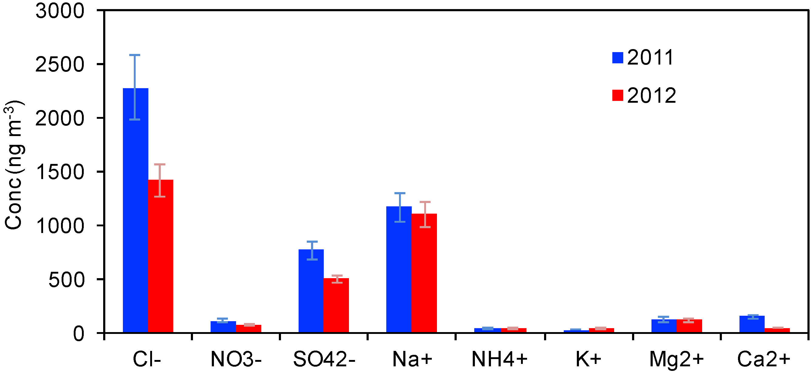
| Cl− | 1851 | 716 | 239 | 23 |
| Na+ | 1138 | 348 | 161 | 14 |
| SO42- | 637 | 199 | 110 | 7 |
| NO3− | 95 | 40 | 32 | 3 |
| NH4+ | 47 | 32 | 24 | 2 |
| K+ | 42 | 14 | 7 | 1 |
| Mg2+ | 125 | 47 | 18 | 1 |
| Ca2+ | 105 | 37 | 13 | 1 |
| OM | 1948 | 255 | 621 | 13 |
| EC | 30 | 2 | - - | - - |
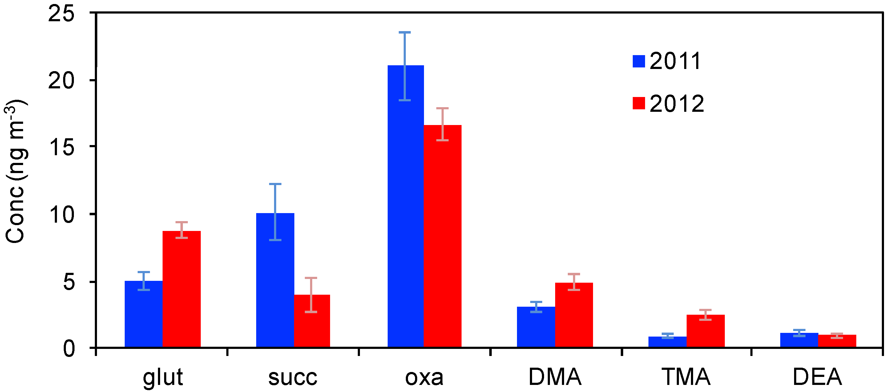
| glut * | 7 | 2 | - - | - - |
| succ * | 7 | 5 | - - | - - |
| oxa * | 19 | 6 | 5 | 1 |
| DMA * | 4 | 1 | - - | - - |
| TMA * | 2 | 1 | - - | - - |
| DEA * | 1 | 1 | - - | - - |
© 2019 by the authors. Licensee MDPI, Basel, Switzerland. This article is an open access article distributed under the terms and conditions of the Creative Commons Attribution (CC BY) license (http://creativecommons.org/licenses/by/4.0/).
Share and Cite
Ferrero, L.; Sangiorgi, G.; Perrone, M.G.; Rizzi, C.; Cataldi, M.; Markuszewski, P.; Pakszys, P.; Makuch, P.; Petelski, T.; Becagli, S.; et al. Chemical Composition of Aerosol over the Arctic Ocean from Summer ARctic EXpedition (AREX) 2011–2012 Cruises: Ions, Amines, Elemental Carbon, Organic Matter, Polycyclic Aromatic Hydrocarbons, n-Alkanes, Metals, and Rare Earth Elements. Atmosphere 2019, 10, 54. https://doi.org/10.3390/atmos10020054
Ferrero L, Sangiorgi G, Perrone MG, Rizzi C, Cataldi M, Markuszewski P, Pakszys P, Makuch P, Petelski T, Becagli S, et al. Chemical Composition of Aerosol over the Arctic Ocean from Summer ARctic EXpedition (AREX) 2011–2012 Cruises: Ions, Amines, Elemental Carbon, Organic Matter, Polycyclic Aromatic Hydrocarbons, n-Alkanes, Metals, and Rare Earth Elements. Atmosphere. 2019; 10(2):54. https://doi.org/10.3390/atmos10020054
Chicago/Turabian StyleFerrero, Luca, Giorgia Sangiorgi, Maria Grazia Perrone, Cristiana Rizzi, Marco Cataldi, Piotr Markuszewski, Paulina Pakszys, Przemysław Makuch, Tomasz Petelski, Silvia Becagli, and et al. 2019. "Chemical Composition of Aerosol over the Arctic Ocean from Summer ARctic EXpedition (AREX) 2011–2012 Cruises: Ions, Amines, Elemental Carbon, Organic Matter, Polycyclic Aromatic Hydrocarbons, n-Alkanes, Metals, and Rare Earth Elements" Atmosphere 10, no. 2: 54. https://doi.org/10.3390/atmos10020054