Arctic Sea Ice Decline in the 2010s: The Increasing Role of the Ocean—Air Heat Exchange in the Late Summer

Abstract

This study is focused on the specific features of ocean–air interaction in the Laptev Sea, in the late summer, on the basis of recurrent measurements during four expeditions in the 2000s and 2010s, atmospheric reanalysis products, and satellite ice concentration data. It was established that in the “icy” years, the accumulation of heat in the upper ocean layer is insignificant for the subsequent ice formation. In the “ice-free” years, the accumulated heat storage in the upper mixed layer depends on the duration of open water and the distance of the point of interest to the nearest ice edge. In a broader context, we considered possible links between the average ice area/extent in the August–September–October (ASO) period, and in the December–January–February (DJF) period, for two representative Arctic regions; that is, the Eurasian segment, defined within the bounds 60–120° E, 65–80° N, and the American segment, defined within the bounds 150° E–150° W, 65–80° N. Significant “seasonal memory”, characterized by the consistent change of the ice cover parameters in sequential seasons, was revealed in the Eurasian segment between 2007 and 2017. No linkage on a seasonal time scale was found in the American segment. A possible explanation for the distinguished contrast between the two geographical regions is proposed.

1. Introduction

The steady poleward advance of the open water area at the end of summer is in line with the existing climatic projections of the progressive transition to seasonal ice cover in the Arctic Ocean by the end of the 21st century [1]. The year 2007 could be considered as a sort of tipping point between the prevailing multiyear and seasonal sea ice in the Siberian Arctic seas [2]. Hydrometeorological processes in the seasonally ice-covered seas substantially differ from the seas under permanent ice cover, because of the enhanced heat exchange between the atmosphere and the upper water layer, a distinct freeze–thaw cycle, and a deeper penetration of various types of mixing.

There is growing evidence that a new state of the hydrographic regime is currently shaping under the rapidly changing conditions at the ocean surface in the East Atlantic sector of the Arctic Ocean [3,4,5,6]. It is expected that this new state will be characterized by warmer and saltier well-mixed upper ocean layers, instead of a quasi-two-layer structure with a cold and fresh upper layer under the permanent ice cover. A general north-eastward shift of such structural changes has already been documented in the Barents Sea and the Western Nansen Basin, where the main driver of change is the warm Atlantic Water (AW) inflow, where its influence on the upper ocean has intensified due to the reduction of ice cover [3,5]. Further to the east, the warm AW becomes sheltered from the ocean surface by high gradient transient layers, thereby losing an efficient means of delivering heat and salt upwards. In these regions, the possible driver of change is the excessive absorption of short-wave solar radiation under the conditions of increased duration of open water in summer. Whether this accumulated extra heat is rapidly lost to the atmosphere during the next fall, or the “memory” regarding the warmer surface layer is transferred to the first year ice properties, as suggested by [7], depends on multiple factors. The extended size of the ice-free area facilitates massive ice growth as soon as the surface water temperature reaches the freezing point. On the other hand, a longer duration of ice-free areas delays the onset of freezing, since more atmospheric heat can be accumulated in the upper mixed layer (UML). The rate of heat absorption depends on the prevailing atmospheric circulation patterns and the local weather conditions. Downward propagation of the absorbed heat in the water column, which ultimately determines the total heat content of the upper ocean at the end of the warm season, is controlled by density stratification and atmospheric dynamical forcing [8]. This heat has to be released to the air before the freezing can start. The rate of the UML cooling in the fall primarily depends on turbulent heat flux at the ocean-air interface, because during the polar night, radiation balance is permanently negative.

In this study, we validated the outlined theoretical considerations using field measurements and atmospheric reanalysis products. We focused our investigation on the central Laptev Sea, where recurrent hydrological transects and accompanying meteorological measurements were carried out in September 2003, 2005, 2013, and 2015, as a part of the ongoing NABOS (Nansen and Amundsen Basins Observations System, http://nabos.iarc.uaf.edu) research program.

The paper contains four sections, including the current one. In Section 2, we describe the data and methodology used. Section 3 is devoted to the joint analysis of the available data in the context of the basic ideas formulated above. In the discussion, we extend an outcome of the performed analysis for the tentative explanation of the interannual variability in the sea ice properties in the representative regions of the Arctic Ocean, observed during the 2000–2010s. General conclusions are formulated in the final section. Supporting information on the observational and data processing techniques, as well as the comparison between the in-situ observations and reanalysis data, is presented in the Appendix.

2. Data and Methods

Field data used in this study were collected during four research expeditions to the Arctic Ocean, carried out in August-September onboard the icebreaker “Kapitan Dranitsyn” (2003 and 2005), and the research vessels “Akademik Fedorov” (2013) and “Akademik Tryoshnikov” (2015). The scope of the investigations included multidisciplinary studies of the physical, chemical, and biological conditions in the Eurasian Arctic, with the major focus on the deep part of the Laptev Sea (see NABOS cruise reports at http://nabos.iarc.uaf.edu/). Hydrographic measurements were carried out at the cross-slope sections using the SeaBird-911plus CTD (Conductivity Temperature Depth) device (https://www.seabird.com/profiling/sbe-911plus-ctd/family?productCategoryId=54627473769, manufactured by SeaBird Scientific, USA). CTD accuracy is ±0.001 °C for temperature, ±0.0003 S/m for conductivity, and ±0.001 PSU for salinity. We used the vertical gradient of the potential density 0.01 kg∙m³∙m⁻¹ as the quantitative criterion for determination of the UML depth.

Atmospheric and sea ice data used in this study included the ERA-Interim reanalysis from ECMWF (European Centre for Medium-Range Weather Forecasts). [9] and the DMSP (Defense Meteorological Satellite Platform) digitized passive microwave satellite images [10]. These products are freely available on the internet. The ERA-Interim reanalysis is one of the most popular global datasets for climate studies, especially for data-sparse regions. For the Arctic region it is still not perfect [11], but it provides the best verification results for wind speed, near-surface temperature, and radiative fluxes in comparison to six other global reanalysis products, as is shown in a detailed evaluation study [12].

One of the key analyzed variables in our study is the total heat balance for the ocean surface, $B$, and its components:

$$B=Q_S+Q_L+F$$

(1)

where $Q_S$ and $Q_L$ are the net shortwave and longwave radiation, and $F$ is a total turbulent heat flux. Since, in our study, the turbulent heat exchange at the ocean-atmosphere interface is considered relative to the ocean, the positive$F$ values indicate heat transfer from the atmosphere to the ocean:

$$F=-\left(H+LE\right)$$

(2)

where $H$ and $LE$ are, respectively, the sensible and latent turbulent heat fluxes, which are directed from the ocean to the atmosphere according to their classic definition in atmospheric sciences. The methods of calculation of the turbulent fluxes according to in-situ ship-based observations are presented in the Appendix.

During the research cruises, meteorological measurements were permanently conducted on the route. The list of instruments used and the measured parameters is presented in the Appendix,

Table A1. The list of instruments used and the measured parameters during the 2013 and 2015 cruises.

Observed Parameter	Measurement Instrument
	NABOS-2013	NABOS-2015
Fluctuations of air temperature and three components of wind speed	Acoustic three-component anemometer Gill Wind Master, installed at the foredeck, 10 Hz frequency	Acoustic three-component anemometer METEK Sonic-3 Scientific, installed at the foredeck, 10 Hz frequency
Upward and downward fluxes of the shortwave and longwave radiation	Instrument cluster Kipp & Zonen (two pyrgeometers CGR-3 and two pyranometers CMP-21), installed at the crossbar on the upper deck, 1 min frequency
Meteorological parameters (temperature, pressure, humidity, wind speed)	(1) Aanderaa AWS2700 automatic weather station (spaced apart left and right shipboards), 1 min frequency (2) Ship weather station	(1) Marine automatic weather station Airmar WX150 with an internal GPS, compass, inclinometer, and accelerometers, installed at the foredeck, 1 Hz frequency (2) Ship weather station
Characteristics of ship movement (speed, location, inclination)	Three-axis accelerometer ADXL330, inclinometer, GPS-receiver of Garmin 17N standard
Sea surface temperature	Infrared radiometer HEITRONICS KT19.82, 1 Hz frequency
Air temperature profile in the lower troposphere	Microwave temperature profiler MTP-5, installed at the upper deck at a height of 25 m above sea level, 5 min frequency, vertical resolution 50 m
	Vertical range 0–600	Vertical range 0–1000

. In 2013 and 2015, all components of heat balance at the sea surface were calculated from the shipborne measurements. In 2005, the radiation balance was reconstructed from the ERA-Interim reanalysis data. In 2003, all components of heat balance were reconstructed from the ERA-Interim reanalysis data. For consistency, we based the analysis of meteorological conditions on ERA-Interim products in all four years. The quality of the reanalysis data was confirmed by comparison to shipborne measurements in 2005, 2013, and 2015 (see Figure A5 in the Appendix). In cases where the discrepancy between the shipborne measurements and the ERA-Interim data appeared to be too large, we based our conclusions on the shipborne measurements, considering them to be more reliable.

3. Ice and Hydrometeorological Conditions in the Central Laptev Sea in Summer

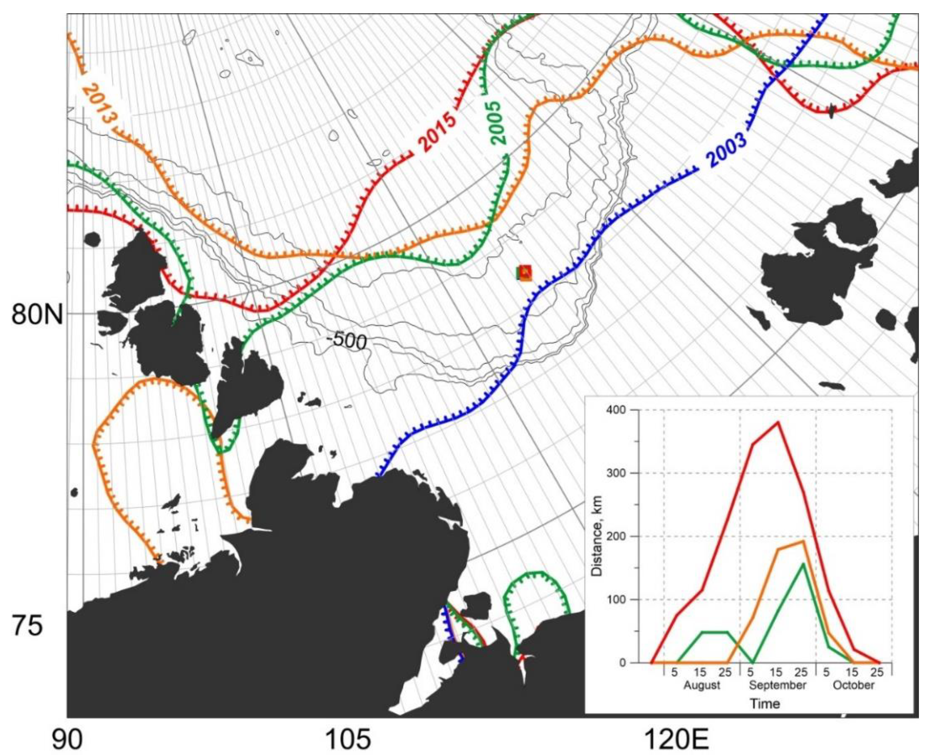
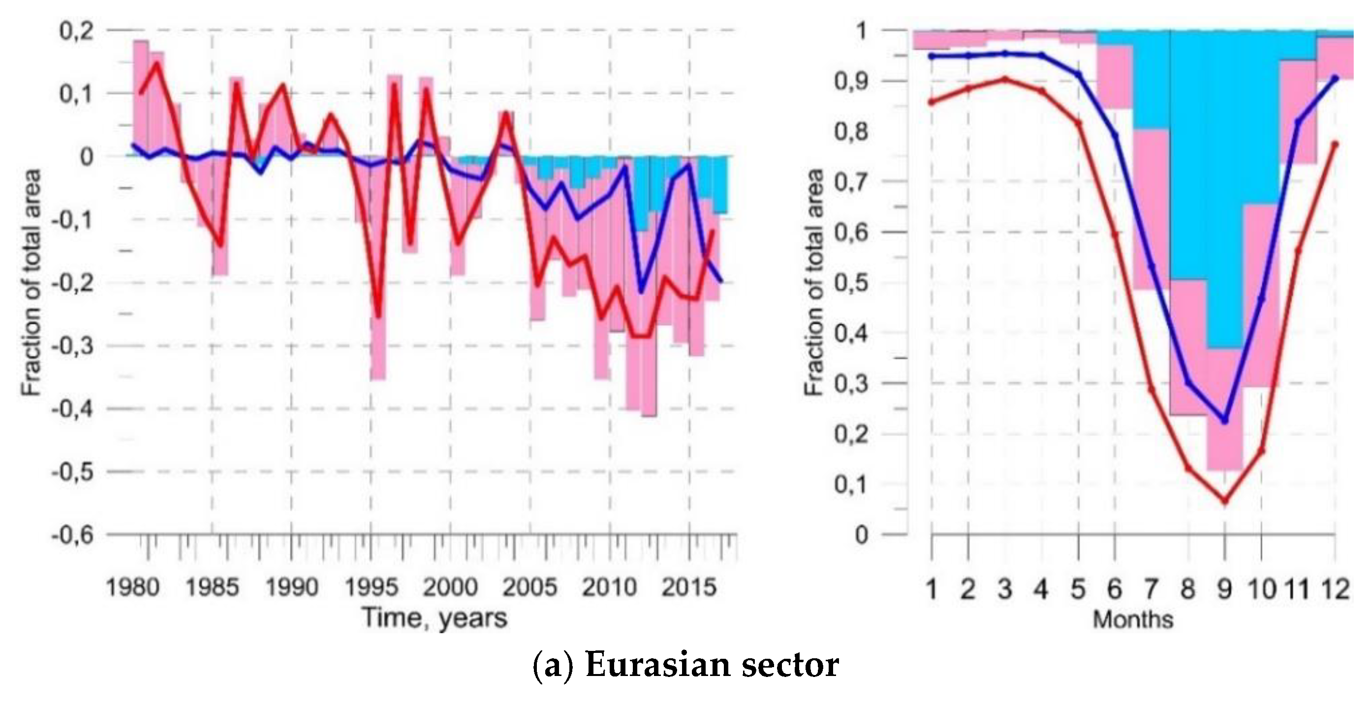
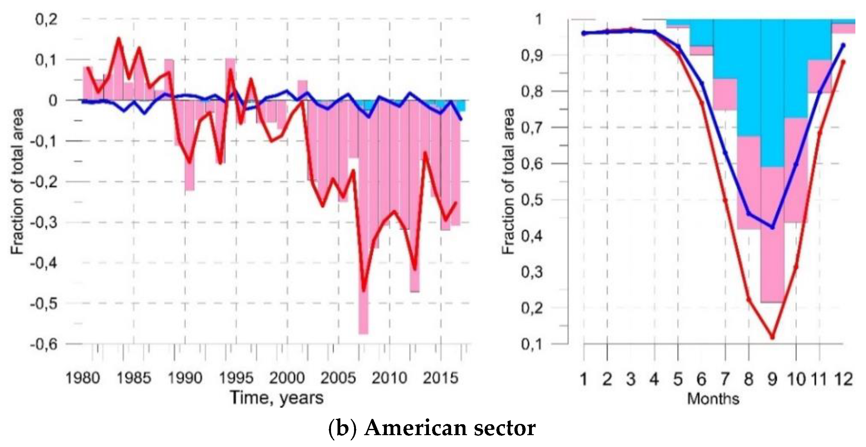
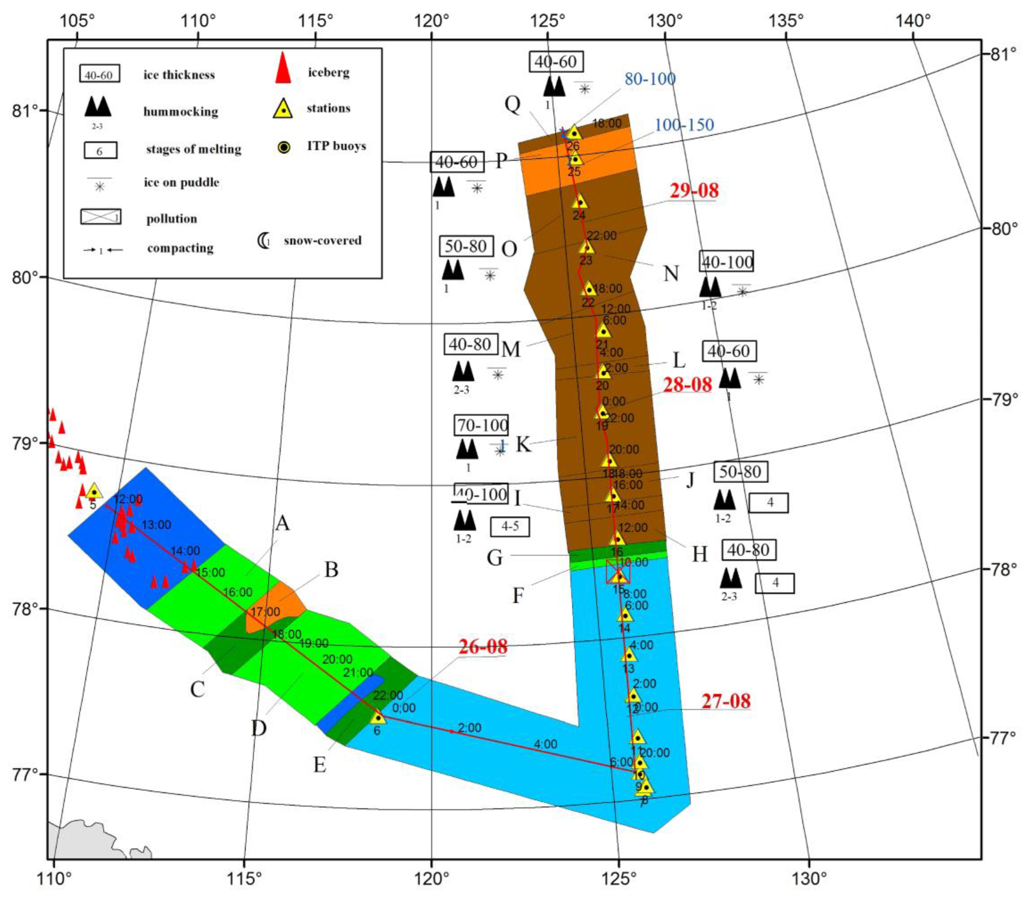
Sea ice extent (the edge of the ice concentration exceeding 15%) at the peak of the summer minimum is the conventional indicator of interannual changes in the state of the Arctic sea ice cover. This indicator, however, does not consider ice thickness (age). In this sense, the four considered years belonged to different ice regimes in the Laptev Sea, that is, the dominance of perennial ice up to 2005 and the substantially increased fraction of seasonal ice in 2006 and after (see details in Discussion section). The mean September sea ice extent in the Laptev Sea according to the DMSP satellite data for four studied years is presented in Figure 1. The position of the recurrent CTD stations is shown by colored squares. Supportive additional information is given in the inset and in

Table 1. Description of the recurrent conductivity temperature depth (CTD) stations. The dates of opening or closing signify the first date when the CTD station was outside or inside the border of 15% ice concentration. The mean distance to the ice edge is the nearest linear path to the border of 15% ice concentration in any direction.

Year	Date-1	Date-2	Lat., °	Long., °	Date of Opening, ±5 Days	Date of Closing, ±5 Days	Duration of Open Water, ±10 Days	Mean Distance to the Ice Edge, km
2003	01.09	06.09	78.445	125.662	n/a	n/a	n/a	n/a
2005	14.09	20.09	78.464	125.668	25.08	05.10	40	60
2013	27.08	07.09	78.395	125.785	30.08	05.10	35	122
2015	02.09	19.09	78.460	125.930	30.07	20.10	80	193

.

3.1. Ice Conditions

A general northward shift of the ice edge is clearly seen from the 2000s to 2010s (about 300 km between 2003 and 2015). However, the difference between 2005 and 2013 is rather small, pointing out the significant year-to-year variations. In 2003, the position of the recurrent CTD station was permanently in the ice covered waters, while in the other years, the position was in the open water for different periods of time (see the inset in Figure 1). In 2005, the open water first reached the point of interest on August 25 ± 5 days. However, for the next 20 days, the distance to the ice edge did not exceed 50 km. Considering the 10 day averaging of the used DMSP product and the relatively large error of edge determination in the melting season [13], we may expect that in 2005, between August 15 and September 15, the point was very close to, or even within, the marginal ice zone (MIZ). Visual observations along the ship track during the 2005 NABOS cruise confirmed the existence of steady open water in the area of the recurrent CTD station after September 14 (www.nabos.php), which corroborates the DMSP product results. In 2013 and 2015, the position was in the open water and it was far away from the nearest ice edge for a longer time period. Maximum duration of open water was observed in 2015: 80 ± 10 days, i.e., almost three months. In 2013, the total duration of open water was even shorter than in 2005, but the mean distance to the ice edge was two times larger. A comparison of the ice edge position from the DMSP product to the visual observations along the ship track (see Figure A1 in the Appendix) allowed us to conclude that in 2013, the point was already in the open water during the first CTD cast on August 27.

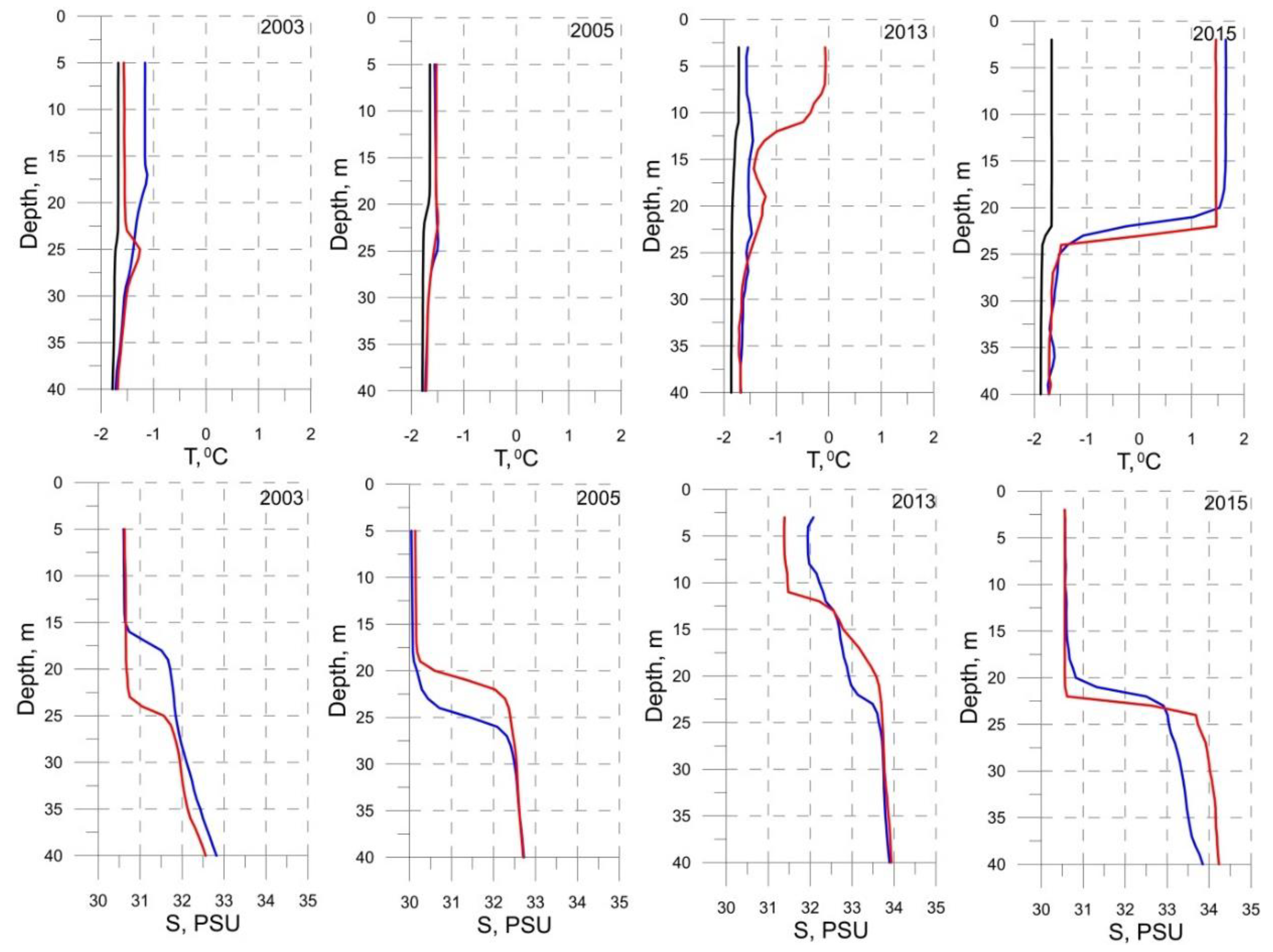
3.2. Hydrographic Conditions

The background thermohaline structure in the upper ocean in September, during four considered years, was primarily controlled by the ice conditions. This expected linkage is illustrated by the temperature and salinity profiles in the upper 40 m depth layer at the recurrent CTD stations in Figure 2. In 2003 and in 2005, water temperature in the entire 40-m layer was negative and did not exceed −1 °C. In 2003, the maximal departure from the freezing point, up to 0.5 °C, was observed at the base of the UML. In 2005, the maximal departure was less than 0.25 °C. On the contrary, in 2013 and 2015, the departure from the freezing point in the UML exceeded 1 degree during the second CTD cast, reaching 3 degrees in 2015. However, on the 5–14 day time scale, which corresponds to the time interval between recurrent CTD casts, the effect of ice conditions on the vertical structure was less unequivocal. For example, the evolution of the UML demonstrated definite similarities in specific years with contrasting ice conditions. In “icy” 2003 and in “ice-free” 2015, the thickness and salinity of the UML increased unidirectionally between the two recurrent CTD casts, reaching about the same value of 23 m during the second cast. In 2005, the UML was 4 m shallower during the second cast. In 2013, there was no distinct seasonal UML during the first cast at all, while at the second cast, it appeared within the 11 m depth. Temperature change in the UML between the two casts in the neighboring “ice-free” years was opposite—an increase in 2013 and a decrease in 2015, while corresponding salinity changes were unidirectional (increase) in both years. These similarities and differences in the observed short-term changes over the years, which were characterized by different and similar ice conditions, point to variable atmospheric forcing as a probable factor affecting the state of the upper ocean layer in the warm season.

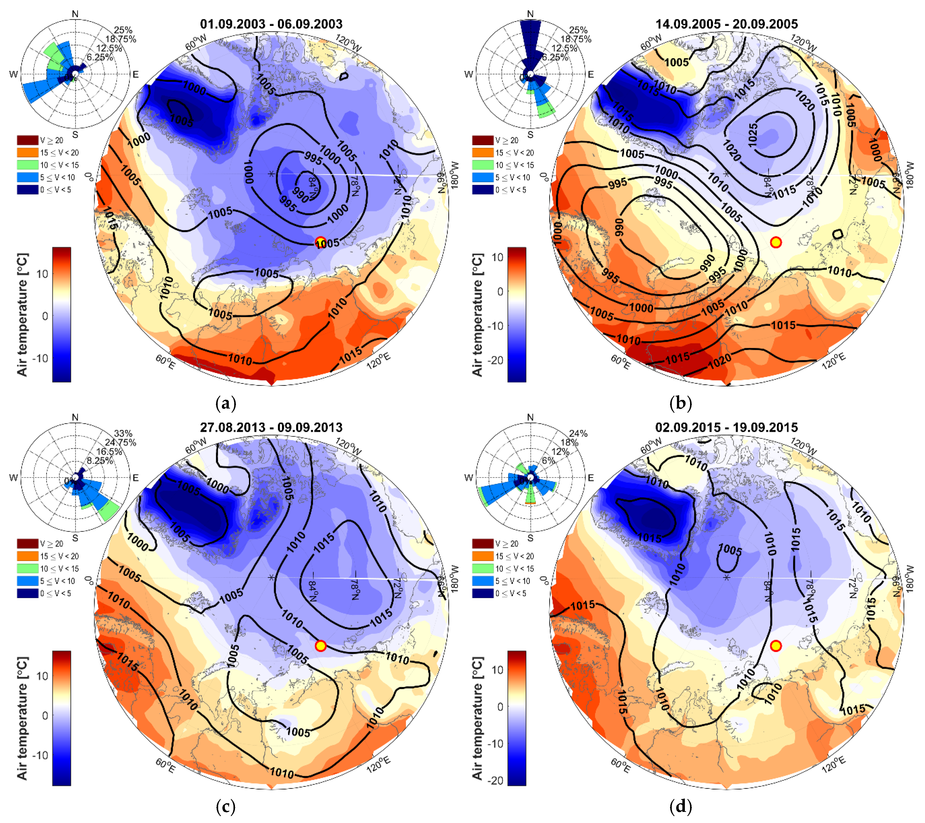
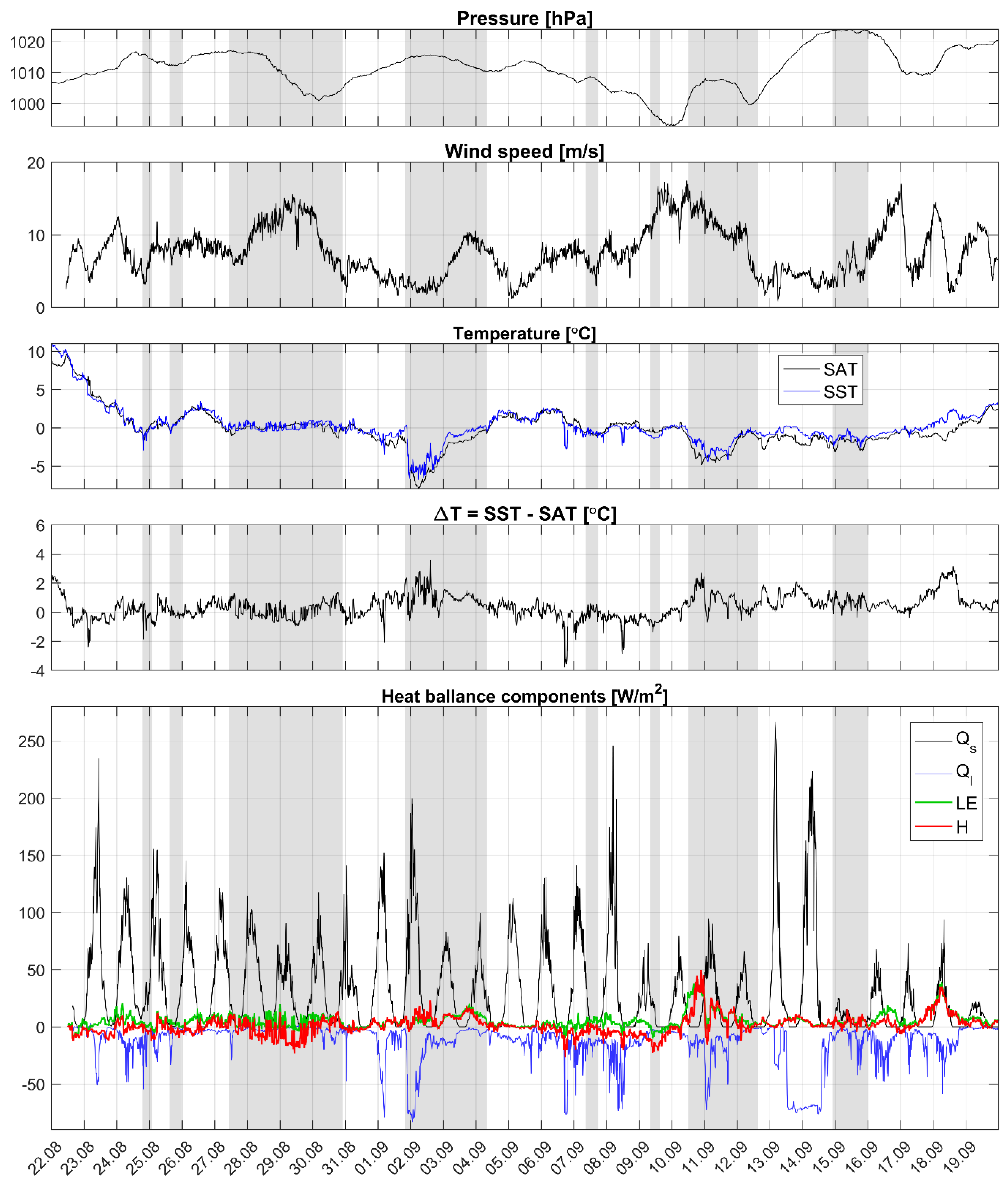
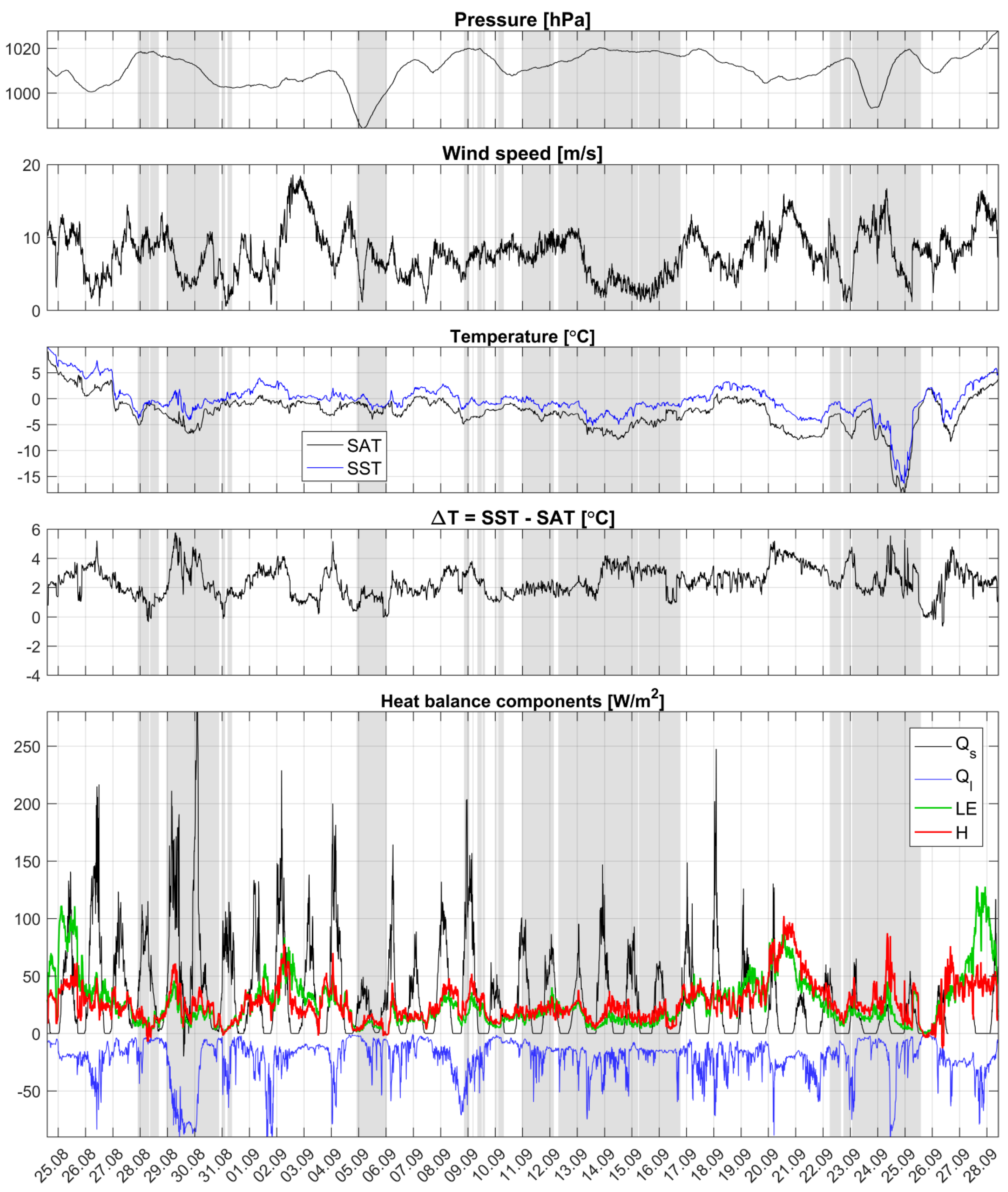
3.3. Weather Conditions

Synoptic scale atmospheric forcing at the ocean surface is determined by weather conditions. The distinctive feature of the Siberian shelf seas in general (and the Laptev Sea in particular) in summer is a close neighborhood (on the scale of the baric systems) of cold ice covered surfaces, a warm continent, and relatively warm open water in between. Hence, the intensity of the ocean–air energy exchange, and even its sign, primarily depends on the characteristics of the air masses that enter the affected area. This feature is a principal difference between the Polar regions and the lower latitudes. In the mid-latitudes, there is a distinct division between the summer season, when the colder ocean gains heat from the warmer air, and the fall-winter season, when the warmer ocean releases heat to the atmosphere. In the Polar regions, even in the mid-summer season, the upper ocean layer may act as a heat absorber, as well as a heat emitter, because of the near-zero sea surface temperature (SST) close to the ice edge under the ice-free conditions [14]. An air flow, which floods over an ice-free surface, may be either warmer, if originated over the continent, or colder, when coming from the ice covered regions in the high-latitude Arctic.

Considering these possible options, we assessed the synoptic conditions over the four considered years according to the ERA-Interim reanalysis data. In 2003, the position of the recurrent CTD station was permanently at the periphery of the vast cyclone occupying almost the entire Arctic Ocean (Figure 3a). Western winds forced the ice edge to the east, keeping the point in the MIZ. In 2005, between September 14 and 20, the central Laptev Sea was located in a saddle-shaped sea level pressure (SLP) field between four large scale pressure systems, centered over the Arctic Ocean and the adjacent continent (Figure 3b). Weak SLP gradients caused intermittent winds and the slow transport of air masses. Within the entire time interval between the two recurrent CTD stations in 2013, the study area remained in the pathway of warm air flow from the continent between the anticyclone over the central Arctic Ocean, and the cyclone, centered in the Kara Sea (Figure 3c). The time interval between the recurrent CTD stations in 2015 was the longest compared to the other years, that is, two and a half weeks. The study area was mainly in the cyclonic circulation field. This caused the prevalence of western winds from the Kara Sea and an inflow of the air with near-zero °C surface air temperature (SAT) (Figure 3d).

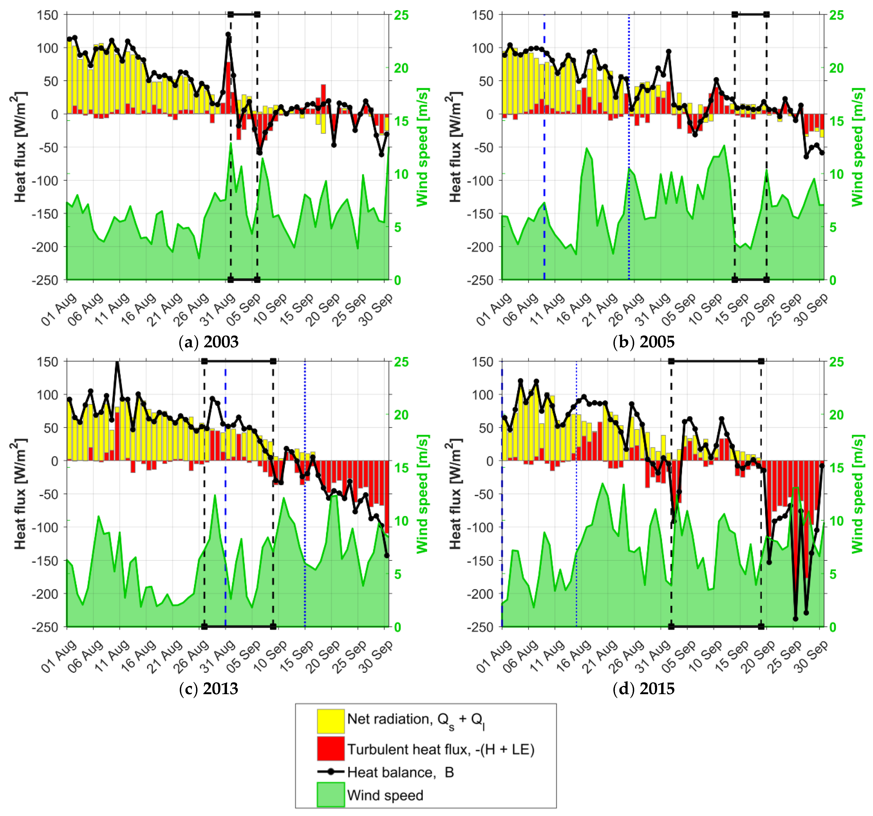
3.4. Ocean–Air Energy Exchange

Time series of total heat balance at the area of the recurrent CTD station through August–September from the ERA-Interim data (daily average values) are shown in Figure 4 (in the figure, and hereafter in the text, we consider the total turbulent heat flux $F$, where positive values indicate a heat transfer from the atmosphere to the ocean. See Equations (1) and (2). Time series of the specific components of total heat balance along the ship route are presented in the Appendix, Figure A5. A common feature for all four years was the gradual decrease of radiation balance from the highest values (up to 100 W/m²) in early August to near-zero values at the end of September (Figure 4). Such a consistent pattern is obviously explained by the seasonal cycle of the short-wave radiation. Small-scale variations of radiation balance, superimposed on this general seasonal pattern, might be linked to variable cloudiness and the difference in long-wave radiation flux at the ice-free and ice covered underlying surface.

On the other hand, the difference in the pattern of turbulent heat fluxes between 2003, 2005, 2013, and 2015 for the entire two-month time interval was very visible. In 2003 and in 2005, turbulent heat fluxes were alternating around zero until the end of September. In 2013 and in 2015, intensive ocean heat losses due to turbulent exchange were observed during the entire second part of September (mean values of the total turbulent heat flux $F$ over the period from September 15 to September 30 at the recurrent CTD site were −49 W/m² on average in 2013 and −82 W/m² in 2015, according to the ERA-Interim reanalysis), thus making the total heat balance at the surface substantially negative.

However, there was a large difference in the turbulent heat balance at the smaller time scale in 2013 and 2015. In 2013, the mean total heat balance between the two recurrent CTD casts was positive. Both data sets (direct measurements and ERA-Interim reanalysis) consensually pointed out that the main contributors to the total heat balance in 2013 were radiation components. In 2015, the turbulent heat flux patterns between the two recurrent CTD casts were more ambiguous. According to the ERA-Interim reanalysis, the negative and positive heat fluxes alternated, yielding a small average total heat flux (Figure 4d). On the other hand, direct measurements indicated a constantly negative total heat flux along the ship route with the dominance of the turbulent heat flux (Figure A5c). Hence, in 2015, we preferred to trust the shipborne measurements and cautiously concluded the decisive contribution of turbulent fluxes to the total heat balance.

Turbulent heat fluxes are controlled by the state of the underlying surface (ice of various type or an open water), the weather conditions (SAT and wind speed), and the SAT–SST difference. A closer look at the time series of the observed meteorological parameters (see the Appendix, Figure A2, Figure A3 and Figure A5) confirmed our conclusions on the dominance of turbulent heat fluxes in the total heat balance of the ocean surface in 2015. In 2013, the SAT was more than 2 °C lower than that in 2015, according to ship-based measurements, while the observed SST values in the two years were practically similar (see

Table 2. Mean values of the observed surface air temperature (SAT), sea surface temperature (SST), and their difference ΔT, averaged over the whole cruise track in the Laptev sea region (100–150 °E) for the 2013 and 2015 cruises.

Region of Averaging	Year	SAT	SST	ΔT = SST − SAT
Average over ice-free water along the whole cruise tracks	2013	0.68	1.03	0.34
	2015	−1.33	1.08	2.41
Average over ice-free water in Laptev sea region (100–150 °E)	2013	0.35	0.43	0.08
	2015	−2.14	0.41	2.55

for details). Hence, the observed SAT–SST difference in the Laptev sea was close to zero in 2013 and −2.5 °C in 2015. Warmer air flow from the continent in 2013 resulted in a near-zero turbulent heat flux. In 2015, the relatively cold air inflow on the warmer (over 2 °C) ice-free surface provided negative turbulent heat fluxes. This resulted in generally negative heat balances at the ocean–air interface between the two recurrent CTD casts in 2015, instead of the positive heat balance in 2013.

3.5. Heat Accumulation in the UML

In this subsection, we consider the evolution of the heat storage in the UML according to the recurrent CTD casts with linkages to the atmospheric forcing and ice conditions. The heat storage $C$ is defined relative to the freezing point temperature:

$$C=\rho c_{p}h\left(T-T_f\left(\mathrm{S}\right)\right)$$

(3)

where $\rho$ is the water density, $c_p$ is the water heat capacity, $h$ is the UML depth, $T$ is the mean temperature of the UML, and $T_f$ is the freezing temperature that depends on the salinity$\mathrm{S}$.

Long duration of open water is the prerequisite condition for building up heat storage in the UML. In 2003, the studied area was permanently covered by pack ice of variable concentrations. Despite similar radiation balance values, as in the other years (see Figure 4), the temperature in the UML (15 m thick during the first CTD cast, see Figure 2 for all the discussed casts) was −1.16 °C. Five days later, it decreased by the ΔT = 0.4 °C, almost reaching the freezing point, and the UML deepened to 23 m. The mean salinity decrease (ΔS) in the upper 19–20 m was equal to 0.15 PSU, from 30.79 ÷ 30.82 to 30.65 PSU. These unidirectional changes of thermohaline parameters point out that incoming atmospheric heat was spent on ice melt. A simple calculation based on Equation (2) in Reference [15]:

$$\Delta S=S(1-\frac{67}{67+\gamma \Delta T})$$

(4)

where γ = ρ_i/ρ is the relation of mean ice and sea water densities that the temperature decrease due to ice melt by −0.4 °C, within the 23-m thick layer, led to a salinity decrease by −0.16 PSU, provided that the layer was well mixed. The latter was likely to be the case due to stormy conditions experienced from September 1–3, 2003 (see Figure 4a), which provided intensive turbulent mixing. Equation (1) for the UML depth $h$ in Reference [15],

$$h=\frac{67\Delta h_i}{\Delta T}$$

(5)

gives that temperature and salinity decrease corresponds to 10 cm of ice melt ($\Delta h_i$). Taking into account that 6 cm of ice melt may be due to the atmospheric heat flux only (26 W/m², the average heat balance value between September 1 and 5, see Figure 4a), this amount appears reasonable because of the additional bottom and side melt. Hence, we may conclude that under the icy conditions in 2003, by the end of the summer season, the heat storage in the upper layer remained small (7.4 MJ/m²), since the incoming atmospheric heat was almost totally spent on the ice melt.

However, the presence of open water does not guarantee a noticeable warming in the UML. In 2005, the recurrent CTD station was intermittently in the open water or in the MIZ 30 days prior to the first CTD cast. It is important to note that at the time of the first cast (September 14), the ice edge moved south reaching that point. Proximity to the ice edge probably determined the lack of warming in the UML in August and in the first half of September, despite the high positive heat flux (39 W/m² on average between August 15 and September 14). Another explanation is that the export of ice from the north in mid-September caused the rapid cooling of the UML due to the local ice melt. This option is less probable, because there was virtually neither a temperature change (−1.56 °C) in the UML, nor a substantial change in its thickness (−3 m) between the two casts. The salinity increase in the UML during this time interval (+0.09 PSU) additionally points out that there was no ice melt. This slight salinity increase may have been attributed to an entrainment of cold halocline waters in the UML, which did not change the temperature. Heat flux at the ocean surface between the two recurrent CTD casts was small (11 W/m² on the average, see Figure 4b), thereby resulting in the preservation of nearly the same heat content in the UML (7.4 MJ/m²) as during “icy” 2003, despite the relatively long duration of open water.

Build-up of the UML heat content in the absence of sea ice could be revealed from the two recurrent CTD casts in 2013 and 2015. Vertical temperature profiles on August 27, 2013, essentially rendered the profiles in icy 2003 and 2005. Down to the 40 m depth, the temperature was quasi-uniform and close to the freezing point. Salinity contrast between the surface and the 40 m depth was less than 2 PSU. A sort of halocline between 8 and 22 m was split into several segments with small and variable vertical gradients. Hence, we could anticipate that the vertical thermohaline structure during the first CTD cast in 2013 represented an initial state of the upper ocean water column after the ice cover had just disappeared. The latter was in line with the satellite ice maps and cruise observations. During the next 11 days, a well-defined UML embedded by sharp pycnocline had formed as a result of the heat uptake from the atmosphere and the turbulent mixing [8,16].

Average heat flux at the surface between August 27 and September 7 ($\Delta t$ = 11 days) was equal to 50 W/m². The temperature rise (ΔT) was calculated from the one-dimensional heat balance equation described in Reference [3]:

$$\Delta T=\frac{B·\Delta t}{\rho c_{p}h}$$

(6)

applied to $h=11\mathrm{m}$, the UML is equal to 1.28 °C, while the actual temperature increase was 1.04 °C (c_p denotes the specific heat of sea water at a constant pressure). Additional warming in the UML could be attributed to the horizontal mixing with surrounding waters. As a result of the heat uptake, by September 9, the UML temperature reached a temperature of −0.26 °C (1.46 °C above the freezing point). The heat content by this date reached 65.8 MJ/m², which was an order of magnitude higher than in 2003 and in 2005.

In 2015, the first CTD cast was done on September 2, when the warming season was coming to an end. Therefore, the vertical structure of the upper ocean layer represented the state after the peak of warming had already passed, under conditions when open water existed for about one month. Very sharp pycnocline, between 19 and 26 m, separated the warm and fresh UML from the cold and saline waters below. The UML temperature equaled 1.61°C, corresponding to a 3.29 °C departure from the freezing point. After 17 days (on September 19), the pycnocline upper boundary deepened to 22 m, while the lower boundary remained at 26 m, thereby increasing the vertical gradients of the properties. Despite a weak positive average heat flux at the ocean surface (10 W/m² according to the ERA-Interim data), the temperature of the UML decreased by 0.15 °C, reaching 1.46 °C. As was mentioned before, in 2015, the ERA-Interim data substantially contrasted with the direct measurements, which showed a total negative heat balance due to the dominance of turbulent fluxes. The latter was in line with the observed temperature decrease in the UML. The heat content of the UML on September 19 equaled to 282.3 MJ/m², which was four times larger than in 2013.

4. Discussion

In this study, we focused on the specific features of the ocean-air interaction in the Laptev Sea during summer, on the basis of recurrent measurements during four expeditions in 2003, 2005, 2013, and 2015. The transition to an increasingly seasonal sea ice regime after 2007 draws a distinct timeline between contrasting ice conditions before and after this year, thereby allowing the assessment of possible changes in the ocean-air interaction processes caused by this transition.

Our main goal was to assess the relative significance of various factors in the buildup of heat content of the upper ocean layer at the doorstep of the next cold season. In a general sense, the increased duration of open water in the summer provides the prerequisite conditions for heat absorption in the upper ocean layer. However, the positive radiation balance in the high Arctic culminates in the middle of the astronomical summer, while the peak of the open water area typically occurs in the first half of September. By that time, the shortwave radiation flux is declining and a turbulent heat exchange may dominate the total heat balance at the ocean surface. Thus, the rate of removal of the heat absorbed in the upper ocean layer during the fall primarily depends on the atmospheric circulation patterns and the relation of these patterns to weather conditions. Assuming an average rate of heat loss through the fall in the range 100–200 W/m², we required less than a day for the UML temperature to reach the freezing point in 2003 and 2005, then from 3 to 6 days in 2013, and from 16 to 32 days in 2015. The latter meant the visible delay of the freezing onset in 2015. The 15 day delay of ice emergence (compared to 2005 and 2013) was captured by satellite imagery in 2015 (see Figure 1-inset). However, it is impossible to detect whether the first ice at this site was formed locally or was imported from the north. A crude estimation of the possible effects of a delayed freeze onset on the seasonal ice thickness may be applied using the empirical formula described in [17]:

$$h^2+50h-8{{\displaystyle \int }}_0^{\tau }|T_{-}\left(t\right)|dt=0,$$

(7)

where h is the ice thickness, T₋ is the air temperature below zero, and τ is the time interval of calculation. Although this equation was derived for the fast ice in the Laptev Sea, it is applicable for the estimation of ice growth in the open ocean, provided that oceanic heat flux is absent.

Taking the average winter SAT in the Laptev Sea as equal to −30 °C [18], we obtain the thickness of the one-year ice after 180 days of ice growth, equal to 182 cm. Reduction of the time interval by 16–32 days gave an 8–17 cm reduction in the one-year ice thickness. Although this value is rather small, it is detectable by direct measurements. Moreover, at the shorter time intervals, the relative thinning of ice is substantially greater, which may have an effect on the ice cover properties in mid-winter, as discussed below.

The obtained results may be cautiously extended on a larger scale. Taking into account the non-uniform spatial distribution of sea ice cover at the peak of summer, at a minimum we consider two specific segments around the Arctic. We define the ‘Eurasian’ segment within the bounds 60–120° E, and the ‘American’ segment within the bounds 150° E–150° W. The southern and northern boundaries of both segments were defined at 65° N and 80° N, respectively. The western margin of the Eurasian segment was chosen as 60° E to exclude the Western Nansen Basin and the Barents Sea, being the regions directly affected by the warm Atlantic Water, where the substantial reduction of winter ice cover in the 2010s was well documented [3,5]. Longitudinal margins of the American segment were selected in order to cover the area where the record retreat of ice cover had occurred in 2007.

Time series of the mean anomalies of ice area and ice extent, that is, the border of 15% ice concentration (shown as the fraction of the total area of the corresponding segment) during the August–September–October (ASO) period and the December–January–February (DJF) period, for selected segments, are shown in Figure 5. Anomalies were calculated relative to the mean values during the time interval 1980–2000 when the ice conditions were rather stable. The mean monthly values of both parameters for the time intervals 1980–2000 and 2007–2017 are also shown in the same graphs. A similar feature in both time series, for both segments, was the substantial increase of the ASO negative anomalies during the 2000–2010s. In the American segment, the shift to the milder ice regime started in 2003, while in the Eurasian segment, this began two years later. The maximal area of open water in the American segment was observed in 2007. In the Eurasian segment, the maximal ice decrease was observed in 2012. Comparing Figure 5 with Figure 1 in Reference [19], we argue that from 2012 onwards, the interannual variability of the ice extent in the Eurasian segment (probably together with the Barents Sea and the Western Nansen Basin, not considered here) notably shapes the pan-Arctic pattern of the interannual variability.

The DJF time series demonstrated a marked shift to the milder ice regime after 2005 in the Eurasian segment. In the American segment, there is no change from 2003 onwards compared to the span from 1980–2000. This was consistent with the pattern at the mean seasonal variability plots. The shift to the reduced values of both ice parameters in the winter months was very well pronounced in the Eurasian segment. In the American segment, there was no such shift at all—from January until April, the ice area and extent were the same in the two considered time intervals, despite the fact that the summer ice reduction in the Eurasian sector was only half that of the American segment. Hence, we could conclude that the “seasonal memory” between the ice cover properties in summer and in the following winter after 2005 was typical only for the Eurasian segment.

To understand the possible reasons behind the “Eurasian-American” difference, we considered the time series of the 3-month average (ASO) atmospheric circulation patterns over the Arctic, derived from the ERA-Interim reanalysis daily data. These patterns were presented by the spatial and temporal components of the anomaly of sea level pressure (SLP), which were determined using the standard algorithm for empirical orthogonal function decomposition (EOF). EOFs are used to distinguish the main patterns (for example, the SLP) and to indicate the prevailing localization of structures [20,21]. The EOFs are mathematically orthogonal and independent of each other. The first three EOFs describe 86% of the total variance (see Figure 6, left panels) and they are well separated.

The first EOF pattern (58% of the total variance) represents Arctic oscillation (AO) [22,23]. The positive phase of the AO (corresponded to EOF1) is associated with a negative SLP anomaly close to the North Pole. Almost the entire Arctic Ocean is covered by this circulation cell. However, Ogi et al. [24,25] emphasize that the summer AO pattern has a smaller meridional extension than the conventional AO. The second EOF pattern (17% of the total variance) forms a dipole containing two cells that are opposite in signs. The first zone is centered over the southern Kara Sea and it is a more compact cell, while the second zone is centered over the Canadian Basin. The former is stretched in the zonal direction, with the western periphery reaching the Norwegian Sea and the eastern periphery on the Laptev Sea shelf. The second EOF was previously detected as the Pacific/North American teleconnection pattern (PNA) [26]. The third EOF (11% of the total variance) is more meridional, has a highly asymmetric dipole field, and corresponds to the Arctic dipole (AD) [27,28,29]. A positive phase of the AD pattern is associated with a negative SLP anomaly on the North American side of the Arctic and a positive SLP anomaly on the Siberian side of the Arctic. However, the EOF’s size of area and boundaries can influence the EOF patterns [30]. EOF calculations for various sizes of areas were carried out in this study. It was shown that with a shortening of the zone, the key features of the first two EOFs remained the same (with a slight shift of maximum to the northeast); the third EOF changed significantly, where it formed a saddle pattern, the so called Buell patterns [30]. Time series of the corresponding principal components (PCs) are shown on the right panels of Figure 6. PC2 attracts particular attention due to the presence of a steady increasing trend after the absolute minimum in 2007. Two other significant PCs did not show any sort of persistent behavior at the decadal time intervals. The range of PC1 interannual oscillations was the largest during the 1980s–1990s (over four units), while after 2000 it reduced by two times. PC3 also did not show any notable trends. Similar to PC1, the range of PC3’s interannual variability substantially decreased at the end of the record (i.e., from 2010 onwards).

Our interpretation of these features in relation to the sea ice variability described above is as follows. Large scale cyclonic circulation over the Arctic Ocean (PC1) enforces a poleward drift of the ice in the American segment, but it slows down the ice export from the Siberian seas. At the same time, this cyclonic circulation maintains an inflow of air from the continent. The temperature of the continental air is warmer than the ice or water surface in the summer. In the fall, the temperature of the air, flowing in from the cooling continent, drops down, thereby favoring heat loss at the open water surface due to a turbulent heat exchange. In the Eurasian segment, a positive PC1 retards summer warming due to an inflow of the cold air from the ice-covered ocean north of Greenland. By the end of September–early October, this cooling effect might become weaker, because by that time, the sea surface in the northern Barents Sea has already been heated by the solar radiation and it warms up the incoming air from the central basin. Therefore, the anomalous reduction of the summer sea ice area and extent in the American segment, as well as the fast cooling at the ocean surface in the fall, may be explained (at least partly) by the large scale cyclonic circulation over the Arctic Ocean.

However, PC1 does not provide any clue to the explanation of the revealed “seasonal memory” between the sea ice properties during the ASO and DJF periods in the Eurasian segment. We argue that an increased contribution of PC2 after 2005, which turned from negative to highly positive values in recent years, was the major driver behind this “seasonal memory”. An elongated shape of the EOF2 anticyclonic cell ensured the pumping of warm and humid air from the ice-free Norwegian Sea and southern Barents Sea when the PC2 was positive. In the fall, this relatively warm air served as an “insulator” for the heat accumulated in the upper ocean during the summer, slowing down the UML cooling and delaying the onset of freezing. This insulating effect was obviously the strongest in the western part of the Eurasian segment. For example, in the fall of 2016, the anomalously high sea surface temperatures over the Barents-Kara Seas created an extremely low pan-Arctic sea ice extent throughout the fall and the early winter. In mid-November 2016, the sea ice extent even decreased for several days [31]. In the American segment, the effect of an enhanced PC2 was the opposite. Counterclockwise circulation over the Canadian Basin delivered cold air from the Greenland pack ice towards Alaska and the Bering Strait, leading to enhanced heat loss from the ocean surface to the atmosphere, facilitating faster ice formation.

5. Conclusions

The progressive reduction of Arctic sea ice cover alters the processes of ocean-air interaction. In the Arctic, ocean-air turbulent heat exchange is particularly significant in the late summer when the short wave radiation balance at the ocean surface is reduced, and the turbulent heat fluxes take over in the total heat balance. Local ice formation in the open water commences only after the sea surface temperature drops to the freezing point. The required time for the freezing onset depends on the amount of heat accumulated in the UML throughout the summer, as well as the rate of this heat removal. Joint analysis of the observations, atmospheric reanalysis products, and satellite data allowed for the assessment of the heat storage changes in the UML related to the variable atmospheric forcing under contrasting ice conditions in the Laptev Sea at the doorstep of the fall. It was established that in the “icy” years (2003 and 2005), the accumulation of heat in the UML was insignificant for the subsequent ice formation because the absorbed heat was mostly spent on the ice melt until the end of the summer. In the “ice-free” years (2013 and 2015), the ultimate heat storage in the UML depended on the duration of open water, the distance of the point of interest to the nearest ice edge, and on the synoptic weather patterns. We did not find any direct links between the UML heat content and the strength of the underlying pycnocline, although such links could be expected. In our opinion, the water column in the Laptev Sea has so far not undergone a significant structural transformation, similar, for instance, to the Western Nansen Basin [32]. Hence, the heat accumulation in summer was confined to the relatively shallow (up to 20–25m) surface layer. However, the heat capacity of this thin surface layer may be large enough to delay the onset of freezing by up to tens of days, depending on the rate of surface cooling during the fall.

In the format of discussion, we considered the possible links between the average ice area/extent in August–September–October (ASO) period, and in the December–January–February (DJF) period, for two representative Arctic regions, that is, the Eurasian segment, defined within the bounds 60–120° E, 65–80° N, and the American segment, defined within the bounds 150° E–150° W, 65–80° N. Significant “seasonal memory”, characterized by the consistent change of the ice cover parameters in sequential seasons, was retrieved in the Eurasian segment between 2007 and 2017. No linkage to the seasonal time scale was found for the American segment, despite an even stronger reduction of the ASO ice extent/area in this region from 2007 onwards. We explain the distinguished “Eurasian–American” contrast as being the result of the increasing (since 2007) intensity of a dipole circulation mode over the Arctic Ocean in the ASO period. This circulation mode is described by the second-in-order member of the Arctic SLP EOF-decomposition, containing an elongated anticyclonic cell with a longer axis, stretched eastwards over the northern margin of Eurasia, and the conjugated round-shaped cyclonic cell over the Canadian Basin. Zonal flow at the northern periphery of the anticyclonic circulation carries warm and humid air from the Nordic Seas across the Siberian shelf seas up to the western margin of the East-Siberian Sea, thereby slowing down the surface water cooling in the fall. In the American segment, on the contrary, an enhanced cyclonic circulation delivers cold air from the Greenland ice pack, thereby accelerating ocean–air heat loss and reducing the time interval before the onset of freezing. Since the presented observational data analysis was carried out for a specific region of the Arctic Ocean, our conclusions at the pan-Arctic scale should be considered as tentative, requiring additional independent testing.

References

1. Climate Change 2014–Synthesis Report. Contribution of Working Groups I, II 2366 and III to the Fifth Assessment Report of the Intergovernmental Panel on Climate Change; Pachauri, R.K.; Meyer, L.A. (Eds.) IPCC: Geneva, Switzerland, 2014; p. 151. [Google Scholar]
2. Kwok, R.; Cunningham, G.F.; Wensnahan, M.; Rigor, I.; Zwally, H.J.; Yi, D. Thinning and volume loss of the Arctic Ocean sea ice cover: 2003–2008. J. Geophys. Res. Phys. 2009, 114. [Google Scholar] [CrossRef] [Green Version]
3. Ivanov, V.; Alexeev, V.; Koldunov, N.V.; Repina, I.; Sandø, A.B.; Smedsrud, L.H.; Smirnov, A. Arctic Ocean heat impact on regional ice decay—A suggested positive feedback. J. Phys. Oceanogr. 2016, 46, 1437–1456. [Google Scholar] [CrossRef]
4. Polyakov, I.V.; Pnyushkov, A.V.; Alkire, M.B.; Ashik, I.M.; Baumann, T.M.; Carmack, E.C.; Goszczko, I.; Guthrie, J.; Ivanov, V.V.; Kanzow, T.; et al. Greater role for Atlantic inflows on sea-ice loss in the Eurasian Basin of the Arctic Ocean. Science 2017, 356, 285–291. [Google Scholar] [CrossRef] [PubMed] [Green Version]
5. Lind, S.; Ingvaldsen, R.B.; Furevik, T. Arctic warming hotspot in the northern Barents Sea linked to declining sea-ice import. Nat. Clim. Chang. 2018, 8, 634–639. [Google Scholar] [CrossRef]
6. Timmermans, M.-L.; Toole, J.; Krishfield, R. Warming of the interior Arctic Ocean linked to sea ice losses at the basin margins. Sci. Adv. 2018, 4, eaat6773. [Google Scholar] [CrossRef] [PubMed]
7. Kay, J.E.; Malanik, J.; Barrett, A.P.; Stroeve, J.C.; Serreze, M.C.; Holland, M.M. The Arctic’s rapidly shrinking sea ice cover: A research synthesis. Clim. Chang. 2011, 110, 1005–1027. [Google Scholar]
8. Kraus, E.; Turner, J. A non-dimensional model of the seasonal thermocline. The general theory and its consequences. Tellus 1967, 19, 98–106. [Google Scholar] [CrossRef]
9. Dee, D.P.; Uppala, S.M.; Simmons, A.J.; Berrisford, P.; Poli, P.; Kobayashi, S.; Andrae, U.; Balmaseda, M.A.; Balsamo, G.; Bauer, P.; et al. The ERA-Interim reanalysis: Configuration and performance of the data assimilation system. Q. J. R. Meteorol. Soc. 2011, 137, 553–597. [Google Scholar] [CrossRef]
10. Cavalieri, C.; Glo, D.; Parkinson ersen, P.; Zwally, H.J. Sea Ice Concentrations from Nimbus-7 SMMR and DMSP SSM/I-SSMIS Passive Microwave Data, 1979–2010; National Snow and Ice Data Center: Boulder, CO, USA, 1996; updated yearly. Digital media. [Google Scholar] [CrossRef]
11. Lüpkes, C.; Vihma, T.; Jakobson, E.; Tetzlaff, A.; König-Langlo, G. Meteorological observations from ship cruises during summer to the central Arctic: A comparison with reanalysis data. Geophys. Res. Lett. 2010, 37. [Google Scholar] [CrossRef] [Green Version]
12. Lindsay, R.; Wensnahan, M.; Schweiger, A.; Zhang, J. Evaluation of Seven Different Atmospheric Reanalysis Products in the Arctic*. J. Clim. 2014, 27, 2588–2606. [Google Scholar] [CrossRef] [Green Version]
13. Tikhonov, V.; Repina, I.; Raev, M.; Sharkov, E.; Ivanov, V.; Boyarskii, D.; Alexeeva, T.; Komarova, N.A. physical algorithm to measure sea ice concentration from passive microwave remote sensing data. Adv. Res. 2015, 56, 1578–1589. [Google Scholar] [CrossRef]
14. Marcq, S.; Weiss, J. Influence of sea ice lead-width distribution on turbulent heat transfer between the ocean and the atmosphere. Cryosphere 2012, 6, 143–156. [Google Scholar] [CrossRef] [Green Version]
15. Ivanov, V.V.; Alexeev, V.A.; Repina, I.A. Increase of Atlantic water impact on the Arctic sea ice. In Turbulence and Climate Dynamics, Proceedings of International Conference Dedicated to the Memory of Academician A.M. Obukhov, Moscow, Russia, 13–16 May 2013; Golitsyn, G.S., Mokhov, I.I., Kulichkov, S.N., Kurgansky, M.V., Chkhetiani, O.G., Chernokulsky, A.V., Eds.; GEOS: Moscow, Russia, 2014; pp. 336–345. [Google Scholar]
16. Gaspar, P. Modeling the Seasonal Cycle of the Upper Ocean. J. Phys. Oceanogr. 1988, 18, 161–180. [Google Scholar] [CrossRef] [Green Version]
17. Zubov, N.N. Arctic Ice (In Russian: L’dy Arktili); Isdatel’stvo Glavsevmorputi: Moscow, Russia, 1945; p. 360. [Google Scholar]
18. Atlas of the Arctic (In Russian: Atlas Arktiki); GUGK: Moscow, Russia, 1985; p. 204.
19. Иванoв, B.B.; Aлексеев, B.A.; Aлексеева, T.A.; Кoлдунoв, H.B.; Репина, И.A.; Смирнoв, A.B. Aрктический ледянoй пoкрoв станoвится сезoнным? Исследoвания Земли из Кoсмoса 2013, 2013, 50–65. [Google Scholar] [CrossRef]
20. Björnsson, H.; Venegas, S.A. A manual for EOF and SVD analyses of climatic data. CCGCR Rep. 1997, 97, 112–134. [Google Scholar]
21. Lorenz, E.N. Empirical Orthogonal Functions and Statistical Weather Prediction. Technical report; Statistical Forecast Project Report 1; Dept. of Meteor. MIT: Cambridge, MA, USA, 1956; p. 49. [Google Scholar]
22. Thompson, D.W.J.; Wallace, J.M. The Arctic oscillation signature in the wintertime geopotential height and temperature fields. Geophys. Res. Lett. 1998, 25, 1297–1300. [Google Scholar] [CrossRef] [Green Version]
23. Wang, M.; Overland, J.E. Large-scale atmospheric circulation changes are associated with the recent loss of Arctic sea ice. Tellus A: Dyn. Meteorol. Oceanogr. 2010, 62, 1–9. [Google Scholar] [Green Version]
24. Ogi, M.; Tachibana, Y.; Yamazaki, K. The summertime annular mode in the Northern Hemisphere and its linkage to the winter mode. J. Geophys. Res. Phys. 2004, 109. [Google Scholar] [CrossRef] [Green Version]
25. Ogi, M.; Rysgaard, S.; Barber, D.G. Importance of combined winter and summer Arctic Oscillation (AO) on September sea ice extent. Environ. Res. Lett. 2016, 11, 34019. [Google Scholar] [CrossRef] [Green Version]
26. Quadrelli, R.; Wallace, J.M. A Simplified Linear Framework for Interpreting Patterns of Northern Hemisphere Wintertime Climate Variability. J. Clim. 2004, 17, 3728–3744. [Google Scholar] [CrossRef]
27. Overland, J.E.; Wang, M. The third Arctic climate pattern: 1930s and early 2000s. Geophys. Res. Lett. 2005, 32. [Google Scholar] [CrossRef] [Green Version]
28. Overland, J.E.; Francis, J.A.; Hanna, E.; Wang, M. The recent shift in early summer Arctic atmospheric circulation. Geophys. Res. Lett. 2012, 39. [Google Scholar] [CrossRef] [Green Version]
29. Wu, B.; Yang, K.; Francis, J.A. Summer Arctic dipole wind pattern affects the winter Siberian High. Int. J. Clim. 2016, 36, 4187–4201. [Google Scholar] [CrossRef] [Green Version]
30. LeGates, D.R. The effect of domain shape on principal components analyses: A reply. Int. J. Clim. 1993, 13, 219–228. [Google Scholar] [CrossRef]
31. Sluggish Ice Growth in the Arctic. National Snow & Ice Data Center, Arctic Sea Ice New & Analysis. 02.11.2016. Available online: http://nsidc.org/arcticseaicenews/2016/11/ (accessed on 4 April 2019).
32. Ivanov, V.; Smirnov, A.; Alexeev, V.; Koldunov, N.V.; Repina, I.; Semenov, V. Contribution of Convection-Induced Heat Flux to Winter Ice Decay in the Western Nansen Basin. J. Geophys. Res. Oceans 2018, 123, 6581–6597. [Google Scholar] [CrossRef]
33. Burba, G. Eddy Covariance Method for Scientific, Industrial, Agricultural and Regulatory Applications: A Field Book on Measuring Ecosystem Gas Exchange and Areal Emission Rates; LI-COR Biosciences: Lincoln, KY, USA, 2013; p. 331. [Google Scholar]
34. Moncrieff, J.B.; Clement, R.; Finnigan, J.; Meyers, T. Averaging detrending and filtering of eddy covariance time series. In Handbook of Micrometeorology: A Guide for Surface Flux Measurements; Lee, X., Massman, W.J., Law, B.E., Eds.; Kluwer Academic: Dordrecht, The Netherlands, 2004; pp. 7–31. [Google Scholar]
35. Van Dijk, A.; Moene, A.F.; de Bruin, H.A.R. The Principles of Surface Flux Physics: Theory, Practice and Description of the ECPack Library; Meteorology and Air Quality Group, Wageningen University: Wageningen, The Netherlands, 2004; p. 99. [Google Scholar]
36. Vickers, D.; Mahrt, L. Quality Control and Flux Sampling Problems for Tower and Aircraft Data. J. Atmos. Ocean. Technol. 1997, 14, 512–526. [Google Scholar] [CrossRef] [Green Version]
37. Edson, J.B.; Hinton, A.A.; Prada, K.E.; Hare, J.E.; Fairall, C.W. Direct Covariance Flux Estimates from Mobile Platforms at Sea*. J. Atmos. Ocean. Technol. 1998, 15, 547–562. [Google Scholar] [CrossRef]
38. Repina, I.A. Methods of Determination of Turbulent Fluxes above the Sea Surface; Space Research Institute: Moscow, Russia, 2007; p. 36. (In Russian) [Google Scholar]
39. Andreas, E.L.; Jordan, R.E.; Makshtas, A.P. Parameterizing turbulent exchange over sea ice: The ice station weddell results. Bound.-Layer Meteorol. 2005, 114, 439–460. [Google Scholar] [CrossRef]
40. Charnock, H. Wind stress on a water surface. Q. J. R. Meteorol. Soc. 1955, 81, 639–640. [Google Scholar] [CrossRef]
41. Grachev, A.; Fairall, C.; Larsen, S. On the Determination of the Neutral Drag Coefficient in the Convective Boundary Layer. Bound.-Layer Meteorol. 1998, 86, 257–278. [Google Scholar] [CrossRef]
42. Holtslag, A.A.M.; de Bruin, H.A.R. Applied modelling of the nighttime surface energy balance over land. J. Appl. Meteorol. 1988, 27, 689–704. [Google Scholar] [CrossRef]
Figure 1. Mean sea ice extent (>15% ice concentration) in September 2003, 2005, 2013, and 2015, represented by different colors. Position of the recurrent conductivity temperature depth (CTD) station is shown by the corresponding color squares. Bottom bathymetry is shown by thin black lines. Inset: the distance (km) from the position of the recurrent CTD station to the nearest ice edge. Bathymetry contours 300, 500, 1000, 2000, and 3000 m are shown by gray lines.
Atmosphere 10 00184 g001
Figure 2. Temperature and salinity vertical profiles at the recurrent CTD stations in different years. The first CTD cast is shown by the blue line. The second cast is shown by the red line. Freezing point temperature profile is shown by the black line.
Atmosphere 10 00184 g002
Figure 3. Horizontal distribution of mean sea level pressure (SLP) (solid lines) and mean surface air temperature (SAT) (color) during the time interval between the recurrent CTD casts in 2003 (a), 2005 (b), 2013 (c), and 2015 (d) according to the ERA-Interim reanalysis data. Frequency distribution of the wind direction and speed are presented in the polar rose plots. Position of the recurrent CTD station is shown by a yellow circle.
Atmosphere 10 00184 g003
Figure 4. Time series of the heat balance components (color bars), total heat balance (solid lines), and wind speed (graph) at the recurrent CTD stations in 2003 (a), 2005 (b), 2013 (c), and 2015 (d), on the basis of the ERA-Interim reanalysis data. Black dotted lines indicate the timing of the recurrent CTD casts. Blue dotted lines indicate the time of the open water emergence according to satellite observations (small dots) and according to the ERA-Interim data (big dots). Positive heat flux values indicate radiative and turbulent heat transfer to the ocean.
Atmosphere 10 00184 g004
Figure 5. Time series of the sea ice extent anomalies (light blue bars: December, January, February (DJF); pink bars: August, September, October (ASO)) and sea ice area anomalies (blue line: DJF, red line: ASO) in the left panel, and the seasonal variation of sea ice extent (light blue bars: 1980–2000, pink bars: 2007–2017) and sea ice area (blue line: 1980–2000, red line: 2007–2017) in the right panel, for the Eurasian segment of the Arctic Ocean, 60–120° E, 65–80° N (a); the same for the American segment of the Arctic Ocean, 150° E–150° W, 65–80° N (b) according to the DMSP (Defense Meteorological Satellite Platform) digitized passive microwave satellite images [10]. Anomalies are calculated as decimal fractions of the mean values over the 1980–2000 period.
Atmosphere 10 00184 g005aAtmosphere 10 00184 g005b
Figure 6. Horizontal distribution of the first empirical orthogonal function (EOF1) for the mean August-September-October sea level pressure (left panel), and the time series of the corresponding principal component PC1 (right panel) (a); (b,c) the same for the second and the third EOFs.
Atmosphere 10 00184 g006aAtmosphere 10 00184 g006b