Unprecedented Vessel-Icing Climatology Based on Spray-Icing Modelling and Reanalysis Data: A Risk-Based Decision-Making Input for Arctic Offshore Industries

Abstract

Marine icing is considered a major concern for vessels operating in the Arctic Ocean. Interaction between vessels and waves is the major source of sea spray that, under certain conditions, can lead to ice accretion on the vessels and thus create hazardous situations. Various models have been developed for the estimation of ice accretion rate using meteorological and oceanographic parameters. Various data sets are also available containing observations of spray icing events for different Arctic offshore regions. However, there is limited climatological information that can be used for providing decision-makers with the necessary information on optimal options and solutions in advance for assessing, managing, and mitigating the risks imposed by spray icing. In this study, a Marine-Icing model for the Norwegian Coast Guard (MINCOG) is adapted to study and analyze ice accretion on vessels operating in sea areas between Northern Norway and Spitsbergen, their temporal and spatial variations, as well as their statistical distributions over the region. This study uses NOrwegian ReAnalysis 10 km data (NORA10) of atmosphere and ocean parameters as input to the icing model from 1980 to 2012. The developed spray icing maps representing spatial and temporal variation of icing severity and spray-ice accretion rate, as well as the probability of the occurrence of icing events at different junctures and periods, can be used for risk-based decision-making tasks involved in industrial activities including shipping and offshore logistics operations in these sea areas.

1. Introduction

Sea spray icing is considered a major risk and a crucial environmental challenge for Arctic offshore operations [1,2,3]. Under dramatic circumstances, it may cause vessel capsizing and the loss of lives. In the 1960s, over a period of five years, 299 losses of lives have been reported due to ships sinking in the northern seas of Japan [1]. Sea spray icing has been cited as the main reason for the loss of trawlers “Lorella” and “Roderigo” north of Iceland in January 1955, which is actually marked as the starting point of research on sea spray icing. The sinking of ten Soviet ships in the Bering Sea in 1965 is also referred to be the result of ship instability due to spray icing [2]. Chatterton and Cook [4] reported three accidents, where vessels “Tradewind”, “Hunter”, and “Star Trek” capsized off the coast of Alaska in 2002, 2007, and 2007, respectively, due to the induced instability of ice accretion. In addition, vessel icing can affect the safety of on-board operations, as well as equipment maintainability and reliability. Severe icing can cause delays in logistics support and thus lead to operational downtimes. Accretion of ice on equipment can reduce its reliability, increase the static load on equipment, and increase wind drag by changing dimensions and weight, shapes, and drag coefficients [5,6,7]. It can also seal firefighting equipment, escape passages, doors, and ventilation systems, and thus increase the chances of gas accumulation, explosion, and the spread of fire. It can cover rescue boats and lifesaving apparatus and thus impinge on escape, evacuation, and rescue (EER) operations [6,8,9,10,11].

In order to reduce or eliminate the adverse effects of spray icing, mechanical or electrical anti-icing and de-icing measures are usually employed as winterization concepts in Arctic offshore vessels and platforms [11,12]. In 2015, the International Maritime Organisation (IMO) released an updated version of the guidelines, “International Code for Ships Operating in Polar Waters (Polar Code)”, for ships operating in polar areas. A holistic risk-reducing approach is employed in order to improve the safety and reduce the social/environmental impact due to ship operations in the polar waters [12]. However, such guidelines are usually generic and suggested measures are costly. The use of materials and higher energy conception for anti-icing purposes increases design and operations costs, greenhouse gas emissions, and thus adversely impact design sustainability [8,13]. In this regard, the efficient planning of anti-icing and de-icing techniques requires detailed information on the potential icing rate in the region.

However, the prediction of icing rate and forecasting icing events are challenging tasks due to, for instance, uncertainties related to accurately estimating the spray amount, complexity of modelling turbulent heat transfer between the atmosphere and wetted surfaces on the ship, complexity of precisely estimating brine salinity and, hence, the freezing temperature [1,2,3,9,14]. In addition, documented icing events required for model verification, as well as forecasting oceanographic and meteorological parameters that affect the spray-icing process, are also associated with a great deal of uncertainty. The vessel characteristics, geometry of vessel/platform-wave interactions, location of equipment and facilities on-board are other parameters that make spray ice modelling even more complex [1,3,9,15,16].

Despite such challenges, some researchers have developed models to give an estimation of spray icing rate [9,17,18,19]. However, these models have received little verification, and their complexity is, therefore, not necessarily justified by observations. A major drawback is, for instance, the fact that the models assume that the wave height may be estimated directly from the wind speed, which is rarely the case in observed icing events [1]. Some other commonly used icing prediction models are ICEMOD [20,21] and RIGICE04 [22], which simplify and decompose the structure into cylindrical and flat components. Heat transfer is approximated using empirical equations and it is assumed that the airflow is unaffected by other parts of the structure [9]. Overland [23] is a special case based on a physical model for wave-ship interaction. However, a constant relationship between the spray flux and the icing rate is assumed, and the final heat-flux equation is empirically adjusted against icing rate observations from Alaska and the east coast of Canada [16]. The result of these assumptions is that the final algorithm or so-called predictor for calculating icing rates is very simple and only dependent on the three variables, namely air-temperature, wind speed, and sea-surface temperature. Hence, the model indirectly assumes that there is always enough spray water available regardless of the wave height [16].

One of the main applications of icing rate prediction models is providing inputs for Arctic offshore industrial activities such as O&G, shipping, logistics support, search and rescue, and oil spill clean-up. Knowledge and information on short-term and long-term trends of spray icing frequency and ice accretion rate in the region of interest can play a crucial role in risk-based decision-making tasks involved in such operations and industrial activities in both the long term and short term. While icing rate is the amount of accreted ice per unit of time usually expressed in cm h⁻¹, spray icing frequency is a measure showing during a specific time period (e.g., the month of January), or how many times spray icing has occurred (see Section 3.1 for more discussion). Such information can also contribute to selecting optimized shipping routes in terms of risks associated with spray icing, avoiding financial loss due to possible delays in delivering services and goods, as well as reducing fuel consumption and costs related to the implementation and use of anti-icing and de-icing measures. Thus, short-term and long-term planning of offshore operations in the Arctic offshore requires knowledge on statistics of icing events and accretion rate. Such information can also be used in the sustainable design and operation of de-icing and anti-icing techniques and measures.

To the best of the authors’ knowledge, there are limited research works on the climatology of spray icing in the Arctic waters, including References [14,24,25]. However, even these works are developed based on either gridded global marine data sets with course resolution, or input from land stations (e.g., in 1988, Løset et al. [25] use Comprehensive Ocean-Atmosphere Data Set (COADS) with at least 1 × 1 latitude/longitude and input from Bjørnøya and Slettnes) or icing models that have limited verification against observations. The climatology study of Moore [14], on the other hand, uses the commonly applied Overland [23] model that has been tested against observations [16,26,27]. However, as shown by Samuelsen et al. [26] and Samuelsen [16], this model greatly overestimates the icing rates, particularly near the ice edge where the sea surface temperature and air temperatures are low, regardless of the wind speed and wave height.

In this regard, the current study adapts the ship-icing model known as the Marine Icing model for the Norwegian Coast Guard (MINCOG) newly developed by Samuelsen et al. [1]. The MINCOG model is developed based on the modelling of wave-ship interaction as the sea spray generated from the interaction between ships and waves is considered the most dominating water source in ship-icing events. Samuelsen [16] shows how this model provides higher verification scores than previously applied ship-icing models and nomograms, when the models are verified against ship-icing data from Arctic-Norwegian waters, outside Alaska, and at the east coast of Canada. A short introduction to the MINCOG model and its underlying concepts and assumptions is given in Section 2.

In the current study, by employing the MINCOG model and using NOrwegian ReAnalysis 10 km data (NORA10) [28], icing maps over sea areas between Northern Norway and Spitsbergen further present the statistics of icing events, accretion rate, as well as their temporal-spatial variations throughout the year. In addition, icing severity is categorized into three groups, namely severe, moderate, and light, of which the frequency of occurrence is also depicted over the selected sea areas. These maps can play an invaluable role in the planning, design, and operational phases of Arctic offshore technologies and activities. Moreover, five different locations in the Norwegian Barents Sea are selected due to their importance from either a geographical, meteorological, or industrial perspective, where icing rates and icing frequencies are studied in more detail, together with the key oceanographic and meteorological parameters affecting the spray icing. The long-term variations in icing rates and frequencies are studied as well. Moreover, the decreasing trend of sea ice cover and the retreat of the sea ice edge and its possible effects on the long-term trend of spray icing in its vicinity are discussed. The rest of the paper is organized as follows: Section 2 introduces the MINCOG model and reviews its underlying assumptions in addition to an overview of the data used in this study; Section 3 presents the results of the study; Section 4 briefly discusses the application of the results of the study in risk-based decision-making tasks for Arctic offshore industrial operations; and Section 5 presents the concluding remarks.

2. Model and Data

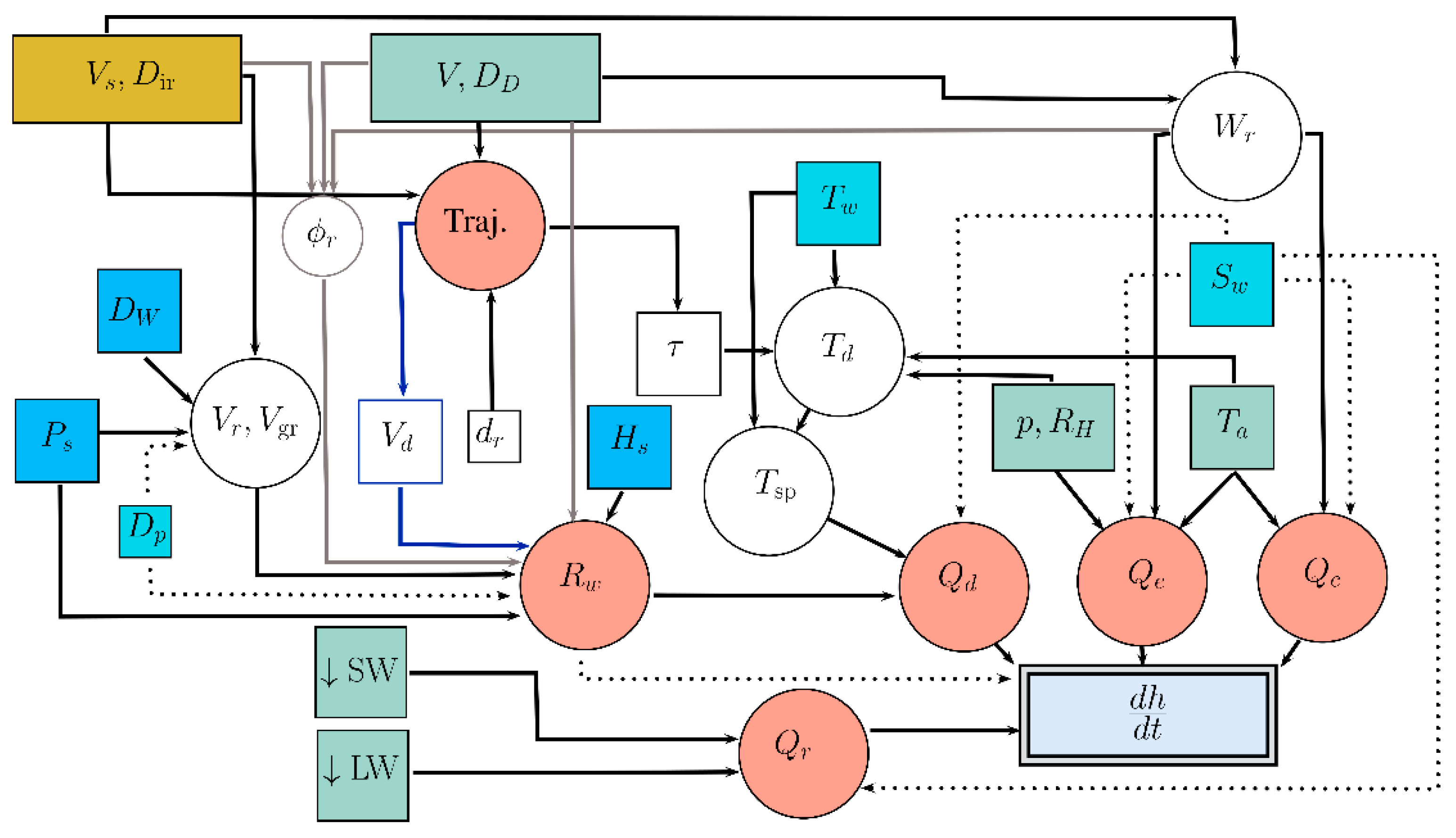
2.1. MINCOG Model Description, Study Assumption, and Data

The MINCOG model [1] is developed based on the modelling of wave-ship interaction and uses the Norwegian Coast Guard ship class named "KV Nordkapp" as a reference ship type for ship-icing calculations. The sea-spray flux $R_w$, in the MINCOG model, is calculated based on spray data adapted from Borisenkov et al. [29] and Horjen et al. [30] and adjusted for the larger size of the “KV Nordkapp” ships compared to the ships where the spray data were collected. The spray flux is also calculated at the position in which icing was recorded on the KV Nordkapp ships by using a trajectory model for droplet speed and droplet flight time, which depends on the ship geometry of KV Nordkapp. In addition, a heat balance is assumed at this fixed position in the front of the ship, and the icing rate $dh/dt$ is derived by considering the most important heat fluxes $Q$, acting on the saline water on this position of the ship. As salt is expelled during the freezing process, the freezing temperature is lower than the freezing temperature of the incoming seawater. Figure 1 illustrates the MINCOG model-system flow chart adopted from Samuelsen et al. [1]. The model uses 15 input variables from the atmosphere (green), the ocean waves (blue), the ocean (turquoise), and the ship (yellow). However, in this study only the parameters that are directly available from NORA10 are applied as inputs to the model, i.e., wind speed $V$, air temperature $T_a$, relative humidity $R_H$, mean-sea level pressure $p$, significant wave height $H_s$, and significant wave period $P_s$.

For the other parameters, the mean value in Table 2 in Samuelsen et al. [1] is applied as input, namely a constant vessel speed $V_s$ of 4 m s⁻¹, sea surface or water temperature $T_w$ of 2.5 °C, and incoming seawater salinity $S_w$ of 35 ppt. According to the sensitivity tests performed by Samuelsen [16], it was both calculated and observed that icing rates are not very sensitive to $V_s$, $T_w$, or $S_w$ in the observed ranges of these parameters in the sea areas of interest. Furthermore, deep-water approximation is applied, so the bathymetry depth $D_P$ is not needed for wave-phase speed calculation.

Moreover, incoming shortwave radiation $\downarrow SW$ is neglected, and incoming longwave radiation is parametrized by assuming that the atmosphere is radiating as a black body with a temperature equal to the 2-metre air temperature, i.e., $\downarrow LW=\sigma {\left(T_a+273.15\right)}^4$, where $\sigma$ is the Stefan-Boltzmann constant, $5.6710\times {10}^{-8}$ Wm⁻²K⁻⁴. Furthermore, it is assumed that the winds and waves are coming from the same direction, i.e., $DD=DW$, and a constant angle is applied for the direction between the ship and wind equal to the median value of the icing events used in Samuelsen et al. [1], i.e., $\beta =\left|D_{ir}-D_D\right|=150 °$. The trajectory model is skipped for simplicity and the water droplet velocity $V_d$ is calculated from the relative velocity between the wind and the ship in the horizontal direction, and an assumed terminal velocity of uniform droplets with a constant spherical size with a diameter of 2 mm. Furthermore, only the spray-flux expression with spray data adapted from Reference [30] is applied. For further details on the modelling steps and algorithms employed in MINCOG, the reader is referred to the work done by Samuelsen et al. [1] and Samuelsen [3].

Meteorological and atmospheric parameters contributing to the spray-ice generation and its accretion rate are time-dependent and also vary over the Arctic. This, consequently, leads to a spatial-temporal variation of icing event occurrence and accretion rate, which should be studied over the region, where offshore installations are located, or over sea voyages, wherein logistics support and shipping operations are performed. To this aim, the 3-hourly reanalysis hindcast (NORA10) database is used to extract the values of the six variable input parameters of the MINCOG model, i.e., wind speed $V$, air temperature $T_a$, relative humidity $R_H$, mean-sea level pressure $p$, significant wave height $H_s$, and significant wave period $P_s$. NORA10 is a downscaling of the global reanalysis ERA-40 [31] from 1958 to 2002. The downscaling is performed over the Northern Atlantic with the HIgh Resolution Limited Area Model (HIRLAM) version 6.4.2 [32] set up on a rotated grid with approximately 0.1 degree resolution (approximately 10 km grid spacing) [33]. The WAve Model (WAM) [34] is forced from HIRLAM on the same grid. After the year 2002, the operational analyses from the European Centre for Medium-Range Weather Forecasts Integrated Forecasting System (ECMWF IFS) are applied initially and at the boundary of HIRLAM. In this study, the period, for which 3-hourly NORA10 data are extracted, is from 1 January 1980 to 31 December 2012, which constitutes more than 96,000 sets of input data for estimation of icing rate using the MINCOG model for such a period.

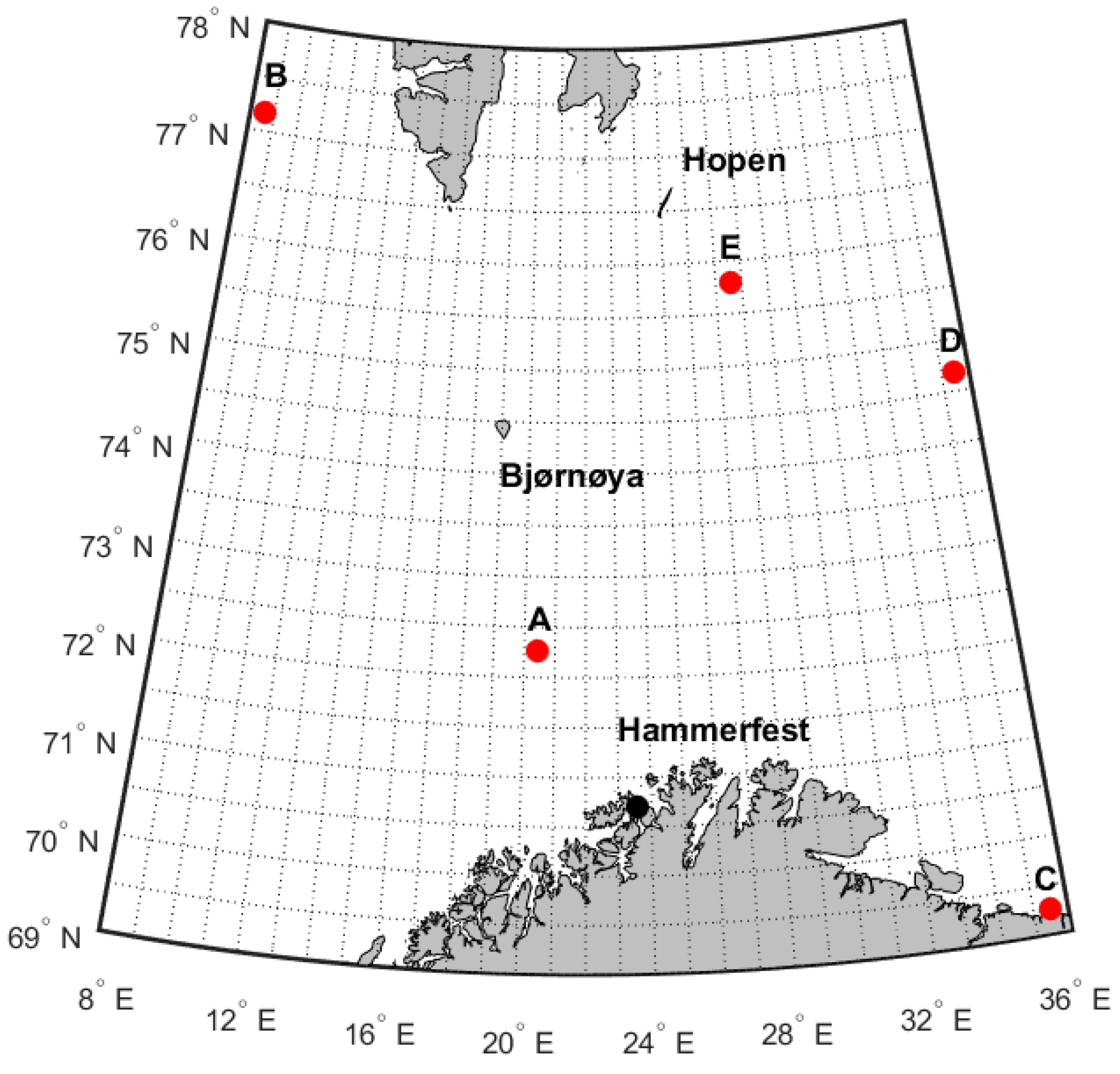
2.2. Scope of the Study and Grid Preparation

Figure 2 illustrates the scope of the study that mainly covers the Arctic Norwegian sea areas. The area is bounded to the latitudes 69° N to 78° N divided into 18 meridians each of which is 0.5 degrees; and, to the longitudes 8° E to 36° E divided into 28 parallels, each of which is 1 degree. This divides the whole area into 441 grid cells excluding the grids covering the land. Five different offshore locations, denoted by A (72.49° N, 20.37° E), B (77.18° N, 8.61° E), C (69.26° N, 35.50° E), D (74.07° N, 35.81° E), and E (75.80° N, 27.60° E), as illustrated in Figure 2, are selected based on their potential interest from either industrial or meteorological perspectives for a more detailed analysis of temporal variability of meteorological and oceanographic parameters and, thus, icing events and icing rates.

Location A (72.49° N, 20.37° E) corresponds to 7220/8-1 discovery wellbore in the Skrugard structure of Johan Castberg O&G field in the southwest of the Barents Sea, discovered in 2011. The planned development concept includes a production, storage, and offloading vessel [35]. As illustrated in Figure 3, the water system in location A is a mixture of coastal waters and warm Atlantic waters flowing towards the northeast. Activities related to drilling, field development, and production, in addition to the introduction of some passive safety barriers such as deployment of vessels and facilities for oil spill containment and removal, as well as search and rescue vessels, highlight the necessity of acquiring detailed information on the possibility of icing events and icing rates throughout the year at this location. Location B (77.18° N, 8.61° E) is west of Spitsbergen island in the Svalbard archipelago, where the main water stream is the continuation of warm Atlantic waters flowing towards the northwest of Svalbard (see Figure 3). Location C (69.26° N, 35.50° E) is at the Russian coast in the Barents Sea, north of Murmansk, which is important for offshore vessel operations and supporting activities that are involved with the development and production of Russian gas fields located further north in the east of the Norwegian-Russian sea border, like Shtokman, Ledovoye, and Ludlovskoye [36]. The main water system at this location is the coastal water flowing towards the east. Location D (74.07° N, 35.81° E) is where the discovery wellbore 7435/12-1 was drilled in 2017 in the Norwegian part of the Barents Sea [37]. It is located approximately 500 km east of Bjørnøya (see Figure 3). This grid cell is in the northeast of the area, which is currently open for petroleum activity in the Norwegian Barents Sea (delineated below the latitude 74.5° N). Location E (75.80° N, 27.60° E) is in the southwest of Hopen Island, near the sea ice edge, where cold Arctic waters meet warm Atlantic waters (see Figure 3). Although this area is not open for petroleum activities, it had been licensed for conducting seismic surveys [37].

3. Results and Discussion

3.1. Icing Events and Their Rates in Some Regions of Interest

According to Samuelsen [16], only three atmospheric or oceanographic parameters contribute to the icing rate significantly, namely wind speed, air temperature, and significant wave height. Figure 4 shows the daily variation of wind speed in m s⁻¹, significant wave height in m, and air temperature in °C, in locations A to E (see Figure 2). Each plot shows the 2.5th percentile (blue), the median (black), and the 97.5th percentile (red) of the corresponding variable. Such values are obtained by collecting the data corresponding to each day over the course of 33 years from 01.01.1980 to 31.12.2012, and then computing the required statistics for each day. The values of -1 referring to significant wave heights in locations D and E represent the cases where the sea surface was covered by ice and thus no wave heights were recorded. It is trivial that, on such occasions, no spray icing occurs either. Compared to the other locations, location A has relatively higher air temperature throughout the year with a median approximately above zero, which is due to the flow of relatively warmer Atlantic waters (see Figure 2). The air temperature difference between summer and winter in location A is also smaller than that of the other locations. Locations B, D, and E, which are near the ice edge and located further away from the Atlantic water current, have lower temperatures in general, specifically during winter with a relatively larger difference between summer and winter air temperatures. The temporal temperature profile of location C shows relatively warmer summer seasons and colder winter seasons than those of A, a clear signature of point C being closer to the land areas compared to the open ocean point A. Hence, C is more affected by the temperature onshore during both summer and winter. Location C has also relatively weaker wind speeds and lower wave heights than A, particularly in winter. One interpretation of the weaker wind speed in C relative to A might be that the cyclones could be a more attenuated when they pass the land areas of Northern Scandinavia, and therefore they would produce weaker winds in C. However, it might also be due to the fact that point C is so close to the land points in the model with higher roughness compared to point A, which is only surrounded by ocean points. The lower waves in C compared to A might be a result of the weaker winds in C but may also stem from the fact that there is clear fetch limitation even in strong wind conditions when the wind is blowing from the land in C, i.e., the waves are not building up so close to the shore. As stated earlier, sea surfaces in locations D and E are sometimes frozen in winter, thus the lower 2.5th percentile of wave height in those regions is represented by −1. It is also interesting to note that the air-temperature median in A is mostly above zero degrees throughout the year, while in the other four locations the median is below zero degrees from October/November to April/May.

The first row of Figure 5 illustrates the icing-rate distribution in cm h⁻¹ for each month in locations A to E. Icing rates are obtained by collecting the icing rate values corresponding to each day of the year over the course of 33 years from 1 January 1980 to 31 December 2012. In other words, for each specific day of the year there are 33 icing rate values, for which the corresponding 2.5th percentile (blue), the median (black), and the 97.5th percentile (red) are estimated. In addition, it is also useful to have an estimate of the probability of the occurrence of an icing event on each day throughout the year, or an average in each month. To this aim, for each calendar year (i.e., 1980 to 2012) the number of icing events during each month is divided by the total number of time intervals (each day includes eight equal time intervals) in order to compute the 3-hourly frequency of icing events in each month of each year. For example, an icing frequency of 37.5% for January means that 93 icing events occurred during that month, which are divided into 248 (31 times 8) 3-hour time intervals. This will result in 33 different values of a 3-hourly icing event frequency corresponding to each month. Such values are further used to estimate the 2.5th percentile, the median, and the 97.5th percentile for that month, which are illustrated in the boxplots shown in the second row of Figure 5.

Higher air temperatures throughout the year lead to a smaller ice accretion rate in location A compared to other locations, while, in location C, such a relatively lower ice accretion rate is mainly due to the lower wave height and, thus, smaller water flux compared to the other locations. Locations B, D, and E experience higher accretion rates compared to the other locations. Since the wave height and wind speed climatology in B, D, and E are quite similar to those of A (Figure 4), such higher accretion rates are then due to lower air temperatures in those regions. In winter and spring (December to May), locations D and E experience a large variation of icing frequency (the second row of Figure 5), which could be related to the fact that the sea surface is frozen throughout the month in some years, providing no icing, while in some other years there are only certain days with sea ice during these months. Location A, in the southwestern Barents Sea, has a relatively lower icing frequency compared to the other locations (the second row of Figure 5), which is mainly associated with higher air temperatures in A. On the other hand, the frequency of icing events in location C is considerably higher than that of A.

Moreover, as illustrated in the second row of Figure 5, in all these locations no icing events are recorded in August. In locations A and C, this icing-free period includes June, July, and September; and, in location B, the only ice-free months are July and August. Such trends are also confirmed by notably above-zero air temperatures in those months as shown in Figure 4. It is also apparent from the second row of Figure 5 that, in location A, the minimum icing frequency for all the months is zero. In other words, there has been at least a year over the whole period of 33 years that no icing event has happened in either of the months in location A. Similarly, the first few months of the year in locations D and E have also a minimum icing frequency equal to zero, which is related to either occasional positive air temperatures or frozen sea surface. On the other hand, in locations B and C, there are no icing-free winter months, i.e., for each of these winter months, there have always been some icing events over the whole period of 33 years.

While the second row of Figure 5 reports the 2.5th, 50th, and 97.5th percentiles of icing frequency regardless of its severity level, Figure 6 distinguishes the icing frequency of each location corresponding to three different severity levels, namely light (L) (the first row), moderate (M) (the second row), and severe (S) (the third row). The data for constructing the boxplots in Figure 6 are restructured in the same way as the data applied for Figure 5. Samuelsen [16] divides icing events into light, moderate, and severe classes according to the frequency distribution of observed icing rates combined with reported severity of severe icing events from the Norwegian Coast Guard. Moderate class represents the icing rates above the 50th percentile of observed icing rates in Samuelsen [16], while severe icing class includes those events with rates above the 90th percentile, both assuming that the icing rates are following a log-normal distribution [16]. The applied thresholds represent the expected ice accumulation on the fixed position of the KV Nordkapp ships and are given by Equation (1):

$$\mathrm{Icing}\mathrm{Class}=\{\begin{array}{c}\mathrm{Light} 0.05\le \frac{dh}{dt}<0.5\\ \mathrm{Moderate} 0.5\le \frac{dh}{dt}<1.34\\ \mathrm{Severe} 1.34\le \frac{dh}{dt}\end{array},$$

(1)

Note that, as presented by Equation (1), icing rates smaller than 0.05 cm h⁻¹ are assumed zero by following the categorization procedure of Samuelsen [16] in order to avoid unrealistically small rates in the light icing class.

As shown in Figure 6, while most of the icing events occurred in locations A and C are categorized as light, the frequency of moderate icing events in locations B, D, and E are considerable, particularly during winter months. In addition, as shown in the last row of Figure 6, no severe icing is recorded for locations A and C, while some winter months in locations B, D, and E have experienced severe icing events, although with lower frequencies compared to moderate and light icing events in such locations.

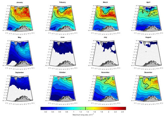
3.2. Spatial-Temporal Variation of Icing Rate and Frequency over the Arctic Norwegian Sea Areas

Figure 7 illustrates the maximum icing rate in cm h⁻¹ for the sea areas between Northern Norway and Svalbard during each month over a period of 33 years, starting from 1 January 1980 using more than 96,000 sets of meteorological and atmospheric data. The reasoning behind reporting the maximum icing rate is related to the design and operational concerns. The proposed engineering solutions for design facilities and their operations in the Arctic offshore should be able to withstand at least such icing events. This information can be used for the implementation of anti- and de-icing techniques. Although these icing rates correspond to a period of 33 years in the past, one can also account for temporal variation of maximum icing rates and their frequency over this period in order to obtain some predictions of extreme values (e.g., 100-year or 10,000-year return period) for maximum icing rates. The thresholds for moderate/severe icing rates are specified by solid black lines in the plots and legend.

Figure 8 shows the 3-hourly frequency of icing events, including all icing classes, i.e., light, moderate, and severe (Equation (1)) in each month. Frequencies are obtained by dividing the total number of icing events occurring in each month during the period 1980 to 2012 by the total number of time intervals. For instance, for January, the total number of time intervals is $8\times 31\times 33=8184$, and the number of icing events is the number of times that estimated icing rate is greater than or equal to 0.05 cm h⁻¹. This ratio is calculated and reported as the 3-hourly frequency of icing events. The solid black contour line in the plots and solid black line in the color bar legend show the 50% frequency.

Alternatively, for each grid cell, one can obtain an icing rate distribution for each month or day. One might be also interested in the distribution or percentiles of the distribution of icing frequency for a specific location for each day or month. An example of such results is shown in Figure 5 and Figure 6 for five selected locations in the Norwegian Arctic sea areas (see Figure 2).

Sometimes decision-makers are interested in moderate/severe icing events in order to adapt specific anti-icing and de-icing measures that would not be necessary for light icing events. In Figure 9, the 3-hourly frequency of the combined class moderate and severe icing in each month is visualized. The solid black contour lines specify the 10% and 20% frequencies. The approach followed for estimating such frequencies is the same as the one used for constructing Figure 8. However, this case excludes the icing events with a rate smaller than 0.5 cm h⁻¹ (i.e., excluding light icing events), and thus just represents the 3-hourly frequency of moderate and severe icing events.

Figure 7 and Figure 8 indicate that icing has occurred in all months in the northernmost part of the region, while Figure 9 visualizes that moderate or severe icing has never occurred in the summer months of June to August. The most severe events have occurred in January to March north of 74° N (Figure 7), and mainly east of Spitsbergen. On the other hand, the highest icing frequency is west of Spitsbergen and near the coast of Russia, corroborating the results from points B and C in the second row of Figure 5. It is clearly noticeable in Figure 8 that the the icing frequency is lower in the northeastern part of the region, where sea ice normally occurs from November to April compared to the region further south and west with the highest icing frequencies. This highlights the complexity of the spray-icing problem, which is needed when considering both the spray available for freezing and the heat fluxes capable of freezing the brine water.

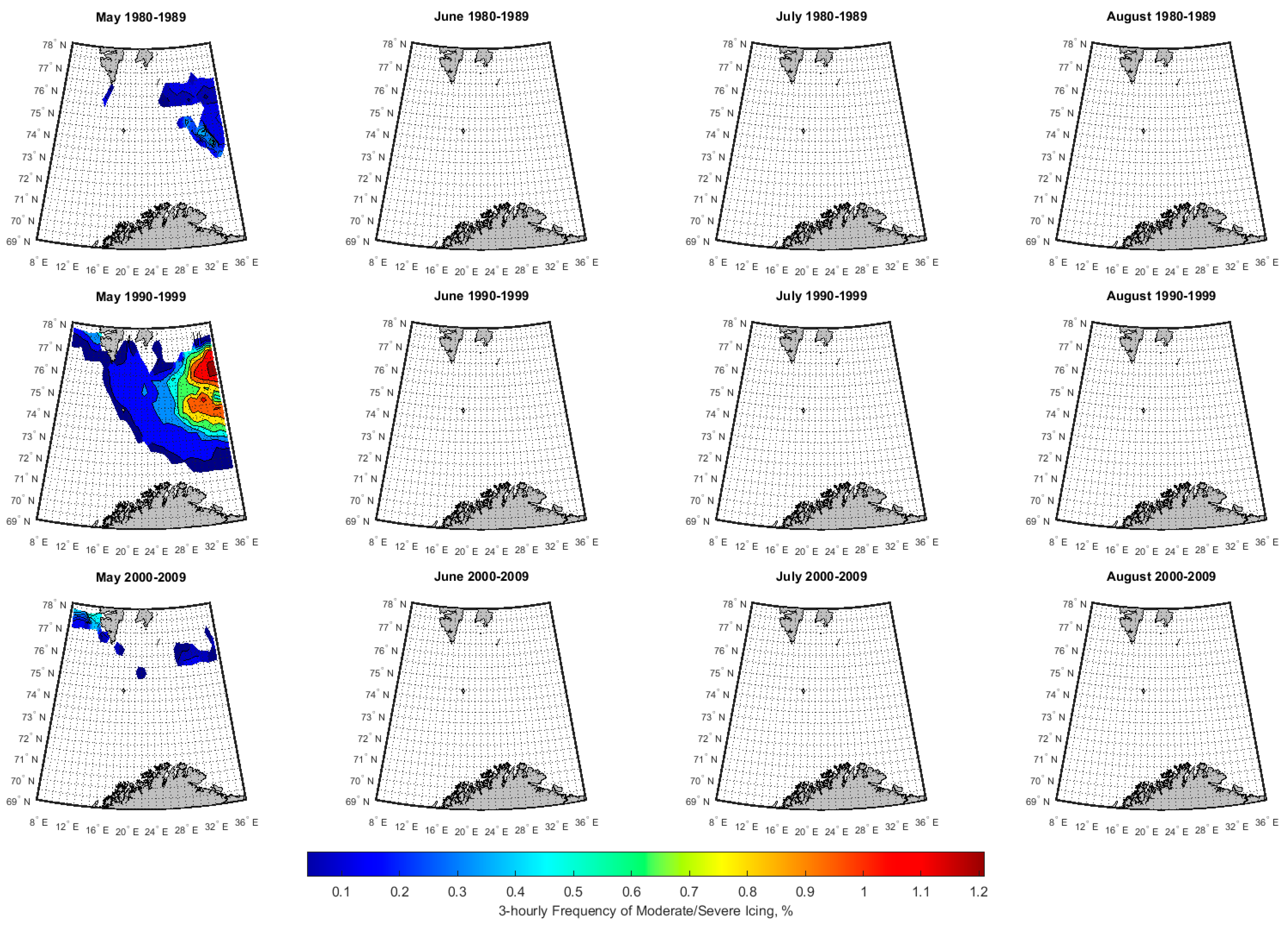
3.3. Historical Trend of Icing Rates and Frequencies over the Arctic Norwegian Sea Areas

Although the Arctic has always experienced cooling and warming cycles, the current meltdown, which is dramatic and directly correlated with industrial emissions of greenhouse gases, defies any historical comparison [39]. In general, the effects of global warming in the Arctic are far more dramatic than elsewhere, which is a fact that has led to the retreat of sea ice over recent decades. Since 1995, at least 41% of multiyear ice has vanished from the Arctic Ocean [40]. This is also evident in the Norwegian Meteorological Institute’s data confirming that the area of the Arctic Ocean, with at least 15% sea ice concentration, has decreased considerably over the last three decades (1979–2010), with a relatively sharper decreasing trend during summer and autumn. From 1981 to 2010, the ice extent in summer has diminished by 30%, while it has reduced by 10% during winter, with the lowest record occurring at end of summer 2012 since 1979. Similar to other Arctic seas, the Barents Sea has also experienced a reduction in ice extent. According to the data provided by the Norwegian Meteorological Institute on the sea-ice extent with at least 15% ice concentration from 1980 to 2015 in April, there is a clear decreasing trend from about 880 km² in 1980 to about 607 km² in 2017 (about 30%) with the lowest record of about 458 km² in 2016.

Such a decreasing trend of sea-ice area can also be interpreted in terms of the retreat of sea-ice edge. Figure 10A,B show the frequency of sea ice extent with at least 40% ice concentration over the period October 1980 to May 1981 and October 2011 to May 2012, respectively, over the central and western Barents Sea. As shown in these figures, the position of the ice edge in the Barents Sea with at least 40% ice concentration has changed considerably during the period 1980 to 2012. For instance, while in the winter of 1980 the areas northeast of Svalbard had always been covered by sea ice with a concentration of at least 40%, the frequency of the sea surface being covered with such an ice concentration varies between 40% to 100% in the winter of 2011. Central parts of the Barents Sea, areas west of Svalbard and north of Bjørnøya, show a considerable retreat of ice edge.

The loss of sea ice significantly raises the absorbed surface solar radiation and the heat loss from the ocean surface through turbulent heat fluxes between the ocean and atmosphere and outgoing longwave radiation from the ocean surface. A combination of these factors, together with the lateral heat transport into the Barents Sea, determine the changes in sea surface temperature [41]. In general, both observations and simulations suggest a clear increasing trend in surface temperature of the Barents Sea over recent decades, although there are some inter-annual and decadal variations [41,42]. In addition to the sea surface temperature, the Barents Sea air temperature has also increased during recent decades. In addition to its effects on sea surface temperature and air temperature, the loss of sea ice and the retreat of the sea ice edge contribute to changes in significant wave heights, particularly in areas close to the ice edge, where sea ice normally occurred during certain months of the year in the past.

Such complex long-term changes in meteorological and oceanographic parameters of the Barents Sea affect the occurrence of spray icing and icing rate in the long term. Thus, regarding the planning for design and operations of industrial facilities and activities in the Norwegian Arctic sea areas in general and the Barents Sea in particular, one should definitely account for annual and decadal changes in spray icing frequency and rates. In order to illustrate this issue, an arbitrary position in the east of Hopen Island is selected, as shown in Figure 10, denoted by X (77.2° N, 32.5° E). Figure 11 shows the annual variation of the median of significant wave height and mean air temperature in this location for months January to May and October to December from 1980 to 2012. The values of −1 referring to significant wave heights represent the cases where the sea surface was covered by ice and thus no wave heights were recorded. In the period October 1980 to May 1981, location X has experienced a sea ice concentration of at least 40% with a frequency of approximately 60%–70%. However, such a frequency reduces to zero percent in the period October 2011 to May 2012. As depicted in Figure 11, the retreat of sea ice then becomes associated with the increase in significant wave height, especially in January, November, and December in recent years. In addition, for the same period, Figure 12 shows yearly variations in estimated 3-hourly icing frequency and the 97.5th percentile of icing rates in this location. The increase in icing frequencies, particularly in November, December, and to some extent, in January, is the most noticeable signature in these figures, a clear result of decreasing sea ice and retreat of sea ice edge. Since the temperature is still below freezing, in combination with high enough waves and strong enough winds, icing will still occur, although the air temperature experiences a rising trend.

As indicated by Figure 11 and Figure 12, it is of particular importance for the industries to have clearer information and knowledge about long-term changes of spray icing occurrence frequency and rate. To this aim, Figure 13, Figure 14 and Figure 15 show the 3-hourly frequency of all icing classes in each month over the whole region. The first, second, and third row of the figures compare icing frequencies during the periods 1980–1989, 1990–1999, and 2000–2009, respectively. Similarly, in Figure 16, Figure 17 and Figure 18, the 3-hourly frequencies of severe and moderate icing events in each month over the whole region are presented. The first, second, and third row of these figures compare severe and moderate icing frequencies during the periods 1980–1989, 1990–1999, and 2000–2009, respectively.

Investigation of the plots in Figure 13, Figure 14, Figure 15, Figure 16, Figure 17 and Figure 18 reveals several interesting results. Firstly, the southwestern corner seems to have a reduction or little trend in icing frequency when comparing the 1980s, 1990s, and 2000s for each month. For the northwestern corner, there also seems to be a decreasing trend in some of the months, particularly November, December, and January. However, considering all icing classes, in February, and particularly March, the icing frequency in the 2000s is almost equal or even higher than in the 1980s. The month of March in the 2000s actually seems to have the highest icing frequency in this area among all months during these three decades. This may be related to more cold air outbreaks from the ice, i.e., events with strong winds, high waves, and low temperatures in combination, in this month in the 2000s compared to the other months. When investigating the frequency of the combined moderate and severe icing for the month of March, the same signature is apparent, i.e., the 2000s have the highest icing frequency and the 1990s have the lowest (Figure 16). Additionally in April, there is no apparent decreasing trend in icing frequencies in the northwestern corner among the three decades; and, regarding the frequency of moderate and severe events, the highest value is associated with the 2000s. However, a clear decreasing trend is apparent in moderate/severe icing frequency in this region in February from the 1980s to the 2000s.

In the northeastern corner, south of the ice edge, a similar pattern in March and April is apparent. In addition, it is noticeable that, in November and December, there is a clear increasing trend in icing frequencies in the northeastern corner, where the sea surface was usually covered by sea ice during the 1980s and the 1990s, and not in the 2000s. In fact, this illustrates that the effect of global warming on icing frequency is more complex and sophisticated than one may initially anticipate, namely that it is not necessarily a decreasing trend of icing frequency in all months, even though the Arctic is getting warmer. Thus, the stream pattern affecting the temperature, wind, and wave conditions in certain areas plays a crucial role. There has, for instance, been pinpointed that one effect of global warming and the Arctic amplification might be the wavier jet streams [43], with more consistent northerlies or southerlies during longer periods of a month in the future. Hence, months with more consistent northerlies combined with sub-freezing conditions may result in higher frequencies of icing also in the future. However, at some point the atmosphere may become too warm in the winter season for icing to occur at all.

A further interpretation of the results in Figure 13, Figure 14 and Figure 15 might be that the seasons in these areas have been extended and shifted. In other words, the extension of the autumn season into November and December in some years, due to longer periods of warm-air advection, may result in an extension of the most intense winter season into March due to processes and teleconnections in the atmosphere that are not fully understood. Furthermore, some icing events have occurred during summer in later decades, which are not apparent in the 1980s. However, the number of events is very small, suggesting that they might also be a result of random decadal variation.

4. Application in Risk-Based Decision-Making

One of the applications of the results of this study is providing decision-makers with inputs regarding spray icing frequencies and rates that will be used in risk analyses and making informed decisions on different aspects of Arctic offshore industrial activities, including scheduling and routing of offshore supply vessels, sailing of fishing vessels, conducting offshore search and rescue operations, and offshore oil spill clean-up operations. For the short-term and real-time decision-making tasks, weather data are usually available with an acceptable level of uncertainty. Such data can be used in the MINCOG model for estimation of icing rates in the period of interest in the short term and/or real time.

However, the design and operation of Arctic offshore facilities and industrial activities require knowledge on long-term associated risks, in general, and spray icing risk in particular. As spray icing poses risks to industrial activities, some risk reducing measures should be implemented to reduce the risks below an acceptable level. This can be achieved in different ways such as implementing design modifications (e.g., vessel winterization), or developing some internal regulations and practices (e.g., warnings for icing) for operators and decision makers. However, the main purpose of this study is to provide decision makers with inputs during operation phase and also during planning an activity (e.g., routing and scheduling a fleet of offshore supply vessel). In this regard, a statistical representation of icing rates and frequency can play a very useful role for risk-informed decisions. Thus, the statistics of icing rates and frequency, which are presented in this study (i.e., the 95% confidence bound, median, and mean) can be used as inputs for comparing the risks against some acceptable levels, and thus for identifying the most dangerous situations, to which a combination of different technical and organizational risk reducing measures should be in place to avoid catastrophes.

There are, in principle, two approaches for the estimation of icing rates and prediction of icing events. In the first approach, the key variables of the MINCOG model, including wind speed, air temperature, relative humidity, mean-sea level pressure, significant wave height, and significant wave period, are simulated at junctures of interest in future. Such a simulation is conducted from distribution functions obtained from available meteorological and atmospheric data, which in this study are 3-hourly hind-cast data from 1 January 1980 to 31 December 2012. Once input parameters are simulated, they can be plugged in the MINCOG model for icing rate estimation for corresponding junctures. After repeating such a simulation process for a sufficiently large number of times, the statistics of the associated risks, fuel consumption for winterization purposes, and possible delays due to heavy icing events can be obtained.

Alternatively, estimated values of icing rates for the period 1 January 1980 to 31 December 2012 can be used to simulate icing rates at future junctures. To this aim, a non-sequential Monte Carlo simulation [44] can be used to randomly simulate icing rates for any region of interest at any juncture. In this regard, a two-step sampling approach can be used [45]. In this first step, the occurrence or non-occurrence of an icing event is simulated using 3-hourly icing frequencies. If an icing event occurs, the icing rate will then be simulated using corresponding icing rate distribution functions. An example of this approach is illustrated by Naseri and Samuelsen [45], where the icing rate and equivalent amount of heat loss due to implementation of anti-icing measures are estimated for a sea voyage in the Barents Sea for a given period. A similar approach is also used by Teigen et al. [24] where historical icing rates and a corresponding mass of accreted ice on floating O&G installations are fitted to a parametric distribution function in order to estimate the required extreme values such as 100-year and 10,000-year return periods.

Moreover, some of the O&G projects and activities are usually planned to last for the following couple of decades (e.g., an oil spill clean-up plan for a production platform that is designed to produce for the next 20 years). Due to climate change, sea-ice cover trend and sea-ice edge position are expected to change in future as suggested by their historical trend over recent decades. This issue, which is discussed in detail in this study, therefore calls for employing more advanced sampling techniques such as sequential Monte Carlo simulation [44], for simulation of icing events and icing rates at future junctures in order to account for long-term spray icing risks.

5. Conclusions and Recommendations

This paper adapts a newly developed ship-icing model known as MINCOG. By using 3-hourly NORA10 data, icing rates are estimated for some Arctic sea areas for the period 1 January 1980 to 31 December 2012, which were further used to study the climatology of spray icing in such Arctic offshore regions. Spray icing maps showing the maximum icing rates and 3-hourly frequencies are developed for the areas of interest corresponding to three different icing categories, namely severe, moderate, and light. In addition, spray icing and its relation to wind speed, significant wave height, and air temperature are discussed in detail for five different locations selected in the Norwegian Arctic sea areas.

The presence of sea ice, and its following limitation of spray water, is of great importance; a fact that is strongly highlighted through the figures in this study. The presented changes and trends in icing frequencies throughout three decades is also of great interest and has not been highlighted earlier. Although many studies have been focused on the possibilities for increased marine activity and oil and gas operations in Arctic sea waters when the sea ice is retreating [46,47], this study highlights that spray icing is not necessarily retreating in the same manner. In fact, an increase in icing frequency is apparent in March and April in the latest decade that is considered, compared to earlier decades.

The results of this study indicate the spatial-temporal variations of icing rates, severity, and frequency over the selected Arctic sea areas. The results of this study can be used for Arctic offshore risk analyses and making risk-informed decisions. Further research should be revolved around developing approaches for simulation of meteorological and atmospheric parameters, while taking into account their long-term trends in order to develop a framework for long-term simulation of icing events in a specific area.

References

1. Samuelsen, E.M.; Edvardsen, K.; Graversen, R.G. Modelled and observed sea-spray icing in Arctic-Norwegian waters. Cold Reg. Sci. Technol. 2017, 134, 54–81. [Google Scholar] [CrossRef]
2. Dehghani-Sanij, A.R.; Dehghani, S.R.; Naterer, G.F.; Muzychka, Y.S. Sea spray icing phenomena on marine vessels and offshore structures: Review and formulation. Ocean Eng. 2017, 132, 25–39. [Google Scholar] [CrossRef]
3. Samuelsen, E.M. Prediction of ship icing in Arctic waters—Observations and modelling for application in operational weather forecasting. Ph.D. Thesis, UiT The Arctic University of Norway, Tromsø, Norway, 2017. [Google Scholar]
4. Chatterton, M.; Cook, J.C. The Effects of Icing on Commercial Fishing Vessels; Worcester Polytechnic Institute: Worcester, UK, 2008. [Google Scholar]
5. ISO. ISO 12494: Atmospheric Icing of Structures; ISO: Geneva, Switzerland, 2017. [Google Scholar]
6. Ryerson, C.C. Assessment of Superstructure Ice Protection as Applied to Offshore Oil Operations: Safety Problems, Hazards, Needs, and Potential Transfer Technologies; US Army Engineer Research and Development Center: Hanover, NH, USA, 2008. [Google Scholar]
7. Jones, K.F.; Andreas, E.L. Sea Spray Icing of Drilling and Production Platforms; US Army Engineer Research and Development Centre: Hanover, NH, USA, 2009. [Google Scholar]
8. Barabadi, A.; Garmabaki, A.H.S.; Zaki, R. Designing for performability: An icing risk index for Arctic offshore. Cold Reg. Sci. Technol. 2016, 124, 77–86. [Google Scholar] [CrossRef]
9. Kulyakhtin, A.; Tsarau, A. A time-dependent model of marine icing with application of computational fluid dynamics. Cold Reg. Sci. Technol. 2014, 104–105, 33–44. [Google Scholar] [CrossRef]
10. Naseri, M.; Barabady, J. On RAM performance of production facilities operating under the Barents Sea harsh environmental conditions. Int. J. Syst. Assur. Eng. Manag. 2016, 7, 273–298. [Google Scholar] [CrossRef]
11. Ryerson, C.C. Ice protection of offshore platforms. Cold Reg. Sci. Technol. 2011, 65, 97–110. [Google Scholar] [CrossRef]
12. Rashid, T.; Khawaja, H.A.; Edvardsen, K. Review of marine icing and anti-/de-icing systems. J. Mar. Eng. Technol. 2016, 15, 79–87. [Google Scholar] [CrossRef]
13. DNV. DNV-OS-A201: Winterization for Cold Climate Operations; DNV: Høvik, Norway, 2013. [Google Scholar]
14. Moore, G.W.K. A climatology of vessel icing for the subpolar North Atlantic Ocean. Int. J. Climatol. 2013, 33, 2495–2507. [Google Scholar] [CrossRef]
15. Lozowski, E.P.; Szilder, K.; Makkonen, L. Computer simulation of marine ice accretion. Philos. Trans. R. Soc. Lond. A Math. Phys. Eng. Sci. 2000, 358. [Google Scholar] [CrossRef]
16. Samuelsen, E.M. Ship-icing prediction methods applied in operational weather forecasting. Q. J. R. Meteorol. Soc. 2018, 144, 13–33. [Google Scholar] [CrossRef]
17. Mertins, H. Icing on fishing vessels due to spray. Mar. Obs. 1968, 38, 128–130. [Google Scholar]
18. Dehghani-Sanij, A.R.; Dehghani, S.R.; Naterer, G.F.; Muzychka, Y.S. Marine icing phenomena on vessels and offshore structures: Prediction and analysis. Ocean Eng. 2017, 143, 1–23. [Google Scholar] [CrossRef]
19. Hansen, E.S.; Eik, K.J.; Teigen, S.H. Statistical Methods for Applying Icing Estimates in Offshore Design. In Proceedings of the 23rd International Conference on Port and Ocean Engineering under Arctic Conditions (POACT15), Trondheim, Norway, 14–18 June 2015. [Google Scholar]
20. Horjen, I. Numerical modeling of two-dimensional sea spray icing on vessel-mounted cylinders. Cold Reg. Sci. Technol. 2013, 93, 20–35. [Google Scholar] [CrossRef]
21. Horjen, I. Numerical Modelling of Time-dependent Marine Icing, Anti-icing and De-icing; Norges Tekniske Høgskole (NTH): Trondheim, Norway, 1960. [Google Scholar]
22. Forest, T.W.; Lozowski, E.P.; Gagnon, R.E. Estimating Marine Icing on Offshore Structures Using RIGICE04. In Proceedings of the 11th International Workshop on Atmospheric Icing of Structures, Montreal, QC, Canada, 12–16 June 2006. [Google Scholar]
23. Overland, J.E. Prediction of vessel icing for near-freezing sea temperatures. Weather Forecast. 1990, 5, 62–77. [Google Scholar] [CrossRef]
24. Teigen, S.H.; Hansen, E.S.; Roth, J.C. Marine Icing Severity in the Barents Sea. In Proceedings of the 23rd International Conference on Port and Ocean Engineering under Arctic Conditions (POAC15), Trondheim, Norway, 14–18 June 2015. [Google Scholar]
25. Løset, S.; Vefsnmo, S.; Karas, J.; Kelly, M. Environmental Conditions in the Barents Sea in Regard to Icing. In Proceedings of the International Conference on Technology for Polar Areas (Polartech), Trondheim, Norway, 15–17 June 1988; Volume 2, pp. 393–407. [Google Scholar]
26. Samuelsen, E.M.; Løset, S.; Edvardsen, K. Marine icing observed on KV Nordkapp during a cold air outbreak with a developing polar low in the Barents Sea. In Proceedings of the 23rd International Conference on Port and Ocean Engineering Under Arctic Conditions (POAC15), Trondheim, Norway, 14–18 June 2015. [Google Scholar]
27. Feit, D.M. Forecasting of superstructure icing for Alaskan waters. Natl. Weather Dig. Mar. 1987, 12, 5–10. [Google Scholar]
28. Reistad, M.; Breivik, Ø.; Haakenstad, H.; Aarnes, O.J.; Furevik, B.R.; Bidlot, J.R. A high-resolution hindcast of wind and waves for the North Sea, the Norwegian Sea, and the Barents Sea. J. Geophys. Res. Ocean. 2011, 116. [Google Scholar] [CrossRef]
29. Borisenkov, Y.P.; Zablockiy, G.A.; Makshtas, A.P.; Migulin, A.I.; Panov, V.V. On the approximation of the spray-cloud dimensions. In Trudy Arkticeskogo; Romanova, L.I., Ed.; Antarkticheskii Nauchno-Issledovatelskii Institut; Gidrometeoizdat: Leningrad, Russia, 1975; Volume 317, pp. 121–126. (In Russian) [Google Scholar]
30. Horjen, I.; Løset, S.; Vefsnmo, S. Icing Hazards on Supply Vessels and Stand-By Boats; Norwegian Hydrotechnical Laboratory: Trondheim, Norway, 1986. [Google Scholar]
31. Uppala, S.M.; KÅllberg, P.W.; Simmons, A.J.; Andrae, U.; Bechtold, V.D.C.; Fiorino, M.; Gibson, J.K.; Haseler, J.; Hernandez, A.; Kelly, G.A.; et al. The ERA-40 re-analysis. Q. J. R. Meteorol. Soc. 2005, 131, 2961–3012. [Google Scholar] [CrossRef]
32. Undén, P.; Rontu, L.; Järvinen, H.; Lynch, P.; Calvo-Sanchez, J.; Cats, G.; Cuxart, J.; Eerola, K.; Fortelius, C.; García-Moya, J. HIRLAM-5 Scientific Documentation; Swedish Meteorological and Hydrological Institute: Norrköping, Sweden, 2002. [Google Scholar]
33. Furevik, B.R.; Haakenstad, H. Near-surface marine wind profiles from rawinsonde and NORA10 hindcast. J. Geophys. Res. Atmos. 2012, 117. [Google Scholar] [CrossRef]
34. The Wamdi Group. The WAM Model—A Third Generation Ocean Wave Prediction Model. J. Phys. Oceanogr. 1988, 18, 1775–1810. [Google Scholar] [CrossRef]
35. Norwegian Petroleum Directorate. The Petroleum Resources on the Norwegian Continental Shelf; Norwegian Petroleum Directorate: Stavanger, Norway, 2013. [Google Scholar]
36. Moe, A. Russian and Norwegian petroleum strategies in the Barents Sea. Arct. Rev. Law Politics 2010, 1, 225–248. [Google Scholar]
37. Norwegian Petroleum Directorate. Factpages—Norwegian Petroleum Directorate. Available online: http://factpages.npd.no/factpages/ (accessed on 30 May 2018).
38. Loeng, H.; Drinkwater, K. An overview of the ecosystems of the Barents and Norwegian Seas and their response to climate variability. Deep Sea Res. Part II: Topic. Stud. Oceanogr. 2007, 54, 2478–2500. [Google Scholar] [CrossRef]
39. Hunt, G.L., Jr.; Stabeno, P.; Walters, G.; Sinclair, E.; Brodeur, R.D.; Napp, J.M.; Bond, N.A. Climate change and control of the southeastern Bering Sea pelagic ecosystem. Deep Sea Res. Part II Top. Stud. Oceanogr. 2002, 49, 5821–5853. [Google Scholar] [CrossRef]
40. Borgerson, S.G. Arctic meltdown—The economic and security implications of global warming. Foreign Aff. 2008, 78, 63–77. [Google Scholar]
41. Long, Z.; Perrie, W. Changes in ocean temperature in the Barents Sea in the twenty-first century. J. Clim. 2017, 30, 5901–5921. [Google Scholar] [CrossRef]
42. Pavlova, O.; Pavlov, V.; Gerland, S. The impact of winds and sea surface temperatures on the Barents Sea ice extent, a statistical approach. J. Mar. Syst. 2014, 130, 248–255. [Google Scholar] [CrossRef]
43. Overland, J.; Francis, J.A.; Hall, R.; Hanna, E.; Kim, S.-J.; Vihma, T. The melting Arctic and midlatitude weather patterns: Are they connected? J. Clim. 2015, 28, 7917–7932. [Google Scholar] [CrossRef]
44. Rubinstein, R.Y.; Kroese, D.P. Simulation and the Monte Carlo Method; John Wiley & Sons: Hoboken, NJ, USA, 2016. [Google Scholar]
45. Naseri, M.; Emanuelsen, E.M. Anti-Icing Expected Heat Loss as a Risk Indicator for Arctic Offshore Logistics Operations. In Safety and Reliability—Safe Societies in a Challenging World; Haugen, S., Barros, A., Gulijk, C.V., Kongsvik, T., Vinnem, J.E., Eds.; CRC Press: London, UK, 2018; pp. 1403–1410. [Google Scholar]
46. Meier, W.N.; Hovelsrud, G.K.; Oort, B.E.H.; Key, J.R.; Kovacs, K.M.; Michel, C.; Haas, C.; Granskog, M.A.; Gerland, S.; Perovich, D.K.; et al. Arctic sea ice in transformation: A review of recent observed changes and impacts on biology and human activity. Rev. Geophys. 2014, 52, 185–217. [Google Scholar] [CrossRef]
47. Pizzolato, L.; Howell, S.E.L.; Dawson, J.; Laliberté, F.; Copland, L. The influence of declining sea ice on shipping activity in the Canadian Arctic. Geophys. Res. Lett. 2016, 43. [Google Scholar] [CrossRef]
Figure 1. The Marine Icing model for the Norwegian Coast Guard (MINCOG) model-system includes input parameters (rectangles) from the atmosphere (green), the waves (blue), other ocean parameters (turquoise), the ship (yellow), and the final calculated icing rate d h / d t . Important processes like the trajectory model T r a j . , spray flux R w , and calculation of heat fluxes Q , are marked with red circles. Dotted arrows represent more indirect or weaker effects. Blue arrows mark processes only involved when applying the Borisenkov spray-flux formulation. Grey arrows mark processes only involved when applying the Horjen spray-flux formulation. Black arrows mark processes involved when applying both spray-flux formulations. More detailed information on the model is given in Reference [1].
Atmosphere 10 00197 g001
Figure 2. Study scope and five locations selected in the Norwegian Arctic sea areas.
Atmosphere 10 00197 g002
Figure 3. Main water currents of the Barents Sea [38].
Atmosphere 10 00197 g003
Figure 4. The 2.5th percentile (blue line), median (black line), and the 97.5th percentile (red line) of the daily variation of air temperature in °C, wind speed in m s−1, and significant wave height in ‘m’ in offshore locations A, B, C, D, and E.
Atmosphere 10 00197 g004
Figure 5. First row: 2.5th percentile, median, and 97.5th percentile of icing rate (all classes) for each day throughout the year. Second row: Box plot (minimum, 2.5th, 50th, and 97.5th percentiles, and maximum) of 3-hourly icing frequency (all classes) for each location in each month.
Atmosphere 10 00197 g005
Figure 6. Box plot (minimum, 2.5th, 50th, and 97.5th percentiles, and maximum) of 3-hourly icing frequency for each location in each month corresponding to light icing (first row), moderate icing (second row), and severe icing (third row).
Atmosphere 10 00197 g006
Figure 7. Maximum icing rate (all icing) in each month. The black lines illustrate the thresholds between light and moderate, and moderate and severe icing.
Atmosphere 10 00197 g007
Figure 8. Three-hourly icing frequency (all icing classes) in each month. The black line represents the 50% frequency isoline.
Atmosphere 10 00197 g008
Figure 9. Three-hourly frequency of moderate and severe icing in each month. The 10% and 20% frequency isolines are represented as black lines.
Atmosphere 10 00197 g009
Figure 10. Frequency of 40% sea ice concentration in the western and central Barents Sea. (A) October 1980 to May 1981; and (B) October 2011 to May 2012.
Atmosphere 10 00197 g010
Figure 11. Yearly profile of the median of significant wave height and mean of air temperature from January to May and October to December for location X specified in Figure 10.
Atmosphere 10 00197 g011
Figure 12. Yearly profile of icing rate and icing frequency from January to May and October to December for location X specified in Figure 10.
Atmosphere 10 00197 g012
Figure 13. Three-hourly frequency of icing events (all classes) in each region during the 1980s, 1990s, and 2000s (Jan, Feb, Mar, Apr).
Atmosphere 10 00197 g013
Figure 14. Three-hourly frequency of icing events (all classes) in each region during the 1980s, 1990s, and 2000s (May, Jun, Jul, Aug).
Atmosphere 10 00197 g014
Figure 15. Three-hourly frequency of icing events (all classes) in each region during the 1980s, 1990s, and 2000s (Sep, Oct, Nov, Dec).
Atmosphere 10 00197 g015
Figure 16. Three-hourly frequency of moderate and severe icing events in each region during the 1980s, 1990s, and 2000s (Jan, Feb, Mar, Apr).
Atmosphere 10 00197 g016
Figure 17. Three-hourly frequency of moderate and severe icing events in each region during the 1980s, 1990s, and 2000s (May, Jun, Jul, Aug).
Atmosphere 10 00197 g017
Figure 18. Three-hourly frequency of moderate and severe icing events in each region during the 1980s, 1990s, and 2000s (Sep, Oct, Nov, Dec).
Atmosphere 10 00197 g018