Genesis, Maintenance and Demise of a Simulated Tornado and the Evolution of Its Preceding Descending Reflectivity Core (DRC)

Abstract

This study demonstrates the capability of a cloud model in simulating a real-world tornado using observed radiosonde data that define a homogeneous background. A reasonable simulation of a tornado event in Beijing, China, on 21 July 2012 is obtained. The simulation reveals the evolution of a descending reflectivity core (DRC) that has commonalities with radar observations, which retracts upward right before tornadogenesis. Tornadogenesis can be divided into three steps: the downward development of mesocyclone vortex, the upward development of tornado vortex, and the eventual downward development of condensation funnel cloud. This bottom-up development provides a numerical evidence for the growing support for a bottom-up, rapid tornadogenesis process as revealed by the state-of-the-art mobile X-band phase-array radar observations. The evolution of the simulated tornado features two replacement processes of three near-surface vortices coupled with the same midlevel updraft. The first replacement occurs during the intensification of the tornado before its maturity. The second replacement occurs during the tornado’s demise, when the connection between the midlevel mesocyclone and the near-surface vortex is cut off by a strong downdraft. This work shows the potential of idealized tornado simulations and three-dimensional illustrations in investigating the spiral nature and evolution of tornadoes.

1. Introduction

Meteorologists are obtaining progressively more detailed information on the structures of tornadoes and their environment, particularly for tornadogenesis with improved observational instruments, especially mobile fast-scan polarimetric Doppler radars [1,2]. However, the whole life cycle of a tornado from genesis to maintenance and demise, most notably in terms of the near-surface features, is hard to capture with observational data [3,4]. Relative to observations, numerical modeling can provide more thermodynamic information close to the tornado scale with higher spatial and temporal resolutions [5,6].

Numerical simulations of real-world tornadoes in a full-scale numerical weather prediction (NWP) model are difficult. To successfully capture tornado-scale vortices in terms of both timing and location, the model needs to simulate the atmospheric features and flows on multiple scales, including the parent storms, which is by itself still a challenging task [7]. So far, only few studies have documented NWP-model simulations of real-world tornadoes at tornado-resolving resolutions [8,9,10,11]. A common practice in tornado modeling is to use an idealized cloud model, where the parent storm is typically initiated with a warm bubble in a uniform background based on a radiosonde profile (e.g., [6,12,13]).

Such idealized experiments have long been used in storm-scale studies. Most early studies focused on the environment of tornadic storms and their effects on the rotational features of the simulated storm, rather than tornado-scale features. For example, Wilhelmson and Klemp [14] studied the 3 April 1964 storm that hit Oklahoma using a cloud model based on a composite sounding obtained from nearby rawinsonde observations at two observation times, initiated with a 4-K warm bubble. The grid spacing was 2 km horizontally and 0.75 km vertically. Their focus was to study the splitting process of the convective systems, which showed a resemblance between the simulation and the radar and surface observations. Klemp et al. [15] simulated the 20 May 1977 Del City tornadic storm using the same model initiated with a composite of two special sounding observations from the event, with a grid spacing of 1 km horizontally and 500 m vertically, and further investigated the generation of large low-level vertical vorticity inside the tornadic region [16]. In addition to the limited grid spacing, the microphysical scheme used in these studies was the Kessler warm-rain parameterization scheme, which does not address ice-phase processes. Due to the insufficient model resolution to resolve tornado-scale features, these studies were unable to capture the detailed structure and evolution process of the tornado.

More recently, using higher resolution and more realistic physical parameterization schemes, Orf et al. [17] successfully reproduced a long-track enhanced Fujita scale 5 (EF5) tornado based on a sounding taken from the rapid update cycle (RUC) forecast. The simulated supercell had a life span, wall cloud and reflectivity pattern similar to the observations. The simulated tornado was also similar to the observed tornado in its peak intensity, life span, track and length. However, to the best of our knowledge, there has not been any idealized simulation study that has used a single real radiosonde observation as the uniform background field to investigate an event’s tornado-scale features and evolution. The observed rawinsonde sounding has not been directly used much in idealized storm simulations for a variety of reasons, including inappropriate sampling of the pre-storm environment due to the sounding location relative to the storm, and/or mismatch of sounding and storm times. Additionally, most observed soundings contain discontinuities that are not well-handled by the numerical models. A question we want to ask is: can a real sounding be used to successfully simulate tornadic features if it is available at appropriate time and location relative to the storm? The latter is true for a tornado case that is the focus of this study.

On 21 July 2012, an EF3 supercell tornado occurred in Zhangjiawan town, Beijing, China, and caused two fatalities. Through a detailed damage survey, radar and rawinsonde analyses, Meng and Yao [18] (hereafter referred to as MY14) documented some of the fine-scale features of this tornado and its parent supercell, such as the evolution of the mesocyclone, the descending reflectivity core (DRC), the tornadic vortex signature (TVS), and the tornado debris signature (TDS). This paper examines how well a cloud model can successfully simulate the observed features of this tornado case using a real radiosonde and, furthermore, how well the numerical modeling results can help improve our knowledge of tornado evolution from the formation to demise, including the relationship between DRC and tornadogenesis, the bottom-up versus top-down development of the tornado vortex, and detailed tornado vortex cycling processes, etc.

The remainder of this paper is organized as follows: The model configuration and data are introduced in Section 2. An overview of the simulated supercell and tornado and their commonalities with observations are presented in Section 3. A detailed analysis of the important features in the simulated tornado life span is presented in Section 4. Some insights from the simulation and a summary are given in Section 5.

2. Methodology

The Bryan cloud model, version 1 (CM1, [19]), release 17, is used in this study. This model is capable of producing a large-eddy simulation and has been widely used in recent supercell and tornado research (e.g. [12,17]). As a non-hydrostatic numerical model designed particularly for deep precipitating convection, the aim for CM1 was to do very-large domain simulations using high resolution. Specifically, it conserves mass and energy better than other modern cloud models (http://www2.mmm.ucar.edu/people/bryan/cm1/faq.html). The limitations of CM1 mainly come from idealized convection initiation and horizontally homogeneous environment as far as the simulation realism is concerned. Our study is based on an idealized simulation using an observed proximity sounding to define the base state and a warm bubble for initiation.

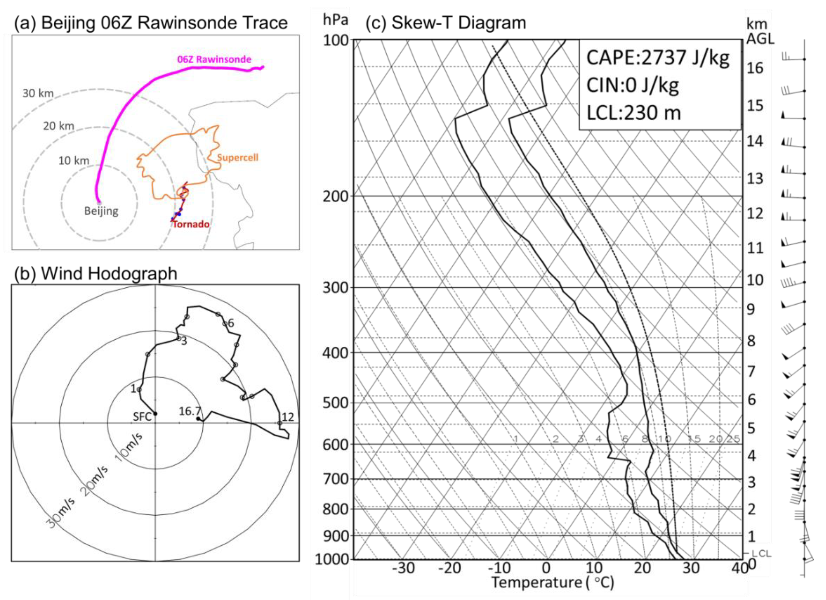
The rawinsonde profile used for the homogeneous initial background was representative of the storm environment in which the tornadic supercell occurred. It was a sounding with 60 layers from the Beijing Meteorological Observatory at 1400 local standard time (LST) (Figure 1), which was initially located 20 km west of the tornado damage path (Figure 1a). It happened to be located in a gap between two convection cells, and thus was not contaminated by convection. The time of the sounding was quite close to the estimated tornado lifetime of ~1340−1400 LST. The radiosonde was around the storm (Figure 1a) and thus providing representative depicting of the storm environment. This sounding in close proximity of the tornadic storm, both spatially and temporally, makes the Beijing tornado case a valuable one for idealized simulation studies. To better represent the near-surface conditions, the surface data of the Beijing radiosonde were modified with the automatic weather station observations from the same location at the same time. The lowest level of the original radiosonde observation is about 30 m above ground level (AGL), while the surface observation is 2 m AGL.

The background environment indicated by the proximity sounding was favorable for severe convective storm development and tornadogenesis. The winds veered with height (Figure 1b) with a 0–6-km vertical shear of 23.4 m s⁻¹ and a 0–1-km vertical shear of 7.1 m s⁻¹, which provides environmental low-level horizontal vorticity required for at least the initial development of mesocyclones. Moreover, convection is easy to initiate and maintain with a high instability characterized by surface-based (which was also the most unstable) convective available potential energy (CAPE) of 2737 J kg⁻¹ and a convection inhibition (CIN) of 0 J kg⁻¹ (Figure 1c). It should be noted that near-surface difference between temperature and dew point temperature is very small, which gives rise to a low lifting condensation level (LCL) of 230 m.

The horizontal grid spacing used in the simulations was 100 m within the central 20 km × 20 km region, and stretched gradually to 3.9 km at the outer boundary (as in [12]) of the 100 km × 100 km domain. The domain moved with the average motion of the simulated supercell, at a constant speed of 2.5 m s⁻¹ eastward and 10 m s⁻¹ northward. The vertical grid spacing was 20 m within the lowest 1 km AGL, and stretched gradually to 500 m at the upper boundary 18 km AGL. A higher resolution was used at lower levels for a better representation of the processes around and below the cloud base. A symmetric ellipsoid warm bubble 20 km wide and 2.8 km deep was added in the initial field, as widely used in previous studies employing idealized simulations. The temperature perturbation was 7 K at its center, located at 1.4 km AGL, and decreasing gradually to zero at its outer edge. The large time step was set as 1 s. A fifth-order advection approximation was used both horizontally and vertically. The Klemp–Wilhelmson time-splitting for acoustic modes was used for the pressure solver, with a vertically implicit solver and horizontally explicit calculations, as in MM5, ARPS and WRF. No topography was considered in this simulation. The explicit moisture scheme used was the Morrison double-moment microphysics scheme with both hail and graupel, which is more realistic in supercell simulation than single-moment schemes. The lateral boundary conditions were set as open radiative, while the bottom boundary condition was free-slip (no friction). The simulation was run for 2 h, with the output saved every 30 s.

The simulations were sensitive to the horizontal and vertical grid spacing. The intensity of the mesocyclone and near-surface vortex decreased with the increase in the horizontal grid spacing from 100 m to 200 m. Increasing the grid spacing to 50 m substantially increased the intensity, but the three-dimensional distribution of the vorticity became complex and lost the key characteristics captured in the 100-m simulation that were close to the observations at both the supercell and tornado scales. The impact of changing the vertical grid spacing was smaller than changing the horizontal grid spacing, but it changed the height of the lowest level and thus the features of the near-surface processes. The configuration used in this study produced a supercell with DRC evolution and tornado intensity variation closest to the observations.

3. Overview of the Simulated Storm

The simulation captured the main features of the supercell structures obtained from radar observations and the tornado characteristics deduced from the damage survey. To compare the simulation and observations more easily, a reference time with respect to tornadogenesis was used. Tornadogenesis was defined as the earliest time when vertical vorticity at the lowest level (10 m AGL) reached 0.1 s⁻¹ and extended from the surface to the cloud base associated with a negative pressure perturbation, as used in the vorticity analysis of a tornado life cycle in Wicker and Wilhelmson [13]. The simulated tornado formed at t = 79 min from the model initiation. This time, along with the estimated time of tornadogenesis in the observations (1340 LST) obtained by MY14, was defined as t₀, and other times are denoted relative to t₀. The location of the Beijing radar in the model was determined based on the relative distance of the Beijing radar from the supercell at t₀ + 4 min of the 2.4° elevation angle scan, to facilitate the visualization of the plan-position-indicator (PPI) view and the calculation of the simulated radial velocities.

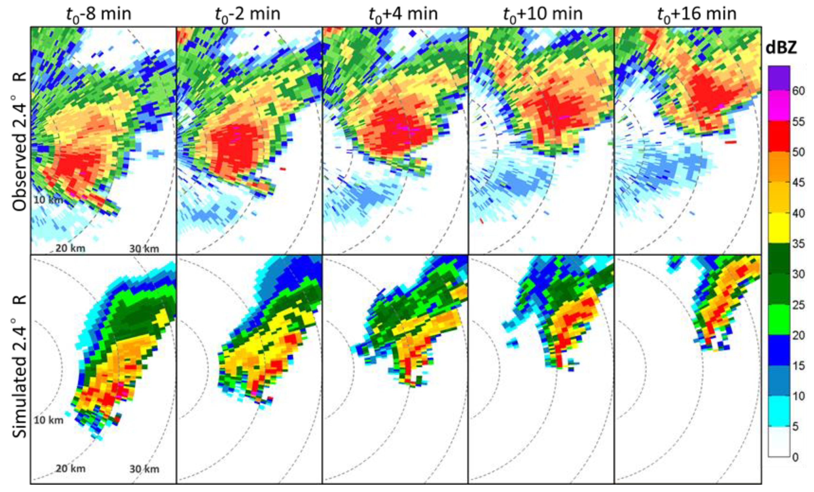
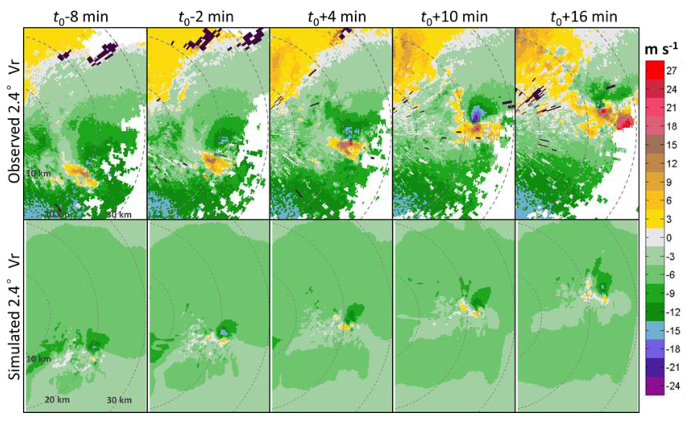
The simulated supercell captured the key features of the observed supercell well in its shape and motion at 2.4° PPI, albeit a smaller size and weaker intensity (Figure 2). The hook echo and weak echo regions observed by radar are also seen in the simulated supercell, which develop and are accompanied by a mesocyclone with a maximum radial velocity somewhat lower than the observed 30 m s⁻¹ (Figure 3). The evolution of a DRC similar to the observations was also captured. Before tornadogenesis, a thin, discrete pillar-shaped DRC was produced with similarity to the radar observation. Since the evolution of the DRC using radar observation is hard to examine due to the limitations in the spatial and temporal resolutions, our simulation provides a valuable dataset for examining how the DRC evolves.

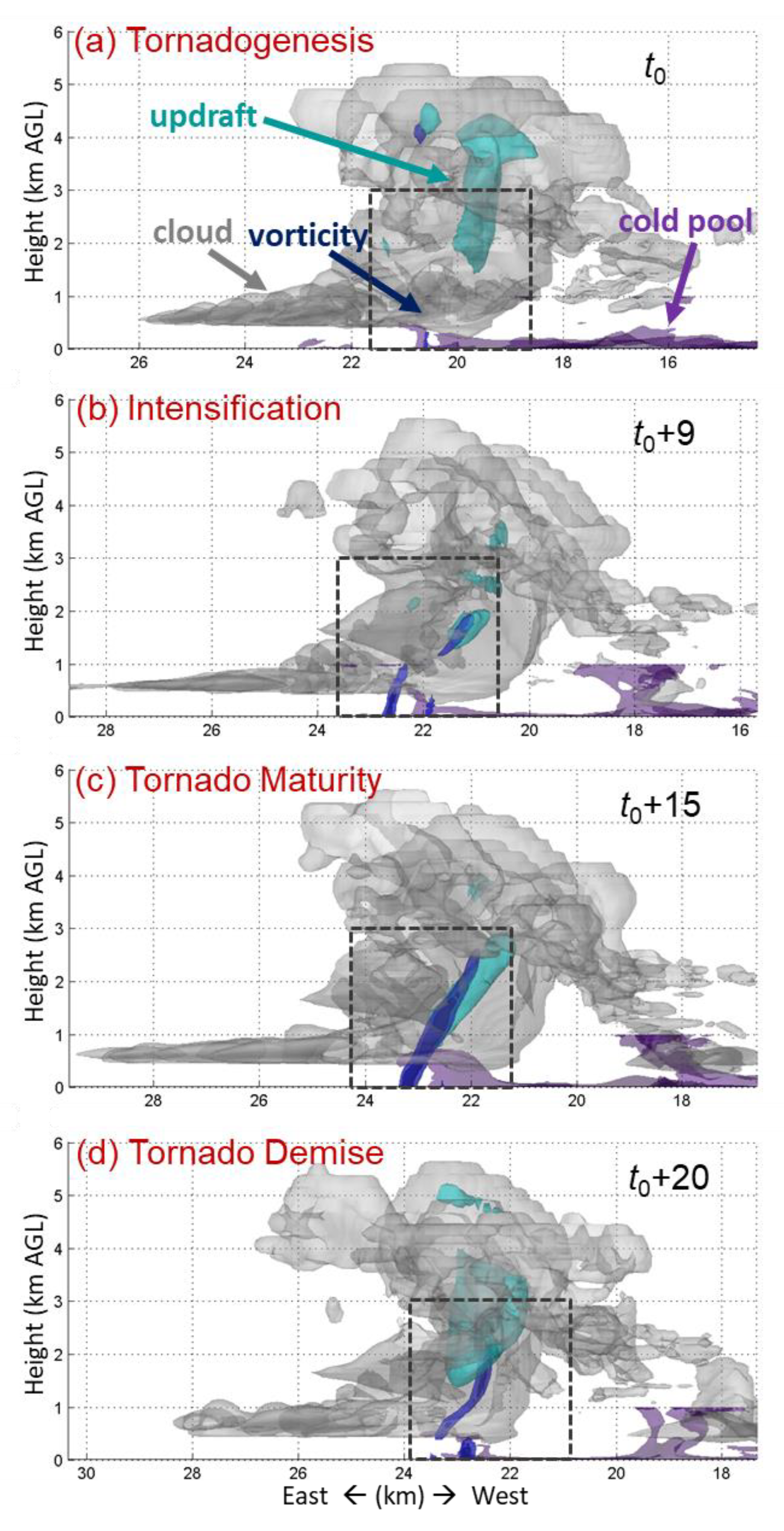
In addition to the supercell, the simulation also shows tornado-scale features with commonalities to the composite information from damage survey and radar observation. The simulated tornado lifespan was 24 min long, similar to the estimated duration of the observed tornado of ~20 min. With composite investigation based on Doppler radar and damage survey, MY14 concluded that this tornado event could be divided into five stages: the formation of the DRC about 16 min before tornadogenesis, the retraction of DRC and the genesis of tornado, the intensification, mature and demise stages of the tornado. This is also the case in the simulation (Figure 4).

The above analyses showed that the cloud model simulated the supercell and tornado reasonably well by using a real radiosonde background. This simulation was therefore used to investigate the evolution of the simulated supercell and tornado, as reported in the next section.

4. Life Cycle of the Simulated Tornado

The model took 27 min to form the supercell from the initial warm bubble. The formation of a supercell was defined as the earliest time when the 2–5-km integrated updraft helicity reached 900 m² s⁻², as introduced by Naylor and Gilmore [6]. After meeting the supercell criteria, the value of 2–5-km integrated updraft helicity oscillated around 900 m² s⁻² for about 15 min and remained greater than 900 m² s⁻² from t = 40 min for the rest of the integration, except for a 10-min oscillation immediately before tornadogenesis. A DRC started to develop at t = 60 min, or 19 min before the tornadogenesis (t₀ − 19 min), and lasted for 17 min. Following the dissipation of the DRC, the tornado was generated at t = 79 min. The tornadogenesis, maintenance (including intensification and maturity) and demise took 4, 13 and 7 min, respectively. These stages are defined by the vertical continuity of the 0.1 s⁻¹ vertical vorticity isosurface columns. There was no sign of more tornadoes after the demise of the tornado. The tornado lasted for 24 min, as measured by the period during which the near-surface vortex column of the 0.1 s⁻¹ vertical vorticity isosurface was sustained, which is similar to the tornado lifetime of about 20 min estimated by MY14.

4.1. DRC Formation (t₀ − 19 min ≤ t < t₀ min)

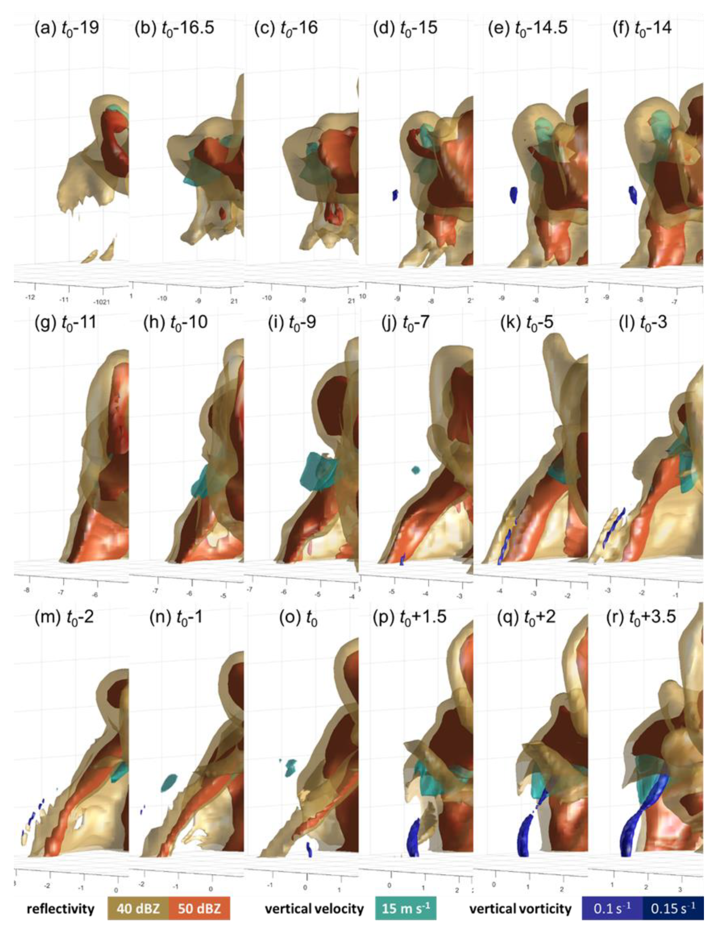
At t₀ − 19 min, an overhanging reflectivity core was first perceivable in terms of the 40-dBZ isosurface (brown in Figure 5a), and later became evident at t₀ − 16 min in terms of the 50-dBZ isosurface at a height of 1.5 km (red in Figure 5b,c). It then expanded while growing rapidly downward and reached the ground at t₀ − 14 min (Figure 5d,f), showing the characteristics of a type I DRC as generalized by Byko et al. [20], which refers to those forming as a result of midlevel flow ‘stagnation’, rather than resulting from precipitation that forms within a new updraft or descended down the axis of an amplifying low-level vertical vorticity maximum. After reaching the ground, the DRC grew wider in the shape of a wall (Figure 5g), then separated into two parts (Figure 5h), gradually forming a pillar of higher reflectivity at its far end (Figure 5i,l), showing the characteristics of a process resembling the 27 May 1997 tornadic supercell case [20], although the latter was not categorized into a typical type as it was not ‘descending’. The high reflectivity pillar became separated from the main body of the supercell and had a diameter of about 500 m, as characterized by the 50-dBZ reflectivity isosurface, extending all the way up to 3 km AGL. Unlike the 50-dBZ isosurface, the 40-dBZ isosurface remained a wall-shaped pattern until t = t₀ − 2.5 min.

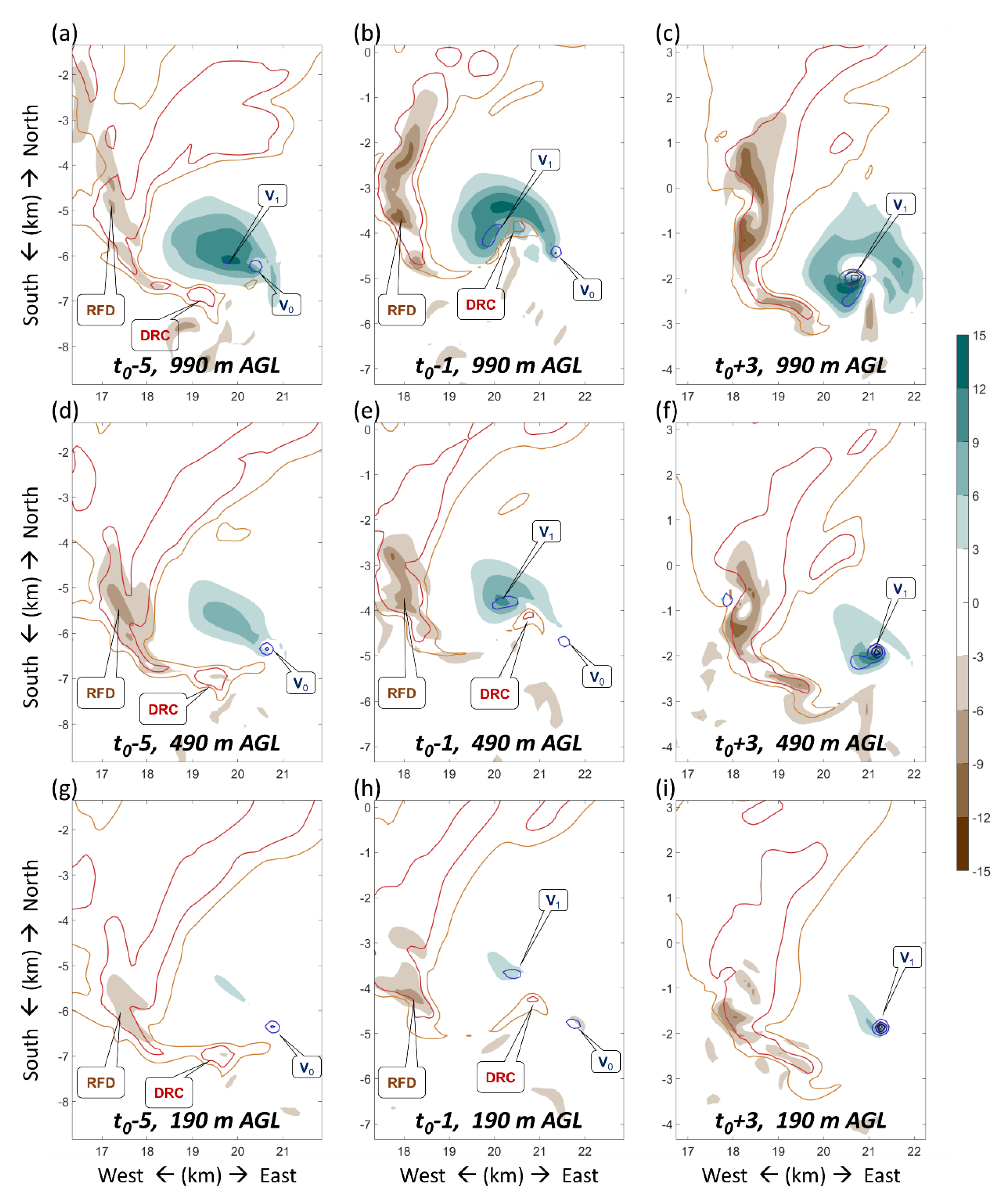
Two minutes after the separation of the DRC from the rear flank downdraft, a weak vertical vorticity column formed near the DRC close to the ground (blue in Figure 5j,k) and attained a strength of 0.1 s⁻¹. This vortex quickly lost contact with the ground and diminished (Figure 5l). The tornadic vortex was not very stable at the earlier stage, with a transient feature. Figure 6 shows that V₀ developed at low-levels from t₀ − 9 min to t₀ − 5 min, which, however, was detached from the main updraft center and hence was not stretched. Later, V₁ developed with a better collocation to the strengthening updraft center throughout the lowest 1-km layers, and hence developed significantly and evolved to become the tornadic vortex.

4.2. Tornadogenesis (t₀ min ≤ t < t₀ + 4 min)

Tornadogenesis was characterized by the newly developed near-surface vortex V₁ at t₀. It happened after the separation of the 40-dBZ isosurface wall of the DRC at t₀ − 2 min, when the previous transient vortex V₀ diminished (Figure 5m). A weak echo hole formed at 500 m AGL and grew larger immediately afterwards, accompanied by a narrowing of the isolated pillar of the DRC in terms of both the 50- and 40-dBZ isosurfaces, with a diameter of about 300 m and 1 km, respectively, at t₀ − 1 min (Figure 5n). Both isosurfaces became thinner and retracted upward approaching tornadogenesis at t₀ and thereafter (Figure 5o–r), and a persistent, vertically upright vortex column near the ground became evident. This retraction of DRC before tornadogenesis was also observed in the radar analysis of MY14. A similar process has also been recorded in the pre-tornadic phase of the 5 June 2009 Goshen County supercell [3].

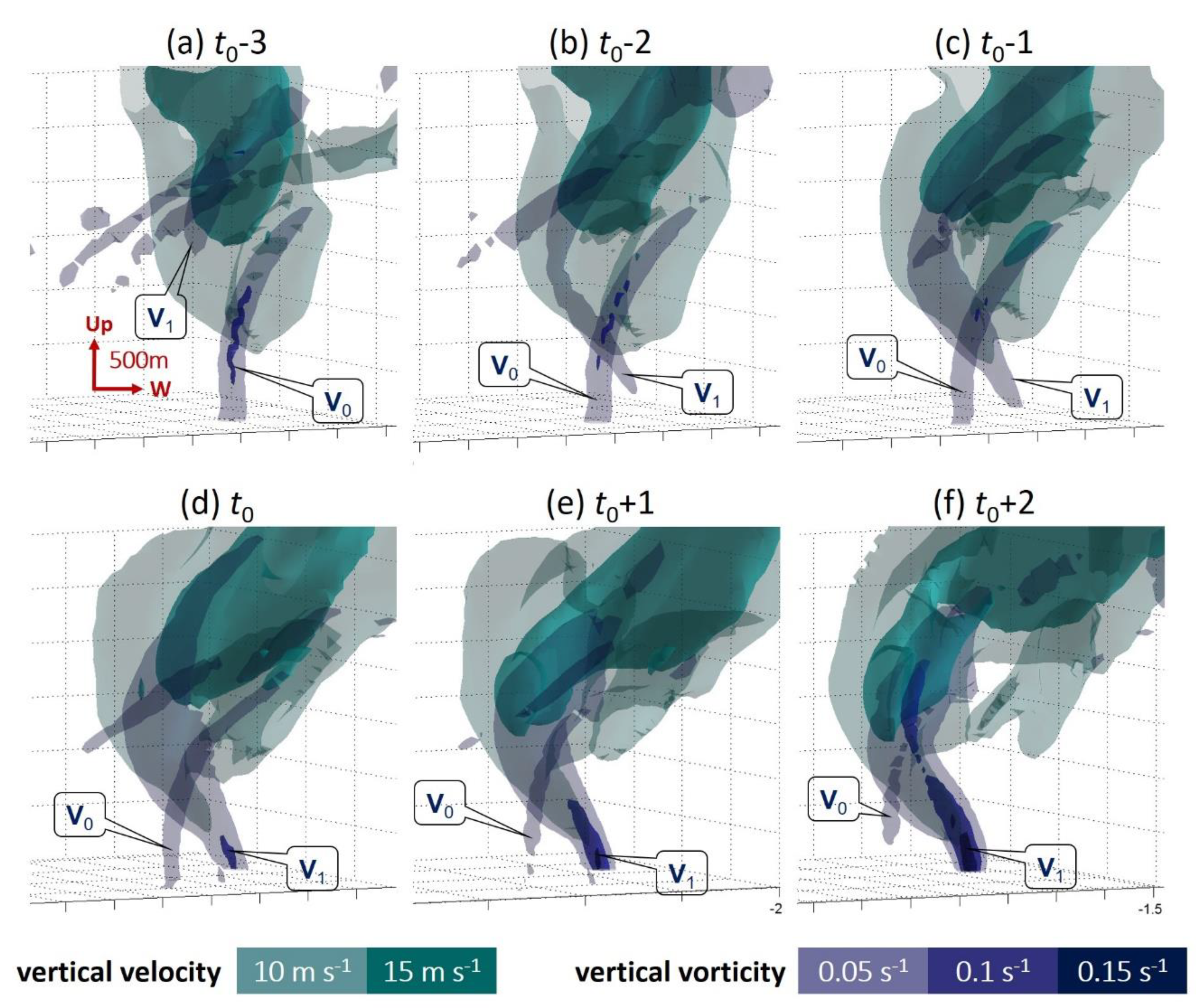
A weak and wide vertical vorticity column, which was likely associated with the mesocyclone, developed downward starting at t₀ – 3 min (denoted by V₁ in Figure 7). About 1 min after the weak and wide vertical vorticity column touched the ground at t₀ − 1 min, the 0.1 s⁻¹ vorticity appeared inside the column near the ground and rapidly developed upward. These analyses showed that the vertical vorticity column was growing in a top-down direction at first, and a stronger vorticity formed inside the column when it was very close to or reached the ground.

The tornadic vortex first formed immediately next to the ground, with a diameter of about 100 m and a height of several hundred meters, connected to the cloud base (Figure 4a). It grew drastically thicker, taller and stronger within 1 min, as indicated by the appearance of 0.15 s⁻¹ vertical vorticity (Figure 8a), which was also connected to the ground at birth. At t₀ + 1.5 min, the DRC pillar disappeared while the tornadic vortex intensified (Figure 5p). During this process, the midlevel updraft also grew lower toward the low-level vortex column (For convenience in describing the results, in terms of the size of the storm, we use ‘midlevel’ to denote levels between 1 and 3 km AGL and ‘low-level’ for those below 1 km AGL.), forming a vorticity column between 1 and 2 km AGL, immediately inside the strong updraft core at t₀ + 2 min (Figure 8a). From t₀ + 2 min onwards, the intensification of the tornadic vortex was also manifested in the intensification of horizontal velocity near the surface. It reached 15 m s⁻¹ near the bottom of the low-level vortex at t₀ + 2 min and expanded in both horizontal and vertical scale. The sequence of mesocyclone, mesocyclone updraft and near-surface tornadic vortex intensification is also observed in the idealized simulations of Roberts et al. [21].

The formation and intensification of the tornadic vortex column was found to be associated with a column of negative pressure perturbation, which resembled a funnel cloud in appearance. At t₀ − 0.5 min, a pressure perturbation of −1.5 hPa was accompanied by a region of 15 m s⁻¹ updraft, both confined to layers above 1 km AGL. With the occurrence of the 0.1 s⁻¹ vertical vorticity column next to the ground, the negative pressure perturbation started to develop downward, and extended to the ground at t₀ + 2 min (Figure 8a, lower row). A stronger perturbation of −2 hPa was embedded inside the −1.5 hPa isosurface, which was between 1 and 2.5 km AGL at t₀ + 0.5 min, and then extended downward to the ground. Opposite to the growth of the tornadic vortex column, which was from the bottom, the pressure perturbation isosurface developed downward from the top, in the same pattern as a tornado funnel cloud. This suggests that tornadogenesis process herein may be further divided into three steps: the downward development of mesocyclone vortex, the upward development of tornado vortex, and the eventual downward development of pressure perturbation and associated condensation of water vapor into cloud water to form the funnel cloud.

The tornado formation first near the ground followed by bottom-up development is consistent with state-of-the-art mobile X-band phase-array radar observations (e.g., [22]) and numerical simulations (e.g., [21,23]), although much earlier observations of TVS based on S-band Doppler radar suggest that the portion of descending and non-descending tornado development is half and half [24]. In our simulation, the downward growth of the vorticity column lasts only about 2 min and thus is likely to be missed by the S-band radar data collected at ~5-minute intervals.

4.3. Tornado Intensification and Maturity (t₀ + 4 min ≤ t < t₀ + 17 min)

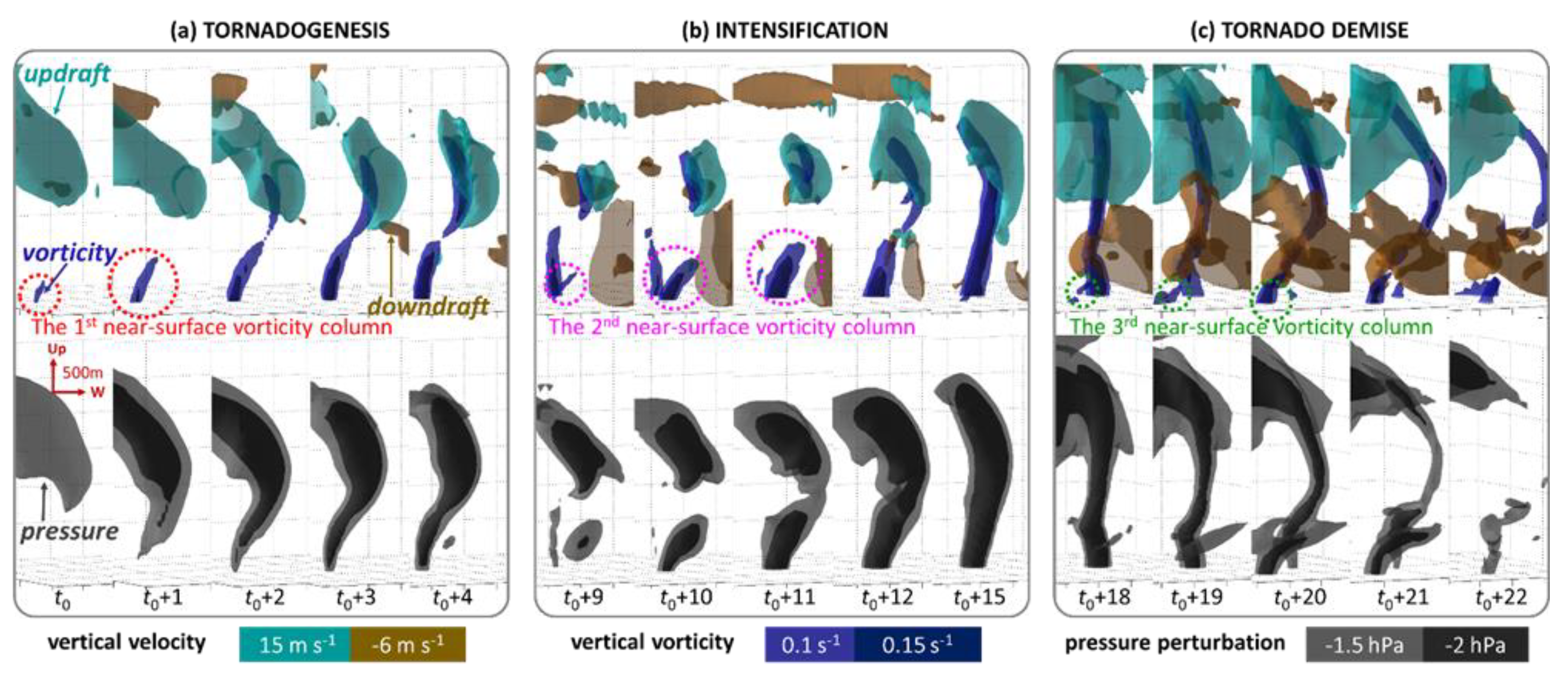
After genesis, the simulated tornadic vortex column experienced a separation and reconnection between the upper and lower vortex column. The 0.1 s⁻¹ vorticity column separated at around 1 km AGL at t₀ + 4 min (Figure 8a). The lower part kept moving outward away from the main supercell while the upper part maintained the same storm-relative location together with the updraft, and shrunk upward. The low-level vortex column was maintained for 10 min (t₀ to t₀ + 10 min). In contrast to the upward retracting dissipation of the weak, thin and short-lived vortex accompanying the DRC formation (Figure 5j–l), this vortex dissipated by retracting downward and staying in contact with the ground, in terms of both the 0.1 and 0.15 s⁻¹ vertical vorticity isosurfaces (Figure 8b).

The separation of the primitive vortex column was not the end of the whole tornado event. Instead, the lower part of the vortex column was replaced by a newly-generated near-surface tornadic vortex (Figure 8b). During this process, the low-level circulation of the tornado vortex decayed while the midlevel vortex remained intact. Then, a new near-surface vortex developed more in line with the midlevel vortex, forming a new surface-based tornado that went on to become stronger. The new vortex was initiated near the ground under the upper part of the vortex column and updraft at t₀ + 9 min (denoted by the magenta dotted ring), and connected to the upper part of the vortex column at t₀ + 12 min. The separation and re-connection process in the variation of the vorticity column also manifested in the variation of the pressure perturbation column, especially in terms of the −2 hPa isosurface (Figure 8b, lower row). The separation of the pressure perturbation isosurface was generally collocated with the separation of the vortex column.

After the replacement of the near-surface tornadic vortex as described above, the tornado reached its maturity. The tornadic vortex became much stronger, such that even the isosurface of 0.15 s⁻¹ vertical vorticity was connected throughout the lowest 2 km depth from t₀ + 14.5 min onwards. The 0.1 s⁻¹ isosurface column expanded to as large as 500 m in diameter. During the mature stage, the top of the whole vorticity column grew gradually higher (Figure 8b), from 2 km AGL to its maximum of over 2.5 km AGL at t₀ + 16.5 min. In terms of the pressure perturbation core, the lower part grew much thicker, with a diameter comparable to its upper part. Coincidentally, the strongest wind of this real tornado event at the ground was produced in this stage, which corresponded to the occurrence of the two fatalities. The wider pressure perturbation and vorticity column might be indicative of the wider damage swath in the Daxinzhuang village, as reported in MY14.

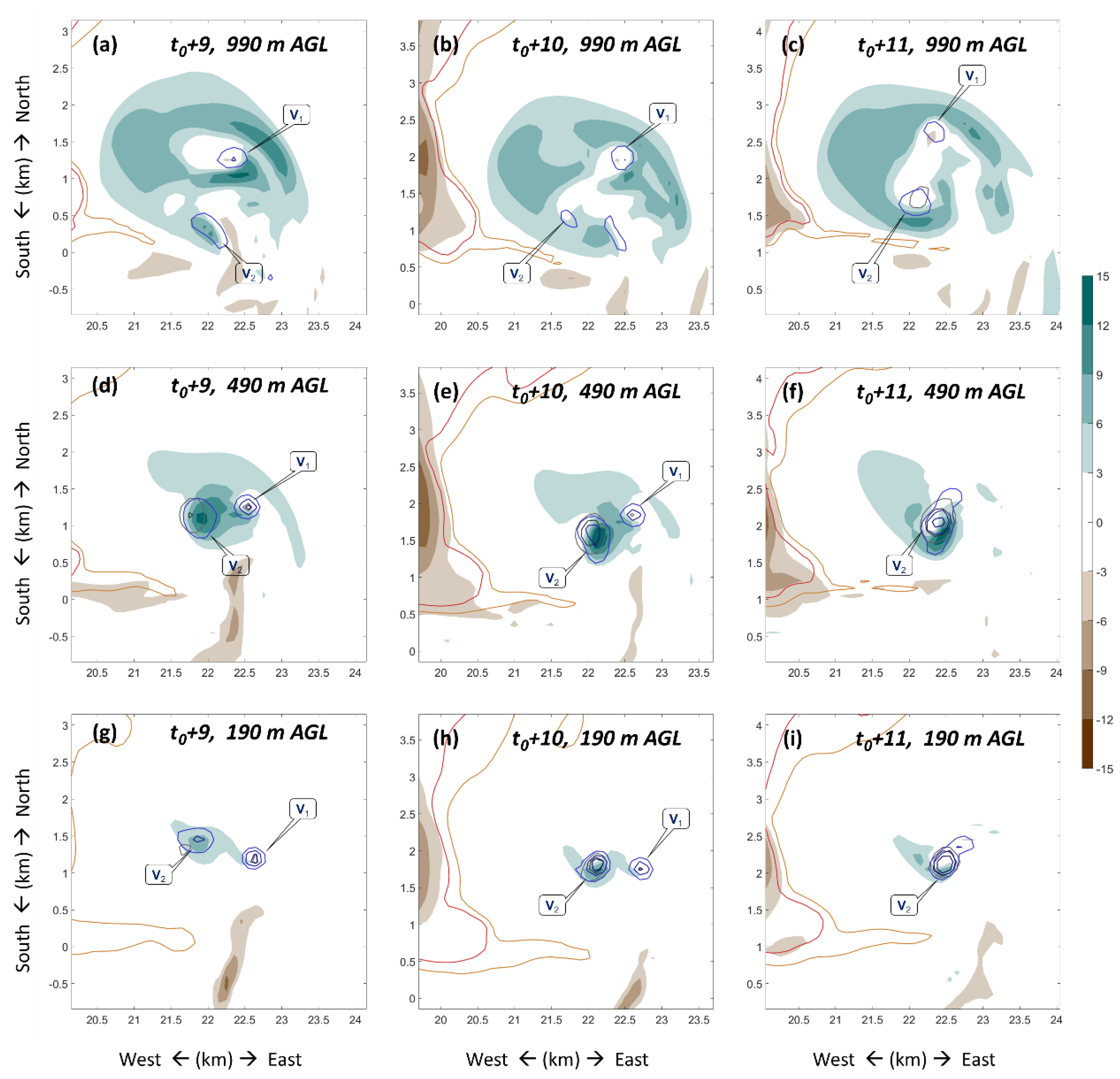
This replacement of the near-surface vortex V₁ by its newly-generated counterpart V₂ was also seen in the horizontal cross-section (Figure 9). Results show that while V₁ weakened due to the detachment from the updraft center, V₂ intensified with the stretching by the strong updraft center. The three-dimensional isosurface helps to depict the general structure of the spiral nature of the tornadic vortices, while the two-dimensional contour plots provide more precise details. This indicates that a combination of these two illustration methods may be more suitable for tornado structure analysis.

The vortex replacement process is similar to the cyclic mesocyclogenesis in numerical simulation by Adlerman et al. [25] and tornadogenesis in radar observation by Dowell and Bluestein [26]. The key difference is that the replacement in our simulation happened mainly for the near-surface vortices with the midlevel mesocyclone remaining the same. The former near-surface tornadic vortex was detached from the updraft center while the newly-generated vortex was connected to and stretched by the same midlevel mesocyclone. However, in Adlerman et al. [25] the replacement happened mainly to the midlevel mesocyclones rather than the near-surface vortices.

4.4. Tornado’s Demise (t₀ + 17 min ≤ t ≤ t₀ + 24 min)

The tornado’s demise occurred in association with another separation in the vorticity and pressure perturbation columns. Early on at t₀ + 15 min, a new surface-based vorticity column developed near the bottom of the main one (Figure 8b), similar to the previous separation and reconnection process. However, the evolution of the vorticity and pressure perturbation associated with the vortex was different from the previous cycle. Instead of a sharp separation, the columns bent around the 1.5 km AGL layer (t₀ + 20 min, Figure 8c) while becoming thinner. The final separation occurred at about t₀ + 20 min below 500 m AGL. Though the new tornadic vortex column grew thicker, it was not able to connect to the upper part of the storm. No strong horizontal wind accompanied it either. The near-surface vortex column died out rapidly, with a height confined to no more than 500 m. The upper part separated into several parts and died out as well, when it bent outward and was detached from the rotational updraft. The whole process looked quite similar to the disappearance of a funnel cloud (sometimes in a rope shape).

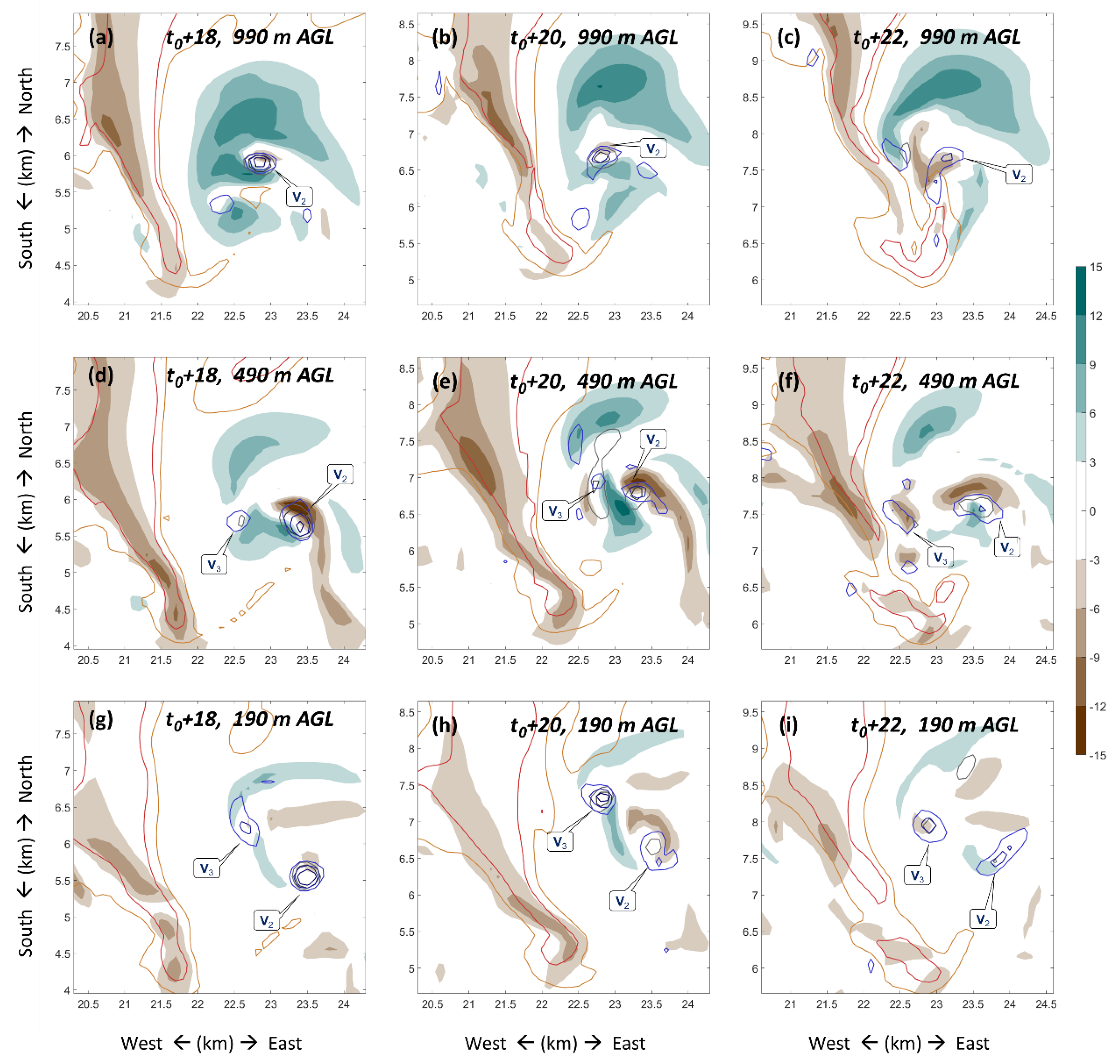
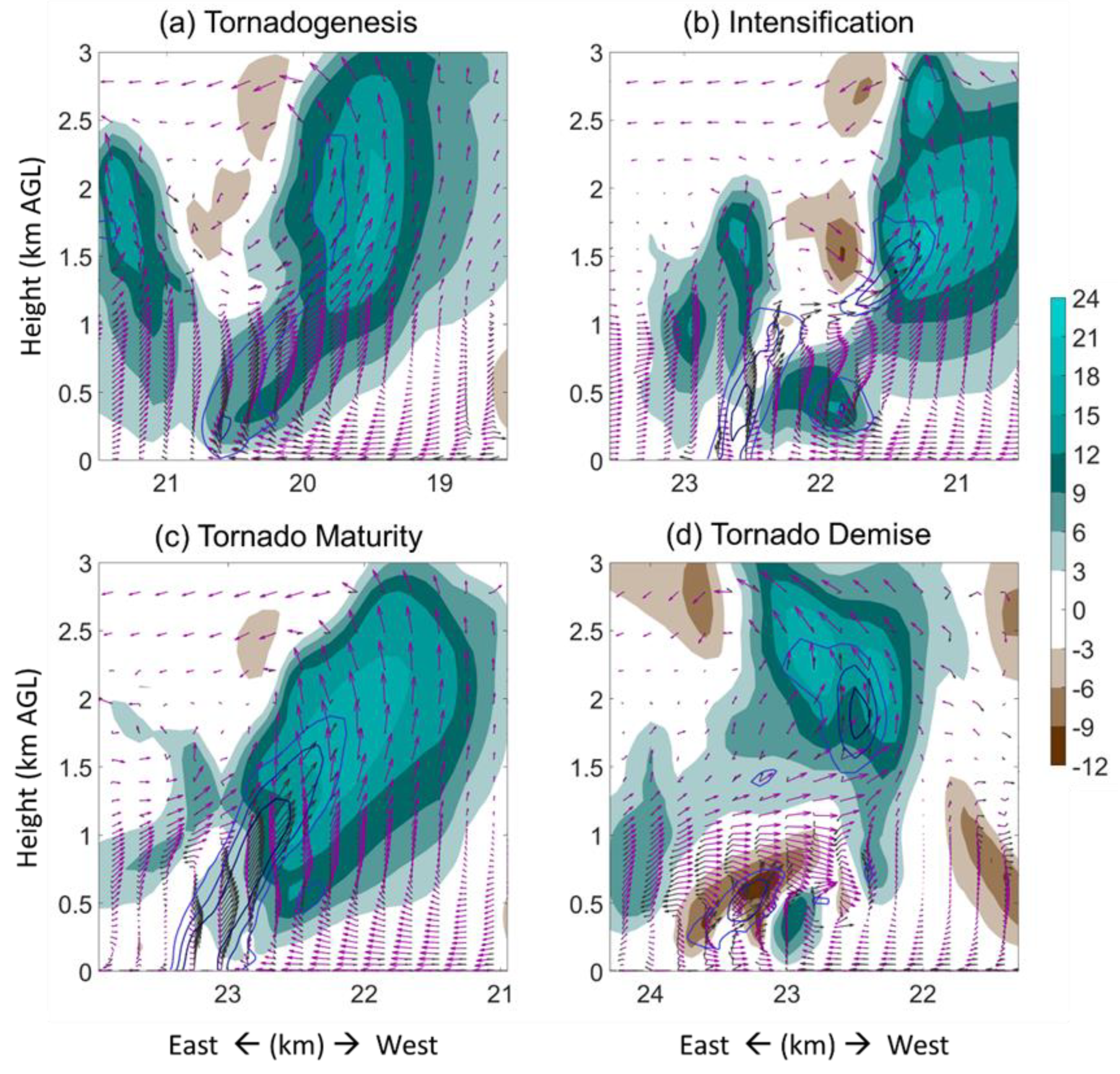
The bending of the upper vortex and the failure of the reconnection between the new near-surface vortex and midlevel mesocyclone were associated with a developing downdraft (brown in Figure 8c). At this stage, updraft at low levels was greatly distorted by the intrusion of downdraft (Figure 10). Although another newly-generated near-surface vortex V₃ strengthened at around t₀ + 20 min, neither V₃ nor V₂ was steadily stretched by the updraft, which was maintained above a 1 km AGL layer (Figure 10a–c), but weakened significantly at low levels (Figure 10d–i). From vertical cross-section, the low-level vortex was ‘capped’ by strong downward wind field (Figure 11d), prohibiting the stretching of the low-level rotation from midlevel updraft. By contrast, the near-surface vortices were accompanied by steady continuous updrafts at early stages (Figure 11a–c). There is also a downdraft presented at midlevel associated with the short-term weakening during the intensification stage, which might have been the cause for the first replacement of the near-surface tornado vortex. The formation mechanism of these downdrafts is beyond the scope of this paper, and will be studied separately.

The supercell weakened after the tornado’s demise. At the end of simulation (t = 120 min, or t₀ + 41 min, not shown), the storm remained a supercell, with a 2–5-km updraft helicity of ~1300 m² s⁻² and a bounded weak echo region.

5. Summary and Discussion

Based on an idealized cloud model simulation using an observed proximity sounding of the 21 July 2012 Beijing tornadic supercell and warm bubble storm initiations, the simulated supercell and tornado reasonably captured the main features observed by the Beijing operational S-band Doppler radar. From the simulation, detailed evolution of the storm and embedded tornado from their formation to demise was examined.

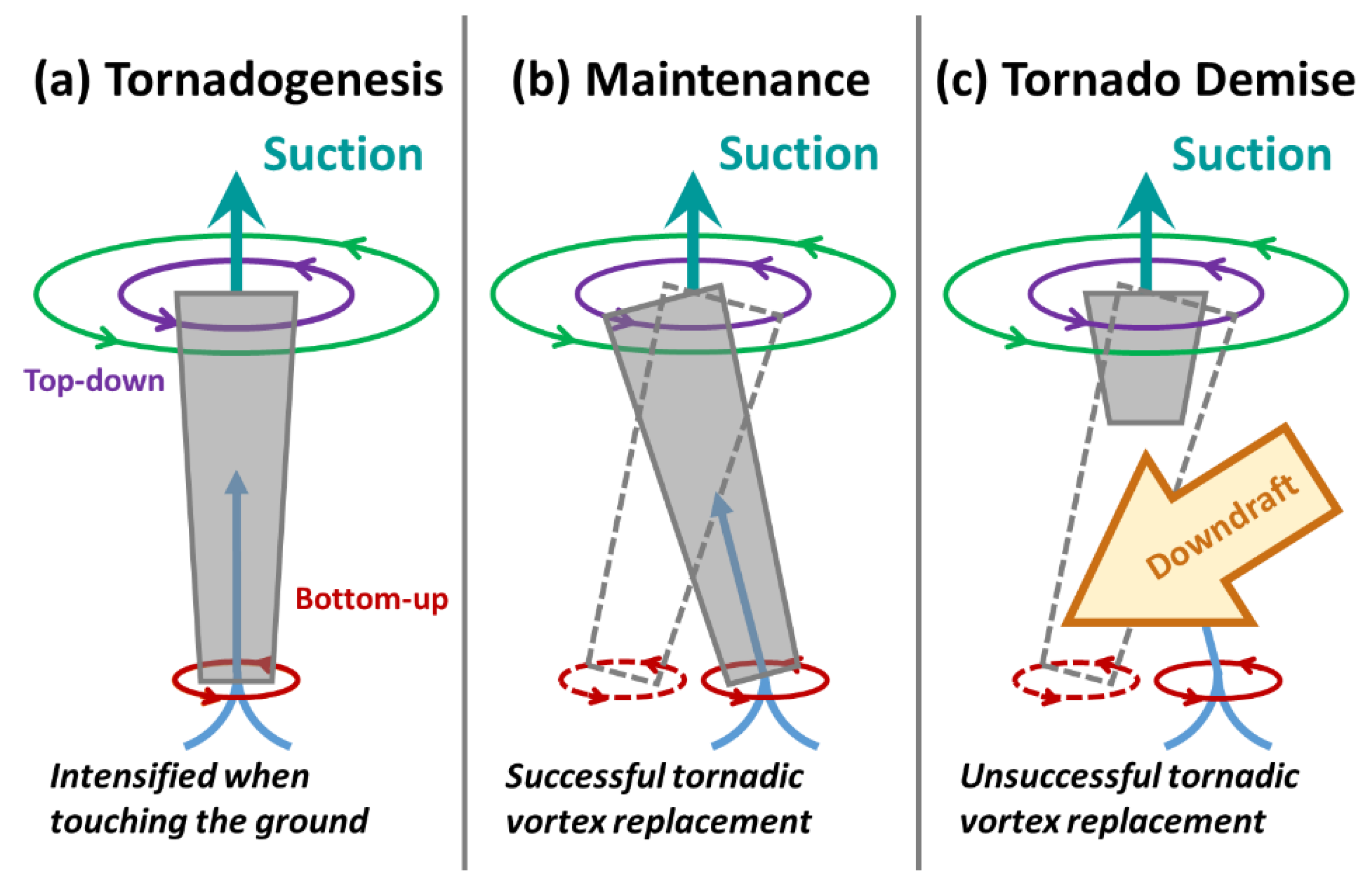
The details of the DRC and the sequence of events leading up to tornadogenesis and throughout the evolution of tornado were examined, including downward development of mesocyclone vortex, the upward development of tornado vortex, and the eventual downward development of condensation funnel cloud. The simulation revealed a DRC evolution that had commonalities with the radar observation of this tornado event. The DRC formed about 17 min before the tornadogenesis, which retracted upward immediately before tornadogenesis, similar to radar observations. The tornado formed through downward development of the mesocyclone towards the ground, followed by the rapid upward growth of the tornado-scale vortex underneath the mesocyclone (Figure 12a). This bottom-up development provides a numerical evidence for the growing support for a bottom-up, rapid tornadogenesis process as revealed by the state-of-the-art mobile X-band phase-array radar observations and is also consistent with most recent simulation studies.

During the tornado intensification stage, the modeled tornadic vortex experienced a vertical separation and a reconnection between the upper vortex and a newly developed near-surface vortex (Figure 12b). The tornado’s demise came about when another round of vortex column separation occurred. Even though a new near-surface vortex appeared underneath the midlevel mesocyclone, stretching was prohibited by the development of downdraft over the near-surface vorticity, and the tornado eventually collapsed (Figure 12c). The key process leading to the maintenance and demise processes herein calls for proper alignment between midlevel mesocyclone and low-level tornadic vortices, which generally agrees with suggestions from previous studies [12,27]. One uniqueness of this result is that the tornado vortex cycling could be a replacement of the near-surface vortices while the midlevel mesocyclone remains the same. Moreover, our analyses here emphasize the role of downdraft intruding on the tornado vortex as a cause of tornado demise.

In order to obtain the simulation reported in this study that shares many commonalities with observations, we performed many sensitivity experiments beforehand. We found that tornadic features were highly sensitive to model configurations. Furthermore, the large warm bubble strength of 7 K needed to initiate a sustained tornadic storm suggests that some features of the observed sounding, such as the relatively warm mid-levels, of this case may not be most favorable for most intense supercell storm. Even higher spatial resolutions, the inclusion of mesoscale forcing in horizontally inhomogeneous initial conditions, as well as the inclusion of surface friction may be needed to obtain even more realistic simulations. The absence of surface friction as another source of near-surface vorticity may be an important reason of the weaker than observed tornado vortices obtained, as advocated by recent studies (e.g., [11,21,28]). These can be topics for future studies.

References

- Pazmany, A.L.; Mead, J.B.; Bluestein, H.B.; Snyder, J.C.; Houser, J.B. A mobile rapid-scanning x-band polarimetric (RaXPol) Doppler radar system. J. Appl. Meteor. 2013, 30, 1398–1413. [Google Scholar] [CrossRef]
- Houser, J.L.; Bluestein, H.B.; Snyder, J.C. A finescale radar examination of the tornadic debris signature and weak-echo reflectivity band associated with a large, violent tornado. Mon. Wea. Rev. 2016, 144, 4101–4130. [Google Scholar] [CrossRef]
- Markowski, P.; Richardson, Y.; Marquis, J.; Wurman, J.; Kosiba, K.; Robinson, P.; Rasmussen, E.; Dowell, D. The Pretornadic Phase of the Goshen County, Wyoming, Supercell of 5 June 2009 Intercepted by VORTEX2. Part II: Intensification of Low-Level Rotation. Mon. Wea. Rev. 2012, 140, 2916–2938. [Google Scholar] [CrossRef]
- Marquis, J.; Richardson, Y.; Markowski, P.; Wurman, J.; Kosiba, K.; Robinson, P. An Investigation of the Goshen County, Wyoming, Tornadic Supercell of 5 June 2009 Using EnKF Assimilation of Mobile Mesonet and Radar Observations Collected during VORTEX2. Part II: Mesocyclone-Scale Processes Affecting Tornado Formation, Maintenance, and Decay. Mon. Wea. Rev. 2016, 144, 3441–3463. [Google Scholar]
- Clark, A.J.; Gao, J.; Marsh, P.T.; Smith, T.; Kain, J.S.; Correia, J., Jr.; Xue, M.; Kong, F. Tornado Pathlength Forecasts from 2010 to 2011 Using Ensemble Updraft Helicity. Wea. Forecasting. 2013, 28, 387–407. [Google Scholar] [CrossRef]
- Naylor, J.; Gilmore, M.S. Vorticity Evolution Leading to Tornadogenesis and Tornadogenesis Failure in Simulated Supercells. J. Atmos. Sci. 2014, 71, 1201–1217. [Google Scholar] [CrossRef]
- Stensrud, D.J.; Wicker, L.J.; Xue, M.; Dawson, D.T.; Yussouf, N.; Wheatley, D.M.; Thompson, T.E.; Snook, N.A.; Smith, T.M.; Schenkman, A.D.; et al. Progress and challenges with Warn-on-Forecast. Atmospheric Research. 2013, 123, 2–16. [Google Scholar] [Green Version]
- Xue, M.; Hu, M.; Schenkman, A.D. Numerical Prediction of the 8 May 2003 Oklahoma City Tornadic Supercell and Embedded Tornado Using ARPS with the Assimilation of WSR-88D Data. Wea. Forecasting. 2014, 29, 39–62. [Google Scholar] [CrossRef]
- Mashiko, W. A Numerical Study of the 6 May 2012 Tsukuba City Supercell Tornado. Part I: Vorticity Sources of Low-Level and Midlevel Mesocyclones. Mon. Wea. Rev. 2016, 144, 1069–1092. [Google Scholar] [CrossRef]
- Mashiko, W. A Numerical Study of the 6 May 2012 Tsukuba City Supercell Tornado. Part II: Mechanisms of Tornadogenesis. Mon. Wea. Rev. 2016, 144, 3077–3098. [Google Scholar] [CrossRef]
- Schenkman, A.D.; Xue, M.; Hu, M. Tornadogenesis in a High-Resolution Simulation of the 8 May 2003 Oklahoma City Supercell. J. Atmos. Sci. 2014, 71, 130–154. [Google Scholar] [CrossRef]
- Markowski, P.M.; Richardson, Y.P. The Influence of Environmental Low-Level Shear and Cold Pools on Tornadogenesis: Insights from Idealized Simulations. J. Atmos. Sci. 2014, 71, 243–275. [Google Scholar] [CrossRef]
- Wicker, L.J.; Wilhelmson, R.B. Simulation and Analysis of Tornado Development and Decay within a Three-Dimensional Supercell Thunderstorm. J. Atmos. Sci. 1995, 52, 2675–2703. [Google Scholar] [CrossRef] [Green Version]
- Wilhelmson, R.B.; Klemp, J.B. A Three-Dimensional Numerical Simulation of Splitting Severe Storms on 3 April 1964. J. Atmos. Sci. 1981, 38, 1581–1600. [Google Scholar] [CrossRef] [Green Version]
- Klemp, J.B.; Wilhelmson, R.B.; Ray, P.S. Observed and Numerically Simulated Structure of a Mature Supercell Thunderstorm. J. Atmos. Sci. 1981, 38, 1558–1580. [Google Scholar] [CrossRef] [Green Version]
- Klemp, J.B.; Rotunno, R. A Study of the Tornadic Region within a Supercell Thunderstorm. J. Atmos. Sci. 1983, 40, 359–377. [Google Scholar] [CrossRef] [Green Version]
- Orf, L.; Wilhelmson, R.; Lee, B.; Finley, C.; Houston, A. Evolution of a Long-Track Violent Tornado within a Simulated Supercell. Bull. Amer. Meteorol. Soc. 2017, 98, 45–68. [Google Scholar] [CrossRef]
- Meng, Z.; Yao, D. Damage Survey, Radar, and Environment Analyses on the First-Ever Documented Tornado in Beijing during the Heavy Rainfall Event of 21 July 2012. Wea. Forecasting. 2014, 29, 702–724. [Google Scholar] [CrossRef]
- Bryan, G.H.; Fritsch, J.M. A Benchmark Simulation for Moist Nonhydrostatic Numerical Models. Mon. Wea. Rev. 2002, 130, 2917–2928. [Google Scholar] [CrossRef]
- Byko, Z.; Markowski, P.; Richardson, Y.; Wurman, J.; Adlerman, E. Descending Reflectivity Cores in Supercell Thunderstorms Observed by Mobile Radars and in a High-Resolution Numerical Simulation. Wea. Forecasting. 2009, 24, 155–186. [Google Scholar] [CrossRef]
- Roberts, B.; Xue, M.; Schenkman, A.D.; Dawson, D.T. The role of surface friction in tornadogenesis within an idealized supercell simulation. J. Atmos. Sci., 2016, 73, 3371–3395. [Google Scholar] [CrossRef]
- French, M.M.; Bluestein, H.B.; PopStefanija, I.; Baldi, C.A.; Bluth, R.T. Reexamining the Vertical Development of Tornadic Vortex Signatures in Supercells. Mon. Wea. Rev. 2013, 141, 4576–4601. [Google Scholar] [CrossRef]
- Yao, D.; Xue, H.; Yin, J.; Sun, J.; Liang, X.; Guo, J. Investigation into the Formation, Structure, and Evolution of an EF4 Tornado in East China Using a High-Resolution Numerical Simulation. J. Meteorol. Res. 2018, 32, 157–171. [Google Scholar] [CrossRef]
- Trapp, R.J.; Mitchell, E.D.; Tipton, G.A.; Effertz, D.W.; Watson, A.I.; Andra, D.L.; Magsig, M.A. Descending and Nondescending Tornadic Vortex Signatures Detected by WSR-88Ds. Wea. Forecasting. 1999, 14, 625–639. [Google Scholar] [CrossRef]
- Adlerman, E.J.; Droegemeier, K.K.; Davies-Jones, R. A Numerical Simulation of Cyclic Mesocyclogenesis. J. Atmos. Sci. 1999, 56, 2045–2069. [Google Scholar] [CrossRef]
- Dowell, D.C.; Bluestein, H.B. The 8 June 1995 McLean, Texas, Storm. Part I: Observations of Cyclic Tornadogenesis. Mon. Wea. Rev. 2002, 130, 2626–2648. [Google Scholar] [CrossRef]
- Snook, N.; Xue, M. Effects of Microphysical Drop Size Distribution on Tornadogenesis in Supercell Thunderstorms. Geophys. Res. Lett. 2008, 35, 851–854. [Google Scholar] [CrossRef]
- Roberts, B.; Xue, M. The role of surface drag in mesocyclone intensification leading to tornadogenesis within an idealized supercell simulation. J. Atmos. Sci., 2017, 74, 3055–3077. [Google Scholar] [CrossRef]
Figure 1.
Beijing weather station rawinsonde in close proximity to the Beijing tornado at 0600 UTC (1400 LST, which was launched at 1315 LST) on 21 July 2012. (a) Spatial proximity of the rawinsonde trace (magenta curve) to the supercell (denoted by the contour of 45 dBZ at 2.4° elevation angle at 1350 LST) and the tornado track (in red, adapted from MY14). The blue dots show the seven affected villages. The grey curve is the eastern border of Beijing. The Beijing weather station is denoted by the grey dot and the distance scale is given by concentric grey dashed circles. (b) Hodograph of the Beijing rawinsonde, with the altitudes (km) of different levels given alongside the curve. (c) Vertical profiles of temperature, dew point and wind from the rawinsonde in a Skew-T diagram. Also shown are the values of CAPE, CIN and LCL.
Figure 2.
Two-dimensional comparison between observed (upper row) and simulated (lower row) supercells in terms of basic reflectivity (R) at 2.4° elevation angle contours at five scanning times. The ranges at 10, 20 and 30 km are given by concentric circles centered on the radar site.
Figure 3.
As in Figure 2 but for radial velocity (Vr).
Figure 4.
Three-dimensional perspective of the simulated tornado and cumulonimbus cloud at the (a) tornadogenesis, (b) intensification, (c) maturity and (d) demise stages. The isosurfaces in grey, cyan, blue and purple denote the cloud water vapor mixing ratio (0.1 g kg−1), vertical velocity (15 m s−1), vertical vorticity (0.1 s−1) and potential temperature perturbation (−1 K, showing the temperature properties of the cold pool), respectively. The perspective is from the north.
Figure 5.
Simulated three-dimensional supercell structure in terms of reflectivity, vertical velocity and vertical vorticity from (a) t0 – 19 min to (r) t0 + 3.5 min at specific times as denoted. The tornadic supercell is during the period of DRC formation and tornadogenesis. The isosurfaces of 0.1 s−1 and 0.15 s−1 vertical vorticity are given in dark blue. The updraft of the mesocyclone of 15 m s−1 is shown in cyan. The isosurfaces of 40 and 50 dBZ reflectivity are given in brown and red, respectively.
Figure 6.
Horizontal cross-section of the simulated supercell and tornado during DRC formation and tornadogenesis at the height of (a−c) 990 m, (d−f) 490 m and (g−i) 190 m AGL at (left column) t0 − 5 min, (middle column) t0 − 1 min and (right column) t0 + 3 min. Vertical velocity is given by shaded contours. Reflectivity of 40 (50) dBZ is given by orange (red) contours. Vertical vorticity of 0.05, 0.1 and 0.15 s−1 is given by blue contours. Pressure perturbation of -1.5 and -2 hPa is given by dark grey contours. V0 denotes the vanishing vortex associated with the DRC, while V1 denotes the downward developing tornadic vortex.
Figure 7.
Evolution of vertical vorticity column near the tornadogenesis period from (a) t0 − 3 min to (f) t0 + 2 min at an interval of 1 min. Cyan and light cyan denote the 15 and 10 m s−1 vertical velocity, respectively. The dark blue to transparent dark blue denote the 0.15, 0.1 and 0.05 s−1 vertical vorticity, respectively. The distance scales in the vertical and horizontal directions are given in (a). V0 denotes the vanishing vortex associated with the DRC, while V1 denotes the downward developing tornadic vortex.
Figure 8.
Structure and development of rotational column (upper row) versus pressure perturbation core (lower row) during stages of (a) tornadogenesis, (b) intensification and (c) demise. The isosurface of 0.1 s−1 vertical vorticity is given in dark blue, embedded with a darker blue isosurface denoting 0.15 s−1. The updraft of the mesocyclone of 15 m s−1 is shown in cyan, while the downdraft of −6 m s−1 is in brown. The dark grey and black isosurfaces in the lower row depict the pressure perturbation of −1.5 and −2 hPa, respectively. The distance scales in the vertical and horizontal directions are given in (a).
Figure 9.
Horizontal cross-section of the simulated supercell and tornado in the first near-surface vorticity replacement during the tornado intensification stage at the height of (a−c) 990 m, (d−f) 490 m and (g−i) 190 m AGL at (left column) t0 + 9 min, (middle column) t0 + 10 min and (right column) t0 + 11 min. Vertical velocity is given by shaded contours. Reflectivity of 40 (50) dBZ is given by orange (red) contours. Vertical vorticity of 0.05, 0.1 and 0.15 s−1 is given by blue contours. Pressure perturbation of−1.5 and −2 hPa is given by dark grey contours. V1 and V2 denote the first and second tornadic vortices, respectively.
Figure 10.
Horizontal cross-section of the simulated supercell and tornado in the second near-surface vorticity replacement during the tornado demise stage at the height of (a−c) 990 m, (d−f) 490 m and (g−i) 190 m AGL at (left column) t0 + 18 min, (middle column) t0 + 20 min and (right column) t0 + 22 min. Vertical velocity is given by shaded contours. Reflectivity of 40 (50) dBZ is given by orange (red) contours. Vertical vorticity of 0.05, 0.1 and 0.15 s−1 is given by blue contours. Pressure perturbation of −1.5 and −2 hPa is given by dark grey contours. V2 and V3 denote the second and third tornadic vortices, respectively.
Figure 11.
Vertical cross-section of the simulated supercell and tornado during the tornado lifecycle at range indicated by boxes in Figure 4, at the (a) tornadogenesis, (b) intensification, (c) maturity and (d) demise stages. Vertical velocity is given by shaded contours. Vertical vorticity of 0.05, 0.1 and 0.15 s−1 is given by blue contours. Wind (vorticity) field is given by magenta (black) vectors.
Figure 12.
Schematic diagrams of the (a) genesis, (b) maintenance and (c) demise processes of the Beijing tornado event based on the idealized simulation. The suction and circulation of the midlevel mesocyclone are denoted by the cyan arrow and green circle, respectively. The circulation of the enhanced moderate rotation of the midlevel mesocyclone is denoted in purple, which develops top-down toward the ground. The stronger rotation at the ground is denoted by red circles. Blue arrows denote the stretching of the near-surface tornadic vortices. The grey column denotes the tornado funnel cloud. The dashed lines in (b) and (c) denote the weakened former tornado column. The brown arrow in (c) denotes the strengthened downdraft that cuts off the connection between the newly developed near-surface tornadic vortex and the suction of the midlevel mesocyclone.
© 2019 by the authors. Licensee MDPI, Basel, Switzerland. This article is an open access article distributed under the terms and conditions of the Creative Commons Attribution (CC BY) license (http://creativecommons.org/licenses/by/4.0/).
Share and Cite
MDPI and ACS Style
Yao, D.; Meng, Z.; Xue, M. Genesis, Maintenance and Demise of a Simulated Tornado and the Evolution of Its Preceding Descending Reflectivity Core (DRC). Atmosphere 2019, 10, 236. https://doi.org/10.3390/atmos10050236
AMA Style
Yao D, Meng Z, Xue M. Genesis, Maintenance and Demise of a Simulated Tornado and the Evolution of Its Preceding Descending Reflectivity Core (DRC). Atmosphere. 2019; 10(5):236. https://doi.org/10.3390/atmos10050236
Chicago/Turabian StyleYao, Dan, Zhiyong Meng, and Ming Xue. 2019. "Genesis, Maintenance and Demise of a Simulated Tornado and the Evolution of Its Preceding Descending Reflectivity Core (DRC)" Atmosphere 10, no. 5: 236. https://doi.org/10.3390/atmos10050236
Note that from the first issue of 2016, this journal uses article numbers instead of page numbers. See further details here.