Crossing Multiple Gray Zones in the Transition from Mesoscale to Microscale Simulation over Complex Terrain

Abstract

This review paper explores the field of mesoscale to microscale modeling over complex terrain as it traverses multiple so-called gray zones. In an attempt to bridge the gap between previous large-scale and small-scale modeling efforts, atmospheric simulations are being run at an unprecedented range of resolutions. The gray zone is the range of grid resolutions where particular features are neither subgrid nor fully resolved, but rather are partially resolved. The definition of a gray zone depends strongly on the feature being represented and its relationship to the model resolution. This paper explores three gray zones relevant to simulations over complex terrain: turbulence, convection, and topography. Taken together, these may be referred to as the gray continuum. The focus is on horizontal grid resolutions from ∼10 km to ∼10 m. In each case, the challenges are presented together with recent progress in the literature. A common theme is to address cross-scale interaction and scale-awareness in parameterization schemes. How numerical models are designed to cross these gray zones is critical to complex terrain applications in numerical weather prediction, wind resource forecasting, and regional climate modeling, among others.

1. Introduction

Atmospheric models are becoming an indispensable source of knowledge about our planet’s current and future state. In addition to predicting daily changes in weather, numerical models are used to drive air quality models, to provide wind resource assessments, and to predict long-term climate such as spatial and temporal changes in weather patterns. These forecasts play a critical role in everyday life, affecting economic, personal, and environmental decisions among others [1].

Most of these atmospheric predictions are made over complex terrain, where topography and land-use heterogeneity directly impact the evolution of the atmosphere. The influence of complex terrain can drive local circulations (e.g., thermally-driven winds [2]) or regional scale flow (e.g., upstream blocking from mountain ranges [3]). Lehner and Rotach [4] reviewed many of these mountain transport and exchange processes, including gravity waves and moist convection. For numerical models, complex terrain poses a number of challenges. First, accurately representing turbulent processes is essential to models at all scales, to properly dissipate kinetic energy and represent mixing in the atmosphere. The influence of complex terrain on turbulence parameterizations must also be considered. Second, the parameterization of convective processes is required at coarser resolutions, and is impacted by orographic triggering of convection over complex terrain. This is difficult to capture because local moisture and temperature fields are strongly modulated by mountain circulations. Finally, the accurate representation of topography is critical, yet is limited over steep terrain by choices in the underlying numerical grid representation.

In all of these areas, there are unique challenges posed by the transition from mesoscale to microscale modeling regimes and the gray zones encountered in the process of moving across resolutions. The gray zone here refers to the challenge of transitioning from parameterization of physical processes to explicit resolution of these processes as the grid is refined [5,6]. (In the context of turbulence modeling, the gray zone is often called the terra incognita, a phrase introduced by Wyngaard [6].) There is of course strong motivation for atmospheric models to move to higher and higher grid resolutions to more accurately represent physical flow processes. In particular, the representation of topography improves dramatically at higher resolutions. Similarly, more detailed land-use forcing can improve the representation of vertical exchange processes. What is unclear, however, is how to properly transition from the mesoscale, where much of these processes are parameterized, to the microscale, where a large fraction are resolved.

For example, at 1 km resolution, the topography representation over very complex terrain like the European Alps begins to improve greatly, so that valley-mountain circulations and moist convection can be adequately resolved. At 100 m resolution, local circulations in narrow valleys and moisture flux gradients between slopes and the valley can be captured [7]. At 10 m resolution, the wake of a wind turbine can be resolved [8], but the resolved topography becomes quite steep, meaning that new numerical techniques, such as alternative grids, are required [9,10]. There are then decisions to be made about the transition between different numerical and gridding techniques. Similarly, at 1 km horizontal resolution, deep convection can be resolved, meaning that convective parameterizations are no longer needed [11]. However, as we move to finer scales, we find that the convective cell size formed still depends on the choice of turbulence closure and may be unphysically large [12,13]. This also indicates a need to study in detail the transition from coarse to fine scales.

Experience has shown that, as the resolution is refined into the gray zone, there can be violations of some underlying assumptions used in many physical parameterization schemes, for example, turbulence equilibrium, isotropic eddies, surface similarity theories, and local down-gradient flux closure assumptions [6]. In addition there are other basic simplifications which come into question, e.g., the use of 1D radiation and 1D soil column models, static vegetation models, and the choice of anelastic or hydrostatic approximations to the governing equations. At the same time, many new research studies both in weather and regional climate modeling are performing and interpreting results at 1 km resolution e.g., [14], which is in the middle of at least one gray zone Bryan et al. [15]. Are the simulation results accurate? What should be done for example about turbulence modeling at these intermediate scales? The challenge becomes to properly traverse the gray zones and apply current physical parameterizations at scales other than those originally intended, or to develop new methods suitable for the gray zone.

Currently, there is a tremendous thrust to refine horizontal resolution of operational and research atmospheric models (see, e.g., Figure 6 from [4]). On the one hand, this trend is driven by the recognition that higher resolution will refine the representation of crucial atmospheric processes including convection, topography and turbulence. On the other hand, it is motivated by recent advances in computational power, which includes not only conventional CPU-based hardware architectures, but increasingly heterogeneous many-core architectures with accelerators and graphics processing units (GPUs). Such hardware has already been used in recent applications of numerical weather prediction models [16], idealized atmospheric models [17,18], and regional climate models [19]. Studies suggest that within a decade there will be kilometer-resolution global coupled climate models that will further enhance the interest in the gray zone [20].

This review paper focuses on the gray zone as it applies to simulations over complex terrain. Our goal is to address issues that arise as we move across scales to finer resolution, specifically: representation of turbulence, convection, and topography. There are certainly other processes that face their own gray zone transitions, e.g., orographic gravity waves [21], which are not discussed here. It can also be argued that even very flat terrain can have complexity which directly affects the flow, e.g., the CASES-99 experiment in Kansas (see [22]), hence the gray zone discussions herein are sometimes general and hence broadly applicable beyond mountainous regions. The model resolutions of interest here (roughly 10 km to 10 m) are relevant for a large range of models, from global models that are now being run at 1 km resolution to 10 m simulations explicitly representing flow in urban areas or wind turbines and their wakes. Here, we specifically consider this range of scales from the perspective of mesoscale and microscale atmospheric modeling.

2. Scales of Interest and Governing Equations

The governing equations for all atmospheric scales of motion are given by the Navier–Stokes equations combined with the continuity equation, to solve for the velocity field, $u_i$, and pressure, p, along with transport equations for potential temperature, $\theta$, and microphysics variables. At the mesoscale, Reynolds averaging is used to separate mean and fluctuating quantities in the Reynolds-averaged Navier–Stokes (RANS) approach. At the microscale, large-eddy simulation (LES) is often used, where a spatial filter separates large energy-containing eddies from smaller, unresolved motions. In both RANS and LES frameworks, the Navier–Stokes equations are filtered, with a time or space filter, respectively, and additional equations are used to represent the effects of unresolved turbulent fluxes. We illustrate this here for the momentum equation, where the effect of the filter is represented using an overbar:

$$\frac{\partial {\overline{u}}_i}{\partial t}+\frac{\partial {\overline{u}}_i{\overline{u}}_j}{\partial x_j}=-\frac{1}{\rho }\frac{\partial \overline{p}}{\partial x_i}-\frac{\partial {\tau }_{ij}}{\partial x_j}$$

(1)

where $\rho$ is density, and Coriolis and viscous terms have been neglected for brevity. For RANS, the effect of turbulent motions is contained in the Reynolds stress term, ${\tau }_{ij}=\overline{u_i^{\prime }{u}_j^{\prime }}$, where $u_i^{\prime }$ is the fluctuating velocity field. For LES, ${\tau }_{ij}=\overline{u_i{u}_j}-{\overline{u}}_i{\overline{u}}_j$ and is defined as the subfilter-scale stress. In many mesoscale models, only the vertical components of the turbulent transport are accounted for, i.e., only the terms ${\tau }_{1,3}$ and ${\tau }_{2,3}$ are retained. This approximation is sometimes referred to as 1D turbulence. Zhong and Chow [23] discussed the emerging need for 3D PBL schemes over complex terrain, as also evidenced by the recent work of B. Goger [24].

Mesoscale models typically use eddy-viscosity turbulence closures to represent all the turbulent motions. The grid spacing $\Delta$ is larger than the length scales L of interest. L is typically on the order of the boundary layer depth (1 km), so with $\Delta \sim 10$ km for typical mesoscale models, none of the turbulence is resolved. The success of mesoscale RANS models has relied on the premise that atmospheric turbulence can be ensemble averaged, meaning that grid cells must be large enough to contain a large statistical sample of eddies [6], as illustrated in the schematic in Figure 1a.

In contrast, large-eddy simulation (LES) is used at grid resolutions of about 10–100 m, with the goal of resolving most of the energy-containing eddies, as shown in Figure 1b. In this case, $\Delta \ll L$ and most of the turbulence is resolved. Traditionally, LES models have been applied in idealized studies with small domain sizes because of computational constraints.

Advances in computational speed and availability are pushing mesoscale and LES modeling regimes to new limits. Atmospheric mesoscale models are now used across a vast range of spatial scales, with horizontal grid resolutions ranging from $\sim 50$ km to $<1$ km (e.g., [7,25,26,27,28,29]). Grid refinement is used to span this large resolution range, and simulations with resolution at intermediate scales enter the terra incognita or gray zone [6,30]. In the gray zone, $\Delta \sim L$, and the turbulence is only partially resolved, as shown in Figure 1c. Furthermore, the assumptions for turbulence closure become problematic; with partially-resolved eddy motions, it is unclear how to best represent turbulent motions. At kilometer-scale resolutions, for example, some convective processes become partially resolved (see Section 5). Similarly, turbulence in the atmospheric boundary layer becomes partially resolved at intermediate resolutions (see Section 4). For convective boundary layer (CBL) conditions, this might happen at about 500 m resolution. For stable boundary layer (SBL) conditions, this might happen at 50 m resolution [22]. Thus, the gray zone can be defined by particular flow characteristics and can vary over diurnal time and space scales. Reconciling the different approaches to turbulence modeling may smooth the path towards simulations that apply at coarse, fine, and even intermediate resolutions, within the terra incognita.

3. Transitioning across Scales: Grid Refinement

Numerical weather prediction has long relied on grid refinement to focus on the domain of interest at higher resolution, while reducing computational requirements compared to uniformly refining the grid throughout the domain. Refinement in regional scale models is typically accomplished through grid nesting, i.e., a series of telescoping grids of increasing resolution using an integer refinement factor (see, e.g., [23]). Global scale models often use gradual grid refinement over a region of interest (see, e.g., [31]). Zhong and Chow [23] provided a comprehensive list of a dozen mesoscale models (see their Table 10.1), which all use grid nesting. Given this ubiquitous grid nesting framework, we focus here on this traditional nesting process. Another related issue is the treatment of surface land-use data and associated land-surface models at different resolutions, as well as selection of appropriate top and bottom boundary conditions (these are not discussed here, but the interested reader can refer to Zhong and Chow [23]). Challenges at grid refinement zones are common to both global models with regional refinement and to nested grid strategies.

To predict weather at local or regional scales with a grid nesting framework, multiple nests are used to downscale information from the global scale, through the mesoscale to the microscale, and, optionally, information from the fine-scale domain is up-scaled onto coarser domains. For regional climate modeling, this process is termed dynamical downscaling, which uses a global climate model to provide boundary conditions for a regional climate model, thus providing physical mechanisms for deriving a regional prediction of future climate [32,33]. Integer nesting ratios are required and ratio values of 1:3 or 1:5 are typical, with odd numbers leading to slightly more accurate interpolation. Several groups have recently experimented with much larger ratios, e.g., 1:11 or 1:15 [22,34,35]. In this way, it is possible to transition from the mesoscale to the microscale, as shown in the schematic in Figure 2. Changing the grid nest ratio provides an opportunity to explore the grid nesting configuration as an avenue towards optimizing the mesoscale to microscale transition across the gray zone.

Depending upon the application, one-way or two-way nesting approaches may be employed. In the former case information is communicated only from the outer to the inner nest, and the simulations may be considered independently. In the latter case, information is allowed to propagate from the inner to the outer nest, thereby enhancing consistency between the two nests, though the benefits of two-way nesting are still being studied [36,37]. Relaxation lateral-boundary conditions are employed for nested domains (e.g., [38]). Relaxation for instance serves to facilitate a smooth transition from the solution on the coarse domain to the finer-scale solution on the nested domain. Over complex terrain, additional issues exist with grid nesting regarding placement of grid boundaries over steep topography [39].

As the resolution becomes finer, these nested simulations transition from the mesoscale into the terra incognita, and eventually to the LES scale. It is in this nesting process where it becomes unclear how to represent subgrid motions at different resolutions. At some point, the resolution becomes fine enough that the turbulence is explicitly resolved and does not need to be parameterized. However, most of the commonly used closures do not take into account any grid dependence and thus incorrectly continue to use the same parameterizations at all scales, resulting in so-called “double counting” of the turbulence effects.

3.1. Challenges in the Gray Zone

Comparing dynamics of the dry convective atmospheric boundary layer to the classic Rayleigh–Bénard thermal instability theory, Zhou et al. [13] laid out the difficulties of the gray zone in terms of flow dynamics. The gray zone, as discussed above, refers to the range of model grid spacing ($\Delta$) that is comparable to the length scale of interest in the flow (L). In the convective boundary layer (CBL) gray zone, erroneous flow predictions arise in terms of the onset of convection, the horizontal length scale of the convective cells, and higher order statistics such as variance and skewness. Figure 3 shows contours of vertical velocity in the convective boundary layer as simulated at LES scales at 25 m resolution, and, in the gray zone, at 1200 m resolution. The CBL is simulated here over idealized flat terrain using periodic boundary conditions. Heating at the surface is prescribed and drives the evolution of the boundary layer. The scale of the convective cells in the two simulations is strikingly different; with LES, the convective cell is about the same size as the boundary layer depth, $z_i$, whereas with the gray zone, the convective cell is 6–8$z_i$. Figure 3 also shows the LES results filtered at 1200 m, which can be considered the filtered true solution, showing a very different spatial pattern than what the gray zone simulation produces. Another striking feature of the gray zone simulation is the grid-dependence of the onset of resolved convection—convection begins earlier in the afternoon at 800 m than at 1000 m, than 1200 m, etc., as can be seen in Figure 14 of Zhou et al. [13], which shows resolved velocity variances as a function of time.

Applications of model results in the gray zone could lead to erroneous conclusions, e.g., about scalar transport or moist convection, clouds, and precipitation patterns, since these rely on the structure of the CBL convection. This model error in the gray zone is rooted in the model’s inability to resolve the wavelength of the most unstable convective eddies, because of grid resolution limitations. It also has to do with the turbulence closure, and we can see that this plays a role too in [40], where the TKE-1.5 and Smagorinsky closures show differences of 2 h in the onset of convection at gray-zone resolutions. Earlier onset of moist convection in higher-resolved simulations was also noted by Langhans et al. [41]. A turbulence scheme that does not take into account the horizontal grid spacing is not likely to address the CBL gray zone problem, as discussed in Section 4 below.

To complicate matters further, errors on gray zone grids can be propagated down to finer nested grids. Following the discussion by Zhou et al. [13], we consider a 400-m horizontal resolution simulation one-way nested within a gray zone simulation of 1200 m resolution. This is compared to results from a stand-alone 400-m run with periodic lateral boundaries. Figure 4 shows horizontal contours of vertical velocity, where large square cells are visible near the south and east inflow boundaries of the nested run (Figure 4b). The size of the structures slowly decreases as the flow progresses from right to left across the domain, eventually matching the size of the structures in the 400-m stand-alone domain (Figure 4a). In cases where the boundary layer wind speed is strong, the preferred convection patterns are rolls instead of cells [42]. Grid-dependent convection rolls formed on a parent gray zone grid often extend all the way across its inner nest (see, e.g., [43,44]).

One approach to address these gray zone challenges is to invent new turbulence closures that are “scale-aware”, and examples are given in the following sections. This, combined with techniques to enable a more efficient transition across nest boundaries can enable more accurate representation of turbulent structures in grids nested within the gray zone.

3.2. Considerations at Lateral Boundaries

Higher resolution enables the representation of increasingly smaller dynamical flow structures. Depending upon the resolution and weather situation considered, this may concern different mesoscale or microscale phenomena, such as the representation of narrow cold fronts and their associated rainbands, the generation of thunderstorms, or the formation of turbulent boundary-layer eddies. Each of these phenomena has its own characteristic life cycle, and the generation of these structures thus requires time and space for their formation. For instance, deep convective cells have a life time of 3–6 h [45], and they will thus typically travel 50–100 km before reaching maturity. The nesting strategy needs to account for these temporal and spatial scales. Several studies have systematically tested different approaches, addressing—for each of the meshes considered—domain size, resolution and up-dating frequency at the lateral boundaries. For instance, Brisson et al. [46] systematically conducted and validated a series of simulations with a target resolution of 2.8 km, driven by reanalysis data of 75 km resolution. They advocate a two-step nesting strategy with resolutions of 25 and 2.8 km, using boundary-updating frequencies of 6 and 1 h, respectively. The refinement is thus not only in space but also in time, which is critical as the synoptic-scale data may only be available every 6 h. Addressing the statistics of daily precipitation in a convective episode, Brisson et al. [46] also found that a minimum distance of about 150 km was needed between the lateral boundaries and the target region.

Nesting from the mesoscale to the microscale creates challenges in passing turbulent flow information across domains. At the mesoscale, turbulent motions are largely parameterized and the resolved flow field is relatively smooth. When this flow field is nested down to finer resolution, smaller scales are resolvable on the fine grid, yet the development of these structures is very slow. Indeed, over flat terrain, finer-scale turbulent structures can take more than half of the domain length to develop and are often still too large [47,48]. This means that the benefits of higher resolution on the representation of the turbulent flow are often not fully realized, or require large computational domains to enable the build-up of the appropriate eddy statistics. Mirocha et al. [47] and Goodfriend et al. [48] showed that the choice of turbulence closure model greatly affects the transition of turbulent scales at a grid refinement interface. Dynamic models and mixed models which include scale-similarity terms performed the best.

A series of recent papers has examined the use of perturbations near the inflow domain boundaries on the nested grid. While perturbations near the Nyquist limit of the grid were found to quickly dissipate and hence be ineffective at triggering the appropriate turbulence, sinusoidal perturbations applied at 8$\Delta x$ wavelengths are successful in enhancing turbulent length scales [43,49]. This so-called cell perturbation method (CPM) applies the perturbations to the potential temperature field in three rows of 8$\Delta x$ width around the lateral boundaries, extending vertically to a specified height within the PBL. Munoz-Esparza et al. [43] and Munoz-Esparza and Kosovic [50] tested the method for a range of large-scale forcing conditions to find appropriate parameters for applying the perturbations.

The CPM may prove highly useful in the gray zone, not just for transitioning from the mesoscale, where no turbulence is resolved, to an LES scale, but also when the domain has under-resolved turbulence as discussed in [13,49]. Mazzaro et al. [51] investigated the impact of smooth lateral boundary conditions from parent mesoscale domains at gray zone resolutions on nested LES using a set of idealized simulations. They found that the LES nest performance improves with increasing mesoscale parent resolutions, and that the CPM helps to break down the large scale structures. Munoz-Esparza et al. [34] used CPM to reduce the fetch required to fill out the finer scales in a real case simulation with the CPM applied on the LES domain, nested within a mesoscale domain. Van Veen [52] considered a complex terrain case with a nested setup over the Perdigão valley, the site of the 2017 international field campaign in Portugal. Using the Weather and Research Forecasting (WRF) model, the authors found that, even over complex terrain, use of the perturbation method helps break down spurious elongated flow structures and enhances the turbulence spectra of the flow field at finer scales. Figure 5 shows snapshots of the flow field with and without the cell perturbation method on a nested domain at 150 m horizontal resolution (previously shown in Figure 2). The flow is from the southwest, and the turbulent structures are clearly modified when the CPM is used (Figure 5b) compared to when it is not (Figure 5c). These are compared with simulations from a much larger D03 domain (Figure 5a), which shows the extended fetch needed for similar turbulent structures to develop without CPM. Energy spectra taken along transects normal to the mean flow direction (Figure 6) indicate an increase in energy at the higher wavenumbers due to the CPM which agree well with results from the extended fetch of the large domain. This demonstrates that the CPM effectively decreases the fetch required to develop appropriate fine scale turbulence on the nested domain.

Another transition at lateral boundaries is in the grid aspect ratio. Often the vertical resolution remains constant to facilitate interpolation at nest boundaries, yet the horizontal resolution changes by factors of 3–10 or so. This results in large changes in grid aspect ratio, which enable some improved representation of vertical gradients, but which can create errors that affect the representation of turbulent structures on the nested grids. Zhong and Chow [23] discussed cases where coordinate cells become highly skewed as resolution is refined and provide a rule of thumb for selecting grid aspect ratios. One way to alleviate issues with large grid aspect ratios is to change the refinement in the vertical on different nest levels. Daniels et al. [53] implemented vertical nesting capabilities into WRF so that the vertical grid could be adjusted on each nest level. They validated the vertical grid refinement feature for both mesoscale and large-eddy simulations, and showed improved model performance when vertical grids are purposefully chosen for each nest. Mirocha and Lundquist [54] examined the effects of vertical grid refinement on large-eddy simulations with two nested domains and found that although the vertical grid on the outer domain was coarsened, leading to coarser turbulent structures as the inflow to the finer domain, effects on the inner solution domain were minimal.

3.3. Alternatives Which “Skip” the Gray Zone

To avoid the challenges created by the spurious structures generated by grid nesting in the gray zone, one approach is to get rid of the convection that occurs on gray zone grids by nudging the gray zone flow towards a coarser mesoscale solution, as presented in [55]. The mechanism behind this nudging is to increase horizontal eddy diffusivity, to prevent resolved convection from occurring on the gray zone grid. This effectively removes the erroneous flow features, but sacrifices the additional computational cost of running the model at a higher spatial resolution than that of a mesoscale grid. With a similar goal to counteract the emergence of under-resolved convection from the mesoscale domain, Munoz-Esparza et al. [34] increased the Smagorinsky constant $c_s$ on the highest resolution mesoscale domain.

As mentioned above, some global scale codes use adaptive grids which can locally be refined about the region of interest, as for example in Skamarock et al. [31]. Note that, if the grid is locally refined by factors of 2 or 3, then these codes suffer from the same problems that nested grids show at the lateral boundaries. Goodfriend et al. [48] demonstrated the long transition required for appropriate turbulent scales to develop at the coarse-fine interface in an LES code using adaptive mesh refinement.

Another approach is to “skip over” the gray zone, as discussed by Zhou and Chow [22]. Instead of using the typical 1:3 ratio, using 1:21 for example means that the model transitions from mesoscale to microscale in one jump with a very large domain size such that there is adequate time for turbulent length scales to develop on the finest grid. Over mildly complex terrain, Zhou and Chow [22] performed simulations at 6.4 km resolution down to 25 m in the horizontal, using nesting ratios of 10 or 5 with a total of four nest levels. To accommodate these large changes in resolution, the domain size was increased by nearly doubling the number of grid points in the horizontal directions. From a computational cost perspective, this means larger fine domains, but with the benefit of increased accuracy. Such an approach can be coupled with the cell perturbation method (CPM) discussed above for some computational savings. van Veen [52] used a nesting ratio of 1:15 between D02 and D03 with CPM, as shown previously in Figure 5, going from 2250 m to 150 m horizontal resolution. CPM can be used to greatly reduce the upwind fetch required and reduce the nested domain size when such a large nesting ratio is used to (partially) avoid the gray zone.

4. Representing Turbulence

Atmospheric motions are turbulent at almost all the scales relevant to weather and climate. This includes turbulence within the planetary boundary layer (PBL) and deep convection, although these processes are typically parameterized using different approaches [56]. Below, we first briefly review the traditional turbulence closure schemes. The mass-flux approach used in cumulus convection parameterizations is discussed in the following Section 5. The challenges faced by traditional models in the gray zone are addressed. Then, we discuss recently developed turbulence parameterizations, some of which are intended to represent the subgrid-scale turbulence in both PBL flows and deep convection in terra incognita simulations.

4.1. Traditional Schemes and Challenges

Traditional turbulence closure schemes in large-eddy simulations (LES) and mesoscale models are based on the concept of eddy viscosity and diffusivity, although LES and mesoscale closures are designed with different assumptions that are appropriate for each regime. In the gray zone, some of these assumptions are violated, and, more importantly, many atmospheric processes become sensitive to the details of closure schemes associated with those assumptions.

In traditional LES codes, the subfilter-scale (SFS) turbulent stress (${\tau }_{ij}$) is often parameterized as

$${\tau }_{ij}=-2K_m{\overline{S}}_{ij},$$

(2)

where $K_m$ is the eddy viscosity, $S_{ij}=(\partial u_i/\partial x_j+\partial u_j/\partial x_i)/2$ is the strain rate tensor, and the overbar denotes a spatial filter. The SFS potential temperature flux (${\tau }_{\theta j}$), as an example for scalars, is written as

$${\tau }_{\theta j}=-K_h\frac{\partial \overline{\theta }}{\partial x_j},$$

(3)

where $\theta$ is potential temperature and $K_h$ is the eddy diffusivity. $K_h$ is often determined by dividing the eddy viscosity $K_m$ by a turbulent Prandtl number (${\mathrm{Pr}}_{\mathrm{t}}$). The value of ${\mathrm{Pr}}_{\mathrm{t}}$ is often determined empirically and it typically ranges from 0.3 to 1. However, a recent study suggests ${\mathrm{Pr}}_{\mathrm{t}}$ can have much larger variability and $K_h$ should be independent of $K_m$ [57]. In the turbulent kinetic energy (TKE) 1.5-order closure model [58], for example, $K_m=c_{m}l{e}^{1/2}$ where $c_m$ is a constant, l is a length scale, and e is the SFS TKE, which is computed with a prognostic equation.

A key assumption of closure models in the form of Equations (2) and (3) is that SFS mixing processes are diffusive/dissipative, i.e., resolved scalar variances and kinetic energy are always transferred towards smaller unresolved scales using this closure. This assumption simplifies the representation of the closure model and often, although not always, gives satisfactory results at very fine resolutions. Backscatter of scalar variance and kinetic energy, however, can occur through countergradient fluxes at all scales, and it becomes particularly significant in the terra incognita. For example, when the grid spacing is at kilometer scales, the SFS thermal fluxes in deep convective clouds are shown to be dominated by countergradient fluxes [59]. For the stratocumulus-capped boundary layer, where clouds and turbulence are strongly coupled through radiation, proper representation of the countergradient transport at subfilter scales is critical to the fidelity of the simulations [60].

Another assumption in eddy-viscosity closures is that SFS turbulence is isotropic, i.e., that the eddy diffusivity in LES is the same in the horizontal and vertical directions. In the gray zone, SFS eddies may be significantly influenced by mesoscale variability and therefore are anisotropic. For example, Bryan [61] found that to make their simulation of a hurricane match observational studies, it was necessary to use different eddy diffusivities for the horizontal and vertical directions. This is common practice in mesoscale simulations but not as much for large-eddy simulation. Green and Zhang [62] also demonstrated that the use of an anisotropic turbulence model at gray zone resolution is critical for producing the correct structure of a hurricane and for allowing coarser resolutions to be used without compromising simulation quality. The analysis of Kitamura [63] for a convective boundary layer (CBL) case further showed that, in the gray zone, remarkable anisotropy exists even when the grid aspect ratio is close to unity, thus the effect of anisotropy cannot be depicted by simple functions of grid spacing.

Turbulence schemes in mesoscale models are often referred to as PBL parameterizations. Traditional PBL schemes often have an eddy diffusivity based form such as Equations (2) and (3), although only the vertical fluxes are computed and the entrainment at the top of the PBL may be treated differently. Some of them rely on local gradients only like LES-type closures, and therefore face the same challenge in representing countergradient transport. Some other PBL schemes are able to produce countergradient fluxes by including a gradient adjustment term ($\gamma$), which was first proposed by Deardorff [64], as follows,

$${\tau }_{\theta 3}=-K_h\left(\frac{\partial \overline{\theta }}{\partial x_3}+\gamma \right).$$

(4)

Recall that in PBL schemes, the overbar is usually interpreted as a spatial average in the Reynolds-averaged Navier–Stokes (RANS) equations. PBL schemes that allow countergradient fluxes are referred as nonlocal schemes because they represent mixing over a depth larger than the scale of the vertical grid spacing. In contrast, local schemes rely on information at adjacent grid points, and thus consider local gradients only and do not produce countergradient mixing.

PBL schemes all assume horizontal homogeneity of the unresolved turbulence. Thus, the eddy diffusivity and viscosity mainly depend on vertical gradients of relevant variables, and they are responsible for one-dimensional mixing in the vertical only. In the terra incognita, when complex terrain is resolved, the assumption of horizontal homogeneity is not appropriate [23]. The horizontal mixing in mesoscale models is usually calculated either using computational horizontal diffusion (e.g., [65]) or with a simple eddy-diffusivity model, with the horizontal eddy diffusivity being set as a constant or determined by a two-dimensional Smagorinsky model [66]. Such simple treatment of the horizontal mixing process may be inappropriate in the terra incognita, because, at kilometer-scale resolutions, SGS horizontal mixing can significantly alter the characteristics of many atmospheric processes, such as distribution of pollutants [66], the organization of tropical convection [67], and the intensity of hurricanes [68].

A challenge for modeling in the gray zone is transitioning from use of a PBL scheme to a LES scheme, and thus one solution is use of a scale-aware turbulence closure. This is especially necessary for the simulations using a range of grid resolutions. Simulations using grid nesting or local grid refinement can involve not only the gray zone, but also traditional mesoscale-model and/or LES grid spacings. An ideal turbulence closure in these simulations should be able to reduce to simpler forms for mesoscale models or LES at sufficiently coarse or fine resolutions. A theoretical motivation for developing scale-aware schemes is the assumption that a model that can continuously transform between LES and PBL schemes is likely to work in the terra incognita as well [69]. In addition, scale-aware parameterizations are desired because simulation results in the terra incognita may become resolution-dependent for some phenomena, such as the organization of convective cells in the CBL [13,55] and the size and strength of convective storms [70].

Lastly, for simulations involving moist processes, the parameterization of microphysics is often critical in determining the characteristics of clouds [71]. Turbulence schemes can interact with microphysics and therefore modulate the strength of storms additionally in this indirect way [72]. Thus, unifying the parameterization of turbulence and microphysics is another challenge in the terra incognita.

4.2. Recent Developments

Many recent efforts have been devoted to developing adequate turbulence closure schemes to meet the challenges faced in the gray zone, with different strategies and levels of complexity. Most of these new schemes have an origin in existing turbulence closures for the previous or current generation of LES or mesoscale models. Below, we first discuss the development of LES-type closures, and then review the new schemes originating from PBL schemes and other approaches.

Traditional LES turbulence closures have been modified to explicitly add scale-awareness to them. Kurowski and Teixeira [73] introduced a scale-adaptive formulation for the mixing length scale in a TKE closure, in which the mixing length increases with grid spacing until it saturates close to the boundary-layer length scale. Kitamura [74] also manipulated the length scale in a TKE model, while addressing the anisotropy of turbulence, for applying it in the terra incognita. A different approach was adopted by Bhattacharya and Stevens [69], who applied Reynolds averaging to the LES equations using a TKE closure, and obtained a system with two TKE equations, one corresponding to the turbulence at scales smaller than the vertical grid spacing, and the other corresponding to eddies residing in the scales between the vertical grid spacing and the boundary layer depth.

Another pathway of developing turbulence closure models for the terra incognita is to use simplified prognostic equations of SFS fluxes to improve upon traditional eddy-diffusivity closures [6]. Such models have been demonstrated to be better than simple eddy-diffusivity models and can produce countergradient fluxes [6,75,76]. However, integrating the prognostic equations for all SFS fluxes means a substantial increase in the computational cost [76]. An alternative is to neglect the material derivatives of SFS fluxes in the full conservation equations and solve the resulting algebraic equations. This idea of an algebraic model can be traced back to the 1970s [77,78], and has been recently applied to the LES of atmospheric boundary layers by Enriquez [79], Shi et al. [80], and Shi et al. [81]. Shi et al. [81] developed an implicit generalized linear algebraic subfilter-scale model (iGLASS) and applied it to stratocumulus-capped boundary layer simulations at traditional LES and at gray-zone resolutions. They found that iGLASS significantly outperformed traditional LES closures at both resolutions and maintained good vertical structure in the boundary layer. iGLASS results were similar to the dynamic reconstruction model (DRM) which also allows backscatter.

The DRM [82] is a more recent LES closure with different design, which has been applied to simulations of clouds in the terra incognita [60,83]. It employs explicit filtering and reconstruction, recognizing the different effects of the explicit LES filter and grid discretization. DRM partitions the SFS motions into resolvable subfilter scales (RSFS) and subgrid scales (SGS). Its SFS flux of potential temperature, for example, is modeled as follows,

$${\tau }_{\theta j}=\underset{{\tau }_{\theta j}^{\mathrm{SGS}}}{\underbrace{-K_h\frac{\partial \overline{\theta }}{\partial x_j}}}+\underset{{\tau }_{\theta j}^{\mathrm{RSFS}}}{\underbrace{(\overline{{\tilde{\theta }}^{*}{\tilde{u}}_j^{*}}-\overline{{\tilde{\theta }}^{*}}\overline{{\tilde{u}}_j^{*}})\phantom{\frac{\partial \overline{\theta }}{\partial x_j}}}}.$$

(5)

where the tilde denotes the effect of discretization, the overline denotes the explicit filter, and star denotes reconstructed variables. The SGS component still has an eddy-diffusivity based form, but a dynamic eddy diffusivity model [84] is used and an anisotropic version has been developed [83]. One advantage of the dynamic model is that it allows the eddy diffusivity for scalars to be independent of the eddy viscosity. The latter traditionally determines the former through an empirical turbulent Prandtl number, and this simplification is found to cause significant error in representing scalar mixing for some dynamic regimes [57]. The RSFS part can produce countergradient fluxes and is anisotropic, which has been found to be important in the terra incognita. The DRM was tested over Askervein Hill and was able to reproduce mean profiles and intermittent recirculation in the lee of the hill, which was not captured by traditional models [85]. Shi et al. [60,83] examined the role of DRM in producing backscatter in shallow and deep clouds and found improved simulation results at gray zone resolutions. The mixed model tested by Moeng et al. [86], which is a simplified version of the zero-order DRM, was applied to simulations of deep convection in the terra incognita and also showed good performance [59]. Simon et al. [40] found that in convective boundary layer simulations, the transition from LES to mesoscale does not always occur at the same resolution; instead, the transition depends on the closure model used. With the DRM, the gray zone shifted to coarser resolutions, meaning that the DRM could more accurately represent turbulent motions at coarser resolutions than traditional eddy-viscosity closures. Finally, Zhou and Chow [22] showed that, in the stable boundary layer gray zone over real terrain, the model results were highly sensitive to the choice of closure model; here again the DRM was able to better represent turbulence compared to standard models.

Traditional PBL schemes have also been extended for simulations in the terra incognita recently. Zhou et al. [66] improved the representation of horizontal mixing for PBL schemes by relating horizontal eddy diffusivity to the characteristic length and velocity scales of the CBL. To make PBL schemes become scale adaptive, Ito et al. [87] modified various length scales in the traditional Mellor–Yamada model [88] by relating them to the horizontal grid spacing normalized by the CBL height, and improved other details, such as the parameterization of dissipation, of the PBL scheme. Shin and Hong [89] introduced explicit grid-spacing dependency functions to a nonlocal PBL scheme. Boutle et al. [90], who adopted a pragmatic approach, blended a 1D PBL scheme and a 3D LES scheme with the ratio of grid spacing to boundary layer depth as a key blending parameter.

A nontraditional PBL scheme that has been extended for the terra incognita is the eddy-diffusivity mass-flux (EDMF) model [91,92]. Differing from traditional nonlocal PBL schemes, which employ a gradient-adjustment term, the EDMF scheme uses a mass flux term to represent countergradient transport, e.g.,

$${\tau }_{\theta 3}=-K_h\frac{\partial \overline{\theta }}{\partial x_3}+M({\theta }_u-\overline{\theta }),$$

(6)

where M is a convective mass flux, and the subscript u refers to the strong updrafts. As discussed in the previous section, the concept of mass flux derives from cumulus convection parameterizations [93] and is supposed to represent coherent updraft-downdraft plumes in convection. The original EDMF formulation is not suitable for the terra incognita because many assumptions about mass flux, such as small fractional area of convective clouds and statistical quasi-equilibrium (QE), become invalid in the terra incognita [30,94]. Neggers [95] developed a $\mathrm{ED}{\left(\mathrm{MF}\right)}^{\mathrm{n}}$ model by applying a bin-macrophysics framework, in which a system of discretized size densities is used to represent convective plumes. The benefit of such a bin-macrophysics approach is that scale-awareness is included in the basis of the closure models. Tan et al. [96] included explicit time dependence in an extended EDMF scheme, in which the prognostic plumes can interact with the environment and cover arbitrarily large area fractions of a grid cell.

The assumed probability density function (PDF) method has also been used to develop high-order closure schemes. Examples include the Cloud Layers Unified by Binormals (CLUBB) scheme [97] and the Simplified High-Order Closure by Bogenschutz and Krueger [98], both of which have been used in simulations at kilometer-scale resolutions [98,99]. In these schemes, a double Gaussian functional form is assumed for the joint PDF of vertical velocity, temperature, and moisture content. Particularly for the terra incognita, they are better than the traditional mass-flux approach in that they do not need to assume the fractional area of convective clouds is small. In addition, because SGS variability is embodied in the PDFs, these schemes can drive microphysics schemes in the simulations involving clouds.

Stochastic methods are another sophisticated approach used for developing new turbulence closures for the terra incognita. The transition from a deterministic to a stochastic framework is partly motivated by the invalidation of the quasi-equilibrium assumption used in conventional convection parameterizations [100]. In the data-inferred stochastic model developed by Dorrestijn et al. [100], pairs of turbulent flux profiles are pre-computed based on LES statistics, and the transition probabilities of those flux profiles are conditioned on the resolved grid column states. The stochastic parameterization developed by Sakradzija et al. [101] is based on the EDMF framework, but the mass flux closure is applied to an area larger than a single grid cell to ensure the validity of the QE assumption, while the grid-cell-scale cloud fraction perturbation is generated by subsampling the stochastic cloud ensemble.

All of the above new turbulence closure models have shown some success in the terra incognita. Some of the new schemes focus on dry boundary-layer flows only, while others (DRM, EDMF-based models, and CLUBB) attempt to become unified closure schemes which are not only for the turbulence in boundary layer and shallow clouds, but also for the SFS mixing in deep convection. Some preliminary comparison studies of traditional turbulence schemes suggest that 3D closure models are better than 1D PBL schemes for simulating moist convection (e.g., [102,103,104]). Intercomparison studies including the recently developed schemes, especially those nontraditional approaches, will definitely be needed in the future to help illuminate the most suitable framework for turbulence closures in the terra incognita and in particular over complex terrain.

5. Representing Convection

5.1. Convection in Mountainous Terrain

Continuing the theme of parameterizing unresolved motions, we move next to considering schemes used to represent convection over mountainous terrain. Kirshbaum et al. [105] gave a recent overview over moist orographic convection and Guichard and Couvreux [106] reviewed cloud-resolving models. Generally, the lifting of air masses in conjunction with mountains enables them to overcome convective inhibition and trigger the generation of new convective cells. The lifting can be of mechanical and/or thermal origin. Differential heating over sloping terrain drives thermal circulations that provide ascent for convective initiation. Moreover, these mountain circulations efficiently transport moisture from the adjacent plains into the mountainous region (alpine pumping [107]). While simulations using a grid spacing of 6–7 km are generally able to reproduce the mountain-plain circulation [108], the horizontal moisture transport may be overestimated even in simulations using a grid spacing of 1 km due to exaggerated thermal circulations. Mountain ranges can lead to the development of quasi-stationary convective bands (e.g., [109,110,111]) as well as propagating rainfall systems that are excited by sensible heating over elevated terrain.

5.2. Parameterization of Convection

In the following, an overview of the basics underlying the parameterization of convection is given, and some of the challenges of these schemes in the gray zone within mountainous terrain are assessed. A commonly used approach to parameterize convection is the so-called “bulk mass-flux approach” [112]. The mass-flux approach as first pioneered by Arakawa and Schubert [93] approximates the vertical convective flux (of heat, moisture and momentum) $\overline{w^{\prime }{\chi }^{\prime }}$ of a variable $\chi$ as:

$${\overline{w^{\prime }{\chi }^{\prime }}}_{MF}\approx {\sigma }_u({\overline{w}}_u-\overline{w})({\overline{\chi }}_u-\overline{\chi })+{\sigma }_d({\overline{w}}_d-\overline{w})({\overline{\chi }}_d-\overline{\chi })+(1-{\sigma }_u-{\sigma }_d)({\overline{w}}_e-\overline{w})({\overline{\chi }}_e-\overline{\chi }),$$

(7)

where $\chi$ can be temperature, the total water mixing ratio or horizontal winds, ${\sigma }_u$ and ${\sigma }_d$ are the updraft and downdraft fraction, respectively, and w is vertical velocity. Primed variables indicate deviations with respect to the domain mean values. Using the upward mass flux $M_u=\rho ·{\sigma }_u{\overline{w}}_u$, the downward mass flux $M_d=\rho ·{\sigma }_u{\overline{w}}_d$, and the mass flux in the environment $M_e=\rho ·(1-{\sigma }_u-{\sigma }_d){\overline{w}}_e$ and assuming that there is no mean ascent or descent ($\overline{w}\sim 0$), Equation (7) reduces to:

$${\overline{\rho w^{\prime }{\chi }^{\prime }}}_{MF}\approx M_u({\overline{\chi }}_u-\overline{\chi })+M_d({\overline{\chi }}_d-\overline{\chi })+M_e({\overline{\chi }}_e-\overline{\chi })\approx M_u({\overline{\chi }}_u-\overline{\chi })+M_d({\overline{\chi }}_d-\overline{\chi })$$

(8)

where under the so-called “small area approximation” (i.e., $w_e\approx w$ and ${\chi }_e\approx \chi$ if ${\sigma }_{u,d}\ll 1$) the mass flux in the environment has been neglected ($M_e=0$). Thus, the total vertical flux is approximated by the flux within an updraft plume and a downdraft plume.

The tasks for a convection parameterization scheme thus consist of:

• predicting the mass fluxes $M_u$ and $M_d$
• predicting the value of $\chi$ within the updraft (${\overline{\chi }}_u$) and the downdraft (${\overline{\chi }}_d$)
• determining where convection should occur

The mass flux is parameterized by an entraining plume, where entrainment dilutes the plume and detrainment represents the mass transfer into the environment:

$$\epsilon -\delta =\frac{1}{M_u}\frac{\partial M_u}{\partial z}\mathrm{or}\frac{\partial M_u}{\partial z}=E-D$$

(9)

where we relate the fractional entrainment ($\epsilon$) and detrainment ($\delta$), and the mass entrainment (E) and detrainment (D), respectively. The crucial point lies in determining the mass flux at cloud base, $M_{u,cb}$ for the updraft, as this will scale the entire vertical profile of $M_u$ by solving Equation (9). Likewise, a start value for $M_d$ is required to solve Equation (9) for $M_d$. This constitutes the so-called “closure” of the scheme. ${\overline{\chi }}_u$ and ${\overline{\chi }}_d$ are provided by the bulk cloud model, which describes how $\chi$ is modified during the ascent/descent in the updraft/downdraft. Thereby, the plume is assumed to be in steady state. Finally, the trigger function of the scheme decides when and where the convection scheme is activated. This could, e.g., be the thermodynamic state and large-scale ascent of air in the boundary layer, or the moisture convergence (e.g., [113]).

Parameterization schemes for convection have a number of well-known problems in reproducing the observed convective precipitation (e.g., [105,114] and references therein). Over the Alps, models with parameterized convection show weak precipitation intensity and a low wet-day frequency compared to observations [115]. In complex terrain, parameterization schemes have shortcomings in reproducing the distribution of precipitation with altitude correctly [11], which is especially true for convective precipitation [116]. Going to higher resolution an improvement in the precipitation distribution is generally observed, which can partly be attributed to an improved representation of topography [117]. Langhans et al. [118], however, noted that the discrepancy in the distribution of precipitation between cloud-resolving simulations and simulations using parameterized convection can mainly be attributed to the behavior of the convection parameterization rather than to the under-resolved small-scale topography. It has also been noted that parameterization schemes strongly overestimate precipitation on the windward side of the mountains, while underestimating precipitation in the lee (windward–lee effect) [119]. Simulations at 1 km resolutions in the same study showed an improved spatial distribution of precipitation in comparison to the 7 km simulation using a parameterization scheme. Several aspects to explain this discrepancy were put forward, including the inaccurate representation of the flow at coarse resolution and the missing motion of convective cells and hydrometeor advection. Thereby, also the fall speed of the hydrometeors given by the microphysics scheme has an influence on the precipitation distribution.

Simply refining the grid spacing may not always yield improved simulation results. Convection schemes were originally developed for grid spacings in the order of 10–100 km. Going to finer and finer grid spacings, the convection parameterization scheme should ideally converge to what would be obtained from a cloud-resolving model (CRM). As the grid spacing approaches the size of convective clouds, several of the underlying assumptions of the bulk mass-flux parameterization break down. The requirement that ${\sigma }_u$ and ${\sigma }_d\ll 1$ is no longer valid. Furthermore, within a model column, convection is not uniquely determined by the large-scale state of the atmosphere but a number of possible realizations of subgrid-scale convection exist. In addition, convection excites gravity waves that propagate into neighboring grid cells. The horizontal advection of heat, moisture, or momentum from neighboring grid cells is typically neglected in parameterization schemes for convection. While this may be a fair simplification for classical mesoscale grids, it is not a good assumption for kilometer-scale models. This lack of horizontal communication poses severe problems for the simulation of orogenic propagating precipitation systems (e.g., [120]).

Several approaches have been taken to tackle the challenges associated with grid refinement. Within stochastic parameterizations, for example, convective fluctuations about the ensemble average response of convection to large-scale destabilization can be introduced. Due to the lack of time-scale separation, a memory of subgrid states from previous time steps is required. Examples of stochastic schemes include the work by Plant and Craig [121] or Sakradzija et al. [122]. Horizontal communication between adjacent model grid boxes can for example be achieved by introducing cellular automata into a traditional one-dimensional entraining plume model (e.g., [123]). The introduced cellular automata enable convective cells to travel against the mean flow. Many stochastic schemes have been designed and evaluated in an idealized context over flat terrain, so information about their performance in mountainous terrain is still lacking. For a review on stochastic parameterizations see, e.g., the work of Berner et al. [124] and the discussion by Serafin et al. [125].

A more pragmatic approach to modify the convective mass flux within the gray zone is to ramp down the activity of the convection scheme to achieve a convergence towards a CRM as the grid is refined. As the updraft area in a grid box approaches the grid size, the parameterized subgrid convection gradually decreases (e.g., [30,126,127]). In practice, however, the parameterization scheme for convection is either switched off entirely, or only the shallow convection parameterization is retained when approaching the kilometer-scale. As shown in Panosetti et al. [12], for example, a scheme for shallow convection can have detrimental effects on simulated mountain circulations and the associated convection in kilometer-scale simulations, as it overestimates the vertical moisture transport and thereby removes the moisture necessary to build up shallow clouds.

A further challenge in the parameterization of convection is the separate treatment of convection and turbulence by individual schemes. In reality, moist convection and turbulence are tightly coupled. Thus, unified boundary-layer schemes that treat the local effect of turbulent mixing and the non-local effect of convective transport are being employed (e.g., [96]). The non-local convective-transport term of theses schemes fundamentally suffers from the requirement of scale adaptivity and needs to be adapted across the gray zone, as discussed above in Section 4.2.

5.3. Explicit Representation of Convection

At kilometer-scale resolutions, deep convective clouds can be explicitly resolved and thus the parameterization of convection can be switched off. Instead of removing the instability, as convection parameterization schemes do, this approach allows convective instability that can lead to the vertical development of clouds, strong downdrafts and gust fronts, and severe weather such as thunderstorms and rain-showers. Heat, moisture and momentum are thus distributed vertically by the convective-scale circulations, updrafts and downdrafts, which are explicitly resolved. In addition to switching off the convection parameterization, there are additional advantages of explicit representation of convection, such as better representation of interactions with complex topography, surface fields and boundary layer processes, which are of key importance for developing convection.

This approach is currently used for numerical weather forecasting at fine resolutions, but with recent model developments and advances in computational power, it has become feasible to use it for climate studies on regional, see e.g., [29,128,129] and continental scales [19,130]. To represent long-term climate, the aforementioned studies performed simulations over decade-long time scales. Some studies have even applied km-resolution to global scales [18,131,132], but due to the computational costs they were restricted to simulations of a few weeks. To reduce the computational costs of global convection-resolving simulations, two- or three-dimensional cloud-resolving models can be embedded within each grid column of the global model [133,134]. This approach is referred to as superparameterization.

It is still, however, not clear what grid resolution is sufficient to represent resolved scales well. Weisman et al. [135] demonstrated that the use of horizontal grid spacing larger than 4 km overestimates the vertical mass transport produced by convection due to the inability of the coarse-resolution simulations to properly represent non-hydrostatic effects. Thus, it is generally accepted that the grid-spacing of 4 km or smaller is sufficient to explicitly resolve deep convection e.g., [129], even though the statistical properties of it do not yet converge (see Section 5.4) [15,136].

Explicit convection at horizontal resolutions of 4 km can represent large convective systems well and leads to improved model simulations versus coarser resolution models (e.g., [137]), but is not enough to represent small showers.

The largest improvements are found in the representation of the diurnal cycle of precipitation, and the frequency and intensity of heavy summer precipitation [11,19,128,129,138]. As an example, Figure 7, taken from Ban et al. [128], shows the comparison of convection-resolving and convection-parameterizing simulations with observations. It can be seen that long-standing problems—such as too early onset of precipitation, underestimation of heavy precipitation, and overestimation of the frequency of light precipitation—are substantially reduced when convection is explicitly resolved. These improvements are more pronounced at hourly time scales, while at daily time scales, the two approaches can give similar results of relatively good performance. However, as can be seen, in the case of the convection-paramterizing model, this is for the wrong reasons. To further demonstrate and explain the difference between different modeling approaches, we look into a few snapshots of summer afternoon precipitation over the greater Alpine region (Figure 8) at 50, 12 and 2 km horizontal resolution in comparison with observations. The sub-daily precipitation observations, available over Switzerland [139], show that summer afternoon precipitation is characterized by convective cells with high intensity, which are realistically reproduced in the convection-resolving model at 2 km horizontal resolution. On the other side, convection-parameterizing models at 50 and 12 km horizontal resolution show widespread precipitation with too low intensity.

Although most of the studies on high resolution climate modeling that explicitly resolve convection are focusing on precipitation, further improvements are also found for the simulation of snow-pack [140], clouds [141], and representation of local wind systems [142]. It has also been shown that km-resolution models can reproduce severe convective events such as tornadoes, damaging thunderstorm wind gusts, hail (e.g., [143]), meso-scale convective systems [144] and tropical cyclones [145].

In addition to a better representation of convection and their associated spatial scales, explicit treatment of convection can also alter the climate change signal of heavy precipitation events. Over complex mountainous areas such as the Alps, simulations with explicit treatment of convection show a smaller increase in heavy precipitation than in the simulations with parameterized convection [128], while the changes in the seasonal mean precipitation appear robust across the two modeling approaches [29,128,146].

5.4. Structural and Bulk Convergence

As indicated above, kilometer-scale resolution is insufficient to fully resolve convective clouds. Typically, a computational mesh with a horizontal grid spacing of $\Delta x$ can adequately resolve structures with wavelengths exceeding about $6\Delta x$ [147]. Thus, a horizontal grid resolution of 2 km will merely resolve wavelengths larger than 12 km. It is evident that such models cannot fully represent the key dynamical aspects of convective clouds (such as updrafts, downdrafts, cold-air pools, entrainment and detrainment). Proper convergence requires substantially higher resolution, as updrafts are often as narrow as a kilometer [45]. More specifically, updrafts simulated at km-scale are too laminar. However, the promising results of km-scale models—in both numerical weather prediction and climate applications—suggests that convection is represented to some extent.

For a quantitative assessment of these characteristics one can employ the terminology of “bulk” and “structural” convergence. Here, bulk convergence addresses horizontally-averaged variables related to the water and energy budgets, such as the moist diabatic heating rates, while structural convergence addresses the statistics and scales of individual clouds and updrafts. A recent study has investigated these two types of convergence properties in idealized simulations of diurnal convection over land, using resolutions from 8 km to 500 m [148]. It was found that bulk convergence generally begins at $\Delta x$ = 4 km, while structural convergence is not yet fully achieved even at the highest resolutions considered (Figure 9). These results are consistent with [41], who indicated the presence of bulk convergence at resolutions around 2 km in real-case simulations over the Alps. The results are also consistent with a number of studies who found that higher resolution is needed for structural convergence [15,149,150].

The question of bulk convergence is of paramount importance to climate research. There is the well-founded hope that global simulations at kilometer-resolution could help to better constrain key uncertainties in climate change projections, such as the global climate sensitivity. For such applications, structural convergence is not needed, but an adequate representation of the underlying feedbacks requires some kind of bulk convergence. Current assessments of compute power and model development indicate that global kilometer-scale climate models could become available within the next 10 years [20], while achieving structural convergence at resolutions of 50–100 m would require much longer [151].

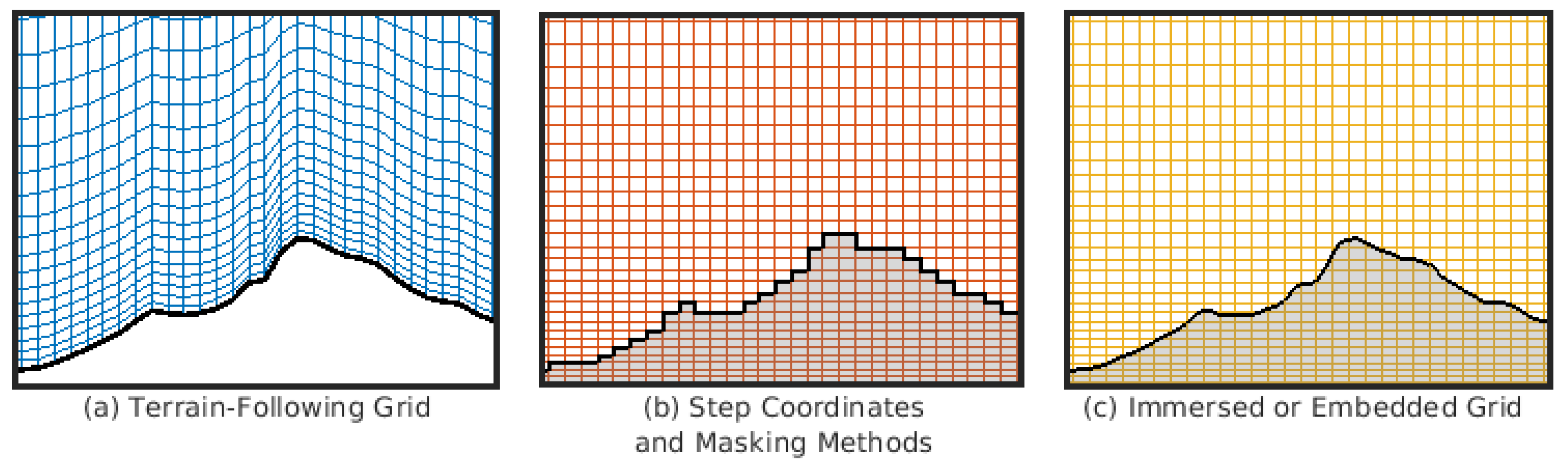
6. Representing Topography

6.1. Topographic Datasets

In the early days of numerical modeling, topographic datasets were not yet readily available, and certainly not in the digitized versions that are commonly available in a multitude of resolutions today. Rather, the first orographic maps used in atmospheric models were read out of topographic charts. For instance, Berkofsky and Bertoni [152] constructed global topographic datasets from aeronautical charts at a scale of 1:1,000,000. The topographic elevations were averaged “by eye” over one-degree squares. At the time, even the aeronautical charts were incomplete, and values “in unexplored regions were obtained by reasonable interpolations and extrapolations of known values in adjacent regions” [152]. The data were then averaged over five-degree squares and tabulated in two tables published in the article (Figure 10a). Even in the 1970s, publication of topographic datasets in the form of tables was still common in the meteorological literature. For instance, La-Valle et al. [153] published a polar stereographic map with a grid spacing of about 90 km for the European-Mediterranean region, on a grid that was intended for an early regional NWP model.

Not surprisingly, the heights of topographic obstacles were lowered dramatically by the procedures followed. For instance, in the two studies mentioned, the peak height of the Alps amounted to 1460 m and 1850 m, respectively, rather than the true peak height of 4808 m.

One of the early (then high-resolution) global datasets was ETOPO5. This is a gridded dataset of worldwide bathymetry and topography derived from several different sources at a resolution of 5 arc-minutes (about 10 km). The dataset was first published on a CD in 1988 by the US National Geophysical Data Center (NGDC). At the time of ETOPO5, better datasets did actually exist in many regions, but it was difficult to get access to such data due to traditional copyright and security restrictions imposed by most providers of topographic data.

A major jump forward came with the GLOBE dataset, the first version of which became publicly available in 1998 [154]. It provided global coverage at a spatial resolution of 30 arc-seconds (about 1 km). Later versions of this dataset benefited from the exploitation of remote sensing, such as the joint Space Shuttle Radar Topography Mapper mission in 1999, which provided complete global coverage with interferometric synthetic aperture radar (SAR) data. In 2015, NASA publicly released a refined 1 arc-second dataset (about 30 m resolution) from its Shuttle Radar Topography Mission (SRTM), which is also based on SAR [155].

6.2. Traditional Coordinate Systems and Challenges

The main challenge arising with mountains in atmospheric models is the representation of topography in the discretized numerical grid, in simulations spanning a large range of resolutions. Historically, the bottom boundary of the computational domain has been transformed to align with the terrain, referred to as “terrain-following" coordinates. This transformation has several advantages, as detailed below, but can also introduce numerical errors with steep terrain. In particular, depending upon the horizontal resolution employed, terrain-following coordinates implicitly smooth the topography, thereby significantly reduce its actual height, and thus underestimate the blocking effect of high topography. This problem was recognized already in the 1970s, and the use of “wall mountains” was proposed instead of terrain-following coordinates (for an early example, see Figure 10b). A second challenge is grid quality when spanning multiple scales. The grid aspect ratio (i.e., $\Delta x/\Delta z$) has been shown to affect simulation accuracy, and yet it is common to refine the horizontal resolution while maintaining the same vertical grid. Use of these traditional methods and challenges that arise in the gray zone are described below.

6.2.1. Pressure-Based Terrain-Following Coordinates

Traditional pressure-based coordinates are intimately tied to the use of the hydrostatic approximation. These coordinates are thus not amenable to km-scale resolutions, but serve to highlight the key challenges and solutions when representing topography in atmospheric models. In fact, two fundamental ideas were introduced with pressure coordinates, and elements of these ideas are relevant throughout all coordinate formulations available today. The first idea is the terrain-following coordinate (discussed below) and the second idea is the step coordinate system to be discussed in Section 6.3.1.

Pressure-based terrain-following coordinates were introduced by [157]. In $(x,y,p)$ space, the computational domain has an irregular lower boundary condition, as pressure surfaces intersect the ground, in particular in the presence of topography (Figure 11a). In addition, the lower boundary in p-coordinates is time-dependent, as the surface pressure $p_s=p_s(x,y,t)$ is changing in time. Terrain-following coordinates may be defined through $\sigma =\mathrm{const}$, where in the simplest case $\sigma$ is

$$\sigma :=\frac{p}{p_s}$$

(10)

This formulation yields a monotonous function from $\sigma =0$ at the model top ($p=0$) to $\sigma =1$ at the surface (see Figure 11b). With this coordinate transformation, the vertical velocity changes from $\omega =Dp/Dt$ (measured in [hPa/s]) to $\dot{\sigma }=D\sigma /Dt$ (measured in [1/s]).

The resulting implications on the governing set of equations are surprisingly mild, although the mathematical details of the coordinate transformation are complex (e.g., [158]). For instance, the horizontal momentum equation in the x-direction changes from its pressure-based version

$$\frac{Du}{Dt}-fv=-{\left(\frac{\partial \varphi }{\partial x}\right)}_p$$

(11)

to

$$\frac{Du}{Dt}-fv=-{\left(\frac{\partial \varphi }{\partial x}\right)}_{\sigma }-\frac{RT}{p_s}\frac{\partial p_s}{\partial x}$$

(12)

Here, $D/Dt$ is the total derivative (expressed in the respective coordinate system), $fv$ the Coriolis term, and $\varphi \approx gz$ the geopotential. Note that the horizontal derivatives in the pressure-gradient term are taken on p and $\sigma$-surfaces, respectively (as indicated by the subscripts).

This approach offers several advantages. First, it maps the atmospheric domain under consideration to a rectangular computational mesh whose data structure is well suited for implementation in numerical models. Second, the terrain-following coordinate transformation yields a simplification of the lower boundary condition (because the transformed vertical velocity in computational space vanishes on the bottom boundary where $\sigma =1$). Third, this alignment of the topography with $\sigma =1$ also simplifies the coupling of the dynamical core of atmospheric prediction models with boundary and surface-layer parameterization schemes.

Despite these advantages, the $\sigma$-coordinate transformation also introduces some challenges. In particular, while the pressure-gradient term is represented as one single term in the p-based system in Equation (11), two terms are required in the $\sigma$-based system in Equation (12). In cases without topography, the second term is very small. However, in regions of complex topography, both the terms are much larger than the pressure gradient itself, and this leads to potentially serious truncation errors—a problem referred to as the “pressure gradient problem”. In the horizontal direction pressure varies very slowly with the synoptic-scale pressure gradient (i.e., $\partial p/\partial x\approx 10\mathrm{hPa}/1000\mathrm{km}={10}^{-2}\mathrm{hPa}/\mathrm{km}$) while in the vertical it varies very quickly with the hydrostatic equation ($\partial p/\partial z=-gp/\left(RT\right)\approx 100\mathrm{hpa}/\mathrm{km}$). As a result, there are large cancellations between the two terms, and (relatively) small truncation errors in each of the two terms in Equation (12) may lead to serious inaccuracies in numerical estimates of the pressure gradient term. To reduce this kind of truncation error, most models introduce a hydrostatically balanced reference state, and the prognostic equations are formulated for the perturbation quantities. However, this approach does not fully eliminate the problem, as deviations from the reference state may be significant, for instance in the vicinity of strong inversions or horizontal temperature gradients. Several approaches have been proposed to further reduce these difficulties (e.g., [159,160]) but a fully satisfactory solution does not exist. Inaccuracies can also arise in the calculation of horizontal gradients for other terms, such as (implicit or explicit) horizontal diffusion (e.g., [161]).

There are several important generalizations of the $\sigma$-coordinate systems. First, most atmospheric models use an uneven spacing of the model levels, usually to enhance the representation of processes in the lower boundary. This approach also enables a cost-effective representation of the upper atmosphere in models with a high model top. Second, many models use hybrid coordinate systems. The most common system employs a transition from $\sigma$ to p-coordinates [162,163]. This improves the representation of stratospheric and mesospheric processes, where the flow is usually quasi-horizontal and where residual topographic patterns in the coordinate surface are undesired. A further generalization has been proposed by Zhu et al. [164]. They developed a formulation with smooth transitions from $\sigma$ to $\theta$ to p-coordinates, where $\theta$ denotes the potential temperature. Such a system has attractive dynamical properties in the stratosphere.

6.2.2. Height-Based Terrain-Following Coordinates

The basic form of height-based terrain-following coordinates was introduced by Gal-Chen and Somerville [165]. The idea closely follows that of the $\sigma$-coordinates, but with a z-based formulation. The coordinate surfaces are defined by $\widehat{z}=\mathrm{const}$, with

$$\widehat{z}(x,y,z):=H\frac{z-h(x,z)}{H-h(x,z)}$$

(13)

Here, H denotes the height of the model top, $h(x,y)$ the topographic height, and $\widehat{z}$ is the new vertical coordinate ranging from 0 at the surface to H at the model top.

For the transformation, the governing equations are rewritten in a vector-invariant form, which always retains their shape irrespective of the underlying coordinates. For instance, the continuity equation in z-coordinates reads

$$\frac{\partial \rho }{\partial t}+\nabla ·\left(\mathbf{u}\rho \right)=0$$

(14)

In vector-invariant notation this equation remains formally valid in any curvilinear coordinate framework. More specifically, with an alternate vertical coordinate $\widehat{z}(x,y,z)$, the transformed continuity equation can be expressed as

$$\frac{\partial \widehat{\rho }}{\partial t}+\nabla ·\left(\widehat{\mathbf{u}}\widehat{\rho }\right)=0$$

(15)

where $\widehat{\mathit{u}}=(u,v,\widehat{w})$ denotes the three-dimensional wind in transformed coordinates, with the transformed vertical velocity defined in the usual way as the total derivative

$$\widehat{w}=\frac{D\widehat{z}}{Dt}$$

(16)

and where the transformed density is

$$\widehat{\rho }=J^{-1}\rho$$

(17)

Here, $J=\frac{\partial \widehat{z}}{\partial z}$ is the Jacobian (or more precisely, the determinant of the transformation’s Jacobian). It can be seen that Equations (14) and (15) are formally identical, but the meaning of the different terms is changing. For simple equations (such as the continuity equation), the transformation is rather straightforward, but for more complicated equations (such as the viscous terms of the Navier–Stokes equation) the transformation can become very cumbersome.

Figure 12a shows the distribution of vertical coordinates in a vertical cross section using the above-discussed approach. One serious disadvantage is apparent: while at low levels the coordinates have to follow the rough underlying topography by design, there are topographic imprints on the coordinate levels even in the upper troposphere and lower stratosphere. This problem can be alleviated partially by hybrid coordinates, but not completely. As the coordinate formulation (Equation (13)) relies on a linear decay of terrain features with height, the spectrum of vertical variations in coordinate height will contain small-scale variations, even at elevated levels. It is evident that the associated grid deformations are detrimental to the quality of the numerical solution. Consider for instance a meteorological situation where the upper-level flow is quasi-horizontal and not experiencing the underlying topography (as is actually often the case). In such circumstances, it is inconvenient from a numerical perspective to use a conventional terrain-following coordinate, as a quasi-horizontal flow will—in computational space—ascend and descend through the computational mesh with the underlying topographic variations.

The difficulty under consideration can be quantified using the order-of-accuracy measure of numerical analysis. This measure is used to assess one of the most important properties of numerical algorithms—namely, how the truncation error converges to zero as the computational mesh is refined [166]. Theoretical analysis shows that the grid deformations may actually dominate the truncation error, in particular when large-scale smooth flow properties are advected across small-scale grid deformations [167]. It is thus of advantage to use terrain-following surfaces that do not exhibit a linear decay of terrain features with height (as is the case with standard terrain-following coordinates), but rather a faster (e.g., exponential) decay with height (see Figure 12b). Several versions of this idea have been proposed [163,167,168,169] and implemented in a number of limited-area and global models [167,170,171,172].

Terrain-following height coordinates are currently a preferred method in mesoscale research models, as well as numerical weather prediction and climate models. The main advantages have already been discussed in the context of $\sigma$-coordinates: a rectangular mesh in computational space, simplified implementation of lower boundary conditions, and an efficient coupling to the planetary boundary layer and soil schemes (see Figure 12). Several of these advantages are particularly appealing in lower-resolution models, where terrain-following coordinates have small slopes and are quasi horizontal. With the advent of high-resolution models, the balance of advantages and disadvantages may shift.

6.3. Alternative Gridding Techniques

As atmospheric models are used at increasingly fine resolutions, very fine-scale details of the terrain can be captured. For mountainous terrain, this means that the terrain slopes represented by the model become steeper. At very high resolutions, there is interest in capturing the effects of vertical or near-vertical features, such as those formed by cliffs, escarpments, and even the built environment. As mentioned in the previous section on terrain-following coordinates, models using those coordinate systems are challenged by numerical errors which increase in the presence of steep slopes. In an effort to develop atmospheric models that can handle arbitrarily complex terrain, alternatives to terrain-following coordinates have been developed (for more detail, see [10]). Alternative methods commonly applied when transitioning from simulating the mesoscale to microscale include wall mountains, step coordinates, masking methods, and immersed or embedded boundary methods. A section of a terrain-following grid is shown in Figure 13, along with alternative methods. This figure focuses on details of a peak of Granite Mountain in Utah, USA, whose full topography is shown in Figure 14.

6.3.1. Wall-Mountains and Step Coordinates

The second key innovation introduced with pressure coordinates mentioned above relates to the introduction of wall-mountains. The basic idea goes back to Egger [173], who argued that $\sigma$-coordinates would do well with representing large-scale lifting and ascent associated with major mountain ranges such as Greenland and Antarctica, but not with orographic blocking associated with steep mid-latitude mountain ranges such as the Alps. Indeed, a high knife-edge mountain would be smoothed to zero in $\sigma$-coordinates, when in fact it would stop all air from flowing normal to it. Egger [173] designed a wall-mountain topography, by enforcing the condition $v_n=0$, where $v_n$ is the component of the horizontal wind normal to the mountain ridge. Distinct from $\sigma$-coordinates, which approximately conserve the mountain volume (or even increase it if some form of envelope topography is used), wall mountains have zero volume but represent the blocking effect. The approach was successful and led to the first numerical simulation of Alpine lee cyclogenesis [156]. A sample of the results is shown in Figure 10b. Of course, this approach is not an option for a weather forecasting model. In particular, in real-case settings the flow response of a mountain range may involve both blocked and lifting regimes depending upon environmental conditions, while the wall-coordinate is only suitable for the former.

Mesinger et al. [174] designed a “step” mountain coordinate system (also referred to as the “eta” coordinate). In this system, the mountains are constructed from cuboid-shaped blocks with vertical walls, thereby allowing application of the $v_n=0$ condition at the lateral edges of the building blocks. This was motivated by the difficulties of the $\sigma$ system with the pressure gradient term, associated with the non-cancellation of errors in the two terms in Equation (12). With step-mountain coordinates, these difficulties do not occur, as the coordinate surfaces are quasi-horizontal. The step-mountain coordinate has served in the Eta operational model at the National Center for Environmental Prediction, but it has difficulties in representing gravity waves and produces errors along the terrain surface where artificial vorticity is introduced at step corners [175,176].

In simulations of flow over urban areas, step-coordinates can be referred to as masking methods. In these simulations, building topography is fit to the grid and boundary conditions are applied within the domain. This method is easy to implement and frequently gives good results, but introduces errors both in the approximation of the terrain and with artificial flow features appearing in step corners.

6.3.2. Immersed and Embedded Boundary Methods

As with step coordinates and masking methods, a non-conforming grid is used with immersed or embedded boundary methods, meaning that the grid is not transformed to conform to the terrain (Figure 13). Instead, the terrain passes through the fluid domain, and the effect of the terrain is represented on the flow through special treatment at the boundaries. Immersed boundaries use a “fictitious” force added to the governing equations to represent the effects of the boundary, while with embedded boundary methods the numerical discretization is modified at cells intersected by the boundary. Both methods yield a more accurate representation of the terrain than use of step coordinates and masking methods, where errors are introduced by the zeroth-order block terrain representation, as shown for example, in simulations of the Salt Lake valley using a horizontal resolution of 850 m and step coordinates [177].

Use of immersed and embedded boundaries first appeared in the engineering literature, where the methods were used to represent objects with complex geometries. Peskin [178] first used the immersed boundary method (IBM) to model two-dimensional flow through the valve of a heart, and the methods have subsequently been applied to a large variety of engineering applications [179,180]. Non-conforming gridding techniques have been employed in atmospheric applications as well, especially as higher-resolution simulations allow explicit representation of complex topographies with steep slopes. Early application of immersed or embedded boundaries to environmental applications include simulations of flow over smooth hills in ocean or atmospheric models [181,182,183]. Senocak et al. [184] used an immersed boundary to model neutral atmospheric boundary layer flow over flat terrain, focusing on correctly modeling surface stress. Simulations over the urban terrain of Baltimore, MD were carried out in Tseng et al. [185]. Lundquist et al. [9,186] implemented the immersed boundary method in the WRF model and used the method to simulate flows over urban and mountainous terrain. Flow over Bolund hill, the site of a field and model intercomparison study [187,188], has been used to validate implementations of a IBM in several different numerical models [189,190,191,192].

Although immersed and embedded boundary methods have been used successfully, several challenges remain for using non-conforming grid methods for atmospheric applications. Engineering applications frequently use high-resolution grids near objects with complex topology, employing advanced gridding techniques to achieve such high resolutions (e.g., unstructured grids, block grid refinement, and adaptive mesh refinement). This high resolution of the boundary layer allows introduction of interpolated boundary conditions with negligible error. Use of non-conforming methods can be more challenging in atmospheric applications than in engineering applications, partially because atmospheric models tend to lack flexible gridding features, but also because the high-Reynolds number flows in atmospheric applications have coarse resolution near boundaries, comparatively. This coarser resolution can introduce significant interpolation errors when alternative boundary condition treatments are used, and therefore these alternative gridding techniques are more accurate for highly resolved flows than for simulations within the gray zone. In comparison to engineering applications, additional unique challenges also arise with the parameterization of atmospheric physics. For example, parameterizations of surface fluxes are based on Monin–Obukhov similarity theory and commonly rely on use of a reference height. With terrain-following coordinates the first grid point is located at a relatively uniform height above the terrain surface, which works well with similarity theory. In contrast, non-conforming grid methods lack uniform grid spacing above the terrain, thus accurate implementation of models based on similarity theory can be difficult.

Recently, these challenges have begun to be addressed in the literature. Early implementations to combine a stress-type boundary condition with the immersed boundary method showed success in simulations of a neutral atmospheric boundary layer; however, due to use of flat topography, the stress condition was simplified to a one-dimensional implementation [184,193]. Later methods for combining IBM with a stress boundary condition extended the method to three dimensions, accommodating complex terrain. Several different implementations of IBM with a shear-stress boundary condition have been developed and validated using observations from the Askervein or Bolund hill field experiments [189,190,191,192,194]. These simulations, however, were conducted at the microscale using horizontal resolutions ranging from 1 to 5 m, rather than within the gray zone. DeLeon et al. [192] simulated flow over Askervein hill at slightly coarser horizontal resolutions, ranging from approximately 12 to 25 m. Comparisons with observations were noticeably degraded on the coarse mesh. Bao et al. [195] implemented multiple IBM methods into the WRF model and found degraded performance across implementations for flow in an idealized valley using a horizontal resolution of 90 m, indicating that development of an IBM method for the gray zone is still an open area of research.

Additional challenges beyond accurate specification of surface fluxes exist when using non-conforming grids for atmospheric simulations. One is that atmospheric physics models (e.g., radiation, land-surface, microphysics, etc.) require modification to work with alternative grids, because the bottom grid level no longer aligns with the topography. Therefore, each physics model requires modification to correctly ingest values located at the immersed boundary rather than at the lowest grid level and also to neglect portions of the computational domain which are below the terrain surface. It is also important to keep in mind that, even when atmospheric physics models are correctly coupled to the non-conforming grid, they may not work well over complex terrain or within the gray zone. Lundquist et al. [9] coupled an IBM to a subset of atmospheric physics parameterizations (e.g., radiation and land-surface) within the WRF model, providing important surface fluxes of heat and moisture for simulations of valley flows. Arthur et al. [196] extended this work by coupling a topographic shading routine to the IBM and simulated katabatic flow over Granite Mountain during the MATERHORN field campaign using horizontal resolutions of 25 and 50 m (shown in Figure 14). While surface fluxes of heat and moisture are parameterized in these works, a no-slip boundary condition for velocity was used due to the previously mentioned difficulties with accurate implementation of a surface momentum flux at immersed boundaries for simulations within the gray zone.

Further complicating the use of alternative gridding methods is that a boundary condition is required for each prognostic equation and sometimes for other model quantities, such as eddy viscosity or shear stress. For atmospheric models, this can mean setting immersed/embedded boundary conditions for dozens of variables, often with varying types of boundary conditions, leading to a more complex implementation than found in engineering applications. Additionally, although these methods are suitable for representing resolved terrain-features, smaller scale terrain frequently exists and may require special treatment. Tseng et al. [185] demonstrated that 6–8 grid points are required across a building for the immersed boundary method to produce acceptable results. Under-resolved features could be represented as virtual terrain or buildings with areas of increased drag [197].

Finally, challenges remain with obtaining realistic lateral boundary conditions for models using alternative grids, and often these simulations use idealized flow conditions at lateral boundaries instead. Wiersema et al. [35] developed a method for nesting domains using immersed boundary coordinates into those using terrain-following coordinates, and performed a multi-scale simulation of flow over urban terrain ($\Delta x$ = 2 m) nested within a mesoscale simulation ($\Delta x$ = 6 km) using a five domain configuration. The urban scale simulation ran concurrently with the mesoscale simulation, receiving time-varying lateral boundary conditions, and validation against the Joint Urban 2003 field campaign in Oklahoma City was performed. This simulation used the WRF model with its framework for concurrent nesting, along with vertical mesh refinement [53] and an immersed boundary method using a surface stress parameterization [194].

Currently, it is clear that terrain-following coordinates produce large errors when the grid becomes skewed over steep complex terrain. This is a significant challenge for producing accurate simulations within the gray zone. Several methods for handling complex terrain have been developed ranging from more accurate discretization methods, to alternative terrain-following coordinates that flatten quickly with altitude, to the alternative coordinate systems described here. Alternative coordinates, specifically immersed and embedded boundaries, have shown great promise in improving the accuracy of simulations in the gray zone over complex terrain, especially for near surface quantities such as wind speed and direction. While these methods show promise, they have primarily been employed in simulations using a dynamical core alone at microscale resolutions. Development of alternative coordinate systems for both fully featured atmospheric models and for use in the gray zone is the subject of ongoing research.

7. Discussion and Future Needs

Weather predictions at regional and fine scales increasingly play a critical role in everyday life, affecting economic, personal, and environmental decisions, among others. The atmospheric simulations used to make these predictions traverse multiple gray zones in the transition from the mesoscale to the microscale, where traditional modeling approaches may fail. In complex terrain applications, the gray zones include the representation of turbulence and convective processes and also the representation of topography, among others. Because these multiscale forecasts are the drivers not only for weather prediction but also for air quality models, regional climate simulations and wind energy applications, the impacts of improved modeling techniques in the gray zone are potentially huge.

Current mesoscale simulations have already surpassed the typical resolutions they were designed for, crossing the threshold beyond which traditional parameterization schemes may be suitable. At the same time, fine scale models are now becoming feasible over much larger regions, where mesoscale variability must naturally be incorporated, especially over complex terrain. It is clear that atmospheric simulation is a multi-scale endeavor, and one which will see tremendous opportunities in the number and type of applications as modeling techniques conquer these multiple gray zones. It is evident that for the next 10–20 years most operational and research applications of atmospheric models—in the areas of numerical weather prediction, air quality and climate modeling—will refine their spatial resolutions, but most will still not fully resolve all of the key underlying processes. In other words, they will be operating somewhere in the “gray continuum”. Experience presented in this article shows that awareness of these challenges is of key importance in advancing the accuracy and predictive power of these models.

The scale-aware formulations discussed in this review paper for grid nesting and turbulence closures from 10 km to 10 m horizontal resolutions across the gray zone or terra incognita will move models toward a consistent representation of turbulent and resolved motions as grid resolutions increase with advances in computing power. For turbulence closures, scale-aware parameterization means incorporating the grid length scale and enabling a smooth transition from PBL to LES-type closures. Moreover, the active role of unresolved turbulence in the gray zone requires new capabilities, such as representing anisotropy and backscatter, to be built into turbulence closures. The increased complexity of the resolved topography at fine scales will additionally mean that models may benefit from 3D turbulence parameterizations. For convective parameterizations, safely traversing the gray zone may mean ramping down the activity of the convection scheme toward cloud resolving simulations or using stochastic methods. Over complex terrain, the sensitivity of orographic precipitation estimates to grid resolution demonstrate the strong interplay between topography, which is increasingly resolved, and the convective representation, either of which may fall within the gray zone. Finally, underlying all of these issues is the representation of topography at different scales. While terrain-following coordinates serve well at coarse resolutions, at very fine scales, alternative gridding techniques, such as immersed boundary methods, enable simulations of very steep topography. The transition across these scales will no doubt bring innovation in new hybrid coordinate systems that perhaps combine the best parts of both terrain-following and IBM approaches in the gray zone.

Future research efforts in all of these areas must be devoted to continue to ensure that mesoscale models are using cutting edge physics parameterizations and numerical methods. Well-organized intercomparison projects will help the community to expedite the progress and identify the best modeling strategies to provide physically consistent simulations across a wide range of scales over complex terrain.

References

1. De Wekker, S.F.J.; Kossmann, M.; Knievel, J.C.; Giovannini, L.; Gutmann, E.D.; Zardi, D. Meteorological Applications Benefiting from an Improved Understanding of Atmospheric Exchange Processes over Mountains. Atmosphere 2018, 9, 371. [Google Scholar] [CrossRef]
2. Zardi, D.; Whiteman, C. Diurnal mountain wind systems. In Mountain Weather Research and Forecasting; Chow, F., Wekker, S.D., Snyder, B., Eds.; Springer: Berlin, Germany, 2013; pp. 35–119. [Google Scholar]
3. Jackson, P.; Mayr, G.; Vosper, S. Dynamically-driven winds. In Mountain Weather Research and Forecasting; Chow, F., Wekker, S.D., Snyder, B., Eds.; Springer: Berlin, Germany, 2013; pp. 121–218. [Google Scholar]
4. Lehner, M.; Rotach, M.W. Current Challenges in Understanding and Predicting Transport and Exchange in the Atmosphere over Mountainous Terrain. Atmosphere 2018, 9, 276. [Google Scholar] [CrossRef]
5. Efstathiou, G.A.; Beare, R.J.; Osborne, S.; Lock, A.P. Grey zone simulations of the morning convective boundary layer development. J. Geophys. Res. Atmos. 2016, 121, 4769–4782. [Google Scholar] [CrossRef] [Green Version]
6. Wyngaard, J.C. Toward numerical modeling in the “Terra Incognita”. J. Atmos. Sci. 2004, 61, 1816–1826. [Google Scholar] [CrossRef]
7. Chow, F.K.; Weigel, A.P.; Street, R.L.; Rotach, M.W.; Xue, M. High-resolution large-eddy simulations of flow in a steep Alpine valley. Part I: Methodology, verification, and sensitivity studies. J. Appl. Meteorol. Climatol. 2006, 45, 63–86. [Google Scholar] [CrossRef]
8. Mirocha, J.D.; Kosovic, B.; Aitken, M.L.; Lundquist, J.K. Implementation of a generalized actuator disk wind turbine model into the weather research and forecasting model for large-eddy simulation applications. J. Renew. Sustain. Energy 2014, 6. [Google Scholar] [CrossRef]
9. Lundquist, K.A.; Chow, F.K.; Lundquist, J.K. An Immersed Boundary Method for the Weather Research and Forecasting Model. Mon. Weather Rev. 2010, 138, 796–817. [Google Scholar] [CrossRef]
10. Lundquist, K.; Chow, F. Flow over complex terrain, numerical modeling of. In Encyclopedia of Environmetrics; El-Shaarawi, A., Piegorsch, W., Eds.; John Wiley and Sons, Ltd.: Hoboken, NJ, USA, 2012; pp. 1054–1063. [Google Scholar] [CrossRef]
11. Ban, N.; Schmidli, J.; Schär, C. Evaluation of the convection-resolving regional climate modeling approach in decade-long simulations. JGR Atmos. 2014, 119, 7889–7907. [Google Scholar] [CrossRef] [Green Version]
12. Panosetti, D.; Böing, S.; Schlemmer, L.; Schmidli, J. Idealized Large-Eddy and Convection-Resolving Simulations of Moist Convection over Mountainous Terrain. J. Atmos. Sci. 2016, 73, 4021–4041. [Google Scholar] [CrossRef]
13. Zhou, B.; Simon, J.S.; Chow, F.K. The Convective Boundary Layer in the Terra Incognita. J. Atmos. Sci. 2014, 71, 2545–2563. [Google Scholar] [CrossRef]
14. Richard, E.; Buzzi, A.; Zängl, G. Quantitative precipitation forecasting in the Alps: The advances achieved by the Mesoscale Alpine Programme. Q. J. R. Meteorol. Soc. 2007, 133, 831–846. [Google Scholar] [CrossRef] [Green Version]
15. Bryan, G.; Wyngaard, J.; Fritsch, J. Resolution requirements for the simulation of deep moist convection. Mon. Weather Rev. 2003, 131, 2394–2416. [Google Scholar] [CrossRef]
16. Fuhrer, O.; Osuna, C.; Lapillonne, X.; Gysi, T.; Cumming, B.; Bianco, M.; Arteaga, A.; Schulthess, T.C. Towards a per- formance portable, architecture agnostic implementation strategy for weather and climate models. Supercomput. Front. Innov. 2014, 1, 44–61. [Google Scholar] [CrossRef]
17. Schalkwijk, J.; Jonker, H.J.J.; Siebesma, A.P.; Bosveld, F.C. A year-long large-eddy simulation of the weather over Cabauw: An overview. Mon. Weather Rev. 2015, 143, 828–844. [Google Scholar] [CrossRef]
18. Fuhrer, O.; Chadha, T.; Hoefler, T.; Kwasniewski, G.; Lapillonne, X.; Leutwyler, D.; Lüthi, D.; Osuna, C.; Schär, C.; Schulthess, T.C.; et al. Near-global climate simulation at 1 km resolution: establishing a performance baseline on 4888 GPUs with COSMO 5.0. Geosci. Model Dev. 2018, 11, 1665–1681. [Google Scholar] [CrossRef]
19. Leutwyler, D.; Lüthi, D.; Ban, N.; Fuhrer, O.; Schär, C. Evaluation of the Convection-Resolving Climate Modeling Approach on Continental Scales. J. Geophys. Res.-Atmos. 2017. [Google Scholar] [CrossRef]
20. Schulthess, T.; Bauer, P.; Fuhrer, O.; Hoefler, T.; Schär, C.; Wedi, N. Reflecting on the goal and baseline for Exascale Computing: A roadmap based on weather and climate simulations. IEEE Comput. Sci. Eng. 2019, 21, 30–41. [Google Scholar] [CrossRef]
21. Vosper, S.B.; Ross, A.N.; Renfrew, I.A.; Sheridan, P.; Elvidge, A.D.; Grubišić, V. Current Challenges in Orographic Flow Dynamics: Turbulent Exchange Due to Low-Level Gravity-Wave Processes. Atmosphere 2018, 9, 361. [Google Scholar] [CrossRef]
22. Zhou, B.; Chow, F.K. Nested Large-Eddy Simulations of the Intermittently Turbulent Stable Atmospheric Boundary Layer over Real Terrain. J. Atmos. Sci. 2014, 71, 1021–1039. [Google Scholar] [CrossRef]
23. Zhong, S.; Chow, F.K. Meso-and fine-scale modeling over complex terrain: Parameterizations and applications. In Mountain Weather Research and Forecasting; Chow, F., Wekker, S.D., Snyder, B., Eds.; Springer: Berlin, Germany, 2013; pp. 591–653. [Google Scholar]
24. Goger, B.; Rotach, M.W.; Gohm, A.; Fuhrer, O.; Stiperski, I.; Holtslag, A.A. The Impact of Three-Dimensional Effects on the Simulation of Turbulence Kinetic Energy in a Major Alpine Valley. Bound.-Layer Meteorol. 2018, 168, 1–27. [Google Scholar] [CrossRef] [PubMed] [Green Version]
25. Leung, L.; Kuo, Y.; Tribbia, J. Research needs and directions of regional climate modeling using WRF and CCSM. Bull. Am. Meteorl. Soc. 2006, 87, 1747–1751. [Google Scholar] [CrossRef]
26. Hohenegger, C.; Brockhaus, P.; Schar, C. Towards climate simulations at cloud-resolving scales. Meteorol. Z. 2008, 17, 383–394. [Google Scholar] [CrossRef]
27. Knote, C.; Heinemann, G.; Rockel, B. Changes in weather extremes: Assessment of return values using high resolution climate simulations at convection-resolving scale. Meteorol. Z. 2010, 19, 11–23. [Google Scholar] [CrossRef]
28. Giovannini, L.; Zardi, D.; de Franceschi, M.; Chen, F. Numerical simulations of boundary-layer processes and urban-induced alterations in an Alpine valley. Int. J. Climatol. 2014, 34, 1111–1131. [Google Scholar] [CrossRef]
29. Kendon, E.J.; Roberts, N.M.; Fowler, H.J.; Roberts, M.J.; Chan, S.C.; Senior, C.A. Heavier summer downpours with climate change revealed by weather forecast resolution model. Nat. Clim. Chang. 2014, 4, 570–576. [Google Scholar] [CrossRef]
30. Arakawa, A.; Jung, J.H.; Wu, C.M. Toward unification of the multiscale modeling of the atmosphere. Atmos. Chem. Phys. 2011, 11, 3731–3742. [Google Scholar] [CrossRef] [Green Version]
31. Skamarock, W.C.; Klemp, J.B.; Duda, M.G.; Fowler, L.D.; Park, S.H.; Ringler, T.D. A Multiscale Nonhydrostatic Atmospheric Model Using Centroidal Voronoi Tesselations and C-Grid Staggering. Mon. Weather Rev. 2012, 140, 3090–3105. [Google Scholar] [CrossRef] [Green Version]
32. Mearns, L.; Bogardi, I.; Giorgi, F.; Matyasovszky, I.; Palecki, M. Comparison of climate change scenarios generated from regional climate model experiments and statistical downscaling. J. Geophys. Res.-Atmos. 1999, 104, 6603–6621. [Google Scholar] [CrossRef] [Green Version]
33. Leung, L.; Mearns, L.; Giorgi, F.; Wilby, R. Regional climate research—Needs and opportunities. Bull. Am. Meteorol. Soc. 2003, 84, 89–95. [Google Scholar]
34. Munoz-Esparza, D.; Lundquist, J.K.; Sauer, J.A.; Kosovic, B.; Linn, R.R. Coupled mesoscale-LES modeling of a diurnal cycle during the CWEX-13 field campaign: From weather to boundary-layer eddies. J. Adv. Model. Earth Syst. 2017, 9, 1572–1594. [Google Scholar] [CrossRef] [Green Version]
35. Wiersema, D.; Lundquist, K.; Chow, F. Development of a Multi-Scale Modeling Framework for Urban Simulations in the Weather Research and Forecasting Model. In Proceedings of the 23rd Symposium on Boundary Layers and Turbulence, Oklahoma City, OK, USA, 11–15 June 2018; American Meteorological Society: Boston, MA, USA, 2018. [Google Scholar]
36. Moeng, C.; Dudhia, J.; Klemp, J.; Sullivan, P. Examining two-way grid nesting for large eddy simulation of the PBL using the WRF model. Mon. Weather Rev. 2007, 135, 2295–2311. [Google Scholar] [CrossRef]
37. Marjanovic, N.; Wharton, S.; Chow, F. Investigation of model parameters for high-resolution wind energy forecasting: case studies over simple and complex terrain. J. Wind Eng. Ind. Aerodyn. 2018, 134, 10–24. [Google Scholar] [CrossRef]
38. Davies, H. Limitations of some common lateral boundary schemes used in regional NWP models. Mon. Weather Rev. 1983, 111, 1002–1012. [Google Scholar] [CrossRef]
39. Warner, T.T.; Peterson, R.A.; Treadon, R.E. A tutorial on lateral boundary conditions as a basic and potentially serious limitation to regional numerical weather prediction. Bull. Am. Meteorol. Soc. 1997, 78, 2599–2618. [Google Scholar] [CrossRef]
40. Simon, J.; Zhou, B.; Mirocha, J.; Chow, F. Explicit filtering and reconstruction to reduce grid dependence in convective boundary layer simulations using WRF-LES. Mon. Weather Rev. 2019, in press. [Google Scholar] [CrossRef]
41. Langhans, W.; Schmidli, J.; Schär, C. Bulk convergence of cloud-resolving simulations of moist convection over complex terrain. J. Atmos. Sci. 2012, 69, 2207–2228. [Google Scholar] [CrossRef]
42. Kelly, R. The onset and development of thermal convection in fully developed shear flows. Adv. Appl. Mech. 1994, 31, 35–112. [Google Scholar] [CrossRef]
43. Munoz-Esparza, D.; Kosovic, B.; van Beeck, J.; Mirocha, J. A stochastic perturbation method to generate inflow turbulence in large-eddy simulation models: Application to neutrally stratified atmospheric boundary layers (vol 27, 035102, 2015). Phys. Fluids 2015, 27. [Google Scholar] [CrossRef]
44. Kirkil, G.; Mirocha, J.; Bou-Zeid, E.; Chow, F.K.; Kosović, B. Implementation and Evaluation of Dynamic Subfilter-Scale Stress Models for Large-Eddy Simulation Using WRF. Mon. Weather Rev. 2012, 140, 266–284. [Google Scholar] [CrossRef]
45. Houze, R.A. Cloud Dynamics; International Geophysics Series; Academic Press: San Diego, CA, USA, 2003; Volume 53, 570p. [Google Scholar]
46. Brisson, E.; Demuzere, M.; van Lipzig, N.P. Modelling strategies for performing convection-permitting climate simulations. Meteorol. Z. 2016, 25, 149–163. [Google Scholar] [CrossRef]
47. Mirocha, J.; Kirkil, G.; Bou-Zeid, E.; Chow, F.K.; Kosović, B. Transition and Equilibration of Neutral Atmospheric Boundary Layer Flow in One-Way Nested Large-Eddy Simulations Using the Weather Research and Forecasting Model. Mon. Weather Rev. 2012, 141, 918–940. [Google Scholar] [CrossRef]
48. Goodfriend, E.; Chow, F.K.; Vanella, M.; Balaras, E. Improving Large-Eddy Simulation of Neutral Boundary Layer Flow across Grid Interfaces. Mon. Weather Rev. 2015, 143, 3310–3326. [Google Scholar] [CrossRef]
49. Mirocha, J.; Kosović, B.; Kirkil, G. Resolved Turbulence Characteristics in Large-Eddy Simulations Nested within Mesoscale Simulations Using the Weather Research and Forecasting Model. Mon. Weather Rev. 2014, 142, 806–831. [Google Scholar] [CrossRef]
50. Munoz-Esparza, D.; Kosovic, B. Generation of Inflow Turbulence in Large-Eddy Simulations of Nonneutral Atmospheric Boundary Layers with the Cell Perturbation Method. Mon. Weather Rev. 2018, 146, 1889–1909. [Google Scholar] [CrossRef]
51. Mazzaro, L.J.; Munoz-Esparza, D.; Lundquist, J.K.; Linn, R.R. Nested mesoscale-to-LES modeling of the atmospheric boundary layer in the presence of under-resolved convective structures. J. Adv. Model. Earth Syst. 2017, 9, 1795–1810. [Google Scholar] [CrossRef] [Green Version]
52. Van Veen, L. The Perdigão Field Campaign: Evaluation of the Cell Perturbation Method in Atmospheric Simulations. Master’s Thesis, University of Twente, Enschede, The Netherlands, 2018. [Google Scholar]
53. Daniels, M.H.; Lundquist, K.A.; Mirocha, J.D.; Wiersema, D.J.; Chow, F.K. A New Vertical Grid Nesting Capability in the Weather Research and Forecasting (WRF) Model. Mon. Weather Rev. 2016, 144, 3725–3747. [Google Scholar] [CrossRef]
54. Mirocha, J.D.; Lundquist, K.A. Assessment of Vertical Mesh Refinement in Concurrently Nested Large-Eddy Simulations Using the Weather Research and Forecasting Model. Mon. Weather Rev. 2017, 145, 3025–3048. [Google Scholar] [CrossRef]
55. Ching, J.; Rotunno, R.; LeMone, M.; Martilli, A.; Kosovic, B.; Jimenez, P.; Dudhia, J. Convectively induced secondary circulations in fine-grid mesoscale numerical weather prediction models. Mon. Weather Rev. 2014, 142, 3284–3302. [Google Scholar] [CrossRef]
56. Yano, J.I.; Ziemiański, M.Z.; Cullen, M.; Termonia, P.; Onvlee, J.; Bengtsson, L.; Carrassi, A.; Davy, R.; Deluca, A.; Gray, S.L.; et al. Scientific Challenges of Convective-Scale Numerical Weather Prediction. Bull. Am. Meteorol. Soc. 2018, 99, 699–710. [Google Scholar] [CrossRef] [Green Version]
57. Shi, X.; Chow, F.K.; Street, R.L.; Bryan, G.H. An Evaluation of LES Turbulence Models for Scalar Mixing in the Stratocumulus-Capped Boundary Layer. J. Atmos. Sci. 2018, 75, 1499–1507. [Google Scholar] [CrossRef]
58. Deardorff, J.W. Stratocumulus-capped mixed layers derived from a three-dimensional model. Bound.-Layer Meteorol. 1980, 18, 495–527. [Google Scholar] [CrossRef]
59. Verrelle, A.; Ricard, D.; Lac, C. Evaluation and Improvement of Turbulence Parameterization inside Deep Convective Clouds at Kilometer-Scale Resolution. Mon. Weather Rev. 2017, 145, 3947–3967. [Google Scholar] [CrossRef]
60. Shi, X.; Hagen, H.L.; Chow, F.K.; Bryan, G.H.; Street, R.L. Large-eddy simulation of the stratocumulus-capped boundary layer with explicit filtering and reconstruction turbulence modeling. J. Atmos. Sci. 2018, 75, 611–637. [Google Scholar] [CrossRef]
61. Bryan, G.H. Effects of surface exchange coefficients and turbulence length scales on the intensity and structure of numerically simulated hurricanes. Mon. Weather Rev. 2012, 140, 1125–1143. [Google Scholar] [CrossRef]
62. Green, B.W.; Zhang, F. Numerical simulations of Hurricane Katrina (2005) in the turbulent gray zone. J. Adv. Model. Earth Syst. 2015, 7, 142–161. [Google Scholar] [CrossRef] [Green Version]
63. Kitamura, Y. Estimating dependence of the turbulent length scales on model resolution based on a priori analysis. J. Atmos. Sci. 2015, 72, 750–762. [Google Scholar] [CrossRef]
64. Deardorff, J. The counter-gradient heat flux in the lower atmosphere and in the laboratory. J. Atmos. Sci. 1966, 23, 503–506. [Google Scholar] [CrossRef]
65. Klemp, J.B. Damping Characteristics of Horizontal Laplacian Diffusion Filters. Mon. Weather Rev. 2017, 145, 4365–4379. [Google Scholar] [CrossRef]
66. Zhou, B.; Zhu, K.; Xue, M. A Physically Based Horizontal Subgrid-Scale Turbulent Mixing Parameterization for the Convective Boundary Layer. J. Atmos. Sci. 2017, 74, 2657–2674. [Google Scholar] [CrossRef]
67. Tompkins, A.M.; Semie, A.G. Organization of tropical convection in low vertical wind shears: Role of updraft entrainment. J. Adv. Model. Earth Syst 2017, 9, 1046–1068. [Google Scholar] [CrossRef]
68. Bryan, G.H.; Rotunno, R. The maximum intensity of tropical cyclones in axisymmetric numerical model simulations. Mon. Weather Rev. 2009, 137, 1770–1789. [Google Scholar] [CrossRef]
69. Bhattacharya, R.; Stevens, B. A two Turbulence Kinetic Energy model as a scale-adaptive approach to modeling the planetary boundary layer. J. Adv. Model. Earth Syst 2016, 8, 224–243. [Google Scholar] [CrossRef]
70. Hanley, K.E.; Plant, R.S.; Stein, T.H.M.; Hogan, R.J.; Nicol, J.C.; Lean, H.W.; Halliwell, C.; Clark, P.A. Mixing-length controls on high-resolution simulations of convective storms. Q. J. R. Meteorol. Soc. 2015, 141, 272–284. [Google Scholar] [CrossRef]
71. Bryan, G.H.; Morrison, H. Sensitivity of a simulated squall line to horizontal resolution and parameterization of microphysics. Mon. Weather Rev. 2012, 140, 202–225. [Google Scholar] [CrossRef]
72. Verrelle, A.; Ricard, D.; Lac, C. Sensitivity of high-resolution idealized simulations of thunderstorms to horizontal resolution and turbulence parametrization. Q. J. R. Meteorol. Soc. 2015, 141, 433–448. [Google Scholar] [CrossRef]
73. Kurowski, M.J.; Teixeira, J. A scale-adaptive turbulent kinetic energy closure for the dry convective boundary layer. J. Atmos. Sci. 2018, 75, 675–690. [Google Scholar] [CrossRef]
74. Kitamura, Y. Improving a turbulence scheme for the Terra Incognita in a dry convective boundary layer. J. Meteorol. Soc. Jpn. Ser. II 2016, 94, 491–506. [Google Scholar] [CrossRef]
75. Hatlee, S.C.; Wyngaard, J.C. Improved subfilter-scale models from the HATS field data. J. Atmos. Sci. 2007, 64, 1694–1705. [Google Scholar] [CrossRef]
76. Ramachandran, S.; Wyngaard, J.C. Subfilter-scale modelling using transport equations: Large-eddy simulation of the moderately convective atmospheric boundary layer. Bound.-Layer Meteorol. 2011, 139, 1–35. [Google Scholar] [CrossRef]
77. Rodi, W. A new algebraic relation for calculating the Reynolds stresses. Gesellschaft Angewandte Mathematik Mechanik Workshop Paris France 1976, 56, 219–221. [Google Scholar]
78. Findikakis, A.N.; Street, R.L. An algebraic model for subgrid-scale turbulence in stratified flows. J. Atmos. Sci. 1979, 36, 1934–1949. [Google Scholar] [CrossRef]
79. Enriquez, R.M. Subgrid-Scale Turbulence Modeling for Improved Large-Eddy Simulation of the Atmospheric Boundary Layer. Ph.D. Thesis, Stanford University, Stanford, CA, USA, 2013. [Google Scholar]
80. Shi, X.; Enriquez, R.; Street, R.; Chow, F.; Bryan, G. Evaluation of an Algebraic Turbulence Closure Scheme for the Simulations of Dry and Moist Atmospheric Boundary Layers. In Proceedings of the 23rd Symposium on Boundary Layers and Turbulence, Oklahoma City, OK, USA, 11–15 June 2018; American Meteorological Society: Boston, MA, USA, 2018. [Google Scholar]
81. Shi, X.; Enriquez, R.; Street, R.; Bryan, G.; Chow, F. An Implicit Algebraic Turbulence Closure Scheme for Atmospheric Boundary Layer Simulation. J. Atmos. Sci. 2019. Submitted. [Google Scholar]
82. Chow, F.K.; Street, R.L.; Xue, M.; Ferziger, J.H. Explicit filtering and reconstruction turbulence modeling for large-eddy simulation of neutral boundary layer flow. J. Atmos. Sci. 2005, 62, 2058–2077. [Google Scholar] [CrossRef]
83. Shi, X.; Chow, F.K.; Street, R.L.; Bryan, G.H. Evaluation of Some LES-type Turbulence Parameterizations for Simulating Deep Convection at Kilometer-Scale Resolution. J. Adv. Model. Earth Syst 2018. Submitted. [Google Scholar]
84. Wong, V.C.; Lilly, D.K. A comparison of two dynamic subgrid closure methods for turbulent thermal convection. Phys. Fluids 1994, 6, 1016–1023. [Google Scholar] [CrossRef]
85. Chow, F.K.; Street, R.L. Evaluation of turbulence closure models for large-eddy simulation over complex terrain: flow over Askervein Hill. J. Appl. Meteorol. Climatol. 2009, 48, 1050–1065. [Google Scholar] [CrossRef]
86. Moeng, C.H.; Sullivan, P.; Khairoutdinov, M.; Randall, D. A mixed scheme for subgrid-scale fluxes in cloud-resolving models. J. Atmos. Sci. 2010, 67, 3692–3705. [Google Scholar] [CrossRef]
87. Ito, J.; Niino, H.; Nakanishi, M.; Moeng, C.H. An extension of the Mellor–Yamada model to the terra incognita zone for dry convective mixed layers in the free convection regime. Bound.-Layer Meteorol. 2015, 157, 23–43. [Google Scholar] [CrossRef]
88. Mellor, G.L.; Yamada, T. Development of a turbulence closure model for geophysical fluid problems. Rev. Geophys. 1982, 20, 851–875. [Google Scholar] [CrossRef]
89. Shin, H.H.; Hong, S.Y. Representation of the subgrid-scale turbulent transport in convective boundary layers at gray-zone resolutions. Mon. Weather Rev. 2015, 143, 250–271. [Google Scholar] [CrossRef]
90. Boutle, I.; Eyre, J.; Lock, A. Seamless stratocumulus simulation across the turbulent gray zone. Mon. Weather Rev. 2014, 142, 1655–1668. [Google Scholar] [CrossRef]
91. Siebesma, A.; Teixeira, J. An advection-diffusion scheme for the convective boundary layer: Description and 1D results. In Proceedings of the 14th Symposium on Boundary Layers and Turbulence, Aspen, CO, USA, 7–11 August 2000; American Meteorological Society: Boston, MA, USA, 2000; pp. 133–136. [Google Scholar]
92. Siebesma, A.P.; Soares, P.M.; Teixeira, J. A combined eddy-diffusivity mass-flux approach for the convective boundary layer. J. Atmos. Sci. 2007, 64, 1230–1248. [Google Scholar] [CrossRef]
93. Arakawa, A.; Schubert, W.H. Interaction of a cumulus cloud ensemble with the large-scale environment, Part I. J. Atmos. Sci. 1974, 31, 674–701. [Google Scholar] [CrossRef]
94. Honnert, R.; Couvreux, F.; Masson, V.; Lancz, D. Sampling the structure of convective turbulence and implications for grey-zone parametrizations. Bound.-Layer Meteorol. 2016, 160, 133–156. [Google Scholar] [CrossRef]
95. Neggers, R.A.J. Exploring bin-macrophysics models for moist convective transport and clouds. J. Adv. Model. Earth Syst 2015, 7, 2079–2104. [Google Scholar] [CrossRef] [Green Version]
96. Tan, Z.; Kaul, C.M.; Pressel, K.G.; Cohen, Y.; Schneider, T.; Teixeira, J. An Extended Eddy-Diffusivity Mass-Flux Scheme for Unified Representation of Subgrid-Scale Turbulence and Convection. J. Adv. Model. Earth Syst 2018. [Google Scholar] [CrossRef] [PubMed]
97. Larson, V.E.; Golaz, J.C. Using probability density functions to derive consistent closure relationships among higher-order moments. Mon. Weather Rev. 2005, 133, 1023–1042. [Google Scholar] [CrossRef]
98. Bogenschutz, P.A.; Krueger, S.K. A simplified PDF parameterization of subgrid-scale clouds and turbulence for cloud-resolving models. J. Adv. Model. Earth Syst 2013, 5, 195–211. [Google Scholar] [CrossRef] [Green Version]
99. Larson, V.E.; Schanen, D.P.; Wang, M.; Ovchinnikov, M.; Ghan, S. PDF parameterization of boundary layer clouds in models with horizontal grid spacings from 2 to 16 km. Mon. Weather Rev. 2012, 140, 285–306. [Google Scholar] [CrossRef]
100. Dorrestijn, J.; Crommelin, D.T.; Siebesma, A.P.; Jonker, H.J. Stochastic parameterization of shallow cumulus convection estimated from high-resolution model data. Theor. Comput. Fluid Dyn. 2013, 27, 133–148. [Google Scholar] [CrossRef]
101. Sakradzija, M.; Seifert, A.; Dipankar, A. A stochastic scale-aware parameterization of shallow cumulus convection across the convective gray zone. J. Adv. Model. Earth Syst 2016, 8, 786–812. [Google Scholar] [CrossRef] [Green Version]
102. Fiori, E.; Parodi, A.; Siccardi, F. Turbulence closure parameterization and grid spacing effects in simulated supercell storms. J. Atmos. Sci. 2010, 67, 3870–3890. [Google Scholar] [CrossRef]
103. Parodi, A.; Tanelli, S. Influence of turbulence parameterizations on high-resolution numerical modeling of tropical convection observed during the TC4 field campaign. J. Geophys. Res. Atmos. 2010, 115. [Google Scholar] [CrossRef] [Green Version]
104. Machado, L.A.; Chaboureau, J.P. Effect of turbulence parameterization on assessment of cloud organization. Mon. Weather Rev. 2015, 143, 3246–3262. [Google Scholar] [CrossRef]
105. Kirshbaum, D.J.; Adler, B.; Kalthoff, N.; Barthlott, C.; Serafin, S. Moist Orographic Convection: Physical Mechanisms and Links to Surface-Exchange Processes. Atmosphere 2018, 9, 80. [Google Scholar] [CrossRef]
106. Guichard, F.; Couvreux, F. A short review of numerical cloud-resolving models. Tellus A Dyn. Meteorol. Oceanogr. 2017, 69, 1373578. [Google Scholar] [CrossRef] [Green Version]
107. Lugauer, M.; Winkler, P. Alpines Pumpen – thermische Zirkulation zwischen Alpen und Bayrischem Alpenvorland; Arbeitsergebnisse Nr. 72; Deutscher Wetterdienst: Offenbach, Germany, 2002. [Google Scholar]
108. Weissmann, M.; Braun, F.; Gantner, L.; Mayr, G.; Rahm, S.; Reitebuch, O. The Alpine Mountain-Plain Circulation: Airborne Doppler Lidar Measurements and Numerical Simulations. Mon. Weather Rev. 2005, 133, 3095–3109. [Google Scholar] [CrossRef]
109. Mass, C. Topographically Forced Convergence in Western Washington State. Mon. Weather Rev. 1981, 109, 1335–1347. [Google Scholar] [CrossRef] [Green Version]
110. Fuhrer, O.; Schär, C. Dynamics of Orographically Triggered Banded Convection in Sheared Moist Orographic Flows. J. Atmos. Sci. 2007, 64, 3542–3561. [Google Scholar] [CrossRef]
111. Barrett, A.I.; Gray, S.L.; Kirshbaum, D.J.; Roberts, N.M.; Schultz, D.M.; Fairman, J.G. Synoptic versus orographic control on stationary convective banding. Q. J. R. Meteorol. Soc. 2014, 141, 1101–1113. [Google Scholar] [CrossRef] [Green Version]
112. Tiedtke, M. A comprehensive mass flux scheme for cumulus parameterization in large-scale models. Mon. Weather Rev. 1989, 117, 1779–1800. [Google Scholar] [CrossRef]
113. Suhas, E.; Zhang, G.J. Evaluation of Trigger Functions for Convective Parameterization Schemes Using Observations. J. Clim. 2014, 27, 7647–7666. [Google Scholar] [CrossRef]
114. Jakob, C. Accelerating Progress in Global Atmospheric Model Development through Improved Parameterizations. Bull. Am. Meteorol. Soc. 2010, 91, 869–876. [Google Scholar] [CrossRef] [Green Version]
115. Frei, C.; Christensen, J.H.; Déqué, M.; Jacob, D.; Jones, R.G.; Vidale, P.L. Daily precipitation statistics in regional climate models: Evaluation and intercomparison for the European Alps. J. Geophys. Res. Atmos. 2003, 108. [Google Scholar] [CrossRef] [Green Version]
116. Kyselý, J.; Rulfová, Z.; Farda, A.; Hanel, M. Convective and stratiform precipitation characteristics in an ensemble of regional climate model simulations. Clim. Dyn. 2016, 46, 227–243. [Google Scholar] [CrossRef]
117. Tselioudis, G.; Douvis, C.; Zerefos, C. Does dynamical downscaling introduce novel information in climate model simulations of precipitation change over a complex topography region? Int. J. Climatol. 2012, 32, 1572–1578. [Google Scholar] [CrossRef]
118. Langhans, W.; Schmidli, J.; Fuhrer, O.; Bieri, S.; Schär, C. Long-Term Simulations of Thermally Driven Flows and Orographic Convection at Convection-Parameterizing and Cloud-Resolving Resolutions. J. Appl. Meteorol. Climatol. 2013, 52, 1490–1510. [Google Scholar] [CrossRef]
119. Schwitalla, T.; Bauer, H.S.; Wulfmeyer, V.; Zängl, G. Systematic errors of QPF in low-mountain regions as revealed by MM5 simulations. Meteorol. Z. 2008, 17, 903–919. [Google Scholar] [CrossRef]
120. Pritchard, M.S.; Moncrieff, M.W.; Somerville, R.C. Orogenic Propagating Precipitation Systems over the United States in a Global Climate Model with Embedded Explicit Convection. J. Atmos. Sci. 2011, 68, 1821–1840. [Google Scholar] [CrossRef]
121. Plant, R.; Craig, G. A Stochastic Parameterization for Deep Convection Based on Equilibrium Statistics. J. Atmos. Sci. 2008, 65, 87–105. [Google Scholar] [CrossRef] [Green Version]
122. Sakradzija, M.; Seifert, A.; Heus, T. Fluctuations in a quasi-stationary shallow cumulus cloud ensemble. Nonlinear Process. Geophys. 2015, 22, 65–85. [Google Scholar] [CrossRef] [Green Version]
123. Bengtsson, L.; Steinheimer, M.; Bechtold, P.; Geleyn, J. A stochastic parametrization for deep convection using cellular automata. Q. J. R. Meteorol. Soc. 2013, 139, 1533–1543. [Google Scholar] [CrossRef] [Green Version]
124. Berner, J.; Achatz, U.; Batté, L.; Bengtsson, L.; Cámara, A.D.L.; Christensen, H.M.; Colangeli, M.; Coleman, D.R.; Crommelin, D.; Dolaptchiev, S.I.; et al. Stochastic Parameterization: Toward a New View of Weather and Climate Models. Bull. Am. Meteorol. Soc. 2016, 98, 565–588. [Google Scholar] [CrossRef]
125. Serafin, S.; Adler, B.; Cuxart, J.; De Wekker, S.F.J.; Gohm, A.; Grisogono, B.; Kalthoff, N.; Kirshbaum, D.J.; Rotach, M.W.; Schmidli, J.; et al. Exchange Processes in the Atmospheric Boundary Layer Over Mountainous Terrain. Atmosphere 2018, 9, 102. [Google Scholar] [CrossRef]
126. Grell, G.A.; Freitas, S.R. A scale and aerosol aware stochastic convective parameterization for weather and air quality modeling. Atmos. Chem. Phys. 2014, 14, 5233–5250. [Google Scholar] [CrossRef] [Green Version]
127. Kwon, Y.C.; Hong, S. A Mass-Flux Cumulus Parameterization Scheme across Gray-Zone Resolutions. Mon. Weather Rev. 2016, 145, 583–598. [Google Scholar] [CrossRef]
128. Ban, N.; Schmidli, J.; Schär, C. Heavy precipitation in a changing climate: Does short-term precipitation increase faster? Geophys. Res. Lett. 2015, 42, 1165–1172. [Google Scholar] [CrossRef]
129. Prein, A.F.; Langhans, W.; Fosser, G.; Ferrone, A.; Ban, N.; Goergen, K.; Keller, M.; Tölle, M.; Gutjahr, O.; Feser, F.; et al. A review on regional convection-permitting climate modeling: Demonstrations, prospects, and challenges. Rev. Geophys. 2015, 53, 323–361. [Google Scholar] [CrossRef]
130. Liu, C.; Ikeda, K.; Rasmussen, R.; Barlage, M.; Newman, A.J.; Prein, A.F.; Chen, F.; Chen, L.; Clark, M.; Dai, A.; et al. Continental-scale convection-permitting modeling of the current and future climate of North America. Clim. Dyn. 2017, 49, 71–95. [Google Scholar] [CrossRef]
131. Nasuno, T.; Yamada, H.; Nakano, M.; Kubota, H.; Sawada, M.; Yoshida, R. Global cloud-permitting simulations of Typhoon Fengshen (2008). Geosci. Lett. 2016, 3, 32. [Google Scholar] [CrossRef]
132. Bretherton, C.S.; Khairoutdinov, M.F. Convective self-aggregation feedbacks in near-global cloud-resolving simulations of an aqua-planet. J. Adv. Model. Earth Syst. 2015, 7, 1765–1787. [Google Scholar] [CrossRef]
133. Grabowski, W.W.; Smolarkiewicz, P.K. CRCP: A Cloud Resolving Convection Parameterization for modeling the tropical convecting atmosphere. Phys. D Nonlinear Phenom. 1999, 133, 171–178. [Google Scholar] [CrossRef]
134. Khairoutdinov, M.F.; Randall, D.A. A cloud resolving model as a cloud parameterization in the NCAR Community Climate System Model: Preliminary results. Geophys. Res. Lett. 2001, 28, 3617–3620. [Google Scholar] [CrossRef] [Green Version]
135. Weisman, M.L.; Skamarock, W.C.; Klemp, J.B. The resolution dependence of explicitly modeled convective systems. Mon. Weather Rev. 1997, 125, 527–548. [Google Scholar] [CrossRef]
136. Nadir, J. Vertical Velocity in the Gray Zone. J. Adv. Model. Earth Syst. 2017, 9, 2304–2316. [Google Scholar] [CrossRef] [Green Version]
137. Done, J.; Davis, C.A.; Weisman, M. The next generation of NWP: explicit forecasts of convection using the weather research and forecasting (WRF) model. Atmos. Sci. Lett. 2004, 5, 110–117. [Google Scholar] [CrossRef] [Green Version]
138. Kendon, E.J.; Roberts, N.M.; Senior, C.A.; Roberts, M.J. Realism of Rainfall in a Very High-Resolution Regional Climate Model. J. Clim. 2012, 25, 5791–5806. [Google Scholar] [CrossRef]
139. Wüest, M.; Frei, C.; Altenhoff, A.; Hagen, M.; Litschi, M.; Schär, C. A gridded hourly precipitation dataset for Switzerland using rain-gauge analysis and radar-based disaggregation. Int. J. Climatol. 2010, 30, 1764–1775. [Google Scholar]
140. Rasmussen, R.; Liu, C.; Ikeda, K.; Gochis, D.; Yates, D.; Chen, F.; Tewari, M.; Barlage, M.; Dudhia, J.; Yu, W.; et al. High-Resolution Coupled Climate Runoff Simulations of Seasonal Snowfall over Colorado: A Process Study of Current and Warmer Climate. J. Clim. 2011, 24, 3015–3048. [Google Scholar] [CrossRef]
141. Hentgen, L.; Ban, N.; Kröner, N.; Leutwyler, D.; Schär, C. Clouds in convection resolving climate simulations over Europe. J. Geophys. Res.-Atmos. 2019, 124, 3849–3870. [Google Scholar] [CrossRef]
142. Belušić, A.; Prtenjak, M.T.; Güttler, I.; Ban, N.; Leutwyler, D.; Schär, C. Near-surface wind variability over the broader Adriatic region: insights from an ensemble of regional climate models. Clim. Dyn. 2018, 50, 4455–4480. [Google Scholar] [CrossRef]
143. Gensini, V.A.; Mote, T.L. Estimations of Hazardous Convective Weather in the United States Using Dynamical Downscaling. J. Clim. 2014, 27, 6581–6589. [Google Scholar] [CrossRef]
144. Prein, A.F.; Liu, C.; Ikeda, K.; Bullock, R.; Rasmussen, R.M.; Holland, G.J.; Clark, M. Simulating North American mesoscale convective systems with a convection-permitting climate model. Clim. Dyn. 2017. [Google Scholar] [CrossRef] [Green Version]
145. Gentry, M.S.; Lackmann, G.M. Sensitivity of Simulated Tropical Cyclone Structure and Intensity to Horizontal Resolution. Mon. Weather Rev. 2010, 138, 688–704. [Google Scholar] [CrossRef] [Green Version]
146. Kendon, E.J.; Ban, N.; Roberts, N.M.; Fowler, H.J.; Roberts, M.J.; Chan, S.C.; Evans, J.P.; Fosser, G.; Wilkinson, J.M. Do Convection-Permitting Regional Climate Models Improve Projections of Future Precipitation Change? Bull. Am. Meteorol. Soc. 2017, 98, 79–93. [Google Scholar] [CrossRef]
147. Skamarock, W.C. Evaluating Mesoscale NWP Models Using Kinetic Energy Spectra. Mon. Weather Rev. 2004, 132, 3019–3032. [Google Scholar] [CrossRef]
148. Panosetti, D.; Schlemmer, L.; Schär, C. Convergence behavior of convection-resolving simulations of summertime deep moist convection over land. Clim. Dyn. 2018, 1–20. [Google Scholar] [CrossRef]
149. Craig, G.C.; Dörnbrack, A. Entrainment in cumulus clouds: What resolution is cloud-resolving? J. Atmos. Sci. 2008, 65, 3978–3988. [Google Scholar] [CrossRef]
150. Dauhut, T.; Chaboureau, J.P.; Escobar, J.; Mascart, P. Large-eddy simulations of Hector the convector making the stratosphere wetter. Atmos. Sci. Lett. 2015, 16, 135–140. [Google Scholar] [CrossRef]
151. Schneider, T.; Teixeira, J.; Bretherton, C.S.; Brient, F.; Pressel, K.G.; Schär, C.; Siebesma, A.P. Climate Goals and Computing the Future of Clouds. Nat. Clim. Chang. 2017, 7, 3–5. [Google Scholar] [CrossRef]
152. Berkofsky, L.; Bertoni, E.A. Mean topographic charts for the entire Earth. Bull. Am. Meteorol. Soc. 1955, 36, 350–354. [Google Scholar]
153. La-Valle, L.; Rogo, M.; Marini, M. The topography of the European–Mediterranean region for numerical weather prediction. Rivista Meteorologia Aeronautica 1974, 34, 13–18. [Google Scholar]
154. Hastings, D.A.; Dunbar, P. Development & Assessment of the Global Land One-km Base Elevation Digital Elevation Model (GLOBE). Int. Soc. Photogramm. Remote Sens. (ISPRS) Arch. 1998, 32, 218–221. [Google Scholar]
155. Farr, T.G.; Rosen, P.A.; Caro, E.; Crippen, R.; Duren, R.; Hensley, S.; Kobrick, M.; Paller, M.; Rodriguez, E.; Roth, L.; et al. The shuttle radar topography mission. Rev. Geophys. 2007, 45. [Google Scholar] [CrossRef]
156. Egger, J. Numerical experiments on the cyclogenesis in the Gulf of Genoa. Control Atmos. Phys 1972, 45, 320–346. [Google Scholar]
157. Phillips, N.A. A coordinate system having some special advantages for numerical forecasting. J. Meteorol. 1957, 14, 184–185. [Google Scholar] [CrossRef]
158. Pielke, R. Mesoscale Meteorological Modeling, 2nd ed.; Academic Press: Cambridge, MA, USA, 2001. [Google Scholar]
159. Janjic, Z.I. On the pressure-gradient force error in sigma-coordinate spectral models. Mon. Weather Rev. 1989, 117, 2285–2292. [Google Scholar] [CrossRef]
160. Haney, R.L. On the pressure-gradient force over steep topography in sigma coordinate ocean models. J. Phys. Oceanogr. 1991, 21, 610–619. [Google Scholar] [CrossRef]
161. Zängl, G. An Improved Method for Computing Horizontal Diffusion in a Sigma-Coordinate Models and Its Application to Simulations over Mountainous Topography. Mon. Weather Rev. 2002, 130, 1423–1432. [Google Scholar] [CrossRef]
162. Simmons, A.J.; Burridge, D.M. An engery and angular-momentum conserving finite-difference scheme and hybrid vertical coordinates. Mon. Weather Rev. 1981, 109, 758–766. [Google Scholar] [CrossRef]
163. Klemp, J.B. A Terrain-Following Coordinate with Smoothed Coordinate Surfaces. Mon. Weather Rev. 2011, 139, 2163–2169. [Google Scholar] [CrossRef]
164. Zhu, Z.; Thuburn, J.; Hoskins, B.J.; Haynes, P.H. A vertical finite-difference scheme based on a hybrid sigma-theta-p coordinate. Mon. Weather Rev. 1992, 120, 851–862. [Google Scholar] [CrossRef]
165. Gal-Chen, T.; Somerville, R. On the use of a coordinate transformation for the solution of the Navier-Stokes equations. J. Comput. Phys. 1975, 17, 209–228. [Google Scholar] [CrossRef]
166. Durran, D.R. Numerical Methods for Wave Equations in Geophysical Fluid Dynamics; Springer: Berlin, Germany, 1998. [Google Scholar]
167. Schär, C.; Leuenberger, D.; Fuhrer, O.; Lüthi, D.; Girard, C. A new terrain-following vertical coordinate formulation for atmospheric prediction models. Mon. Weather Rev. 2002, 130, 2459–2480. [Google Scholar] [CrossRef]
168. Zängl, G. A Generalized Sigma-Coordinate System for the MM5. Mon. Weather Rev. 2003, 131, 2875–2884. [Google Scholar] [CrossRef]
169. Leuenberger, D.; Koller, M.; Schär, C. An improved formulation of the SLEVE coordinate. Mon. Weather Rev. 2010, 138, 3683–3689. [Google Scholar] [CrossRef]
170. Hoinka, K.P.; Zängl, G. The Influence of the Vertical Coordinate on Simulations of a PV Streamer Crossing the Alps. Mon. Weather Rev. 2004, 132, 1860–1867. [Google Scholar] [CrossRef]
171. Klemp, J.B.; Skamarock, W.C.; Fuhrer, O. Numerical consistency of finite differencing in terrain-following coordinates. Mon. Weather Rev. 2003, 131, 1229–1239. [Google Scholar] [CrossRef]
172. Zängl, G.; Reinert, D.; Ripodas, P.; Baldauf, M. The ICON (ICOsahedral Non-hydrostatic) modelling framework of DWD and MPI-M: Description of the non-hydrostatic dynamical core. Q. J. R. Meteorol. Soc. 2015, 141, 563–579. [Google Scholar] [CrossRef]
173. Egger, J. Incorporation of steep mountains into numerical forecasting models. Tellus 1972, 24, 324–335. [Google Scholar] [CrossRef]
174. Mesinger, F.; Janjic, Z.I.; Nickovic, S.; Gavriov, D.; Deaven, D.G. The step-mountain coordinate: Model description and performance for cases of Alpine lee cyclogensis and for a case of an Appalachian redevelopment. Mon. Weather Rev. 1988, 116, 1493–1518. [Google Scholar] [CrossRef]
175. Gallus, W.A. The impact of step orography on flow in the Eta Model: Two contrasting examples. Weather Forecast. 2000, 15, 630–637. [Google Scholar] [CrossRef]
176. Gallus, W.A.; Klemp, J.B. Behavior of Flow over Step Orography. Mon. Weather Rev. 2000, 128, 1153–1164. [Google Scholar] [CrossRef]
177. Fast, J. Forecasts of Valley Circulations Using the Terrain-Following and Step-Mountain Vertical Coordinates in the Meso-Eta Model. Weather Forecast. 2003, 18, 1192–1206. [Google Scholar] [CrossRef]
178. Peskin, C. Flow patterns around heart valves: A numerical method. J. Comput. Phys. 1972, 10, 252–271. [Google Scholar] [CrossRef]
179. Iaccarino, G.; Verzicco, R. Immersed boundary technique for turbulent flow simulations. Appl. Mech. Rev. 2003, 56, 331–347. [Google Scholar] [CrossRef]
180. Mittal, R.; Iaccarino, G. Immersed Boundary Methods. Annu. Rev. Fluid Mech. 2005, 37, 239–261. [Google Scholar] [CrossRef]
181. Adcroft, A.; Hill, C.; Marshall, J. Representation of Topography by Shaved Cells in a Height Coordinate Ocean Model. Mon. Weather Rev. 1997, 125, 2293–2315. [Google Scholar] [CrossRef]
182. Steppeler, J.; Bitzer, H.W.; Minotte, M.; Bonaventura, L. Nonhydrostatic Atmospheric Modeling using a z-Coordinate Representation. Mon. Weather Rev. 2002, 130, 2143–2149. [Google Scholar] [CrossRef]
183. Tseng, Y.; Ferziger, J. A ghost-cell immersed boundary method for flow in complex geometry. J. Comput. Phys. 2003, 192, 593–623. [Google Scholar] [CrossRef]
184. Senocak, I.; Ackerman, A.; Stevens, D.; Mansour, N. Topography Modeling in Atmospheric Flows Using the Immersed Boundary Method; Technical Report; Center for Turbulence Research, NASA Ames/Stanford University: Palo Alto, CA, USA, 2004. [Google Scholar]
185. Tseng, Y.; Meneveau, C.; Parlange, M. Modeling Flow around Bluff Bodies and Predicting Urban Dispersion Using Large Eddy Simulation. Environ. Sci. Technol. 2006, 40, 2653–2662. [Google Scholar] [CrossRef] [PubMed] [Green Version]
186. Lundquist, K.A.; Chow, F.K.; Lundquist, J.K. An Immersed Boundary Method Enabling Large-Eddy Simulations of Flow over Complex Terrain in the WRF Model. Mon. Weather Rev. 2012, 140, 3936–3955. [Google Scholar] [CrossRef]
187. Berg, J.; Mann, J.; Bechmann, A.; Courtney, M.S.; Jorgensen, H.E. The Bolund Experiment, Part I: Flow Over a Steep, Three-Dimensional Hill. Bound.-Layer Meteorol. 2011, 141, 219–243. [Google Scholar] [CrossRef] [Green Version]
188. Bechmann, A.; Sorensen, N.N.; Berg, J.; Mann, J.; Rethore, P.E. The Bolund Experiment, Part II: Blind Comparison of Microscale Flow Models. Bound.-Layer Meteorol. 2011, 141, 245–271. [Google Scholar] [CrossRef] [Green Version]
189. Jafari, S.; Chokani, N.; Abhari, R. An Immersed Boundary Method for Simulation of Wind Flow Over Complex Terrain. J. Sol. Energy Eng. 2011, 134, 011006. [Google Scholar] [CrossRef]
190. Diebold, M.; Higgins, C.; Fang, J.; Bechmann, A.; Parlange, M.B. Flow over Hills: A Large-Eddy Simulation of the Bolund Case. Bound.-Layer Meteorol. 2013, 148, 177–194. [Google Scholar] [CrossRef] [Green Version]
191. Ma, Y.; Liu, H. Large-Eddy Simulations of Atmospheric Flows Over Complex Terrain Using the Immersed-Boundary Method in the Weather Research and Forecasting Model. Bound.-Layer Meteorol. 2017, 165, 421–445. [Google Scholar] [CrossRef]
192. DeLeon, R.; Sandusky, M.; Senocak, I. Simulations of Turbulent Flow Over Complex Terrain Using an Immersed-Boundary Method. Bound.-Layer Meteorol. 2018, 167, 399–420. [Google Scholar] [CrossRef]
193. Lundquist, K. Immersed Boundary Methods for High-Resolution Simulation of Atmospheric Boundary-Layer Flow Over Complex Terrain. Ph.D. Thesis, University of California, Berkeley, CA, USA, 2010. [Google Scholar] [Green Version]
194. Bao, J.; Chow, F.K.; Lundquist, K.A. Large-Eddy Simulation over Complex Terrain Using an Improved Immersed Boundary Method in the Weather Research and Forecasting Model. Mon. Weather Rev. 2018, 146, 2781–2797. [Google Scholar] [CrossRef]
195. Bao, J.; Lundquist, K.; Chow, F. Comparison of different implementations of the immersed boundary method in WRF (WRF-IBM). In Proceedings of the 22nd Symposium on Boundary Layers and Turbulence, Salt Lake City, UT, USA, 20–24 June 2016; American Meteorological Society: Boston, MA, USA, 2016; p. 11. [Google Scholar]
196. Arthur, R.S.; Lundquist, K.A.; Mirocha, J.D.; Chow, F.K. Topographic Effects on Radiation in the WRF Model with the Immersed Boundary Method: Implementation, Validation, and Application to Complex Terrain. Mon. Weather Rev. 2018, 146, 3277–3292. [Google Scholar] [CrossRef]
197. Chan, S.; Leach, M. A Validation of FEM3MP with Joint Urban 2003 Data. J. Appl. Meteorol. Climatol. 2007, 46, 2127–2146. [Google Scholar] [CrossRef] [Green Version]
Figure 1. Sketch showing representations of eddies of length scale L 1 km shown on a vertical grid for: (a) a mesoscale model with horizontal grid spacing Δ O ( L ) ; (b) a highly-resolved LES with Δ O ( L ) ; and (c) the gray zone with Δ O ( L ) .
Atmosphere 10 00274 g001
Figure 2. Grid nested domains over the Perdigão domain in Portugal at different horizontal resolutions: (a) 6750 m; (b) 2250 m; and (c) 150 m. Box outline in (c) shows location of fourth nest at 30 m resolution.
Atmosphere 10 00274 g002
Figure 3. Horizontal distribution of vertical velocity (m/s) from: (a) a 1200 m run; (b) a 25 m run; and (c) the 25 m run filtered onto a 1200 m grid. The dashed line in (a) is the same size as the domain in (b,c) for comparison. Contours are from the horizontal plane at z / z i = 0.1 at 1500 LST. Note the different color bars. Adapted from Zhou et al. [13].
Atmosphere 10 00274 g003
Figure 4. Horizontal contours of vertical velocity from: (a) a periodic 400-m resolution run; and (b) the 400-m run nested within a 1200 m periodic domain. Slices taken at z / z i = 0.1 at approximately the onset of convection for the periodic 1200 m run. Adapted from Zhou et al. [13].
Atmosphere 10 00274 g004
Figure 5. Vertical velocity (m/s) at 260 m above ground level for a WRF LES grid at 150 m resolution at 1900 LT. Line contours of topography (white-gray) are shown: (a) a large reference domain without CPM is compared to (b) a small domain with CPM and (c) a small domain without CPM. The dashed lines in (a) show the spatial extent of the small domains in (b,c), which are the same as the domain in Figure 2c. The diagonal lines are used for the w-spectra comparison in Figure 6.
Atmosphere 10 00274 g005
Figure 6. w-spectra taken over diagonal lines and three domains described in Figure 5, averaged over five time samples, beginning at 1900 LT.
Atmosphere 10 00274 g006
Figure 7. Comparison of precipitation from reanalysis-driven simulations with 12 km (CPM12, dashed blue) and 2.2 km (CRM2, solid blue) horizontal resolutions with parameterized and explicit convection, respectively. Cumulative frequency distribution of (a) daily precipitation and (b) daily maximum 1 h precipitation, expressed relative to the number of wet days. Mean diurnal cycle of (c) mean precipitation, (d) wet-hour frequency, and (e) heavy hourly precipitation (p99H, 99th percentile of all hours). From [128] ©Copyright 2015 American Meteorological Society.
Atmosphere 10 00274 g007
Figure 8. Hourly precipitation amount for a deep moist convection event on 12 July 2006 during 15:00–19:00 UTC (from top to the bottom) over the greater Alpine region obtained from a regional climate model at (first column) 50 km and (second column) 12 km with convection parameterization scheme on, (third column) at 2 km with convection parameterization switched off, and (fourth column) gridded hourly precipitation observations [139]. The model results present snapshots from decade-long simulations presented by Ban et al. [11].
Atmosphere 10 00274 g008
Figure 9. Comparison of (a) structural convergence and (b) bulk convergence for an idealized simulation of diurnal convection over land, for grid spacings from 8 km to 500 m. (a) For the resolutions considered, structural convergence is not yet achieved, as the average cloud area reduces by a factor 4 when the grid spacing is reduced by a factor 2. (b) However, bulk convergence is achieved near Δ x = 4 km, as demonstrated by the grid-point statistics of convective mass flux (from Panosetti et al. [148]).
Atmosphere 10 00274 g009
Figure 10. Historical papers on topography in atmospheric models. (a) Section of a table showing the hand-digitized topography of North America at a resolution of 5 degrees latitude and longitude from [152]. The data are tabulated in units of 100 feet. (b) Surface pressure in an early simulation of Alpine Lee Cyclogenesis from [156], with the red line indicating the wall mountain.
Atmosphere 10 00274 g010
Figure 11. Vertical sections showing: (a) pressure coordinates; and (b) sigma coordinates.
Atmosphere 10 00274 g011
Figure 12. Vertical sections showing terrain-following vertical coordinates using (a) standard hybrid coordinates and (b) smoothed terrain-following coordinates. From Schär et al. [167]. ©Copyright 2002 American Meteorological Society.
Atmosphere 10 00274 g012
Figure 13. Three grids are shown, focusing on the details of a mountain peak. A subset of a terrain-following grid is shown in (a). Two alternatives are also shown: (b) step (eta) coordinates or masking methods; and (c) immersed or embedded grids.
Atmosphere 10 00274 g013
Figure 14. Downslope flow on the east side of Granite Mountain during the MATERHORN field campaign during the evening transition (18:55 MST). The WRF model is used with an immersed boundary method coupled to atmospheric physics including radiation, land-surface, and topographic shading routines. Blue isosurfaces indicate downslope velocity and topographic shading is indicated by darkening of the terrain surface. A real terrain image from Google Static Maps API is used. Observational towers are shown as green dots. An animated version of this figure is available in the online supplemental material from Arthur et al. [196]. ©Copyright 2018 American Meteorological Society.
Atmosphere 10 00274 g014