1. Introduction
The impact of emissions coming from motorized traffic is severe, not only on a global scale but also locally. Especially in urban environments where congestion plays a significant role and population density is high, local pollutants cause detrimental effects on human health [
1]. Particularly problematic are nitrogen oxides (NO
). These have many different negative effects: they increase the formation of ozone in the troposphere, contribute to acid rain, and reduce air quality [
2]. Those direct negative effects are especially pronounced for citizens living in an urban area [
3,
4]. In 2018, the road-transport sector had the highest impact on NO
emissions in the EU-28 with 39%. [
5] A case study investigating the city of Lyon [
6] found that traffic was the main contributor, responsible for over 50% of total NO
emissions. When considering citizen exposure to NO
in urban areas, the relative contribution of the road sector is even bigger [
5]. This extent of emissions is not only caused by the higher population density of an urban environment, but also by high congestion. Congested roads lead to an increase in traffic emissions and thus health risks for people in these areas [
4]. In order to quantify those health risks, emission inventories created by coupled traffic and emissions models are then fed into meteorological and atmospheric chemistry transport models to yield their effect on air quality [
7]. Subsequently, human exposure models link the concentration of pollutants with human factors [
8]. There is not necessarily a linear relation of the concentration to health effects. Thus, together with data on other adverse substances, the health hazard can finally be modeled [
9].
In order to combat the negative effects of traffic-related emissions, infrastructural and policy changes in a city’s road network are necessary. A big problem in planning such endeavors is estimating the possible gain of specific policies. Where experiments in the real world are hard if not impossible to conduct, one has to rely on models. With these, one can simulate certain scenarios of interest to investigate the change they could bring [
10]. Traffic systems exhibit complex dynamics induced by nonlinear behavior through internal and external factors [
11], and thus need sophisticated modeling approaches. They can be subsumed into two categories: the bottom–up approach of microscopic modeling, and the top–down variant of macroscopic modeling [
10,
12]. In between these categories, mesoscopic models have emerged as a means to devise detailed simulations without extensive computational cost [
13,
14,
15].
State-of-the-art models include commercial ones like VISSIM [
16], and noncommercial ones like MATSIM [
17] and SUMO [
18]. A significant challenge for most of these is to find data about the origin and destination of travelers (OD data). OD data are difficult to find, whether it is through surveys [
19] or more novel techniques like Bluetooth [
20,
21] and mobile-phone-network data [
22,
23]. A novel approach by Reference [
24] remedied this shortcoming. Drawing on an empirical foundation of data about mobility behavior, OD data are calculated within the simulation. Furthermore, by dropping the traditional car-following paradigm of Reference [
25] in favor of a less detailed link-by-link evaluation, computation becomes less expensive and can be parallelized. This approach also reduces the risk for pitfalls of too-high or -low resolution [
26]. Thus, this model is especially targeted toward the full-scale assessment of urban areas in the interest of comparing diverse scenarios with different parameters.
Recently, hybrid-modeling advances have emerged. They combine macroscopic traffic with instantaneous emissions models [
14,
27]. In Reference [
13], the method subsequently provided a framework to assess CO
emissions in an urban environment. Additionally, the model provides spatial resolution that enables the estimation of pollutants with more local effects as well. In this study, we adapted the model to investigate NO
emissions with local resolution. Usually, both microscopic and macroscopic emission models considerably overestimate the NO
emissions [
28,
29], and microscopic models often lack the required spatial detail on pollutants [
26]. Hence, we hope that a hybrid approach would lead to better results.
In order to showcase the traffic model presented here, we investigate the city of Salzburg, which is an Austrian city struggling with meeting the EU regulations regarding NO
[
30]. Additionally, it is one of the most congested cities in Europe [
31]. In this study, we investigate different scenarios that could help alleviate traffic-related problems. We simulated technical as well as societal or juridical changes. The used traffic model enabled us to study all scenarios within the same framework. It thus became possible to quantitatively compare the results and identify promising solutions.
This manuscript is organized as follows: The used model, as well as the investigated scenarios, are introduced in
Section 2. Results of the baseline simulation and for the scenarios are presented and evaluated in
Section 3.
Section 4 concludes with a discussion of the results, and presents limitations and possible expansions of the model.
2. Materials and Methods
The goal of the presented model is to calculate the NO
emissions coming from private motorized transport (PMT) in an urban environment. However, the input of the model is not an origin–destination matrix like in most conventional traffic models. Instead, it uses data about the mobility behavior of the citizens [
24]. That way, the model is capable of investigating scenarios that affect the origins and destinations of people, like juridical or social changes, making us able to compare various scenarios within the same framework. The drivers populating the model interact via their reaction and contribution to congestion [
32]. They are thus depicted as agents who serve as distinct entities; agent-based models are comprised of [
33]. While there is no clear definition of what such an agent is, the literature seems to agree in various points. Agents share an environment in which they are individually located and clearly identifiable. They have an initial state, react autonomously to their environment depending on its state and their own state, and interact with each other [
33,
34,
35,
36].
Note that the scope of the model is limited to emissions from private motorized car traffic. Agents also use other modes of transport (public transport, bikes, etc.), but only emissions from private cars use are calculated and stored.
The description of the model follows [
13]. The main steps of the simulation are:
Creating a traffic network from map data;
generating the ways from mobility-behavior data; and
calculating congestion and emissions.
These steps are illustrated in
Figure 1 and they are explained in detail in the following sections.
2.1. Creating a Traffic Network
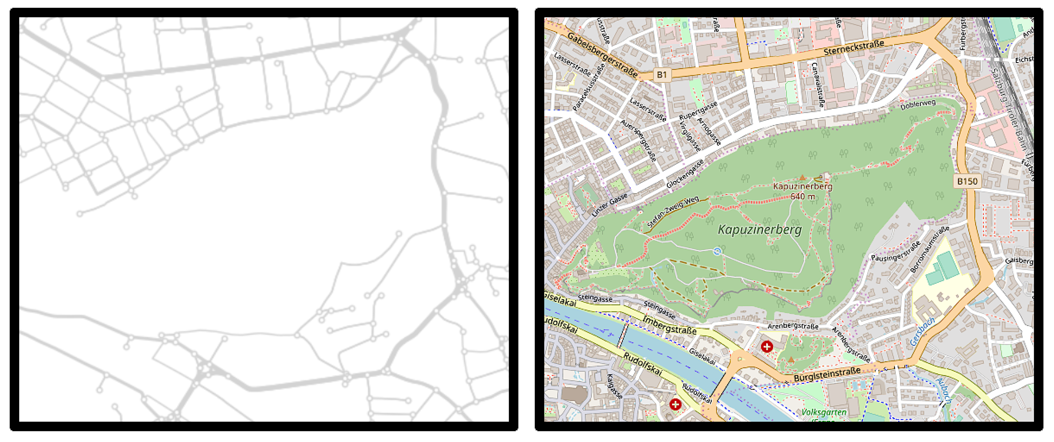
First, the investigated traffic system needs to be translated from a map to a spatial traffic network. This is done by interpreting all intersections and similar points of interest as nodes of a network. The road segments connecting them are the edges of the network. We used map data from OpenStreetMap (OSM) [
37], which we transformed using the OSMnx library [
38]. It can extract not only nodes and edges, but also relevant information about the roads (like speed limit and number of lanes). These are stored as edge attributes so they can be accessed during the simulation. A comparison between the map representation and the network representation of the city of Salzburg is shown in
Figure 2.
While some of the relevant information is already included in the map itself, other features need to be calculated. The most important ones are the fastest paths [
39] between all nodes in the network. They are used by the agents every time they make a decision about their path. Here, we could utilize the fact that the fastest paths are independent of the agent itself, and rather an intrinsic network property. By calculating them before the simulation and storing them as a node property, we can save a significant amount of computation time. If computer memory is an issue, it is also possible to not save the full information about all fastest paths. Calculating lists of nodes in reach within certain distances of each node is sufficient. For example, one could use driving distances of 100, 200, and 300 m. This facilitates computational speed. During the simulation, agents often search for a possible target node that is a certain distance away from them. By storing these possibilities as node properties, we minimize the amount of fastest path calculations that need to be performed. Note that fastest paths are calculated here as weighted shortest paths, where the weight is the average time necessary to move over the road represented as a network edge.
2.2. Generating Ways
A novel aspect of the presented model is that ways are not taken from origin–destination matrices, but calculated within the model based on mobility-behavior data. We imported data from “Österreich Unterwegs 2013/2014” [
40], a survey containing information about the mobility behavior of 18,000 Austrian respondents. Each respondent reported on two randomly selected days, leading to a dataset of roughly 36,000 days, distributed around the year. For each day, they described the number, length, and starting times of all trips they performed, which method of transportation they used, which car they used, and the reason for the trip (commute, leisure, or shopping). Information about the used cars includes the size of the car, divided into the three categories small (<1155 kg), medium, and large (>1550 kg), the year during which it was built, and the type of engine it uses (petrol, diesel, or other). This information, in combination with statistical data about the average emissions of cars built in a certain year [
41], was used to approximate the average fuel consumption of each car. Details on this process can be found in Reference [
13]. Note that the start and end point of the trips are not precisely known, but we do have access to demographic information about the respondents, like their age or their place of residence.
Using these empirical data as foundation, we generated mobility-behavior archetypes. Each archetype contains information about the performed trips, the used car, and an age bracket, but no specific start or end points. When investigating urban systems, it is viable to restrict the used archetypes to those originating from respondents living in the urban area in the scope, which was done for this study.
Once the network and the archetypes are set up, the actual agent-based simulation begins. Since we were interested in a full-scale model, we generated one agent for each inhabitant of the investigated city. They were positioned in the traffic network according to the population density of the area. If such information was available for the investigated system, the agents were separated into age brackets. Then they were assigned a random archetype corresponding to their age. They performed all trips given by the archetype with the respective mode of transportation. Choosing a target node for each trip is done by utilizing previously stored information about the distances between all nodes. If the agent, for example, needs to perform a trip of 1000 m, it can obtain a list of possible destinations with that distance from the node at which it is currently positioned. It then chooses a random viable node and loads or calculates the fastest path to that node. Each edge it crosses is used to store the relevant data of the trip, e.g., type of engine, consumed fuel, and time. Saving this information as an edge property rather than as agent property gives us the local resolution about resulting emissions. This is especially relevant for emissions with local effects, like NO.
In addition to the inhabitants of the investigated city, we also needed to include commuters coming from outside the city. They enter the city road network through the main and secondary roads connecting it with the surrounding network. Thus, nodes of the network where these connections would be placed in the total network were implemented as sources where commuters emerge. The number of commuters and their geographical origin are extracted from Reference [
42]. However, not all of these enter the city at the same time. This was modeled by a Gaussian distribution around 7:00 for the time of entry into the network. Consequently, only 68.27% of commuters enter the city at 7:00, while at 6:00 and at 8:00, 15.865% of them enter. Departure is carried out in a similar manner. The peak of distribution was set to 18:00, with 68.27% of agents exiting, and 15.865% exiting at 17:00 and 19:00.
The choice of which node to utilize for entering or exiting the city is based on the node properties and the coordinates of the commuter agent’s origin. Among the node properties were the speed limit at the connecting road, their connection to the other nodes, and their ‘highway’ tag in OSM. The latter served as an adjustment parameter [
43] for the free speed. Connected to the commuter’s origin and destination, influencing factors are directness and travelled distance. These serve as a proxy for the perceived difference in appeal for route choices.
The resulting paths, both from commuters and noncommuters, are only the first step in an iterative process. During the path selection of each agent, no information about congestion is available. Consequently, there is no direct interaction between agents. This interaction is later included in an iterative way by calculating the resulting congestion from the initial simulation run and using this information during the path selection in a second run. In effect, some agents avoid heavily congested roads. Previous work [
32] showed that most realistic results can be obtained by using just one such iterative step, with 10% of agents changing their path due to congestion, which is comparable to the value found by other studies of this behavior [
44].
Once realistic paths exist, we can then calculate the resulting congestion, as well as emissions with a local and temporal resolution.
2.3. Calculating Emissions
During the generation of the paths, the average fuel consumed by each car is already stored as an edge property based on the age and the size of the car, and the year in which it was built. Microscopic effects like speed dependency, ambient temperature, and cold start are only included through averages, not for individual cars. Other effects, like the state of traffic flow, cannot be included using a macroscopic perspective, and we need to calculate them in detail in each simulation run. Emissions of CO
, NO
, and others scale very differently in free-flowing, congested, or stop-and-go traffic [
45]. Thus, we need the state of the traffic flow on the respective road segment at the respective time.
In a first step, we need to calculate the capacity of each road segment. Hourly traffic capacity
[
46] can be calculated via [
47]
with
being the effective number of lanes.
is calculated starting from the actual number of lanes. If this number is unknown, it is possible to approximate values of 2.6 for roads wider than 7.5 m, 2.0 for roads between 7.5 and 5.5 m, and 0.8 for roads narrower than 5.5 m [
46]. For roads that are not one-way streets, this number of lanes is then halved, since only half of the traffic flow moves in the relevant direction there. The hourly capacity is then compared to the actual number of cars using this road for each hour. This leads to road-utilization factor
a:
The road-utilization factor can then be used to obtain the stage of traffic flow:
a smaller than 0.75 can be seen as free-flowing traffic,
a between 0.75 and 0.9 is congested traffic flow, and
a larger than 0.9 corresponds to stop-and-go traffic [
46].
For finding NO
emissions, we start out from fuel consumption calculated by the model. Using the European exhaust-emission standard [
48], we had access to estimates of NO
emissions for different engine types. Because of the mesoscopic perspective of the model, which is required for fast calculation, there is no precise information about the age of each car during the simulation run, and only their fuel consumption and type of engine are known. Therefore, we need to calculate NO
emissions from fuel consumption. This is not trivial. Due to the difference in EURO norms and the used engine type, there is no linear dependency. We based this calculation on the most common standard in the dataset (EURO 5) and the finding that especially diesel engines emit more nitrogen oxides in real-life conditions than they do under lab conditions. A study [
49] that investigated this phenomenon found that, under realistic conditions, diesel engines in compliance with the EURO 5 norm [
48] on average emit 3.5 times the emission limit. This gives us the required factors for EURO 5 diesel and petrol cars. Cars with higher fuel consumption gain an additional term for NO
emissions, linear to their increased fuel consumption. This approximation is sufficient for cars built in 2000 and earlier, but leads to errors for older cars. Fortunately, the investigated dataset contains only few such cars, so that the final result is still close to the measured value (see
Section 3).
Combining these estimates with factors that describe additional emissions caused by congestion or stop-and-go traffic [
45], we arrived at NO
emissions for every edge of the investigated traffic system.
2.4. Investigated Scenarios
In a baseline scenario, we depict the system as it currently is. Details about the investigated system are given in
Table 1.
In addition to the baseline scenario, we also investigated other scenarios in order to assess the potential of possible policies to reduce NO emissions.
As a first scenario, we looked into the replacement of a certain percentage of cars by electric cars. We scanned a large parameter space (2.5% to 20%), since the number of electric cars in the near future is currently unknown and difficult to predict. This scenario also serves as a method for evaluation purposes: We expect that replacing, e.g., 10% of cars with electric cars should lead to a decrease of nitrogen oxides by roughly 10%. Furthermore, this scenario can be used as a comparison for the effectiveness of other scenarios.
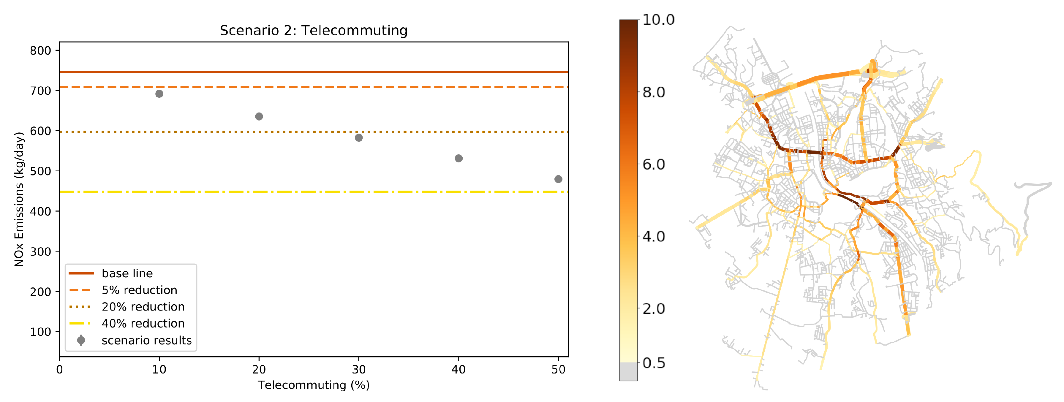
In a second scenario, we investigated a societal change: We increased the amount of telecommuting, a possible effect of digitalization. To represent this change in the model, we could remove a certain percentage of the trips that are performed for the reason of commuting. This information is already contained and calibrated to empirical data within the model. By removing up to 50% of work-related trips in increments of 10%, five subscenarios were simulated. These changes primarily affect rush hour, where most roads are congested. Thus, a nonlinear effect of emission reduction could be possible. Heavily used roads could also locally benefit more from this change.
Scenario 3 investigated a possible policy often discussed in the context of urban air quality. Here, we calculated the change resulting from replacing old diesel cars with cars that use a petrol engine. As variants of this scenario, we used the years 1995, 2000, 2005, and 2010, and substituted all diesel cars built prior. Additionally, a simulation with all diesel cars being replaced showed what a complete ban on these could yield. While possibly having a negative effect on CO emissions, such a change has the potential of significantly reducing NO emissions.
3. Results
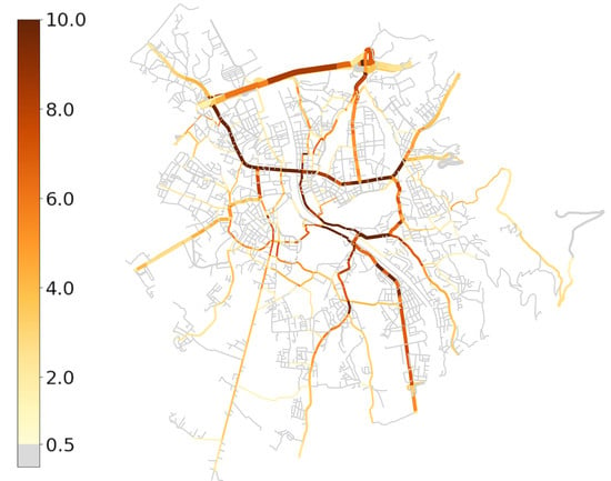
The baseline scenario leads to daily NO
emissions of 746 ± 7 kg. Their local distribution is shown in
Figure 3. Emissions mainly originate from the city center, and roads leading to and from the city center. We can also see bottlenecks where two roads merge into one, creating higher congestion and thus higher emissions.
In order to evaluate the results of the baseline scenario, we used statistical data about NO
emissions in Salzburg. The most recent data with regional resolution are available from the year 2006 [
50]. There, we found daily NO
emissions of roughly 2000 kg, of which about 680 kg were caused by PMT, and are thus within the scope of our model. Using the increase of cars in the city as a rough estimate for the increase in NO
emissions, we arrived at a value of 748 ± 37 kg per day (approximating the resulting error with 5%). Our simulations yielded 746 ± 7 kg, which is a satisfying result.
For evaluating the temporal and spatial resolution of the model, one has to rely on congestion data, since no high-resolution data about NO
emissions are available. Such a comparison is shown in
Figure 4. It shows simulated congestion during morning rush hour, compared to congestion data from Google Maps. A quantitative evaluation of the differences between real and simulated congestion of the used model [
32] showed average deviations of ±3%.
In addition, we could compare the results of the baseline scenario (
Figure 3) to an air-quality map from Reference [
51]. Note that this map shows NO
concentration, while we calculated emissions. Nevertheless, both maps show increased NO
on the highway, around the city center, and on roads connecting the highway and the city center.
Using this baseline result, we could then compare the different scenarios in terms of overall effect and localization of the effect. Results for Scenario 1, where we investigated the effects of an increase in the percentage of electric cars, are presented in
Figure 5. The left panel shows the overall reduction effect of this scenario for different intensities. The right panel shows an emission map of the investigated scenario with the highest intensity. As expected, the decrease in emissions was linear to the percentage of electric cars. This effect is evenly distributed throughout the city, since the replaced cars were chosen randomly. Results of this scenario cannot only be used to evaluate the model. They also give a point of reference in order to judge the effect of other scenarios.
In Scenario 2, we simulated an increase in telecommuting, effectively removing a certain percentage of commuting trips from the system. Results of this investigation are presented in
Figure 6. The effect is nonlinear: removing a certain amount of commuting trips reduces emissions more than randomly removing the same amount or trips without regarding the purpose of the trip. This has to do with the fact that commuting trips are very likely to occur on streets and during times where there is much congestion. Thus, removing those trips significantly alleviates congestion, leading to lower NO
emissions.
Older cars with a diesel engine produce more NO
per km than cars using a petrol engine. A viable way of reducing NO
emissions is hence to replace older diesel cars with petrol cars. Results of simulations where diesel cars built before a certain year were replaced by petrol cars of the same age are presented in
Figure 7. When this policy only affects cars built before 2000, the effects are relatively small (roughly 5% decrease in emissions). However, when the intensity of this policy is increased by also banning cars built in 2010 and older, the effect on NO
emissions is drastic. Banning diesel cars built before 2010 leads to a reduction of more than 50%. In a hypothetical case where all cars are replaced by petrol cars, NO
emissions would drop below 200 kg/day. Such a policy has also significant downsides. While the emission of NO
would decrease, CO
and other emissions might rise significantly. Even though the CO
emissions of petrol engines depend on many different factors, for example, engine size, on average they tend to emit more CO
than their diesel counterparts. Even though carbon dioxide has no direct local effects on air quality, it contributes to global warming and should therefore be minimized in a sustainable traffic system.
In terms of computation time, the model can operate significantly faster than real time: Simulating one day of traffic in Salzburg (over 100,000 citizens) takes approximately 20 min when utilizing 30 threads on a 3.4 GHz CPU. In contrast, other hybrid models optimized for quick computation calculate their results in real time [
15].
4. Discussion
In this study, we used a hybrid traffic model based on mobility-behavior data to calculate NO emissions resulting from PMT. We applied the model to the city of Salzburg and investigated several scenarios that included technological, sociological, and juridical changes to the traffic system, all within the same framework.
Evaluating the baseline scenario, which found daily NO
emissions of 746 ± 7 kg, showed good agreement with statistical data. The local distribution of the emissions also yielded realistic results. Emissions were concentrated in the city center and on large roads leading to it. On road segments with high congestion (bottlenecks), NO
emissions were also significantly higher. This is also in agreement with real-life measurements [
52].
Scenario 1 found that increasing the number of electric cars linearly decreases the resulting NO
emissions. However, achieving a high percentage of electric cars is currently not feasible [
53,
54,
55], even though there are many policies that try to promote using electric cars in an urban environment [
56,
57]. Furthermore, the overall environmental benefit of electric vehicles is difficult to assess [
58] and largely depends on the way the electrical energy is produced. It is thus possible that electric cars decrease local emissions at the cost of increasing global emissions.
Scenario 2 showed that telecommuting has great potential to decrease urban NO emissions. The nonlinear effect can be attributed to the fact that commuting trips primarily occur in places and at times where and when there is a lot of congestion. Removing them does not only remove direct emissions, but also effectively reduces emissions by other cars. As a further advantage of telecommuting, its adoption only needs minimal infrastructure or other forms of investment. It is already beginning to gain popularity due to digitization. Further promoting telecommuting might thus be a feasible way to reduce urban emissions in general.
Scenario 3 showed the biggest improvement in terms of NO emissions. It replaced old diesel cars with cars of the same age that use a petrol engine. However, this decrease in NO emissions came at the cost of increased CO emissions. The decrease in NO was smaller than the increase in CO. Nevertheless, it is difficult, if not impossible, to answer the question of whether a local benefit can outweigh a global drawback.
The presented model has various advantages compared to traditional state-of-the-art traffic models. Its foundation in mobility-behavior data makes it very flexible, so that diverse scenarios can be investigated. The used hybrid approach gives a mix of detail and calculation speed that is perfectly fitted for scenario evaluation. However, there are also some limitations to the model and possible expansions that could improve its predictive power. Since OD data are based on mobility behavior, we have no access to the target points of commuting trips, but have to generate them randomly at the correct distances. This has only a minor effect on overall emissions (since distances are correct), but might lead to an error in the local distribution of emissions. This could be remedied by including information about the workplace density of the investigated system. Unfortunately, such information is not available for every city. Including it would, hence, drastically limit the scope of the model. Further improvement could be to approximate these data from available OSM data. While the mesoscopic approach leads to fast computation times, it also has its downsides. For example, we lose some information about individual cars, like their exact age, during the simulation. For this investigation, it was possible to find a way to approximate it based on fuel consumption, which lead to satisfying results for NO emissions. This worked because the used dataset mainly contained cars in the EURO 5 and EURO 4 category. When investigating a different system, where the distribution of car ages is different, it might be beneficial to forgo some computational speed in order to microscopically calculate NO emissions. This could be a further improvement of the model.
In conclusion, the presented hybrid traffic model proved to be very well-suited for investigating NO emissions resulting from PMT. Its local resolution gives more insight than macroscopic models. It still remains fast enough to simulate whole cities on a 1:1 scale quicker than real time. Since it does not rely on OD data, it is possible to investigate scenarios that not only change certain properties of the cars, but also produce changes in the trips that people take. This provides us with a powerful tool to holistically investigate urban-traffic scenarios.


