Article

The Role of Synoptic Cyclones for the Formation of Arctic Summer Circulation Patterns as Clustered by Self-Organizing Maps

Korea Polar Research Institute, 26, Songdomirae-ro, Yeonsu-gu, Incheon 21990, Korea
*
Author to whom correspondence should be addressed.
Atmosphere 2019, 10(8), 474; https://doi.org/10.3390/atmos10080474
Submission received: 14 July 2019 / Revised: 12 August 2019 / Accepted: 16 August 2019 / Published: 19 August 2019
(This article belongs to the Special Issue Atmospheric Processes Shaping Arctic Climate)

Abstract

:
Contribution of extra-tropical synoptic cyclones to the formation of mean summer atmospheric circulation patterns in the Arctic domain (≥60° N) was investigated by clustering dominant Arctic circulation patterns based on daily mean sea-level pressure using self-organizing maps (SOMs). Three SOM patterns were identified; one pattern had prevalent low-pressure anomalies in the Arctic Circle (SOM1), while two exhibited opposite dipoles with primary high-pressure anomalies covering the Arctic Ocean (SOM2 and SOM3). The time series of their occurrence frequencies demonstrated the largest inter-annual variation in SOM1, a slight decreasing trend in SOM2, and the abrupt upswing after 2007 in SOM3. Analyses of synoptic cyclone activity using the cyclone track data confirmed the vital contribution of synoptic cyclones to the formation of large-scale patterns. Arctic cyclone activity was enhanced in the SOM1, which was consistent with the meridional temperature gradient increases over the land–Arctic ocean boundaries co-located with major cyclone pathways. The composite daily synoptic evolution of each SOM revealed that all three SOMs persisted for less than five days on average. These evolutionary short-term weather patterns have substantial variability at inter-annual and longer timescales. Therefore, the synoptic-scale activity is central to forming the seasonal-mean climate of the Arctic.

1. Introduction

Low-frequency atmospheric circulation modes in the Arctic (e.g., the Arctic Oscillation (AO), Dipole Anomaly (DA), etc.) have attracted much attention owing to their role as controlling factors in the spatiotemporal sea-ice variability [1,2,3]. This role can be investigated by various methods based on relatively more abundant atmospheric data sources, instead of with the ocean circulation patterns. Among the different seasons, the summer circulation pattern has received research focus because of its temporal proximity to the September sea-ice minimum [4,5,6,7,8,9]. However, preconditioning factors that occur during the winter and spring have also attracted much attention due to their importance in long-lead seasonal predictions [10,11,12].
The summer season is known to be the most synoptically active in the Arctic Ocean [13,14,15]. As high-latitude sea-ice and snow on land gradually disappear by seasonal warming, the meridional thermal contrast between the land and ocean preferentially forms the baroclinic frontal zone along the land–ocean boundary [16]. As a result, summer in the Arctic Ocean is stormier than the winter, which manifests as local cyclogenesis, as well as migratory mid-latitude cyclones [14]. Therefore, Arctic cyclones and their role in controlling sea-ice have been critical topics in understanding the Arctic summers [17,18,19].
From a scale interaction perspective, the Arctic is a singular region, where the zonal scales from synoptic to planetary merge, due to reduced length of latitudinal circles. If a strong synoptic cyclone/anticyclone persists or synoptic cyclones/anticyclones frequently pass near the pole, it can directly contribute to a low-frequency (i.e., monthly-to-seasonal) large-scale circulation pattern therein [13,14,20]. Serreze and Barrett [14] demonstrated that cyclone activity is dominant during the cyclonic summer sea-level pressure pattern by carrying out composite analysis and case investigation. On the other hand, Wernli and Papritz [20] revealed that the episodic synoptic anticyclones in the Arctic favor anticyclonic summer seasonal circulation that accounts for more summer sea-ice melting.
As described above, previous studies have suggested that the accumulation of synoptic events is relevant to generation of a preferred pattern of seasonal circulation in the Arctic, but none of them have attempted to investigate the quantitative contribution of synoptic cyclones to individual summer-mean large-scale circulation patterns in the Arctic. Accordingly, the detection and tracking of extra-tropical synoptic cyclones were carried out here to quantify cyclone activity and relate it with the summer-mean Arctic circulation patterns. We also strived to identify the summer-mean Arctic circulation patterns with a suitable pattern classification method. Among other methods, we adopted the self-organizing maps (SOMs) that have been proven to effectively distinguish representative patterns from large climate data sets [21,22,23,24]. Johnson [21] identified the continuum of El Niño–Southern oscillation (ENSO)-related sea-surface patterns. Lee and Feldstein [22] and Feldstein and Lee [23] used SOMs to distinguish the latitudinal shift of zonal-mean tropospheric jet streams in both hemispheres that are generally not distinguished by empirical orthogonal functions (EOFs). Reusch et al. [24] also suggested that the SOMs have the advantage of capturing both the known spatial patterns, such as the North Atlantic Oscillation (NAO), and their relative frequency occurrence, as compared to the EOFs. In addition, the SOMs have been used to distinguish patterns related to the variabilities of winter cold extremes over North America and Europe [25] and summer heat waves over the Northern Hemisphere [26]. These studies have concluded that clusters derived from the SOMs are more accurate and linearly independent as compared to those from the conventional hierarchical cluster analysis models.
This study is structured as follows. Section 2 provides descriptions of the data and analysis methods, including SOM clustering, detection, and tracking of synoptic cyclones and grid-cell representation of cyclone activity. Section 3 presents representative SOM patterns of Arctic large-scale surface circulation during summer and their inter-annual variations. Furthermore, this section also includes findings on synoptic cyclone activities, analyses relevant to cyclone development, and daily synoptic evolution of large-scale circulation in the Arctic in association with individual SOM patterns. Finally, summary and discussion are presented in Section 4.

2. Data and Methods

2.1. Data

We primarily used the atmospheric fields of the European Centre for Medium-Range Weather Forecasts Interim Reanalysis (ERA-Interim) dataset [27] with a 1.5° × 1.5° horizontal resolution during the boreal summer (June–July–August, JJA) seasons from 1979 to 2017. The SOM clustering algorithm utilized the daily mean sea-level pressure (MSLP) field with its climatological mean daily seasonal cycle removed. To smoothen the seasonal cycles, we considered the moving average of the daily climatological mean with a 1-2-1 filter; this is one of the weighting functions, where 0.5 is multiplied to the value for the current day, and 0.25 to the values for the day before and the next day in the moving average window. Further atmospheric analyses corresponding to SOM clusters were carried out using horizontal winds, temperatures, and geopotential heights between 850 hPa and 200 hPa. For storm detection, 6-hourly fields of the MSLP and 850-hPa relative vorticity were used as the input for the storm detection algorithm (see Section 2.3).

2.2. Self-Organizing Maps (SOMs)

In this study, the SOM algorithm was applied to the daily summer MSLP fields over the Arctic domain (north of 60° N) for the period from 1979 to 2017. The SOM algorithm is one of the common clustering methods that originate from neural networks (refer to the appendix in [28] for more details). Because it is based on the K-means clustering, it classifies data into a specified number of clusters through supervised machine learning. It differs from other clustering methods in that it relocates the resultant clustering patterns onto a one- or two-dimensional grid based on pattern similarities between the clusters [29]. This ad-hoc relocation allows the continuum of atmospheric circulation regimes to be fully described [21,28,30].
During training, individual data are partitioned into a particular SOM pattern, whereby the Euclidean distance between the SOM patterns and the data is at minimum. Here, it meant that each daily MSLP pattern was expected to have the best-matching SOM pattern. Naturally, the two patterns matched better when the predefined number of SOM patterns increased, but very large numbers of SOM clusters were less useful in clearly identifying the different physical modes represented by the data. Therefore, it is generally recommended to determine the optimal number of SOM patterns by considering the following two conditions: (1) The numbers of SOM patterns must be large enough to accurately capture the physical characteristics of the data and (2) it must be sufficiently small so that the clusters are distinctive from one another. Following the selection method described by [26], we computed (1) the average correlations between patterns in the daily fields and their best-matching SOM patterns [22] and (2) the distance between different cluster pairs (d: Ward’s linkage distance) using the following mathematical definition put forth by [26]:
d ( r , s ) = 2 n r n s ( n r + n s ) x ¯ r x ¯ s 2
where nr and ns are the number of elements in clusters r and s, respectively, and x ¯ r and x ¯ s are the centroid patterns of clusters r and s, respectively. The equation was obtained from the concept of Ward’s linkage that computes the merging cost of two clusters in a hierarchical cluster method. According to previous studies [26,31], this concept can be applied to measure the distinctiveness between clusters.
The SOM analyses were repeatedly carried out with varying SOM grids with sizes ranging from (2 × 1) to (10 × 1). Using the two criteria discussed before, the optimal number of SOM clusters was determined. As the number of SOM patterns increased, the mean pattern correlations (gray line) increased, while Ward’s linkage distances (black line) decreased (Figure 1). A significance test with Monte Carlo random resampling was performed to find out that the mean correlations between patterns for all SOM grids were statistically significant at the 5% level. However, the decreasing trend of Ward’s linkage distances was appreciably slower, when the SOM number increased from (3 × 1) to (4 × 1). This was an indication that the (3 × 1) grid could have the lowest optimal number that was just enough to yield distinct SOM patterns [26]. We, therefore, selected the (3 × 1) grid as it had the appropriate number of SOM patterns to classify the summer atmospheric circulation in the Arctic.
Limiting the SOM analysis to just three patterns did not allow sufficient resolution of geographical variations in regional synoptic features, which was in contrast with other studies that have reported more diverse SOM matrices with continuums of synoptic patterns [24,32]. More patterns can resolve details and delineate the evolution of the synoptic patterns. However, producing a higher number of synoptic patterns did not fit the purpose of this study as we aimed to elucidate the interaction between synoptic-scale high-frequency and large-scale low-frequency variabilities. The purpose of our study justified the selection of a low number of patterns, while following the selection method described by [26].

2.3. Cyclone Tracking and Gridding

For detection and tracking of extra-tropical cyclones, the method described by [33] was used, except for their criteria for tropical cyclone detection. Detecting cyclone centers in the Northern Hemisphere extra-tropics (north of 30° N) comprises the following three criteria: (1) A local maximum of the 850-hPa relative vorticity larger than 2.0 × 10⁻⁵ s−1 within each 11 × 11 grid window, (2) the closest local minimum of the MSLP within a 400-km radius of the local vorticity maximum found via (1), and (3) the increase in MSLP by at least 15 Pa in all directions within a 500-km distance from the local pressure minimum found using (2). Followed by detection of all cyclone centers, the temporal movement of detected cyclones was tracked by the technique to determine the most probable migrated position at the next step in time. The procedure had three steps as follows: (1) Detected cyclone centers were selected within the circular tracking boundary (radius: 750 km) from a cyclone center at the previous step in time. (2) In case of the selection of a center within the boundary, it was considered to be the cyclone position after migration. If there existed multiple centers, the algorithm prioritized the nearest center present in the front semicircle toward the moving direction of the cyclone, but if there were none in the front semicircle, the nearest one was selected, regardless of the direction. If no cyclones were detected within the boundary, the algorithm stopped tracking that cyclone. (3) Among the output data of cyclone tracking, cyclones with lifetimes shorter than 1.5 days were discarded. The remaining cyclones were then tracked and were archived in the final cyclone tracking database.
Transforming cyclone tracks into grid-cell counts has its merits for clearly presenting the distribution of cyclone activity [34]. Due to singularity near the pole, we constructed equidistant grid-cells that were 500 km × 500 km and centered on the pole, rather than the conventional latitude–longitude grid-cells. The gridded spatial distribution was constructed for each summer. The gridded data were then used to reveal climatological or composite anomalies. In this study, the grid-cell cyclone frequency was depicted for the spatial distribution of cyclone activity, which is defined by counting a cyclone only once when it enters the grid.

3. Results

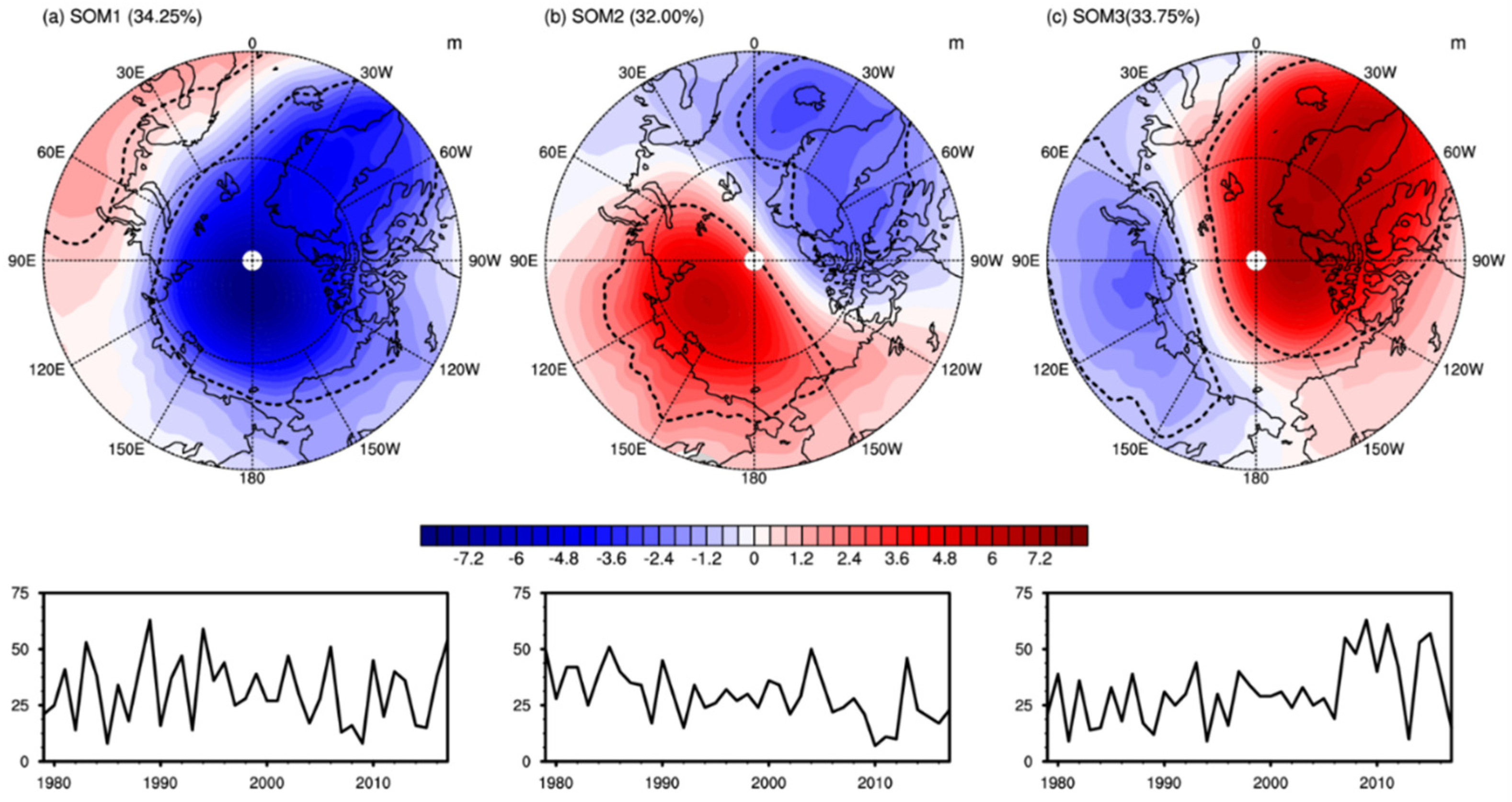
3.1. SOM Patterns for the Summer MSLP in the Arctic

Figure 2 shows spatial patterns of three SOMs (SOM1, SOM2, and SOM3) and time series of their individual occurrence frequencies in each summer (i.e., JJA). The frequency of occurrence was obtained by counting the number of days showing the best match with a particular SOM pattern. It was observed that the three SOMs were almost evenly divided over the summer days; this was indicative of three major patterns in the Arctic summer MSLP. Here, SOM1 showed that the negative MSLP anomaly prevailed over the Arctic Ocean, except over northern Europe, and its frequency of occurrence largely fluctuated from year to year over the whole study period (Figure 2a). This pattern resembled the polar branch of the AO during its positive phase [2,5].
SOM2 represented the DA between the Atlantic Arctic sector and the Eurasian Arctic–Canada Basin sector (Figure 2b). Although this summertime DA of the SOM2 had a node slightly rotated counterclockwise, as compared to the summertime DA as shown in Figure 2d in [3] derived from the empirical orthogonal function (EOF) analysis, it is reasonable to say that our SOM2 DA was qualitatively similar to the negative phase of the DA reported by [3]. As compared to other SOM patterns, SOM2 had a relatively lower inter-annual variability, as well as a slightly decreasing trend.
By contrast, SOM3 appeared to have a DA-like pattern that took on the shape opposite to that seen in case of SOM2, but the node of the DA now existed along the Eurasian Arctic seas (Figure 2c). It was qualitatively similar to the positive phase of the DA reported by [3] and was related to the reduction in the Arctic sea-ice; this, in turn, represented the anomalous anticyclonic patterns prevalent over the Canadian Basin [6,9,20]. Interestingly, an abrupt increase since 2007 was observed in the time series of the SOM3 occurrence frequency, when a large sudden decrease occurred in the time series of Arctic sea-ice expanse.
The SOM-based clustering patterns in the Arctic MSLP had both similarities and discrepancies in their shapes as compared with the previous EOF-based circulation patterns. The SOM analysis is known to have advantages over the EOF analysis, such as its capability to yield asymmetric features and extract complex patterns [35]. Therefore, it is speculated that the three SOM patterns reflect the real climate regimes in the summer surface atmospheric circulation of the Arctic.

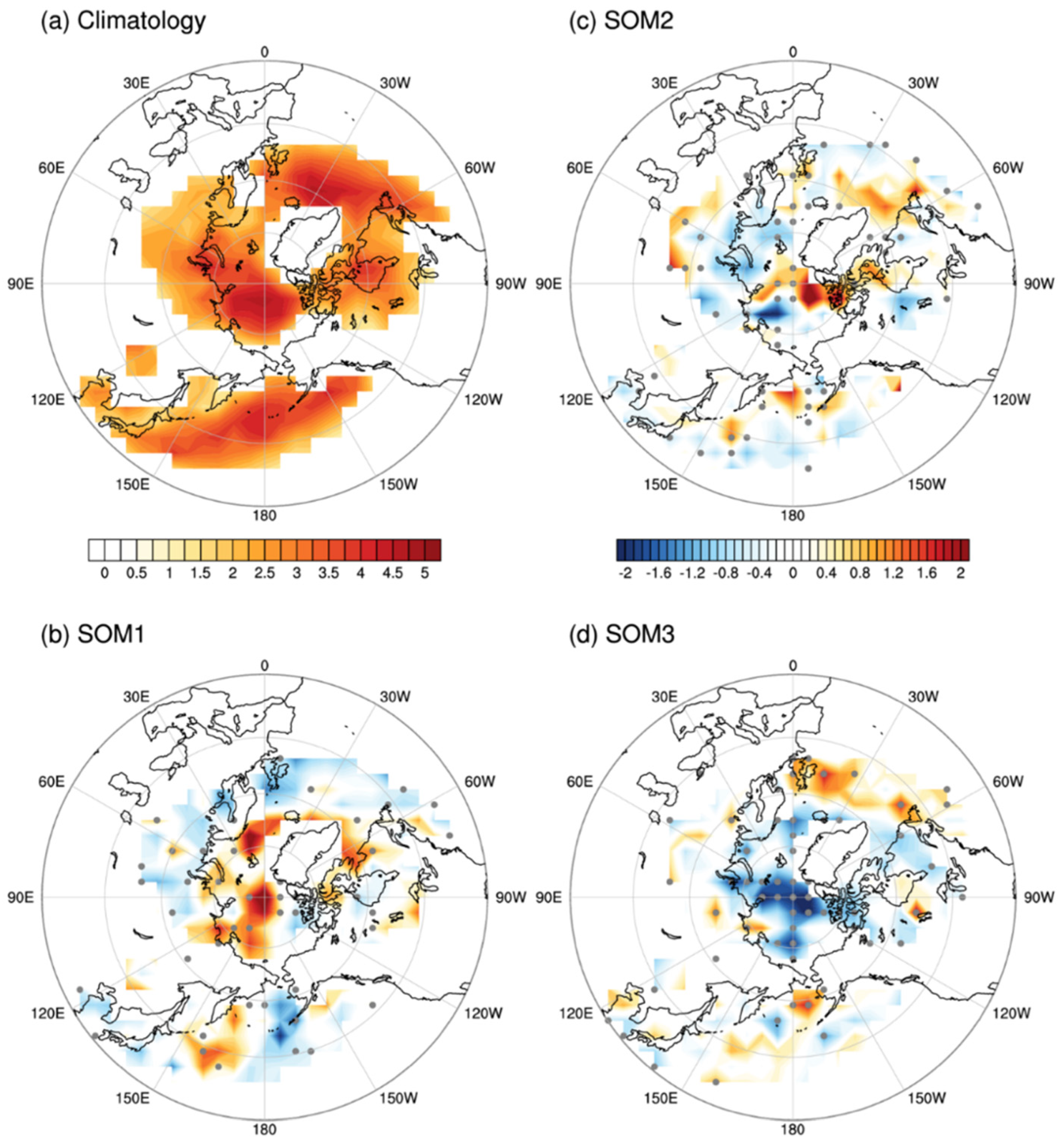
3.2. Cyclone Activities Associated with the SOMs

Based on the three Arctic surface circulation regimes (SOM1–3), we have tried to identify the role of synoptic cyclone activity in the formation of individual circulation regimes. First, the composite maps of grid-cell cyclone frequency were constructed for the five years that had the highest occurrence frequencies of individual SOMs. To focus on the inter-annual variability of the MSLP in relation to the Arctic cyclone activity, we used a detrended time series for composite analysis. Table 1 lists the selected five years for each SOM pattern. The chosen five years for composite analysis corresponded to the top 12.5th percentile during the 39 years from 1979 through 2017. The results were observed to be insensitive to the number of years chosen from the first four (10th percentile) to six (15th percentile) years (data not shown).
Figure 3 depicts the resultant climatological distribution of extra-tropical cyclones during the period from 1979 to 2017 (3a), as well as the composite anomalies associated with the first five years with the highest individual SOMs (3b–d). According to [14], summer cyclones in the Arctic can develop due to enhanced thermal contrast between land and the Arctic Ocean. Consistent with their study, the activity core over the Arctic Ocean was clearly observed in our results as well, in addition to two mid-latitude cores in the North Pacific and North Atlantic Oceans (Figure 3a).
The composite anomalies in grid-cell cyclone frequencies in the SOM1 high years show a remarkable increase over the central Arctic Ocean and Greenland–Norwegian seas (Figure 3a). Meanwhile, the cyclone frequencies in the mid-latitude North Atlantic and the Bering Sea, which are regions of cyclone activity, are climatologically frequent; occurrence tended to decrease in the SOM1 years of high frequency. Considering the distribution of cyclone frequencies, the seasonal formation of SOM1 pattern was closely linked to the higher synoptic cyclone activity over the central Arctic Ocean and Greenland–Norwegian seas. The MSLP anomalies associated with the SOM2 pattern were characterized by the dipole pattern between the Eurasian Arctic–Canadian Basin sector and the Atlantic–Arctic sector (Figure 2b). Consistent with the circulation pattern, the composite anomalies in the grid-cell cyclone frequencies also showed a dipole with positive anomalies around Greenland and the Canadian Arctic Archipelago and negative anomalies in the Eurasian Arctic side during the SOM2 high years (Figure 3c). During the SOM3 high years, the overall cyclone frequencies over the Arctic Ocean were significantly reduced (Figure 3d). Meanwhile, the cyclone frequencies in the mid-latitude North Atlantic and the Bering Sea increased, but those cyclones seemed to seldom migrate into the Arctic Ocean. As the SOM3 pattern in the dipole was dominated by high pressure in the Arctic Ocean area (Figure 2c), it matched well with the SOM3 composite anomalies in the grid-cell cyclone frequencies.
A comparison of spatial patterns (Figure 2 vs. Figure 3) qualitatively displayed the relevance of synoptic cyclone activity to the formation of summer-mean circulation patterns in the Arctic. To statistically quantify the contribution of cyclones over the entire analysis period, a temporal correlation analysis was performed using the time series of cyclone activity indices (i.e., frequency, duration, central pressure, and accumulated cyclonic energy (ACE) [36,37] and summer-mean MSLP. The positive and negative core areas of individual SOMs were selected to construct the time series, which were based on the anomaly patterns depicted in Figure 2. The frequency was constructed by counting the number of cyclones passing through the core area, while the duration counted all six-hourly cyclone positions for all cyclones within the core area. This was then divided by four to express in units of days. The mean intensity is defined as the average of six-hourly central pressure data for all six-hourly cyclone positions within the core area.
The resultant correlation coefficients reveal that, among the indices, the central pressure, which is among the indicators of cyclone intensity, has the highest absolute correlations for all core areas of the SOM patterns with statistical significance of 5% level (Table 2). This result stands to reason because the cyclone’s central pressure itself is a variable equivalent to the MSLP. Therefore, the overall cyclone intensity is the most effective determiner of the seasonal-mean MSLP anomaly pattern in the Arctic. As another indicator showing the cyclone intensity, the ACE for each core area was calculated by the sum of squared maximum winds, when the cyclone center was located in the core area. The ACE also had a significant correlation, except for the negative core area of the SOM3. Overall, duration was the second most-effective determiner; although in some cases, correlations with the ACE exceeded those with the duration (e.g., the positive core area of the SOM1 and the negative core area of the SOM2); frequency played a significant role, which was almost equivalent to the duration (e.g., the negative core area of SOM2 and the positive core area of SOM3). Over the negative core area of SOM3, none of the indices, except for the central pressure, were effective in the formation of the seasonal-mean MSLP anomaly. However, this area did not have a primary core, but only a secondary one in that SOM pattern (Figure 2).

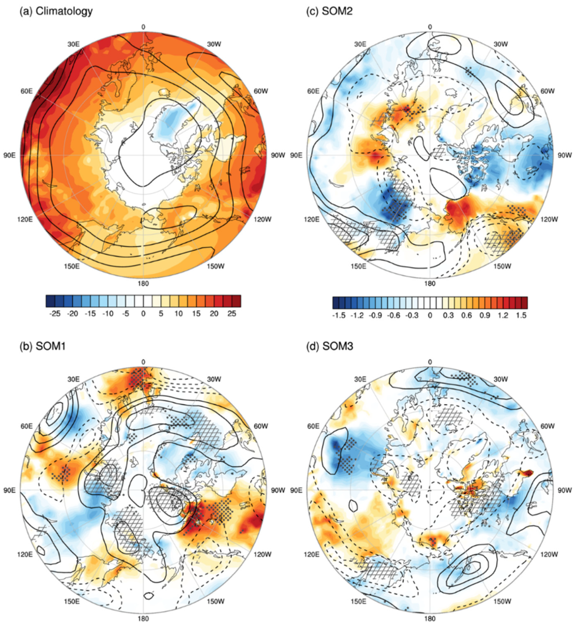
3.3. Large-Scale Fields Relevant to the Cyclone Activity Forming Each SOM

We have shown that the spatiotemporal variation in extra-tropical cyclones contributes significantly to the formation of the summer-mean circulation pattern in the Arctic. Now it is necessary to understand the large-scale atmospheric fields to provide a background for their spatiotemporal variation. As a primary energy source for extra-tropical cyclones, the baroclinic instability is modulated by the changes in the meridional temperature gradient (the vertical shear of horizontal winds), thus we displayed the composite anomalies of the 200-hPa zonal wind (U200) and skin temperature (Ts) for the first five years with the highest individual SOMs (Figure 4). As an indicator of baroclinicity, the Eady growth rate and the vertical shear of zonal winds (200 minus 850 hPa) were also investigated, but the U200 has been shown only because it primarily determines both the Eady growth rate and the vertical wind shear. In the climatological pattern, the summer Ts around the Arctic Circle showed a large gradient between land and ocean, and the higher speed of U200 appeared along the mid-latitude jets (Figure 4a).
For the SOM1 high years (Figure 4b), warm Ts anomalies were distributed over Western Europe, Ural Mountains, Northern Territories of Canada, and far-eastern Russia, while weaker cold Ts anomalies were located north of those warm Ts anomalies. This indicated a stronger meridional temperature gradient, and thus, the formation of positive U200 anomalies (i.e., the larger vertical shear of zonal winds) north of the warm Ts anomalies. The faster U200 prevailed over the Arctic Ocean rim and the northern North Atlantic Ocean, leading to more frequent poleward migration of synoptic cyclones from the North Atlantic Ocean, as well as local cyclogenesis in the Arctic. These results were observed for the SOM1 high years and can be expected because the areas of faster U200 coincided with those with climatologically frequent cyclone activity, such as the northern Russian coast, Canadian Arctic Archipelago, and northern North Atlantic Ocean (Figure 3a).
Furthermore, for the SOM2 high years (Figure 4c), there were two Arctic areas with warm Ts anomalies: One from the Barents Sea towards the Taymyr Peninsula in the far north of Russia and the other over Alaska. There were two Arctic areas as well with cold Ts anomalies: One over northeastern Russia and the other over the Canadian Arctic Archipelago. However, the anomalies were only statistically significant over the Barents Sea and northeastern Russia. Accordingly, the statistically significant U200 anomalies were also appreciable around those regions. Although not as clear as for the composite anomalies in the SOM1 high years, these overall U200 weakening effects surrounding the Eurasian Arctic could contribute to less cyclone activity therein (Figure 3c).
Lastly, composite anomalies in the SOM3 high years partly showed a state opposite to those in the SOM1 high years (Figure 4d). This meant that there was a reduced meridional temperature gradient and slower U200 anomalies surrounding the Arctic Ocean rim and the northern North Atlantic Ocean, resulting in less cyclone migration from the North Atlantic Ocean, as well as an overall reduced cyclogenesis in the Arctic (Figure 3d).

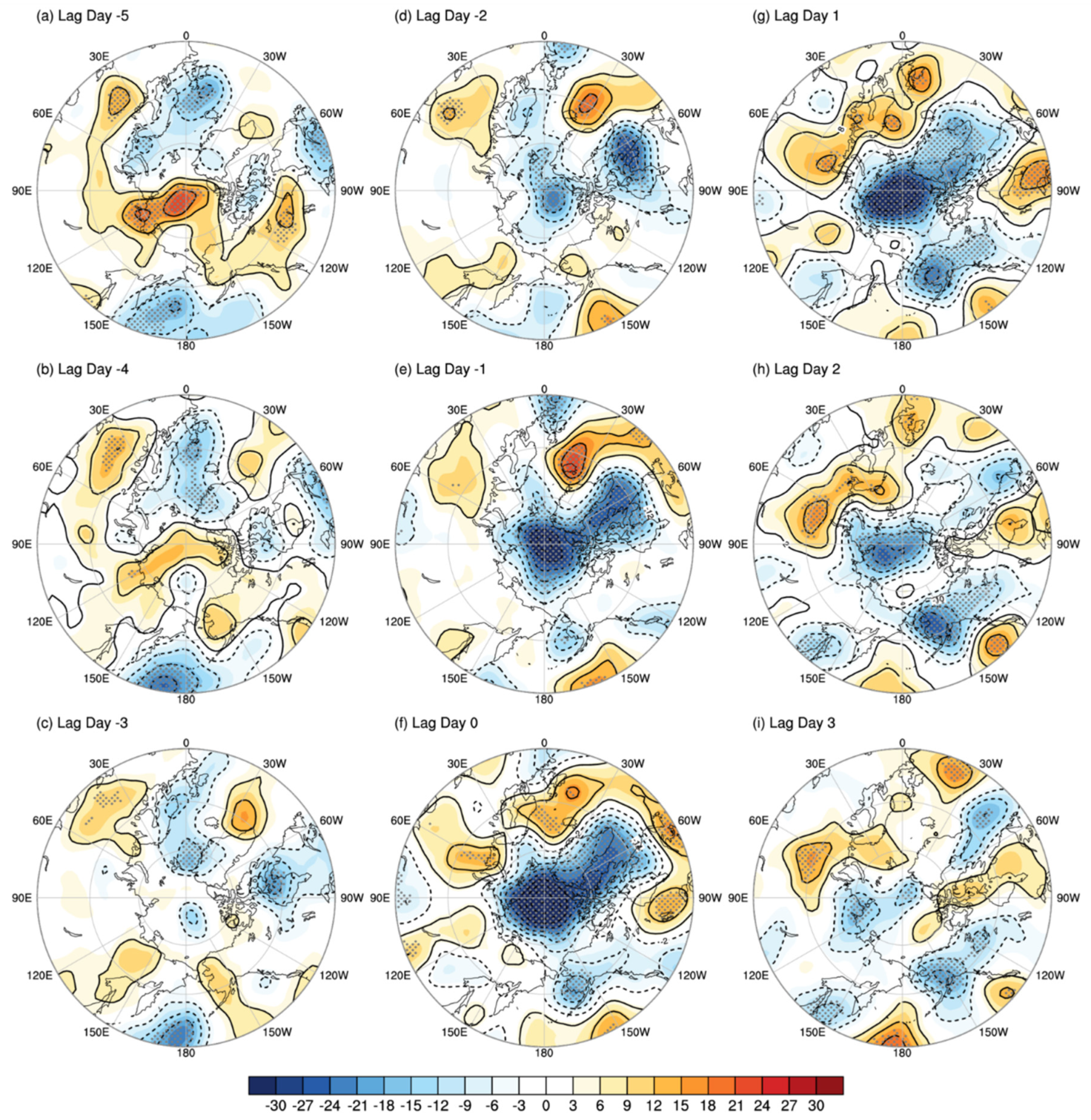
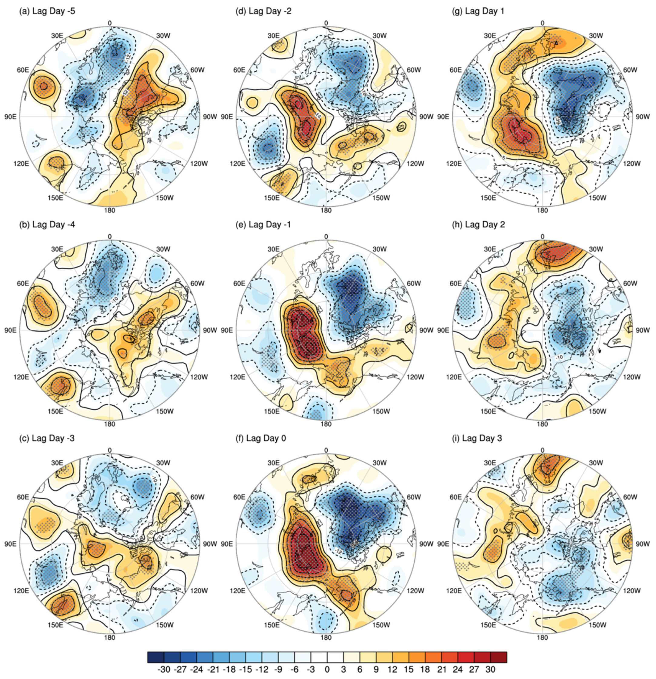
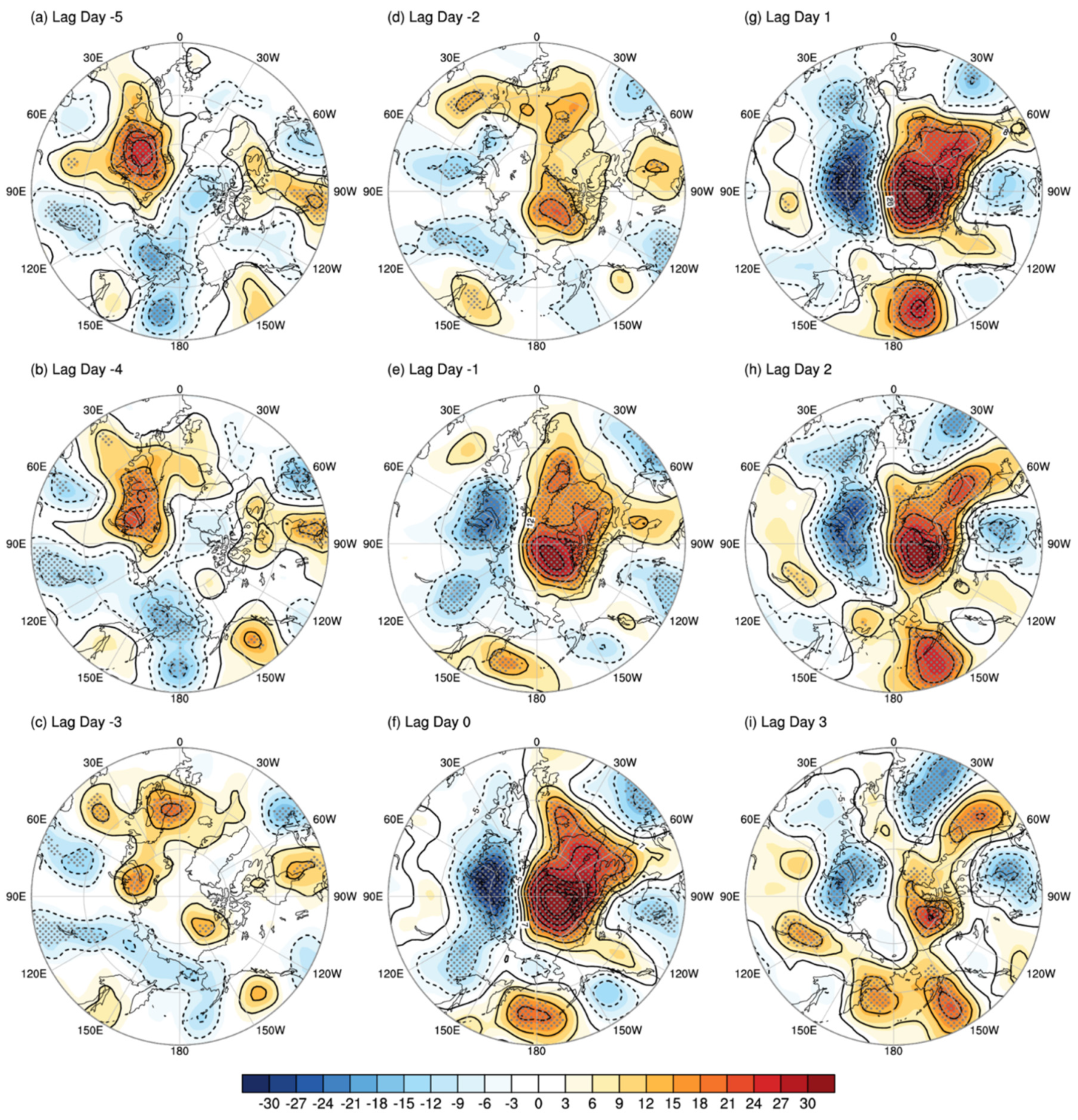
3.4. Synoptic Evolution Associated with the SOMs

Due to the significant role of synoptic cyclones in the formation of summer-mean Arctic circulation patterns as clustered by the SOMs, it was informative to characterize the generalized daily evolution of synoptic activity for each SOM by constructing lead–lag composites. Although all 3588 days had to be classified into one of the SOM patterns, the similarity between the daily anomaly field and the SOM pattern varied from day to day. Therefore, if there are consecutive days with one SOM pattern, the best-matching day needs to be determined as lag 0 days among them to perform the lead–lag composite analysis. Among the consecutive days with the same SOM, we selected the day with the smallest root mean square error (RMSE) between the daily MSLP anomaly pattern and the SOM pattern. Through this process, we identified 109 events for the SOM1, 112 for the SOM2, and 114 for the SOM3, for the period from 1979 to 2017. Before constructing lead–lag composites, 15-day moving averages were subtracted from the daily data to focus only on the synoptic-scale variability. In Figure 5, Figure 6 and Figure 7, the daily evolutions for individual SOMs are shown with the 500-hPa geopotential height (H500).
The composite daily evolution associated with the 109 SOM1 events (Figure 5) showed how the prevailing low-pressure system takes up the entire Arctic Ocean at lag day 0 (Figure 5f). From lag day −5 to −2 (Figure 5a–c), the northward migrating low-pressure composite was detected in the Norwegian Sea and the East Siberian Sea, where only the former was statistically significant at the 5% level. They quickly replaced the preexisting high-pressure composite in the Central Arctic Ocean and got stronger until lag day 0. Meanwhile, another low-pressure composite developed around Quebec, Canada and extended northward. Eventually, a massive low-pressure composite occupied the Arctic Ocean towards Greenland (Figure 5f). The low-pressure composite in the Arctic Ocean was sustained significantly until lag day 2 (Figure 5h) and then weakened at lag day 3 (Figure 5i).
Figure 6 shows the composite daily evolution of the 112 best-matching events for SOM2. At lag day −5, a reversed dipole analogous to the SOM3 pattern existed (Figure 6a). This pattern was quickly transformed to the incipient stage of SOM2 during lag day −4 to −3 by development of a high-pressure composite over the Taymyr Peninsula and the Laptev Sea and the development of a low-pressure composite in-and-around Greenland (Figure 6b,c). These two opposite pressure systems further developed and then the SOM2-like dipole pattern prevailed in the Arctic from lag day −2 to lag day 1 (Figure 6d–g). After the SOM2 event, the low-pressure system tended to prevail over the Arctic Ocean (Figure 6h,i). Based on the subjective comparison of the composite evolutions between the two SOMs, the SOM2 event seemed to last shorter than the SOM1 event. The calculation of the e-folding timescales of the SOM1 and SOM2 (i.e., 4.4 and 3.6, respectively) supports our conjecture.
Lastly, the composite daily evolution is presented in Figure 7 for the 114 best-matching events for SOM3. Similar to SOM2, there existed a dipole opposite to the SOM3 pattern at lag day −5 (Figure 7a). The high-pressure composite around the Barents–Kara seas was pronounced, but it weakened within three days (Figure 7b–d). The low-pressure composite gradually developed and replaced the high in the far north of Russia around the Kara–Laptev seas (Figure 7d–f), while the high-pressure composite began to separately develop in the Beaufort Sea and the Norwegian Sea at lag day –2, which merged into one broad high pressure system that expanded towards the central Arctic Ocean at lag day 0 (Figure 7c–f). The SOM3 event showed persistence after the peak day until lag day 3 (Figure 7g–i).
It should be noted that the composite daily synoptic evolutions discussed above do not necessarily mean that all individual events follow those simplified conceptual evolutions. Considering the noisy day-to-day evolution of synoptic systems in the extra-tropics, it is natural to view the information here in a statistical perspective. Except for the core systems in the Arctic Circle around the lag day 0, the other statistically significant composite anomalies in the marginal area that look like well-shaped synoptic systems should be less similar to the individual daily anomalous synoptic patterns. Nevertheless, the statistically significant anomalies should be presented even in the marginal areas only if similar anomalies frequently appeared around those areas. Therefore, the composite daily synoptic evolution of a particular SOM could be considered as the representative arrangement of extra-tropical synoptic systems.

4. Discussion and Conclusions

The formation of monthly-to-seasonal atmospheric circulation patterns observed using low-frequency modes in the Arctic has been extensively studied in terms of their influences on the Arctic climate and sea ice [1,2,3,4,5,6,7,8,9]. Studies have shown that the activity of synoptic cyclones is more prevalent during summer in the Arctic Ocean [13,14,15]; furthermore, it has been suggested that they potentially contribute to seasonal-mean Arctic climate [13,14,20]. Our results add to literature on the quantitative contribution of synoptic cyclone activity to the amplitude of seasonal-mean anomalies in individual activity cores of the three dominant Arctic summer circulation patterns as clustered by the SOM method (Table 2). We have also confirmed that the spatiotemporal distribution of synoptic cyclones in the Arctic domain is a major controlling factor for the Arctic summer circulation patterns (Figure 2 and Figure 3). Furthermore, the summer cyclone activities in the central Arctic Ocean are enhanced only for the circulation pattern (e.g., SOM1) that occurs at the land–Arctic Ocean boundary area with enhanced baroclinicity (i.e., increased meridional temperature gradient) and is co-located with the climatological major cyclone pathways (Figure 3 and Figure 4).
The composite daily synoptic evolutions demonstrated the generalized formation processes and elucidated the timescales of the three SOM patterns of atmospheric circulation in the Arctic well (Figure 5, Figure 6 and Figure 7). Although their evolutionary pattern has been revealed with the high-pass filtered data by retaining only the synoptic-scale variability, it is expected to be almost consistent with patterns obtained from the unfiltered daily data. The reason for this expectation is that the evolutionary SOM patterns depicted in Figure 5, Figure 6 and Figure 7 are based on a timescale of a couple of days (i.e., within the synoptic-scale variability) with e-folding times of 4.4, 3.6, and 3.6 days for the SOM1–3, respectively. According to previous literature, these short timescale weather evolutions have substantial variability at the inter-annual and longer timescales beyond the climate noise [38,39,40]. Therefore, it is reasonable to contend that the summer-mean Arctic circulation patterns reflect the accumulation of short timescale events, such as synoptic cyclones or anticyclones in the region as studied by [20].
The Arctic is not an isolated region; in fact, it has Northern Hemispheric high-latitude components of the global climate system that actively interact with components of lower latitudes [41,42,43]. Therefore, the inter-annual and longer-timescale changes in the Arctic circulation patterns should be understood in the context of global climate variability. Further studies are necessary to investigate the different forms of global climate variability that may provide relevant teleconnections for the different summer climatic states in the Arctic.

Author Contributions

Individual authors contributions are summarized as follows: “Conceptualization, J.-H.K.; Methodology, M.-H.L.; Formal Analysis, M.-H.L.; Writing—Original Draft Preparation, M.-H.L. and J.-H.K.; Writing—Review and Editing, J.-H.K.; Visualization, M.-H.L.; Supervision, J.-H.K.; Project Administration, J.-H.K.; Funding Acquisition, J.-H.K.”

Funding

This study was funded by the Korea Polar Research Institute (KOPRI) project, entitled ‘Development and Application of the Korea Polar Prediction System (KPOPS) for Climate Change and Weather Disasters’ (KOPRI, PE19130).

Acknowledgments

The authors are grateful to the editor and two anonymous reviewers.

Conflicts of Interest

The authors declare no conflict of interest.

References

  1. Rigor, I.G.; Wallace, J.M.; Colony, R.L. Response of sea-ice to the Arctic oscillation. J. Clim. 2002, 15, 2648–2663. [Google Scholar] [CrossRef]
  2. Rigor, I.G.; Wallace, J.M. Variations in the age of Arctic sea-ice and summer sea-ice extent. Geophys. Res. Lett. 2004, 31, L09401. [Google Scholar] [CrossRef]
  3. Wang, J.; Zhang, J.; Watanabe, E.; Ikeda, M.; Mizobata, K.; Walsh, J.E.; Bai, X.; Wu, B. Is the Dipole anomaly a major driver to record lows in Arctic summer sea ice extent? Geophys. Res. Lett. 2009, 35, L05706. [Google Scholar] [CrossRef]
  4. Ogi, M.; Wallace, J.M. Summer minimum Arctic sea ice extent and the associated summer atmospheric circulation. Geophys. Res. Lett. 2007, 109, D20114. [Google Scholar] [CrossRef]
  5. Ogi, M.; Yamazaki, K. Trends in the summer northern annular mode and Arctic sea ice. SOLA 2010, 6, 41–44. [Google Scholar] [CrossRef]
  6. Ogi, M.; Wallace, J.M. The role of summer surface wind anomalies in the summer Arctic sea ice extent in 2010 and 2011. Geophys. Res. Lett. 2012, 39, L09704. [Google Scholar] [CrossRef]
  7. Screen, J.A.; Simmonds, I.; Keay, K. Dramatic interannual changes of perennial Arctic sea ice linked to abnormal summer storm activity. J. Geophys. Res. 2011, 116, D15105. [Google Scholar] [CrossRef]
  8. Knudsen, E.M.; Orsolini, Y.J.; Furevik, T.; Hodges, K.I. Observed anomalous atmospheric patterns in summers of unusual Arctic sea ice melt. J. Geophys. Res. 2015, 120, 2595–2611. [Google Scholar] [CrossRef] [Green Version]
  9. Ding, Q.; Schweiger, A.; L’Heureux, M.; Battisti, D.; Po-Chedley, S.; Johnson, N.; Blanchard-Wrigglesworth, E.; Harnos, K.; Zhang, Q.; Eastman, R.; et al. Influence of high-latitude atmospheric circulation changes on summertime Arctic sea ice. Nat. Clim. Chang. 2017, 7, 289–295. [Google Scholar] [CrossRef]
  10. Kapsch, M.; Graversen, R.G.; Tjernström, M. Springtime atmospheric energy transport and the control of Arctic summer sea–ice extent. Nat. Clim. Chang. 2013, 3, 744–748. [Google Scholar] [CrossRef]
  11. Park, H.-S.; Lee, S.; Kosaka, Y.; Son, S.-W.; Kim, S.-W. The impact of Arctic winter infrared radiation on early summer sea ice. J. Clim. 2015, 28, 6281–6296. [Google Scholar] [CrossRef]
  12. Williams, J.; Tremblay, B.; Newton, R.; Allard, R. Dynamic preconditioning of the minimum September sea-ice extent. J. Clim. 2016, 29, 5879–5891. [Google Scholar] [CrossRef]
  13. Zhang, X.; Walsh, J.E.; Zhang, J.; Bhatt, U.S.; Ikeda, M. Climatology and interannual variability of Arctic cyclone activity: 1948–2002. J. Clim. 2004, 17, 2300–2317. [Google Scholar] [CrossRef]
  14. Serreze, M.C.; Barrett, A.P. The summer cyclone maximum over the central Arctic ocean. J. Clim. 2008, 21, 1048–1065. [Google Scholar] [CrossRef]
  15. Orsolini, Y.J.; Sorteberg, A. Projected changes in Eurasian and Arctic summer cyclones under global warming in the Bergen climate model. Atmos. Ocean. Sci. Lett. 2009, 2, 62–67. [Google Scholar] [CrossRef]
  16. Crawford, A.D.; Serreze, M.C. A new look at the summer Arctic frontal zone. J. Clim. 2015, 28, 737–754. [Google Scholar] [CrossRef]
  17. Mesquita, M.; Kvamstø, N.G.; Sorteberg, A.; Atkinson, D.E. Climatological properties of summertime extra-tropical storm track in the Northern Hemisphere. Tellus A. 2008, 60, 557–569. [Google Scholar] [CrossRef]
  18. Simmonds, I.; Rudeva, I. The great Arctic cyclone of August 2012. Geophys. Res. Lett. 2012, 39, L23709. [Google Scholar] [CrossRef]
  19. Semenov, A.; Zhang, X.; Rinke, A.; Dorn, W.; Dethloff, K. Arctic intense summer storms and their impacts on sea ice—A regional climate modeling study. Atmosphere 2019, 10, 218. [Google Scholar] [CrossRef]
  20. Wernli, H.; Papritz, L. Role of polar anticyclones and mid-latitude cyclones for Arctic summertime sea-ice melting. Nat. Geosci. 2018, 11, 108–113. [Google Scholar] [CrossRef]
  21. Johnson, N.C. How many ENSO flavors can we distinguish? J. Clim. 2013, 26, 4816–4827. [Google Scholar] [CrossRef]
  22. Lee, S.; Feldstein, S.B. Detecting ozone- and greenhouse gas-driven wind trends with observational data. Science 2013, 339, 563–567. [Google Scholar] [CrossRef]
  23. Feldstein, S.B.; Lee, S. Intraseasonall and interdecadal jet shift in the Northern Hemisphere: The role of warm pool tropical convection and sea ice. J. Clim. 2014, 27, 6497–6518. [Google Scholar] [CrossRef]
  24. Reusch, D.B.; Alley, R.B.; Hewitson, B.C. Relative performance of self-organizing maps and principal component analysis in pattern extraction from synthetic climatological data. Polar Geogr. 2005, 29, 188–212. [Google Scholar] [CrossRef]
  25. Bao, M.; Wallace, J.M. Cluster analysis of Northern Hemisphere wintertime 500-hPa flow regimes during 1920–2014. J. Atmos. Sci. 2015, 72, 3597–3608. [Google Scholar] [CrossRef]
  26. Lee, M.-H.; Lee, S.; Song, H.-J.; Ho, C.-H. The recent increase in the occurrence of a boreal summer teleconnection and its relationship with temperature extremes. J. Clim. 2017, 30, 7493–7504. [Google Scholar] [CrossRef]
  27. Dee, D.P.; Uppala, S.M.; Simmons, A.J.; Berrisford, P.; Poli, P.; Kobayashi, S.; Andrae, U.; Balmaseda, M.A.; Balsamo, G.; Bauer, P.; et al. The ERA-Interim reanalysis: Configuration and performance of the data assimilation system. Quart. J. R. Meteorol. Soc. 2011, 137, 553–597. [Google Scholar] [CrossRef]
  28. Johnson, N.C.; Feldstein, S.B.; Tremblay, B. The continuum of Northern Hemisphere teleconnection patterns and a description of the NAO shift with the use of self-organizing maps. J. Clim. 2008, 21, 6354–6371. [Google Scholar] [CrossRef]
  29. Kohonen, T. Self-Organizing Maps, 3rd ed.; Springer: Berlin, Germany, 2001; p. 521. [Google Scholar]
  30. Leloup, J.; Lachkar, Z.; Boulaner, J.-P.; Thiria, S. Detecting decadal changes in ENSO using neural networks. Clim. Dyn. 2007, 28, 147–162. [Google Scholar] [CrossRef]
  31. Xu, G.; Zong, Y.; Yang, Z. Applied Data Mining; CRC Press: Boca Raton, FL, USA, 2013; p. 284. [Google Scholar]
  32. Hewitson, B.C.; Crane, R.G. Self-organizing maps: Applications to synoptic climatology. Clim. Res. 2002, 22, 13–26. [Google Scholar] [CrossRef]
  33. Vitart, F.; Anderson, J.L.; Stern, W.F. Simulation of interannual variability of tropical storm frequency in an ensemble of GCM integrations. J. Clim. 1997, 10, 745–760. [Google Scholar] [CrossRef]
  34. Crawford, A.D.; Serreze, M.C. Does the summer Arctic frontal zone influence Arctic ocean cyclone activity? J. Clim. 2016, 29, 4977–4992. [Google Scholar] [CrossRef]
  35. Liu, Y.; Weisberg, R.H. A review of self-organizing map applications in meteorology and oceanography. In Self-Organizing Map—Applications and Novel Algorithm Design; Mwasiagi, J.I., Ed.; InTech: Rijeka, Croatia, 2011; pp. 253–272. [Google Scholar]
  36. Bell, G.D.; Halpert, M.S.; Schnell, R.C.; Higgins, R.W.; Lawrimore, J.; Kousky, V.E.; Tinker, R.; Thiaw, W.; Chelliah, M.; Artusa, A. Climate assessment for 1999. Bull. Am. Meteor. Soc. 2000, 81, S1–S50. [Google Scholar] [CrossRef]
  37. Camargo, S.J.; Sobel, A.H. Western North Pacific tropical cyclone intensity and ENSO. J. Clim. 2005, 18, 2996–3006. [Google Scholar] [CrossRef]
  38. Leith, C.E. The standard error of time-averaged estimates of climatic means. J. Appl. Meteor. 1973, 12, 1066–1069. [Google Scholar] [CrossRef]
  39. Madden, R.A. Estimates of the natural variability of time averaged sea-level pressure. Mon. Weather Rev. 1976, 104, 942–952. [Google Scholar] [CrossRef]
  40. Feldstein, S.B. Teleconnections and ENSO: The timescales, power spectra, and climate noise properties. J. Clim. 2000, 13, 4430–4440. [Google Scholar] [CrossRef]
  41. Cohen, J.; Screen, J.A.; Furtado, J.C.; Barlow, M.; Whittleston, D.; Coumou, D.; Francis, J.; Dethloff, K.; Entekhabi, D.; Overland, J.; et al. Recent Arctic amplification and extreme mid-latitude weather. Nat. Geosci. 2014, 7, 627637. [Google Scholar] [CrossRef]
  42. Overland, J.; Francis, J.A.; Hall, R.; Hanna, E.; Kim, S.-J.; Vihma, T. The melting Arctic and midlatitude weather pattern: Are they connected? J. Clim. 2015, 28, 7917–7932. [Google Scholar] [CrossRef]
  43. Coumou, D.; Capua, G.D.; Vavrus, S.; Wang, L.; Wang, S. The influence of Arctic amplification on mid-latitude summer circulation. Nat. Commun. 2018, 9, 2959. [Google Scholar] [CrossRef]
Figure 1. Ward linkage distances between the self-organizing maps (SOM) patterns (open circle, left y-axis) and mean pattern correlations between the daily mean sea-level pressure (MSLP) fields and their best-matching SOM pattern (closed circle, right y-axis) as a function of SOM grid from (2 × 1) to (9 × 1).
Atmosphere 10 00474 g001
Figure 2. The SOM patterns of MSLP anomalies (hPa, top) and the time series of the seasonal frequency of occurrences of SOM (day number, bottom) per summer for SOM1–SOM3 (ac). The percentage of each SOM indicates the occurrence frequency of that SOM pattern for 3588 days of boreal summers over the period from 1979 to 2017. The dotted lines delineated the selected core areas for yielding the cyclone activity indices used in Table 2 (SOM1: Positive core ≥1 hPa, negative core ≤–2 hPa, SOM2: Positive core ≥2 hPa, negative core ≤–2 hPa, SOM3: Positive core ≥2 hPa, negative core ≤–1 hPa).
Atmosphere 10 00474 g002
Figure 3. Climatological map of cyclone frequencies (# year−1) for June–July–August (JJA) in the period from 1979 to 2017 (a) and their composite anomalies in the first five years with the highest occurrence frequencies selected from the detrended time series of each SOM (bd). The dots denote the grids, where the anomaly was observed to be statistically significant at a 10% level by the Monte Carlo test.
Atmosphere 10 00474 g003
Figure 4. Climatological map of skin temperature (Ts) (shading, °C) and 200-hPa zonal wind (U200) (contour, m s−1) for June–July–August (JJA) in the period from 1979 to 2017 (a) and their composite anomalies in the first five years with the highest occurrence frequencies selected from the detrended time series of each SOM (bd). The dots denote the grids, where the anomaly was observed to be statistically significant at a 10% level by the Monte Carlo test.
Atmosphere 10 00474 g004
Figure 5. Composite daily evolutions in the synoptic-scale 500-hPa geopotential height (H500) anomalies (gpm) from −5 to +3 days (ai) for 109 best-matching events of SOM1. The dots denote the grids, where the anomalies were statistically significant at a 5% level as per the two-sided Student’s t-test.
Atmosphere 10 00474 g005
Figure 6. Composite daily evolutions in the synoptic-scale 500-hPa geopotential height (H500) anomalies (gpm) from −5 to +3 days (ai) for 112 best-matching events of SOM2. The dots denote the grids, where the anomalies were statistically significant at a 5% level as per the two-sided Student’s t-test.
Atmosphere 10 00474 g006
Figure 7. Composite daily evolutions in the synoptic-scale 500-hPa geopotential height (H500) anomalies (gpm) from −5 to +3 days (ai) for 114 best-matching events of the SOM3. The dots denote the grids, where the anomalies were statistically significant at a 5% level as per the two-sided Student’s t-test.
Atmosphere 10 00474 g007
Table 1. The first five years used for composite analysis after selection from the detrended time series of occurrence frequencies for each SOM.
SOMTop Five Years
12006, 1983, 2017, 1994, 1989
21979, 1990, 1985, 2004, 2013
32015, 1980, 2007, 2011, 2009
Table 2. Correlation coefficients of the time series of summer-mean MSLP anomalies with three cyclone activity indices (i.e., frequency, duration, central pressure, and accumulated cyclonic energy (ACE)) for the positive and negative core areas of each SOM (dotted lines in Figure 2). All the time series were obtained by averaging within the individual core area. The significant correlations are denoted by one (* for p-value: 0.05) and two asterisks (** for p-value: 0.01) as per the two-sided Student’s t-test.
SOMActivity CoreCentral PressureDurationFrequencyACE
1Positive0.61 **−0.32 *−0.24−0.36 *
Negative0.88 **−0.72 **−0.6 **−0.58 **
2Positive0.75 **−0.58 **−0.45 **−0.43 **
Negative0.68 **−0.43 **−0.43 **−0.51 **
3Positive0.84 **−0.70 **−0.67 **−0.50 **
Negative0.50 **−0.28−0.24−0.30

