New Algorithm for Rain Cell Identification and Tracking in Rainfall Event Analysis


Abstract
1. Introduction
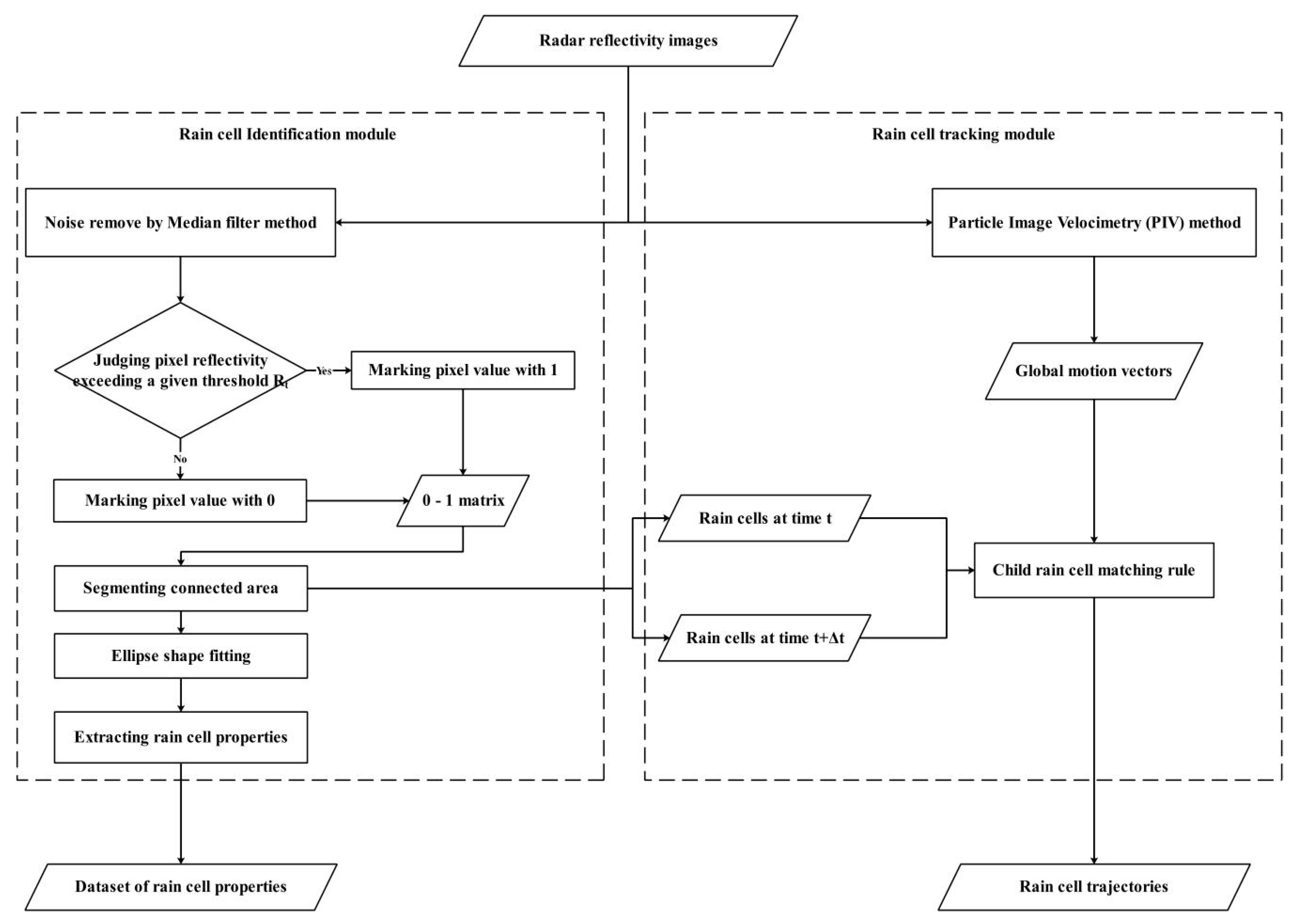
2. Methodology
2.1. Rain Cell Identification Module
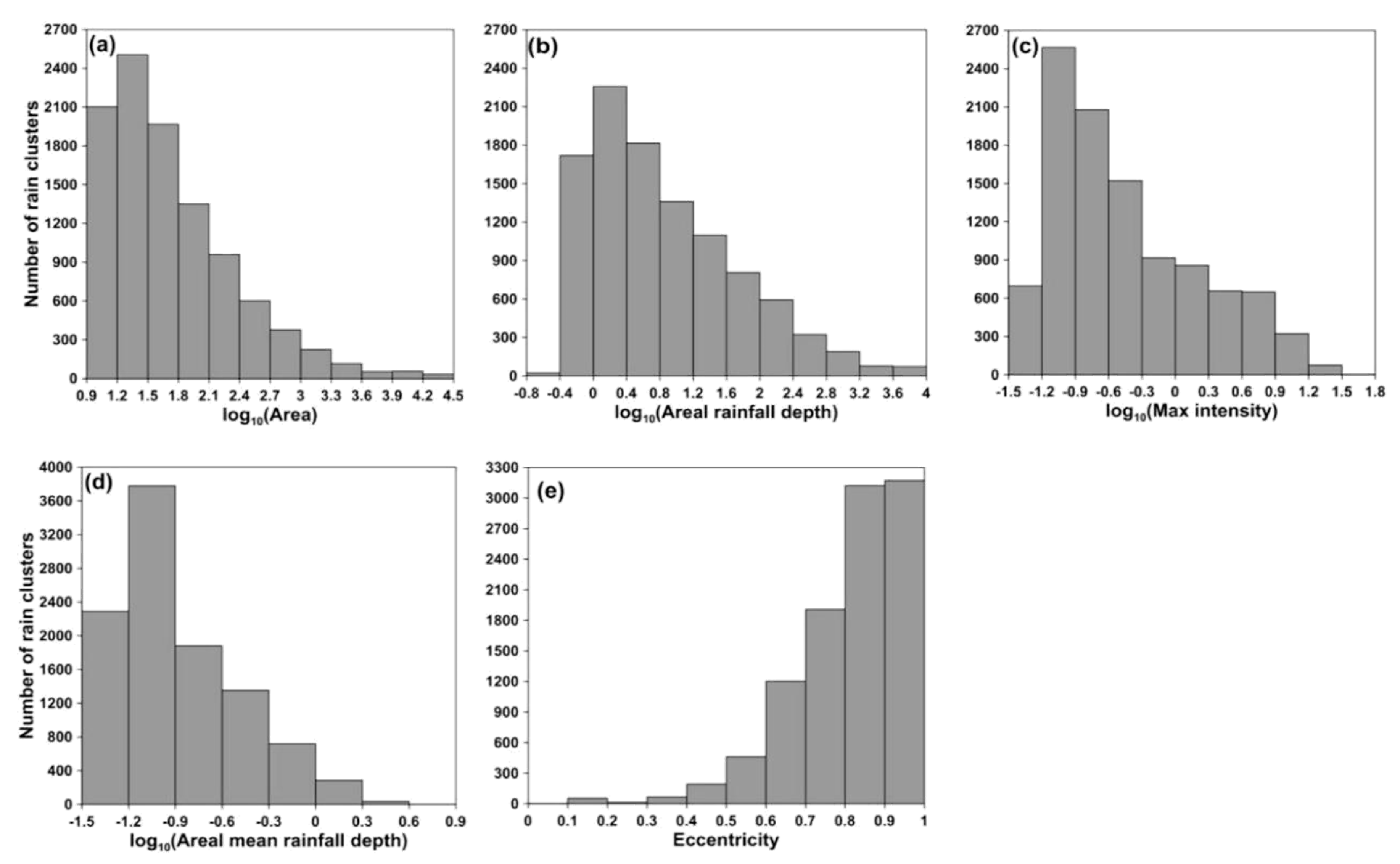
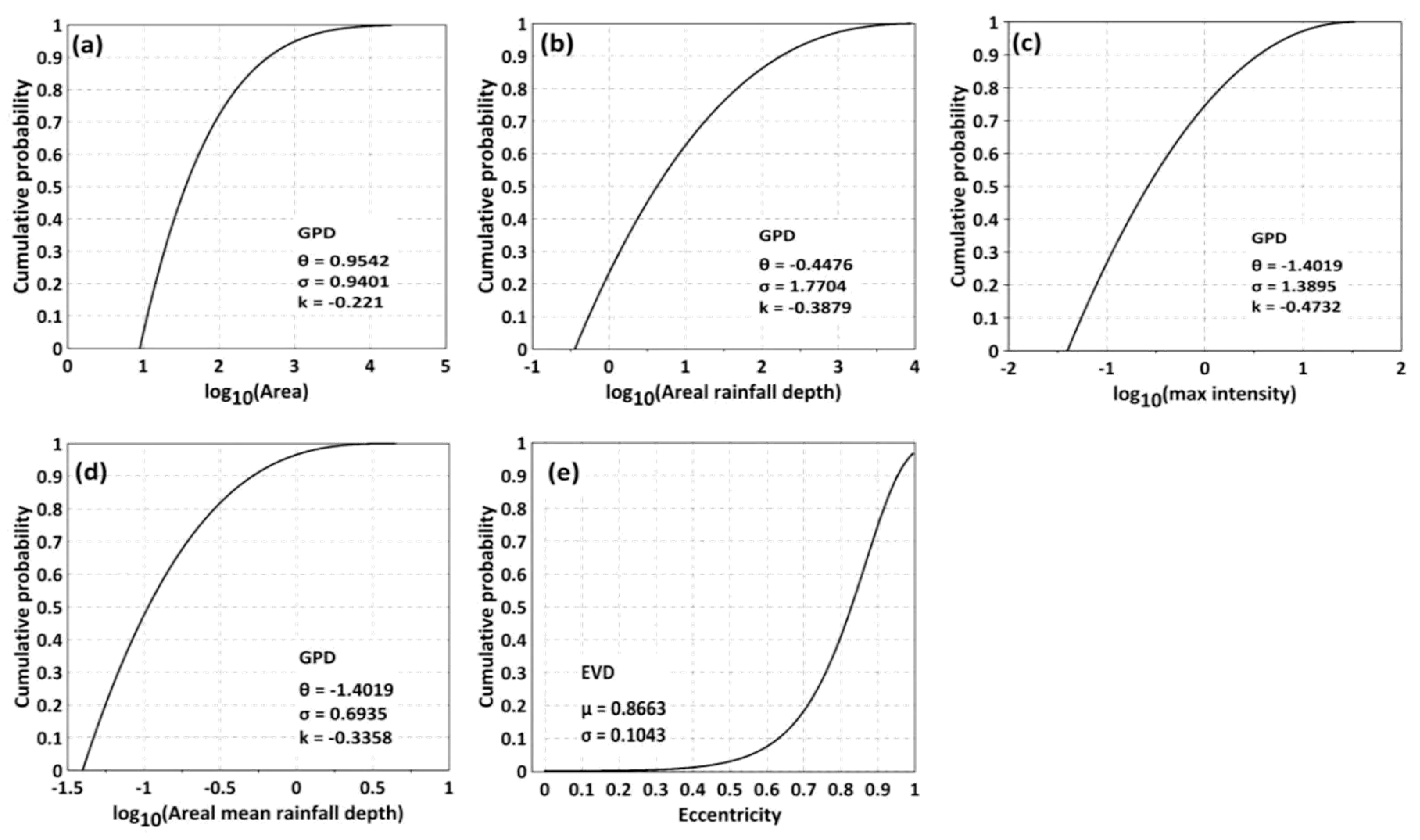
- Area (km2)—sum value for the number of pixels contained in one rain cell.
- Areal rainfall depth (mm)—cumulative precipitation of one rain cell over a 5-min interval.
- Maximum intensity (mm·h−1)—peak intensity of one rain cell.
- Areal mean rainfall depth (mm·km−2)—ratio of the areal rainfall depth and area.
- Eccentricity—ratio of minor and major axes, which are acquired from the fitted eclipse. Used to describe the shape of one rain cell with a value range from 0 to 1.
- Center of mass (km)—center of mass of a rain cell, which is weighted by the reflectivity of rainy pixels.
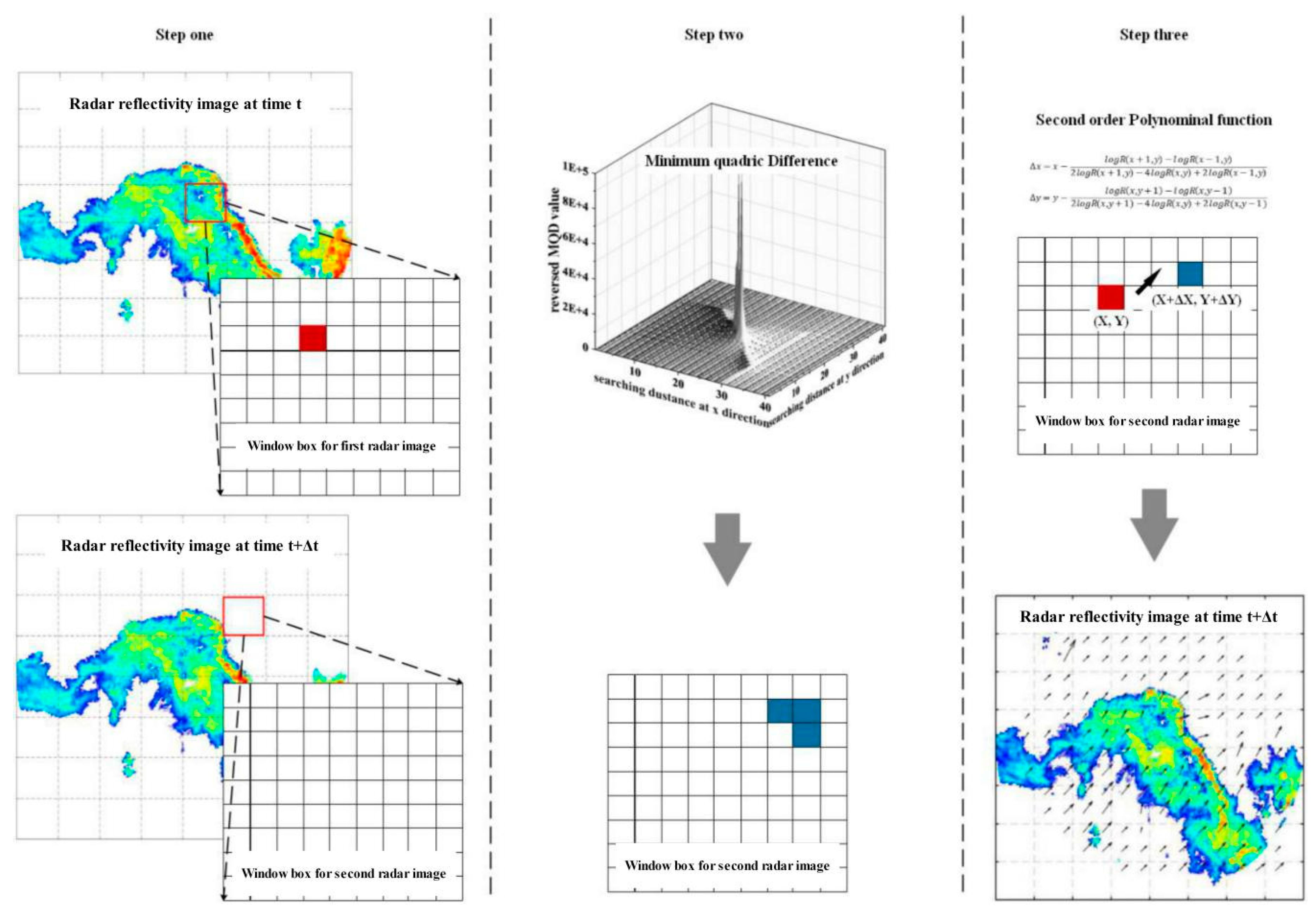
2.2. Rain Cell Tracking Module
- A boundary box of a parent cell is defined, with a horizontal length of (10 + max(posx), min(posx) − 10) and vertical length of (10 + max(posy), min(posy) − 10), where posx and posy are Cartesian coordinates of pixels in the parent cell.
- The number of child cells falling into the boundary box is determined and their properties, e.g., area, areal rainfall depth, max intensity, areal mean rainfall depth, and center of mass, are selected.
- If only one child cell is searched in the boundary box and it overlaps with a parent cell, then it is the most-matched rain cell. If this child cell does not overlap with a parent cell and the distance and angle difference for the center of mass between it and the parent cell are less than 3 × mean (Vmotion_vector) and 3 × θmotion_vector, it is also the most-matched rain cell, where mean (Vmotion_vector) and θmotion_vector are the mean value of velocity and the prevailing direction of the motion vector, respectively.
- If two or more child cells fall into the boundary box without overlapping a parent cell, the matching rule is changeless; however, one extra condition is included, i.e., child cells whose areas have minimum absolute differences with the parent cell are the most-matched rain cells.
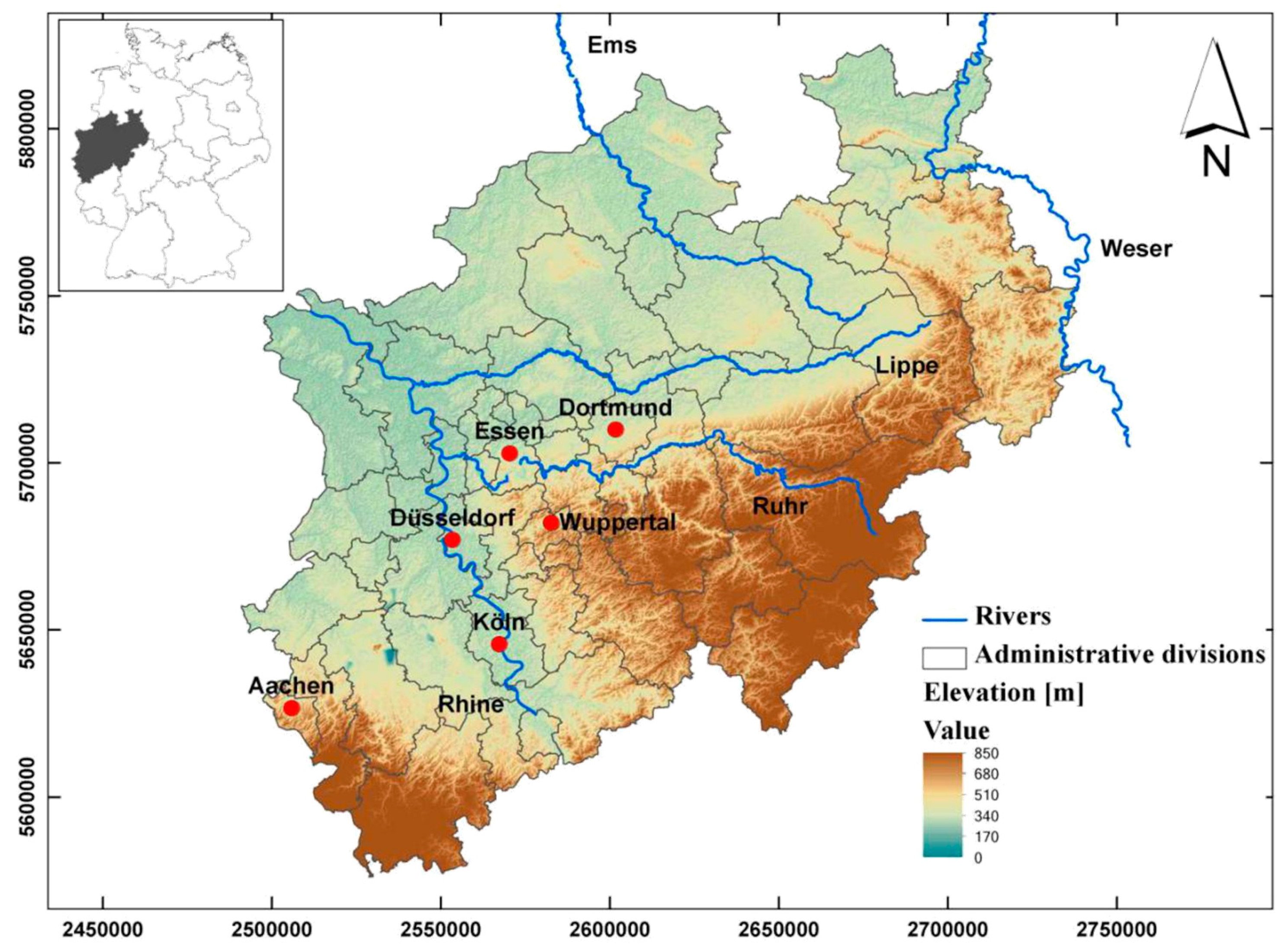
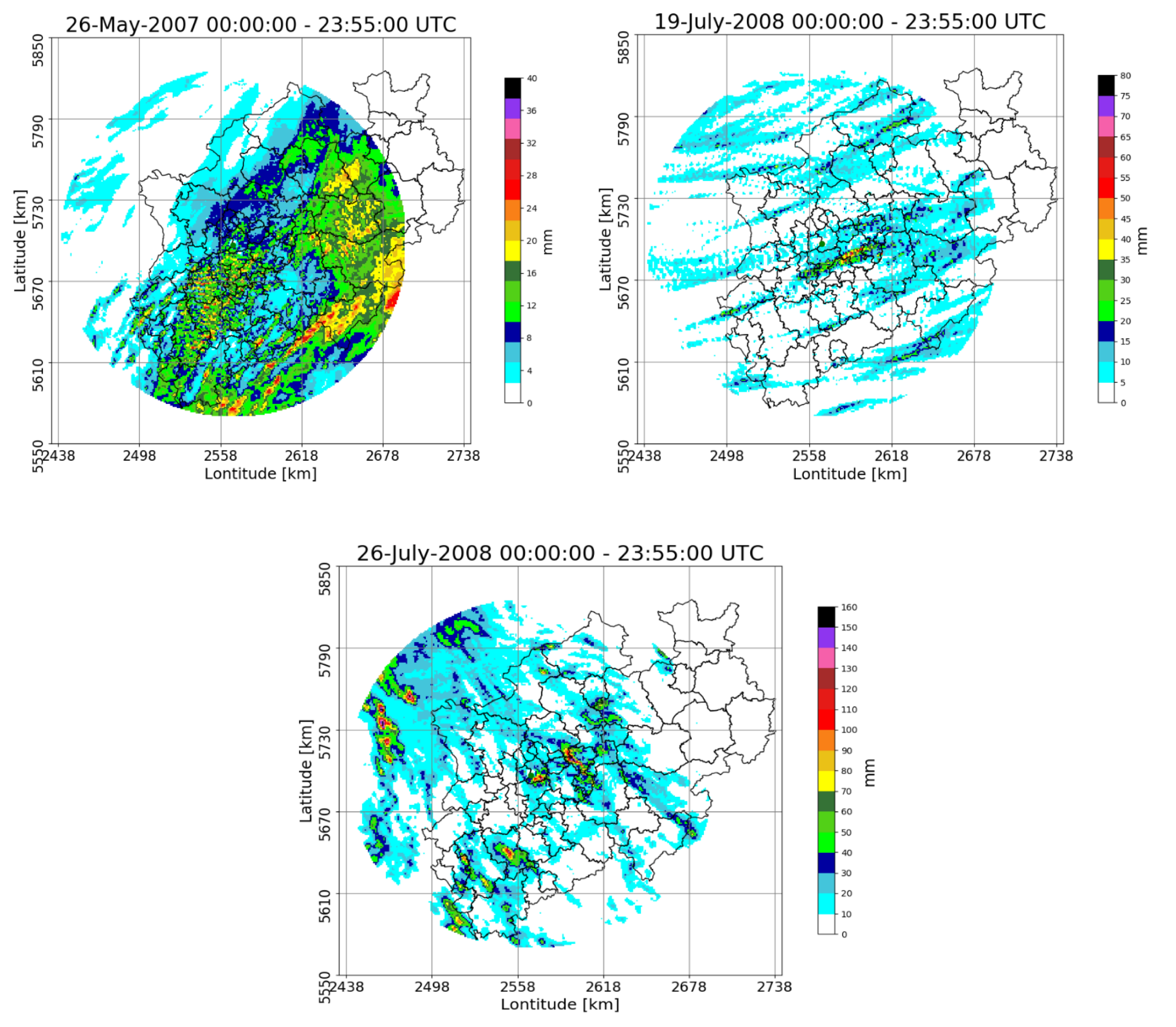
3. Study Area and Data
4. Results
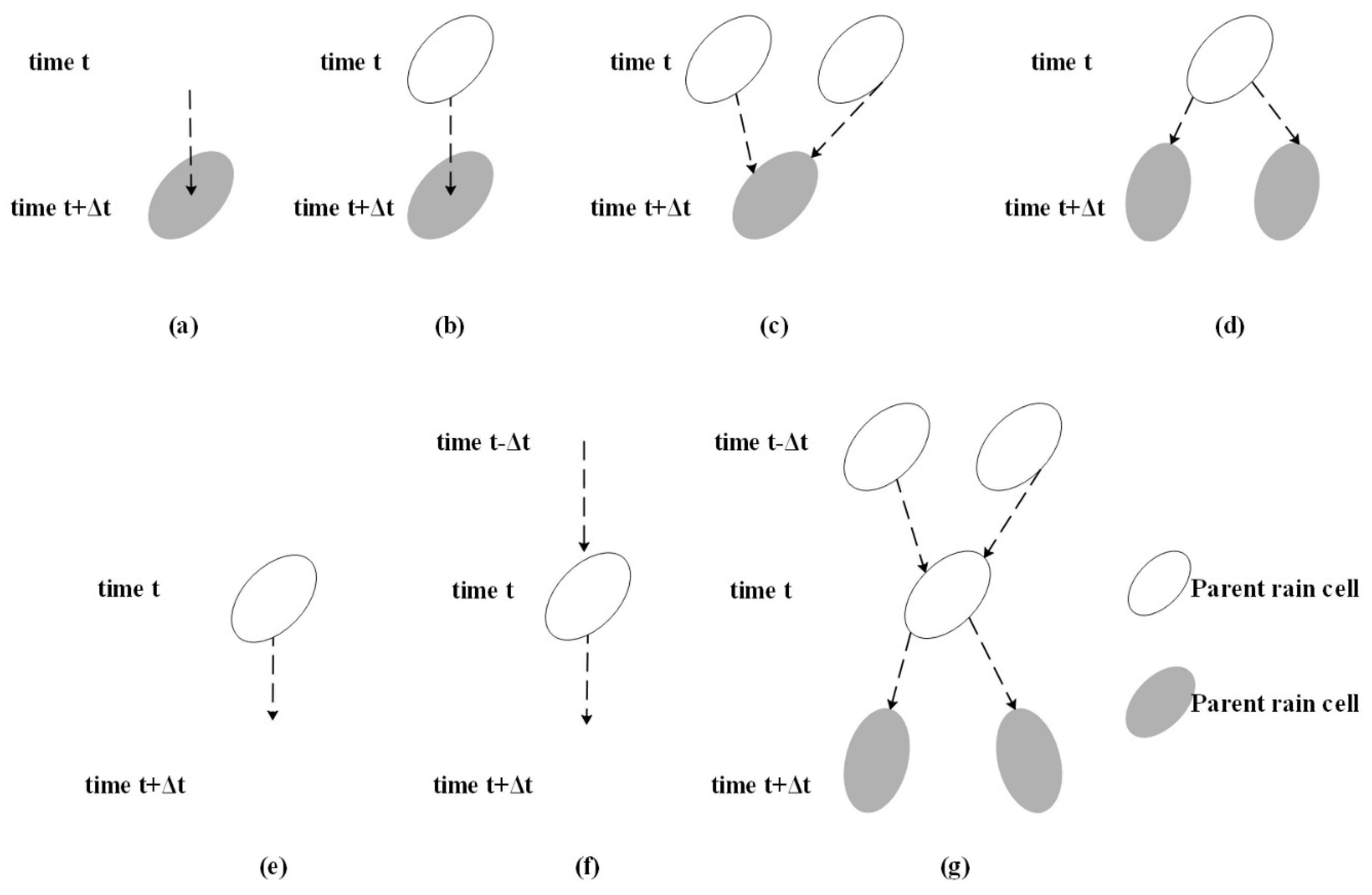
- Initial: A rain cell having no parent cell is termed an initial rain cell.
- Tracking: A rain cell with only one parent cell and having no interaction with other rain cells during its life cycle is termed a tracking rain cell.
- Merge: A rain cell with at least two parent cells is termed a merged rain cell.
- Split: A rain cell with only one parent cell but at least two child cells is termed a split rain cell.
- Dissipate: A rain cell with at least one parent cell but no child cells is termed a dissipate rain cell.
5. Discussion
5.1. Evaluation of Rain Cell Identification Module by Feature-Based Verification Methods
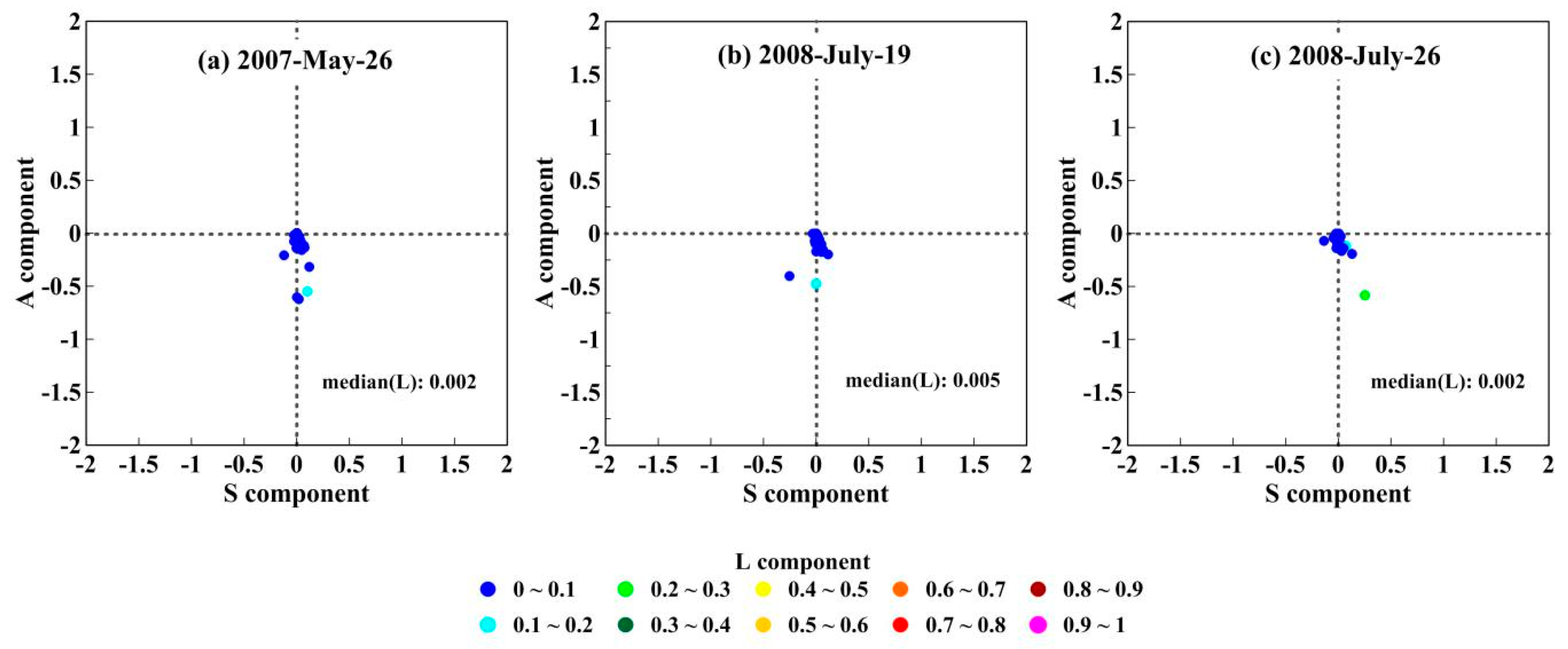
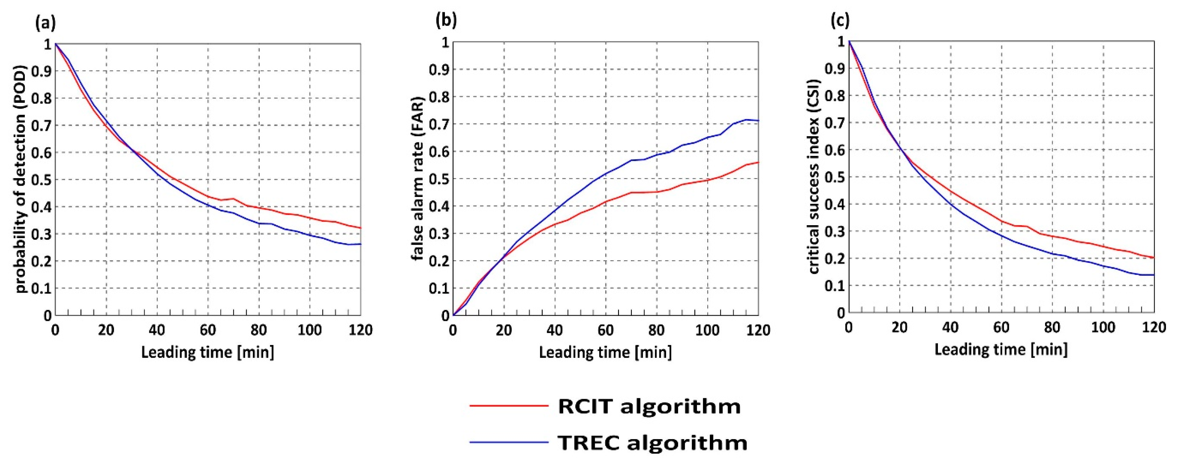
5.2. Assessing the Performance of Motion Estimation against the TREC Algorithm
5.3. Rain Cell Merging and Splitting Evaluation against the SCOUT Algorithm
6. Conclusions
- It uses the PIV method in rain cell motion estimation. Rain cell motion estimation by past algorithms is mainly based on the maximum correlation coefficient method, which may lead to nonconsecutive motion when the shape and volume of a rain cell change rapidly. The PIV method avoids this situation.
- A rain cell matching rule is proposed to discern the life cycle and stage change of rain cells. Some other algorithms focus mainly on analyzing feature changes of rain cells (e.g., overlap, area, intensity) by some object methods in dealing with cell merge and splits. The proposed rain cell matching rule put global motion vector as one judging parameter in rain cell stage analysis, this can be easily operated, and various stages of rain cells can also be discerned effectively.
Author Contributions
Funding
Acknowledgments
Conflicts of Interest
Appendix A
- The K–S test is based on the empirical cumulative distribution function (ECDF). Given N ordered data points Y1, Y2, …., Yn, their ECDF is defined as:where n(i) is the number of points less than Yi and Yj, which are ordered from the smallest to largest value. This is a step function that increases by 1/N at the value of each ordered data point. The K–S test was developed according to the following hypotheses: H0—the data follow a specified distribution; H1—the data do not follow the specified distribution.
- AIC [41] is based on the use of Kullback–Leible information as the discrepancy measure between the true distribution and the approximating distributions: Mi = gi(x, p1, p2, …, pn). The AIC for the ith candidate distribution can be computed as:where stands for the maximum log-likelihood of the sample of the data set, p is the parameter’s number of candidate distributions when the sample size n is small with respect to the number of the estimated parameter Pi. The smaller the value of AIC, the better fitting the result for the candidate distribution is.
- BIC [42] serves as an asymptotic approximation to a transformation of the Bayesian posterior probability of a candidate model. It is based on the empirical log-likelihood and does not require the specification of priors. BIC is defined as:where the symbols are the same as those in Equation (A2). A small value of BIC means that the candidate distribution fits well with the empirical distribution.
Appendix B
- Connectivity index: This is defined to compare simulated rain cells with respect to a reference object (e.g., observed rain cells). Its value is calculated based on the number of rain cells (NC) and the total number of non-zero pixels or pixels above a given threshold (NP), as in Equation (A4).where Cindex is the connectivity index, NP is the number of rainy pixels above a given threshold, and NC is the number of rain cells.
- Shape index: This index is introduced to quantitatively describe the shape discrepancy of rain cells, as in Equation (A5).where Sindex is the single index, Pmin is the theoretical minimum perimeter, and P is the actual perimeter of the rain cell.
- Area index: This is defined to depict the dispersiveness between the modeled and observed rain cells. Its value is the ratio of the area of its convex hull (the boundary of the minimal convex set containing a finite set of points in the rain cell), as in Equation (A6).where Aindex is the area of the rain cell and AConvex is the area of the convex hull.
References
- Cristiano, E.; Veldhuis, M.C.T.; Giesen, N.V.D. Spatial and temporal variability of rainfall and their effects on hydrological response in urban areas—A review. Hydrol. Earth Syst. Sci. 2017, 21, 1–34. [Google Scholar] [CrossRef]
- Peleg, N.; Blumensaat, F.; Molnar, P.; Fatichi, S.; Burlando, P. Partitioning the impacts of spatial and climatological rainfall variability in urban drainage modeling. Hydrol. Earth Syst. Sci. 2017, 21, 1–20. [Google Scholar] [CrossRef]
- Moseley, C.; Berg, P.; Haerter, J.O. Probing the precipitation life cycle by iterative rain cell tracking. J. Geophys. Res. Atmos. 2013, 118, 13361–13370. [Google Scholar] [CrossRef]
- Novo, S.; Martínez, D.; Puentes, O. Tracking, analysis, and nowcasting of Cuban convective cells as seen by radar. Meteorol. Appl. 2014, 21, 585–595. [Google Scholar] [CrossRef]
- Guinard, K.; Mailhot, A.; Caya, D. Projected changes in characteristics of precipitation spatial structures over North America. Int. J. Climatol. 2015, 35, 596–612. [Google Scholar] [CrossRef]
- Yeung, J.K.; Smith, J.A.; Baeck, M.L.; Villarini, G. Lagrangian Analyses of Rainfall Structure and Evolution for Organized Thunderstorm Systems in the Urban Corridor of the Northeastern US. J. Hydrometeorol. 2015, 16, 1575–1595. [Google Scholar] [CrossRef]
- Moral, A.D.; Rigo, T.; Llasat, M.C. A radar-based centroid tracking algorithm for severe weather surveillance: Identifying split/merge processes in convective systems. Atmos. Res. 2018, 213, 110–120. [Google Scholar] [CrossRef]
- Féral, L.; Sauvageot, H.; Castanet, L.; Lemorton, J.; Cornet, F.; Leconte, K. Large-scale modeling of rain fields from a rain cell deterministic model. Radio Sci. 2006, 41, 1–21. [Google Scholar] [CrossRef]
- Rinehart, R.E.; Garvey, E.T. Three-dimensional storm motion detection by conventional weather radar. Nature 1978, 273, 287–289. [Google Scholar] [CrossRef]
- Dixon, M.; Wiener, G. TITAN: Thunderstorm Identification, Tracking, Analysis, and Nowcasting—A Radar-based Methodology. J. Atmos. Ocean. Technol. 1993, 10, 785–797. [Google Scholar] [CrossRef]
- Li, L.; Schmid, W.; Joss, J. Nowcasting of Motion and Growth of Precipitation with Radar over a Complex Orography. J. Appl. Meteorol. 1995, 34, 1286–1300. [Google Scholar] [CrossRef]
- Li, P.W.; Lai, E.S.T. Applications of radar-based nowcasting techniques for mesoscale weather forecasting in Hong Kong. Meteorol. Appl. 2004, 11, 253–264. [Google Scholar] [CrossRef]
- Einfalt, T.; Denoeux, T.; Jacquet, G. A radar rainfall forecasting method designed for hydrological purposes. J. Hydrol. 1990, 114, 229–244. [Google Scholar] [CrossRef]
- Johnson, J.T.; Mackeen, P.L.; Witt, A.; Mitchell, E.D.W.; Stumpf, G.J.; Eilts, M.D.; Thomas, K.W. The Storm Cell Identification and Tracking Algorithm: An Enhanced WSR-88D Algorithm. Weather Forecast. 1998, 13, 263–276. [Google Scholar] [CrossRef]
- Handwerker, J. Cell tracking with TRACE3D—A new algorithm. Atmos. Res. 2002, 61, 15–34. [Google Scholar] [CrossRef]
- Zahraei, A.; Hsu, K.L.; Sorooshian, S.; Gourley, J.J.; Hong, Y.; Behrangi, A. Short-term quantitative precipitation forecasting using an object-based approach. J. Hydrol. 2013, 483, 1–15. [Google Scholar] [CrossRef]
- Munoz, C.; Wang, L.P.; Willems, P. Enhanced object-based tracking algorithm for convective rain storms and cells. Atmos. Res. 2017, 201, 144–158. [Google Scholar] [CrossRef]
- Jung, S.H.; Lee, G. Radar-based cell tracking with fuzzy logic approach. Meteorol. Appl. 2015, 22, 716–730. [Google Scholar] [CrossRef]
- Shah, S.; Notarpietro, R.; Branca, M. Storm Identification, Tracking and Forecasting Using High-Resolution Images of Short-Range X-Band Radar. Atmosphere 2015, 6, 579–606. [Google Scholar] [CrossRef]
- Hou, J.; Wang, P. Storm Tracking via Tree Structure Representation of Radar Data. J. Atmos. Ocean. Technol. 2017, 34, 729–747. [Google Scholar] [CrossRef]
- Zan, B.; Yu, Y.; Li, J.; Zhao, G.; Zhang, T.; Ge, J. Solving the storm split-merge problem—A combined storm identification, tracking algorithm. Atmos. Res. 2019, 218, 335–346. [Google Scholar] [CrossRef]
- Anoraganingrum, D. Cell Segmentation with Median Filter and Mathematical Morphology Operation. In Proceedings of the 10th International Conference on Image Analysis and Processing, Venice, Italy, 27–29 September 1999; p. 1043. [Google Scholar]
- Peleg, N.; Morin, E. Convective rain cells: Radar-derived spatiotemporal characteristics and synoptic patterns over the eastern Mediterranean. J. Geophys. Res. Atmos. 2012, 117. [Google Scholar] [CrossRef]
- Merzkirch, W. Particle Image Velocimetry. In Optical Measurements: Techniques and Applications; Mayinger, F., Feldmann, O., Eds.; Springer: Berlin/Heidelberg, Germany, 2001; pp. 341–357. [Google Scholar]
- Adrian, R.J. Twenty years of particle image velocimetry. Exp. Fluids 2005, 39, 159–169. [Google Scholar] [CrossRef]
- Westerweel, J.; Elsinga, G.E.; Adrian, R.J. Particle Image Velocimetry for Complex and Turbulent Flows. Annu. Rev. Fluid Mech. 2013, 45, 409. [Google Scholar] [CrossRef]
- Gui, L.C.; Merzkirch, W. A method of tracking ensembles of particle images. Exp. Fluids 1996, 21, 465–468. [Google Scholar] [CrossRef]
- Golz, C.; Einfalt, T.; Galli, G. Radar data quality control methods in VOLTAIRE. Meteorol. Z. 2006, 15, 497–504. [Google Scholar] [CrossRef]
- Heistermann, M.; Jacobi, S.; Pfaff, T. Technical Note: An open source library for processing weather radar data (wradlib). Hydrol. Earth Syst. Sci. 2013, 17, 863–871. [Google Scholar] [CrossRef]
- Weusthoff, T.; Hauf, T. The life cycle of convective-shower cells under post-frontal conditions. Q. J. R. Meteorol. Soc. 2010, 134, 841–857. [Google Scholar] [CrossRef]
- Frerk, I.; Treis, A.; Einfalt, T.; Jessen, M. Ten years of quality controlled and adjusted radar precipitation data for north rhine-westphalia–methods and objectives. In Proceedings of the 9th International Workshop on Precipitation in Urban Areas: Urban Challenges in Rainfall Analysis, Pontresina, Switzerland, 2012. [Google Scholar]
- Barnolas, M.; Rigo, T.; Llasat, M.C. Characteristics of 2-D convective structures in Catalonia (NE Spain): An analysis using radar data and GIS. Hydrol. Earth Syst. Sci. 2010, 14, 129–139. [Google Scholar] [CrossRef]
- Byers, H.R.; Braham, R.R. Thunderstorm structure and circulation. J. Meteorol. 1948, 5, 71–86. [Google Scholar] [CrossRef]
- Zhao, B.; Zhang, B. Assessing Hourly Precipitation Forecast Skill with the Fractions Skill Score. J. Meteorol. Res. 2018, 32, 135–145. [Google Scholar] [CrossRef]
- Davis, C.; Brown, B.; Bullock, R. Object-Based Verification of Precipitation Forecasts. Part I: Methodology and Application to Mesoscale Rain Areas. Mon. Weather Rev. 2006, 134, 1772–1784. [Google Scholar] [CrossRef]
- Gilleland, E.; Ahijevych, D.; Brown, B.G.; Casati, B.; Ebert, E.E. Intercomparison of Spatial Forecast Verification Methods. Weather Forecast. 2009, 24, 1416–1430. [Google Scholar] [CrossRef]
- Ebert, B.; Fowler, T.; Gill, P.; Goeber, M.; Joslyn, S.; Mittermaier, M.; Nurmi, P.; Watkins, A.; Weigel, A. Progress and challenges in forecast verification. Meteorol. Appl. 2013, 20, 129. [Google Scholar] [CrossRef]
- Wernli, H.; Paulat, M.; Hagen, M.; Frei, C. SAL—A Novel Quality Measure for the Verification of Quantitative Precipitation Forecasts. Mon. Weather Rev. 2008, 136, 4470–4487. [Google Scholar] [CrossRef]
- Aghakouchak, A.; Nasrollahi, N.; Li, J.; Imam, B.; Sorooshian, S. Geometrical Characterization of Precipitation Patterns. J. Polym. Environ. 2011, 19, 818. [Google Scholar] [CrossRef]
- Germann, U.; Zawadzki, I.; Turner, B. Predictability of Precipitation from Continental Radar Images. Part IV: Limits to Prediction. J. Atmos. Sci. 2006, 63, 2092–2108. [Google Scholar] [CrossRef]
- Akaike, H. Information Theory and an Extension of the Maximum Likelihood Principle. In Selected Papers of Hirotugu Akaike; Parzen, E., Tanabe, K., Kitagawa, G., Eds.; Springer: New York, NY, USA, 1998; pp. 199–213. [Google Scholar]
- Schwarz, G. Estimating the Dimension of a Model. Annal. Stat. 2005, 6, 15–18. [Google Scholar] [CrossRef]


| Z (dBZ) | R (mm·h−1) | Rain Rate (mm·5 min−1) |
|---|---|---|
| >55 | >150 | >12.5 |
| 46–55 | 35–150 | 2.92–12.5 |
| 37–46 | 8.1–35 | 0.68–2.92 |
| 28–37 | 1.9–8.1 | 0.16–0.68 |
| 19–28 | 0.4–1.9 | 0.03–0.16 |
| 7–19 | 0.06–0.4 | 0.005–0.03 |
| Property | Statistical Properties | |||
|---|---|---|---|---|
| Minimum Value | Maximum Value | Standard Deviation | Median | |
| Area (km2) | 9 | 18,734 | 1391 | 38 |
| Areal rainfall depth (mm) | 0.36 | 8861 | 559.9 | 4.4 |
| Max intensity (mm·h−1) | 0.48 | 397.75 | 34.08 | 2.83 |
| Areal mean rainfall depth (mm·km−2) | 0.04 | 4.4 | 0.3 | 0.1 |
| Eccentricity | 0 | 0.99 | 0.17 | 0.84 |
| Stages | 26 May 2007 | 19 July 2008 | 26 July 2008 |
|---|---|---|---|
| Initial | 158 | 350 | 471 |
| Tracking | 608 | 1270 | 1787 |
| Merge | 7 | 6 | 39 |
| Split | 1 | 2 | 5 |
| Dissipate | 152 | 346 | 434 |
| 5-min life cycle | 632 | 3148 | 929 |
| Complex stage | 0 | 0 | 1 |
| Selected Cases | Connectivity Index | Shape Index | Area Index | |||||||
|---|---|---|---|---|---|---|---|---|---|---|
| 25% | 50% | 75% | 25% | 50% | 75% | 25% | 50% | 75% | ||
| 26 May 2007 | obs | 0.934 | 0.957 | 0.977 | 0.22 | 0.325 | 0.509 | 0.102 | 0.198 | 0.417 |
| sim | 0.966 | 0.979 | 0.992 | 0.27 | 0.378 | 0.579 | 0.135 | 0.271 | 0.53 | |
| 19 July 2008 | obs | 0.847 | 0.895 | 0.938 | 0.143 | 0.217 | 0.29 | 0.031 | 0.071 | 0.118 |
| sim | 0.907 | 0.943 | 0.969 | 0.154 | 0.233 | 0.297 | 0.043 | 0.086 | 0.134 | |
| 26 July 2008 | obs | 0.897 | 0.93 | 0.955 | 0.154 | 0.245 | 0.374 | 0.045 | 0.116 | 0.213 |
| sim | 0.936 | 0.965 | 0.997 | 0.189 | 0.285 | 0.385 | 0.077 | 0.149 | 0.238 | |
| Date | Duration | Max. Total Rainfall (mm) | Max. Intensity (mm·5 min−1) |
|---|---|---|---|
| 26 May 2007 | 00:00~02:10 | 25.8 | 22.1 |
| 26 May 2007 | 19:00~21:10 | 39.5 | 36 |
| 19 July 2008 | 02:00~04:10 | 15.6 | 7.7 |
| 19 July 2008 | 13:00~15:10 | 34.7 | 33.2 |
| 19 July 2008 | 16:00~18:10 | 81.3 | 53.9 |
| 26 July 2008 | 00:00~02:10 | 133.3 | 36 |
| 26 July 2008 | 13:00~15:10 | 177.4 | 49.7 |
| 26 July 2008 | 16:00~18:10 | 144 | 58.5 |
| POD | FAR | CSI | ||||
|---|---|---|---|---|---|---|
| RCIT | SCOUT | RCIT | SCOUT | RCIT | SCOUT | |
| Initial | 0.98 | 0.87 | 0.11 | 0.07 | 0.88 | 0.81 |
| Tracking | 0.98 | 0.97 | 0.002 | 0.001 | 0.98 | 0.97 |
| Merge | 0.83 | 0.75 | 0.17 | 0.4 | 0.71 | 0.5 |
| Split | 0.8 | 0.67 | 0 | 0.33 | 0.8 | 0.5 |
| Dissipation | 0.98 | 0.99 | 0.02 | 0.004 | 0.96 | 0.99 |
© 2019 by the authors. Licensee MDPI, Basel, Switzerland. This article is an open access article distributed under the terms and conditions of the Creative Commons Attribution (CC BY) license (http://creativecommons.org/licenses/by/4.0/).
Share and Cite
He, T.; Einfalt, T.; Zhang, J.; Hua, J.; Cai, Y. New Algorithm for Rain Cell Identification and Tracking in Rainfall Event Analysis. Atmosphere 2019, 10, 532. https://doi.org/10.3390/atmos10090532
He T, Einfalt T, Zhang J, Hua J, Cai Y. New Algorithm for Rain Cell Identification and Tracking in Rainfall Event Analysis. Atmosphere. 2019; 10(9):532. https://doi.org/10.3390/atmos10090532
Chicago/Turabian StyleHe, Ting, Thomas Einfalt, Jianxin Zhang, Jiyao Hua, and Yang Cai. 2019. "New Algorithm for Rain Cell Identification and Tracking in Rainfall Event Analysis" Atmosphere 10, no. 9: 532. https://doi.org/10.3390/atmos10090532
APA StyleHe, T., Einfalt, T., Zhang, J., Hua, J., & Cai, Y. (2019). New Algorithm for Rain Cell Identification and Tracking in Rainfall Event Analysis. Atmosphere, 10(9), 532. https://doi.org/10.3390/atmos10090532