Deep Random Subspace Learning: A Spatial-Temporal Modeling Approach for Air Quality Prediction

Abstract
:1. Introduction
2. Method
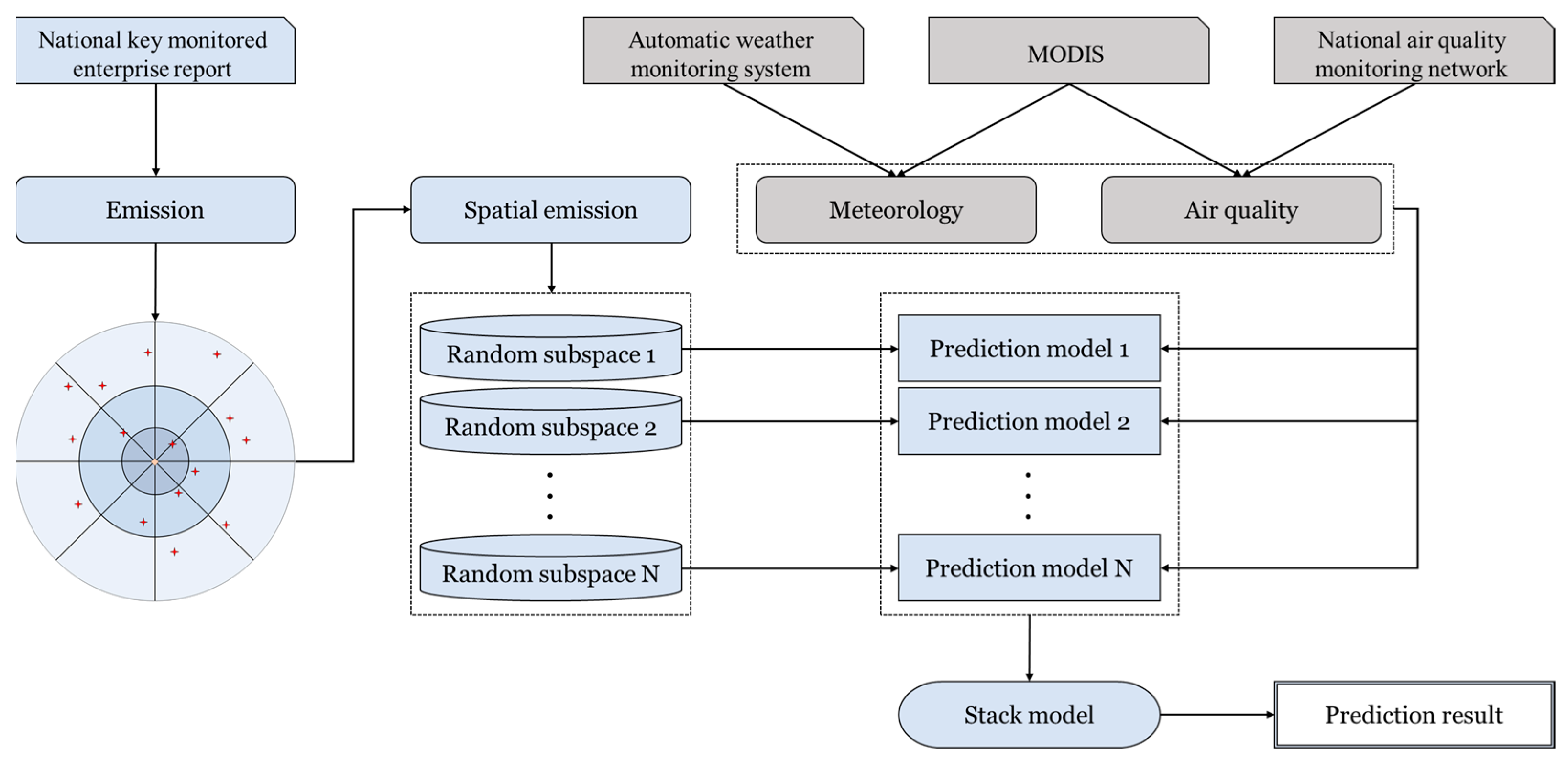
2.1. Overview
2.2. Data Collection and Preprocessing
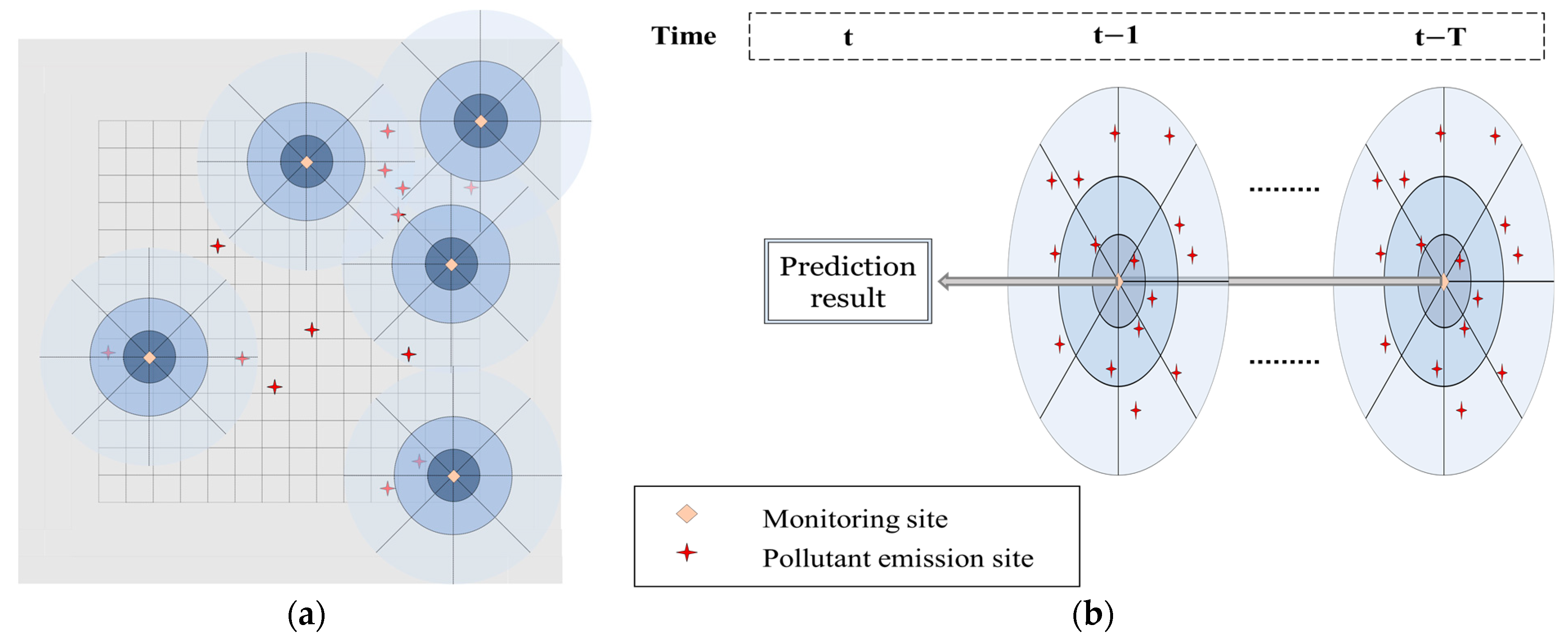
2.3. Emission Features Based on Spatial-Temporal Analysis
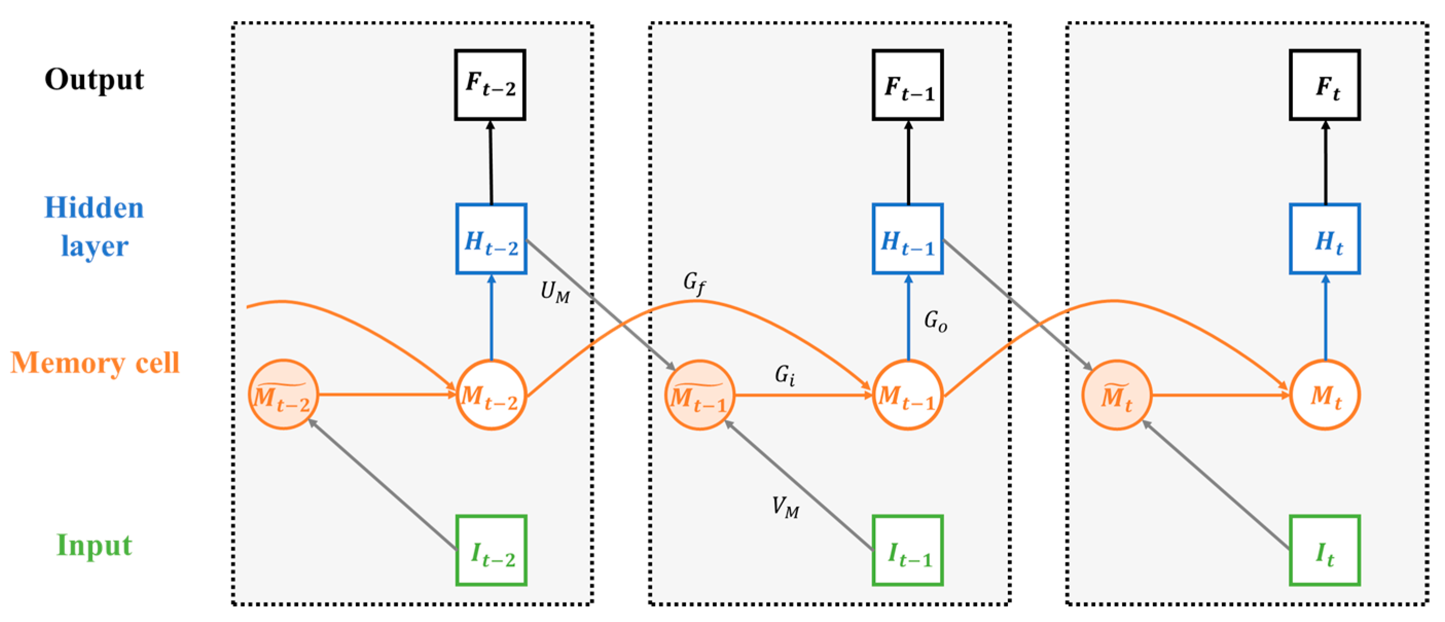
2.4. Modeling and Prediction
| Algorithm 1: Learning LSTM-DRSL through BPTT |
| Input: Training samples ; |
| Output: Weight matrices , , , , , , , and for base models respectively ( is the number of random subspaces); stack model ; |
| 1: Initialize , , , , , , , , and randomly; 2: Set prediction time window ; |
| 3: Sort input samples in chronological order from to ; |
| 4: Set time stamp ; 5: Initialize the serial number of random subspaces ; 6: // Build random subspaces 7: while do 8: Randomly sample of emission features and integrate them with other 9: features into ; 10: ; 11: end while 12: ; 13: // Training the base LSTM models and the stack model |
| 14: while not converge do |
| 15: while do |
| 16: while do |
| 17: Compute based on ; (Formula (1)~(7), (9)) |
| 18: Compute at ; (Formula (8)) |
| 19: Update weight matrices for model ; (BPTT) 20: Obtain prediction value ; 21: ; 22: end while 23: Train the stack model ; |
| 24: ; 25: end while |
| 26: end while |
3. Experiment
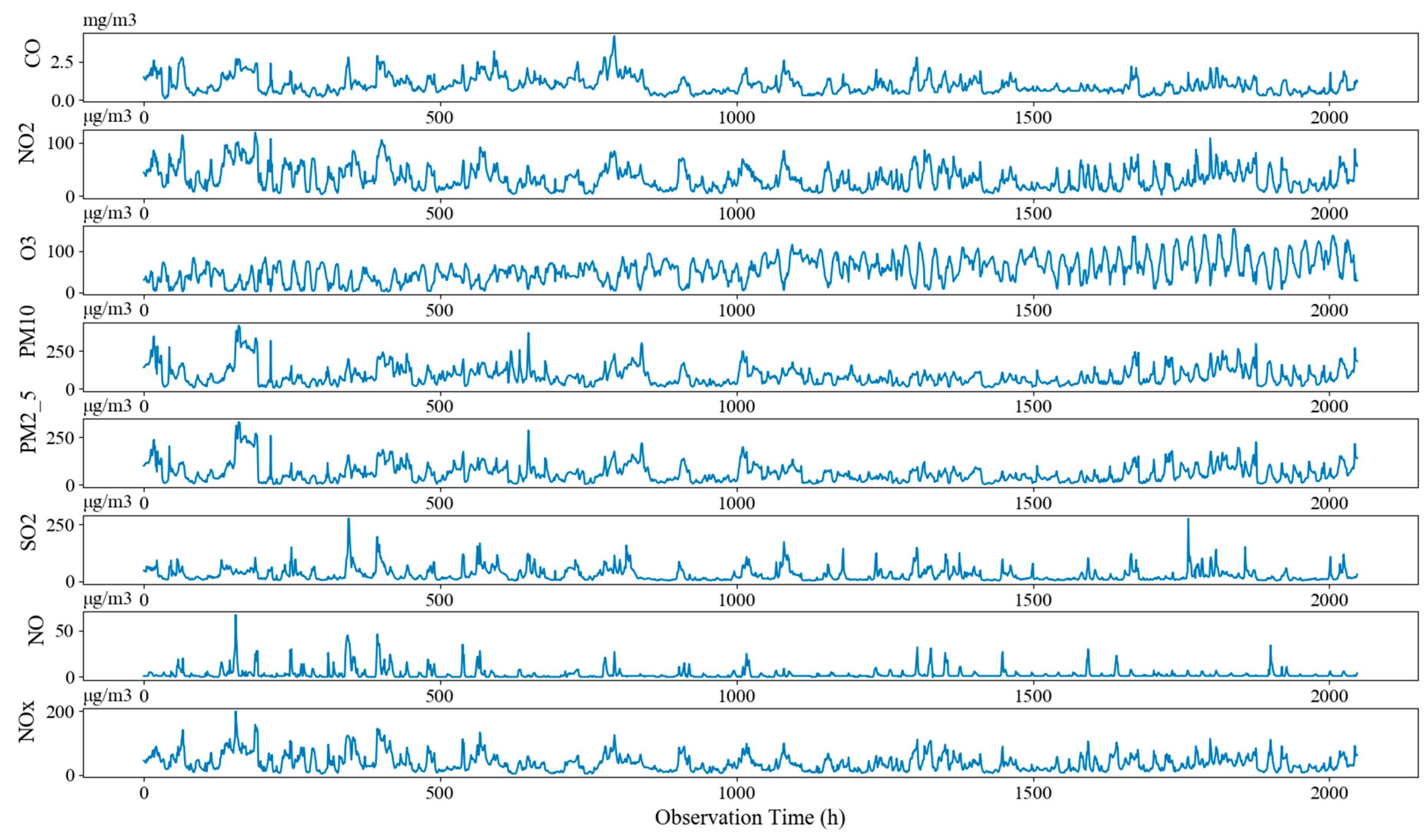
3.1. Data Description
3.2. Evaluation Metrics
3.3. Experiment Design
4. Results and Analysis
4.1. Comparison with Baseline Models
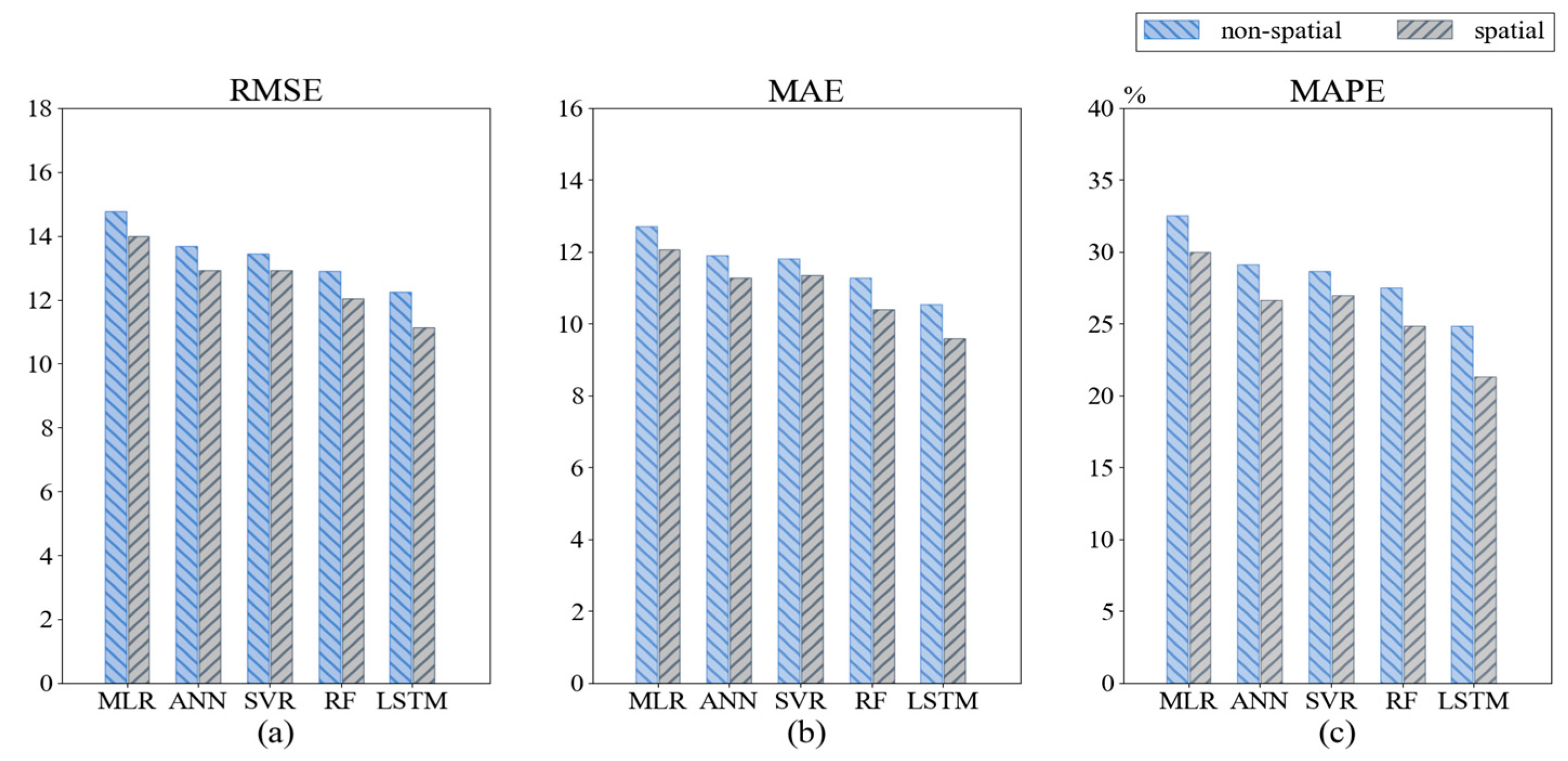
4.2. Incremental Effect of Combined Spatial Features
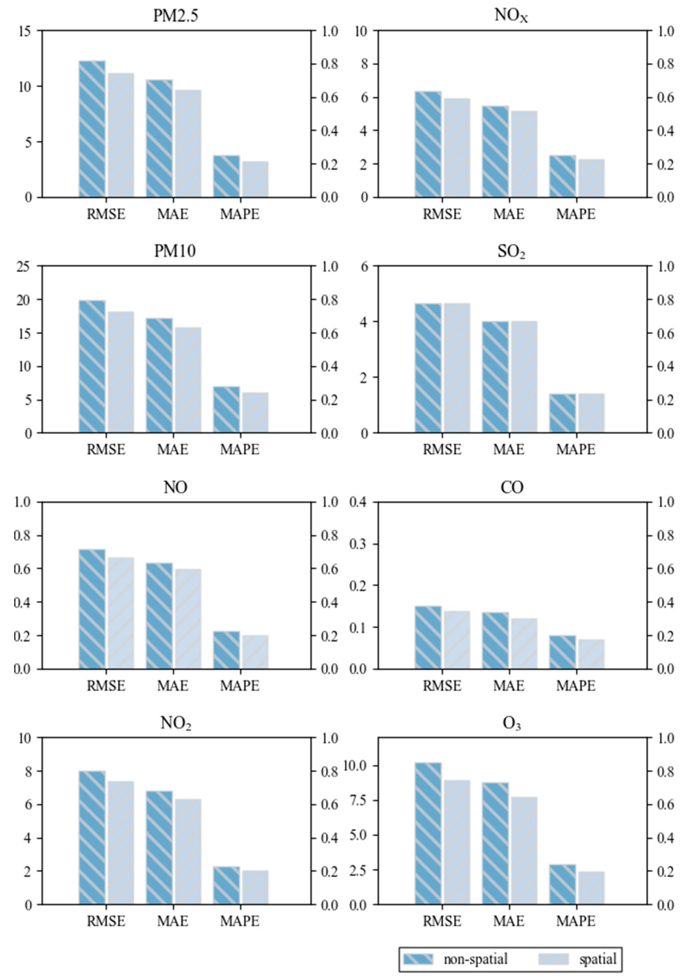
4.3. Overall Improvement with Random Subspace Ensemble
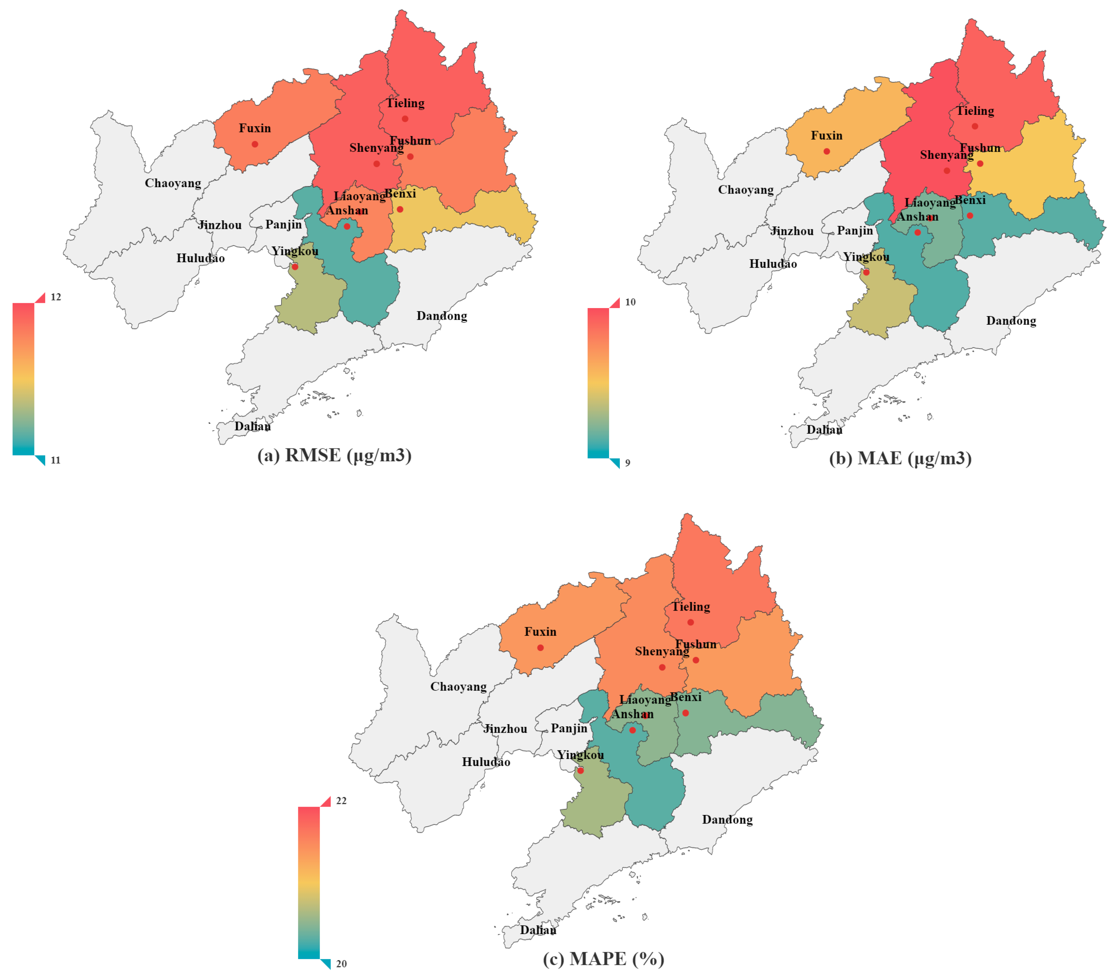
4.4. Performance Comparison with Consideration of Spatial Variations
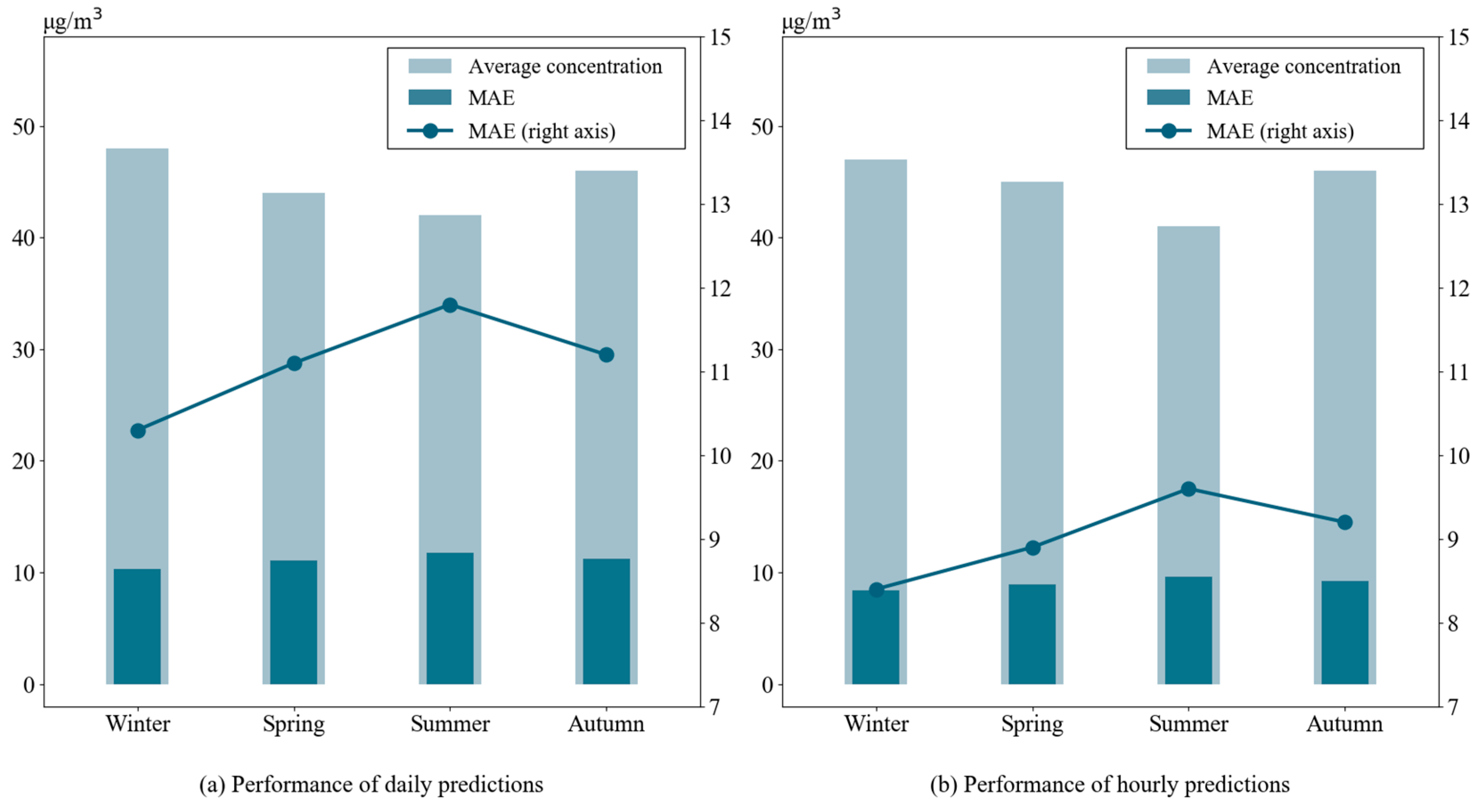
4.5. Performance Comparison with Consideration of Temporal Variations
5. Conclusions
Author Contributions
Funding
Acknowledgments
Conflicts of Interest
Appendix A
References
- Health Effects Institute, State of Global Air 2018. Available online: https://www.stateofglobalair.org/archives, 2018 (accessed on 21 March 2019).
- Kloog, I.; Ridgway, B.; Koutrakis, P.; Coull, B.A.; Schwartz, J.D. Long- and short-term exposure to PM2.5 and mortality: Using novel exposure models. Epidemiology 2013, 24, 555–561. [Google Scholar] [CrossRef] [PubMed]
- Ebenstein, A.; Fan, M.; Greenstone, M.; He, G.; Zhou, M. New evidence on the impact of sustained exposure to air pollution on life expectancy from china’s huai river policy. Proc. Natl. Acad. Sci. USA 2013, 110, 12936–12941. [Google Scholar] [CrossRef] [PubMed]
- Schwartz, J. Particulate air pollution and chronic respiratory disease. Environ. Res. 1993, 62, 7–13. [Google Scholar] [CrossRef]
- Chan, C.K.; Yao, X. Air pollution in mega cities in china. Atmos. Environ. 2008, 42, 1–42. [Google Scholar] [CrossRef]
- American Lung Association, State of the Air 2018. Available online: https://www.lung.org/assets/documents/healthy-air/state-of-the-air/sota-2018-full.pdf (accessed on 21 March 2019).
- Ferretti, V.; Montibeller, G. Key challenges and meta-choices in designing and applying multi-criteria spatial decision support systems. Decis. Support Syst. 2016, 84, 41–52. [Google Scholar] [CrossRef]
- Zhu, S.; Lian, X.; Liu, H.; Hu, J.; Wang, Y.; Che, J. Daily air quality index forecasting with hybrid models: A case in China. Environ. Pollut. 2017, 231, 1232–1244. [Google Scholar] [CrossRef] [PubMed]
- Xu, B.; Lin, H.; Chiu, L.; Hu, Y.; Zhu, J.; Hu, M.; Cui, W. Collaborative virtual geographic environments: A case study of air pollution simulation. Inform. Sci. 2011, 181, 2231–2246. [Google Scholar] [CrossRef]
- Werner, M.; Kryza, M.; Ojrzynska, H.; Skjoth, C.A.; Walaszek, K.; Dore, A.J. Application of WRF-Chem to forecasting PM10 concentration over Poland. Int. J. Environ. Pollut. 2015, 58, 280–292. [Google Scholar] [CrossRef]
- Beevers, S.D.; Nutthida, K.; Williams, M.L.; Carslaw, D.C. One way coupling of CMAQ and a road source dispersion model for fine scale air pollution predictions. Atmos. Environ. 2012, 59, 47–58. [Google Scholar] [CrossRef]
- Abdul-Wahab, S.; Sappurd, A.; Al-Damkhi, A. Application of California Puff (CALPUFF) model: A case study for Oman. Clean Technol. Environ. Policy 2011, 13, 177–189. [Google Scholar] [CrossRef]
- Tartakovsky, D.; Broday, D.M.; Stern, E. Evaluation of AERMOD and CALPUFF for predicting ambient concentrations of total suspended particulate matter (TSP) emissions from a quarry in complex terrain. Environ. Pollut. 2013, 179, 138–145. [Google Scholar] [CrossRef]
- Byun, D.; Schere, K.L. Review of the governing equations, computational algorithms, and other components of the Models-3 Community Multiscale Air Quality (CMAQ) modeling system. Appl. Mech. Rev. 2006, 59, 51–77. [Google Scholar] [CrossRef]
- Done, J.; Davis, C.A.; Weisman, M. The next generation of NWP: Explicit forecasts of convection using the Weather Research and Forecasting (WRF) model. Atmos. Sci. Lett. 2004, 5, 110–117. [Google Scholar] [CrossRef]
- Grell, G.A.; Peckham, S.E.; Schmitz, R.; McKeen, S.A.; Frost, G.; Skamarock, W.C.; Eder, B. Fully coupled “online” chemistry within the WRF model. Atmos. Environ. 2005, 39, 6957–6975. [Google Scholar] [CrossRef]
- Global Forecast Plots-Copernicus. Available online: https://atmosphere.copernicus.eu/global-forecast-plots (accessed on 20 July 2019).
- Taheri Shahraiyni, H.; Sodoudi, S. Statistical modeling approaches for PM10 prediction in urban areas; A review of 21st-century studies. Atmosphere 2016, 7, 15. [Google Scholar] [CrossRef]
- Wang, Y.; Xu, W. Leveraging deep learning with LDA-based text analytics to detect automobile insurance fraud. Decis. Support Syst. 2018, 105, 87–95. [Google Scholar] [CrossRef]
- Lv, M.; Li, Y.; Chen, L.; Chen, T. Air quality estimation by exploiting terrain features and multi-view transfer semi-supervised regression. Inform. Sci. 2019, 483, 82–95. [Google Scholar] [CrossRef]
- Bai, L.; Wang, J.; Ma, X.; Lu, H. Air pollution forecasts: An overview. Int. J. Environ. Res. Public Health 2018, 15, 780. [Google Scholar] [CrossRef]
- Yang, C.S.; Wei, C.P.; Yuan, C.C.; Schoung, J.Y. Predicting the length of hospital stay of burn patients: Comparisons of prediction accuracy among different clinical stages. Decis. Support Syst. 2010, 50, 325–335. [Google Scholar] [CrossRef]
- Yu, R.; Yang, Y.; Yang, L.; Han, G.; Move, O. RAQ—A random forest approach for predicting air quality in urban sensing systems. Sensors 2016, 16, 86. [Google Scholar] [CrossRef]
- Lin, K.P.; Pai, P.F.; Yang, S.L. Forecasting concentrations of air pollutants by logarithm support vector regression with immune algorithms. Appl. Math. Comput. 2011, 217, 5318–5327. [Google Scholar] [CrossRef]
- Wang, P.; Liu, Y.; Qin, Z.; Zhang, G. A novel hybrid forecasting model for PM10 and SO2 daily concentrations. Sci. Total Environ. 2015, 505, 1202–1212. [Google Scholar] [CrossRef] [PubMed]
- Wang, J.; Zhang, X.; Guo, Z.; Lu, H. Developing an early-warning system for air quality prediction and assessment of cities in China. Expert Syst. Appl. 2017, 84, 102–116. [Google Scholar] [CrossRef]
- Rahman, N.H.A.; Lee, M.H.; Latif, M.T. Artificial neural networks and fuzzy time series forecasting: An application to air quality. Qual. Quant. 2015, 49, 1–15. [Google Scholar] [CrossRef]
- Meissner, M.; Schmuker, M.; Schneider, G. Optimized Particle Swarm Optimization (OPSO) and its application to artificial neural network training. BMC Bioinform. 2006, 7, 125. [Google Scholar] [CrossRef]
- Huang, X.; Qi, J.; Sun, Y.; Zhang, R.; Zheng, H.T. CARL: Aggregated search with context-aware module embedding learning. arXiv 2019, arXiv:1908.03141. [Google Scholar]
- Sak, H.; Senior, A.; Beaufays, F. Long short-term memory recurrent neural network architectures for large scale acoustic modeling. In Proceedings of the International Speech Communication Association, Singapore, 14–18 September 2014. [Google Scholar]
- Kraus, M.; Feuerriegel, S. Decision support from financial disclosures with deep neural networks and transfer learning. Decis. Support Syst. 2018, 104, 38–48. [Google Scholar] [CrossRef]
- Mahmoudi, N.; Docherty, P.; Moscato, P. Deep neural networks understand investors better. Decis. Support Syst. 2018, 112, 23–34. [Google Scholar] [CrossRef]
- Graves, A. Generating sequences with recurrent neural networks. arXiv 2013, arXiv:1308.0850. [Google Scholar]
- Xu, W.; Wang, Q.; Chen, R. Spatio-temporal prediction of crop disease severity for agricultural emergency management based on recurrent neural networks. GeoInformatica 2018, 22, 363–381. [Google Scholar] [CrossRef]
- Wang, Q.; Xu, W.; Huang, X.; Yang, K. Enhancing intraday stock price manipulation detection by leveraging recurrent neural networks with ensemble learning. Neurocomputing 2019, 347, 46–58. [Google Scholar] [CrossRef]
- Wang, Q.; Xu, W.; Zheng, H. Combining the wisdom of crowds and technical analysis for financial market prediction using deep random subspace ensembles. Neurocomputing 2018, 299, 51–61. [Google Scholar] [CrossRef]
- Grolinger, K.; L’Heureux, A.; Capretz, M.A.; Seewald, L. Energy forecasting for event venues: Big data and prediction accuracy. Energy Build. 2016, 112, 222–233. [Google Scholar] [CrossRef]
- Monteiro, A.; Lopes, M.; Miranda, A.I.; Borrego, C.; Vautard, R. Air pollution forecast in Portugal: A demand from the new air quality framework directive. Int. J. Environ. Pollut. 2005, 25, 4–15. [Google Scholar] [CrossRef]
- Wang, S.; Zhao, M.; Xing, J.; Wu, Y.; Zhou, Y.; Lei, Y.; He, K.; Fu, L.; Hao, J. Quantifying the air pollutants emission reduction during the 2008 olympic games in beijing. Environ. Sci. Technol. 2010, 44, 2490–2496. [Google Scholar] [CrossRef] [PubMed]
- Liu, M.; Bi, J.; Ma, Z. Visibility-based PM2.5 concentrations in China: 1957–1964 and 1973–2014. Environ. Sci. Technol. 2017, 51, 13161–13169. [Google Scholar] [CrossRef] [PubMed]
- Chuang, M.T.; Zhang, Y.; Kang, D. Application of WRF/Chem-MADRID for real-time air quality forecasting over the Southeastern United States. Atmos. Environ. 2011, 45, 6241–6250. [Google Scholar] [CrossRef]
- Van Donkelaar, A.; Martin, R.V.; Park, R.J. Estimating ground-level PM2.5 using aerosol optical depth determined from satellite remote sensing. J. Geophys. Res. Atmos. 2006, 111, D21201. [Google Scholar] [CrossRef]
- Hsu, A.; Reuben, A.; Shindell, D.; Sherbinin, A.; Levy, M. Toward the next generation of air quality monitoring indicators. Atmos. Environ. 2013, 80, 584–590. [Google Scholar] [CrossRef]
- Sun, X.; Xu, W.; Jiang, H. Spatial-temporal prediction of air quality based on recurrent neural networks. In Proceedings of the Hawaii International Conference on System Sciences, Big Island, HI, USA, 8–11 January 2019. [Google Scholar]
- Zheng, Y.; Yi, X.; Li, M.; Li, R.; Shan, Z.; Chang, E.; Li, T. Forecasting fine-grained air quality based on big data. In Proceedings of the 21th SIGKDD conference on Knowledge Discovery and Data Mining, Sydney, Australia, 10–13 August 2015; pp. 2267–2276. [Google Scholar]
- World Health Organization, Declaration of the Sixth Ministerial Conference on Environment and Health. Available online: http://www.euro.who.int/en/media-centre/events/events/2017/06/sixth-ministerial-conference-on-environment-and-health/documentation/declaration-of-the-sixth-ministerial-conference-on-environment-and-health Copenhagen (accessed on 21 March 2019).


| Type | Variables | Observations | Data Source |
|---|---|---|---|
| Air Quality | Ground pollutant measurement (GPM) | Hourly concentrations of PM2.5, PM10, CO, NO, NO2, NOX, O3, SO2 | National air quality monitoring network |
| Atmospheric air quality (AAQ) | Aerosol optical depth, total ozone burden | MODIS | |
| Meteorology | Surface meteorological measurement (SMM) | Hourly atmospheric pressure (hpa), humidity (%), temperature (°C), wind speed (m/s), wind direction (deg) | Automatic weather monitoring system |
| Atmospheric meteorology (AM) | Atmospheric stability, moisture, atmospheric temperature, atmospheric water vapor | MODIS | |
| Emission | Pollutant emission (PE) | Hourly emissions of SO2, NOX, particles (kg/h); hourly benchmark gas flow (m3/h) | National key monitored enterprise |
| Predictors | RMSE | MAE | MAPE (%) |
|---|---|---|---|
| MLR | 14.761 | 12.709 | 32.523 |
| ANN | 13.686 | 11.894 | 29.132 |
| SVR | 13.454 | 11.817 | 28.685 |
| RF | 12.896 | 11.273 | 27.508 |
| LSTM | 12.241 | 10.534 | 24.867 |
| Predictors | |
|---|---|
| LSTM | |
| MLR | 0.00 *** |
| RF | 0.00 *** |
| SVR | 0.00 *** |
| ANN | 0.00 *** |
| TASKS | RMSE | MAE | MAPE (%) | |||
|---|---|---|---|---|---|---|
| LSTM | LSTM-DRSL | LSTM | LSTM-DRSL | LSTM | LSTM-DRSL | |
| PM2.5 | 11.138 | 10.537 | 9.585 | 9.094 | 21.295 | 20.057 |
| PM10 | 18.197 | 17.252 | 15.812 | 14.899 | 23.902 | 22.283 |
| NO | 0.664 | 0.625 | 0.596 | 0.564 | 20.006 | 18.957 |
| NO2 | 7.40 | 7.198 | 6.328 | 6.128 | 20.106 | 19.141 |
| NOX | 5.91 | 5.655 | 5.129 | 4.884 | 22.790 | 21.799 |
| SO2 | 4.454 | 4.265 | 3.846 | 3.665 | 21.787 | 20.527 |
| CO | 0.138 | 0.133 | 0.120 | 0.115 | 17.327 | 16.683 |
| O3 | 8.955 | 8.562 | 7.723 | 7.344 | 19.931 | 19.029 |
| Average Improvements | 4.501% | 4.763% | 5.124% | |||
© 2019 by the authors. Licensee MDPI, Basel, Switzerland. This article is an open access article distributed under the terms and conditions of the Creative Commons Attribution (CC BY) license (http://creativecommons.org/licenses/by/4.0/).
Share and Cite
Sun, X.; Xu, W. Deep Random Subspace Learning: A Spatial-Temporal Modeling Approach for Air Quality Prediction. Atmosphere 2019, 10, 560. https://doi.org/10.3390/atmos10090560
Sun X, Xu W. Deep Random Subspace Learning: A Spatial-Temporal Modeling Approach for Air Quality Prediction. Atmosphere. 2019; 10(9):560. https://doi.org/10.3390/atmos10090560
Chicago/Turabian StyleSun, Xiaotong, and Wei Xu. 2019. "Deep Random Subspace Learning: A Spatial-Temporal Modeling Approach for Air Quality Prediction" Atmosphere 10, no. 9: 560. https://doi.org/10.3390/atmos10090560
APA StyleSun, X., & Xu, W. (2019). Deep Random Subspace Learning: A Spatial-Temporal Modeling Approach for Air Quality Prediction. Atmosphere, 10(9), 560. https://doi.org/10.3390/atmos10090560