Drop-Size Distribution Variations Associated with Different Storm Types in Southeast Texas


1
NOAA/NWS Phoenix Weather Forecast Office, Tempe, AZ 85281, USA
2
Department of Atmospheric Sciences, Texas A&M University, College Station, TX 77843, USA
*
Author to whom correspondence should be addressed.
Atmosphere 2020, 11(1), 8; https://doi.org/10.3390/atmos11010008
Submission received: 22 October 2019
/
Revised: 28 November 2019
/
Accepted: 6 December 2019
/
Published: 20 December 2019
(This article belongs to the Special Issue Weather and Climate Variability and Extremes in the Southeastern United States)
Abstract
:Drop-size distributions (DSDs) provide important microphysical information about rainfall and are used in rainfall estimates from radar. This study utilizes a four-year DSD dataset of 163 rain events obtained using a Joss–Waldvogel impact disdrometer located in southeast Texas. A seasonal comparison of the DSD data shows that small (~1 mm diameter) drops occur more frequently in winter and fall, whereas summer and spring months see an increase in the relative frequency of medium and large (~>2 mm diameter) drops, with notable interannual variability in all seasons. Each rain event is classified by dynamic forcing and radar precipitation structure to more directly link environmental and storm organization properties to storm microphysics. Cold fronts and upper-level disturbances account for 80% of the rain events, whereas warm fronts, weakly forced situations, and tropical cyclones comprise the other 20%. Warm frontal storms and upper-level disturbances have smaller drops compared to the climatological DSD for southeast Texas, whereas the more dynamically vigorous cold fronts and weakly forced environments have larger drops. Tropical cyclones generally produce smaller drops than the climatology, but their DSD anomalies are sensitive to what part of the storm is sampled. Regardless of dynamic forcing, storms with precipitation structures that are mostly deep convective or stratiform rain formed from deep convection have larger drops, whereas stratiform rain formed from non-deep convection has smaller drops. Reflectivity-rain rate (Z-R) relationships that account for dynamic forcing and precipitation structures improve rainfall estimates compared to climatological Z-R relationships despite a wide spread in Z-R relationships by storm.
1. Introduction
Southeast Texas experiences a range of tropical and extratropical synoptic conditions. These large-scale conditions include warm and cold fronts, upper-level disturbances in the absence of fronts that occur across a range of baroclinicities [1], and equivalent barotropic environments without larger-scale forcings. The storms that occur in these different synoptic conditions also have variable amounts of convective and stratiform rain. Although convective rain generally has the same dynamical structure in the tropics and extratropics (albeit to varying depths), stratiform rain in the midlatitudes may originate via two pathways: (1) from synoptic-scale lifting and mesoscale instabilities without a deep convective source (i.e., slantwise or elevated convection [2]), or (2) from deep, vertically oriented convection that is aging [3]. Stratiform precipitation regions associated with non-deep convection exhibit levels of non-divergence (LNDs) that are 1–2 km lower than their deep convective counterparts [4], with organized convection in more tropical and/or equivalent barotropic environments (whose weak unidirectional wind speeds may vary with height in the absence of horizontal temperature gradients) producing the highest LNDs [5]. We postulate that the drop-size distribution (DSD) of storms that occur in southeast Texas is affected by both the large-scale dynamical forcing and the predominant rain type. Because there are two pathways to form stratiform rain, we choose to classify radar precipitation structures into three types to investigate DSD variations of storms in southeast Texas: predominantly convective rain (i.e., deep or shallow convective cells or lines without stratiform rain present), stratiform rain from deep convection, and stratiform rain from non-deep convection. To the best of our knowledge, DSD variations by synoptic conditions have not been analyzed over the southeast United States or other similar subtropical locations. However, previous studies have shown that DSDs vary between convective and stratiform rain around the globe including tropical oceanic sites in the Maldives [6], Papua New Guinea [6], and Micronesia [7]; tropical coastal sites in southern India [8] and northern Australia [6,9]; midlatitude continental sites in the southern Plains (Oklahoma) of the United States [6,10] and the southern slopes of the Alps in Switzerland [11]; and even a high-latitude continental site in Finland [6].
In most of these studies, deep convective cells are assumed to be dominated by strong updrafts that lift precipitation particles formed at cloud base to upper levels within the convective core [12]. Water particles in convective cells grow by collision-coalescence and ice particles grow by accretion and riming, both of which fall toward the ground once they are heavy enough to overcome the updraft strength with the potential to collide and break up into smaller drops [13,14]. In the presence of deep convection, hydrometeors may remain at upper levels or advect downshear as the convection decays. These old convective cells merge or enough material is lofted behind the convection to form the stratiform region (i.e., deep-convective stratiform) where weak mesoscale updrafts above the 0 °C level allow ice particles to grow by vapor deposition [12,15]. As these particles fall toward the melting level, further growth may occur by aggregation as particles decrease in size and number due to evaporation below the melting level or cloud base [16]. These microphysical distinctions typically result in convective rain intercept parameters (No for an exponential DSD model following the form N(D) = Noexp(−ΛD) where D is diameter and Λ is slope parameter) being an order of magnitude greater than for stratiform rain due to a shift from small to large drops [6,9]. The different No values lead to enhanced evaporation rates in convection compared to stratiform rain regions [10,17].
Non-deep convection has weaker vertical air motions relative to deep convection and usually coincides with fronts and upper-level disturbances [18]. Widespread rainfall in these cases results from synoptic-scale (~103 km) lifting associated with positive differential vorticity advection induced by mid-level troughs or jet streaks, sometimes in combination with mesoscale (~102 km) instabilities or weak warm air advection. Convective cells may be embedded in these systems, but they are more often slantwise or elevated in nature rather than surface-based, vertically oriented convective cells. Therefore, the dominant microphysical processes are more stratiform in nature with weak frontal or isentropic lifting leading to ice formation at upper levels by vapor deposition and aggregates forming as particles fall toward the melting level [18]. Cloud bases are also lower in these cases compared to stratiform rain that forms from deep convection, so less evaporation is likely to occur.
Dolan et al. [6] utilized disdrometer datasets from around the globe to show that all locations exhibit the same modes of DSD variability despite having different distributions of individual DSD parameters. Using principal component analysis, they discovered six groups of unique DSD characteristics, the most basic of which generally agree with studies performed in one location and/or for a single storm regime [7,8,9,10,11] in showing that convective (stratiform) rain is characterized by high (low) liquid water content (LWC), broad (narrow) DSDs, and large (small) median drop diameters. Additional unique groups of DSDs include those for (1) weak, shallow radar echoes exhibiting large concentrations of small drops; (2) heavy stratiform precipitation (>30 dBZ) whose rain rates and LWC are near the global mean; (3) convection dominated by warm rain processes of a tropical nature exhibiting high rain rates, large No, and moderate median drop diameters despite having the largest LWC; and (4) ice-based convection in the midlatitudes displaying high LWC and large median drop diameters. However, Dolan et al. [6] note that the physical processes responsible for shaping the DSDs likely vary as a function of location, regime, and/or season despite all locations generally exhibiting the same covariance of parameters. Our study’s subtropical location in southeast Texas provides a unique opportunity to evaluate DSDs for a wide range of environmental conditions and storm types indicative of tropical and midlatitude locales while controlling for a fixed location.
This study uses nearly four years of observations from a ground-based impact disdrometer located in southeast Texas to study DSD variations associated with different seasons, dynamic forcings, and precipitation structures. An underlying hypothesis of this study is that different large-scale forcing mechanisms can affect the resulting storm dynamics and microphysics, leading to different DSDs at the surface. These differences have implications for the resulting Z-R relationships used in legacy quantitative precipitation estimation (QPE) products and assessments of microphysics packages in models. The methods used to create a climatological DSD for southeast Texas along with seasonal and rain-rate DSD variations are provided in Section 2. An analysis of DSD variations and rainfall parameters by storm types created from pairs of dynamic forcings and radar precipitation structures is given in Section 3, with conclusions and implications discussed in Section 4.
2. Drop-Size Distributions in Southeast Texas
2.1. Disdrometer and Rain Gauge Measurements
Surface rainfall measurements made by a Joss–Waldvogel RD-80 (JW) disdrometer (Distromet LTD, Zumikon, Switzerland) [19,20] and two tipping bucket rain gauges located in College Station, Texas (30.7° N, 96.4° W), are utilized in this study. The site is about 200 km from the coast of the Gulf of Mexico. Disdrometer observations were analyzed from 22 December 2004 to 14 September 2008 and beginning on 12 August 2005, data from two tipping-bucket rain gauges located within 1–2 m of each other and the disdrometer were used to validate the rainfall accumulations observed by the disdrometer. All instruments were in operation continuously with occasional data gaps. The resulting data sets contain 751 h of disdrometer observations and 887 h of rain gauge observations.
JW disdrometers convert mechanical drop impact velocities on a sensor with a detection area of 50 cm2 into electronic pulses as a function of the drop diameter. A signal processor applied to these pulses generates DSDs in 10-s intervals by placing the data into 20 bins by drop size ranging from 0.3–5.5 mm (Table 1). The average diameter of drops refers to the mean drop diameter in each bin based on the instrument’s calibration performed by the manufacturer, which ranges from an interval of approximately 0.1 mm for the smallest bins and increases to 0.4–0.5 mm for the largest bins. All data have been rebinned into 1-min intervals for this analysis, using only DSD samples with at least 100 drops to minimize the standard errors of Z and R as suggested by Joss and Waldvogel [21] and Steiner and Smith [22]. Additional support for using DSD samples exceeding 100 drops is provided in Smith et al. [23] whose computer simulations found that a distribution of 100-drop samples of a known drop population had a median rain rate value within 1 dB of the population value and a median radar reflectivity factor value within 3 dB of the population value. Considering that the shapes of DSDs change and become more representative of observed rainfall totals and distributions as more drops are included, this study focuses on investigating climatological DSDs accumulated over seasonal time periods and aggregated for multiple storm events.
Daily rain accumulations are calculated to examine the consistency between the gauges and disdrometer. Figure 1 and the associated statistics only consider days when each instrument observed at least 1 mm of rain. Figure 1a compares daily rain accumulations between the two gauges, whereas Figure 1b compares daily rain accumulations between the gauge average and the disdrometer. Each instrument is subject to wind-induced errors, which can lead to the underestimation of rainfall [24,25]. Evaporation within the tipping bucket gauge can also lead to errors in rain accumulation calculations. The average difference between the daily rain accumulation observed by the two rain gauges (Figure 1a) is 7% with a standard deviation of 2.1 mm, which compares with previous studies that found that collocated rain gauges should perform with an error of less than 10% [25,26]. The average difference in daily rain accumulation between the gauges and the disdrometer is 8% with a standard deviation of 3.0 mm (Figure 1b), with the greatest errors for storms accumulating less than 10 mm. Although there is a slightly larger difference between the gauges and the disdrometer than between the gauges themselves, the highly correlated results for both comparisons still provide assurance that the disdrometer was accurately recording storm events during the four-year period.
Individual rain events, or storms, are identified based on criteria in Steiner and Smith [22]. A minimum rain rate of 0.1 mm h−1 is used to identify the beginning and end of the storm and a rainfall accumulation of 2.5 mm recorded by the disdrometer is required for an event designation. Rainfall periods with at least 4 h of no precipitation are identified as separate storms. One hundred sixty-three storms are identified from the disdrometer data using these criteria during the four-year period.
2.2. Climatological DSD
Figure 2 shows the climatological DSD for all 163 storms identified by the JW disdrometer from December 2004 to September 2008. This climatological DSD is created by adding together each 1-min DSD in the study (keeping the bin information intact), which is then normalized to create a frequency plot. The drop-size modes and their diameter ranges (very small (<0.7 mm), small (0.7–1.4 mm), medium (1.4–2.4 mm), and large (>2.4 mm)) that will be used throughout the discussion are indicated by vertical dashed lines. Besides sample size issues discussed in the previous section, the primary sources of error in the DSD measurements result from the undersampling of small drops and calibration errors [7,13,27,28]. Figure 2 includes 5,841,781 drops from 18,200 1-min DSD spectra including at least 100 drops. An additional 819,580 drops from 26,247 1-min spectra having less than 100 drops were excluded from the analysis (except in the case of sensitivity tests presented in Section 3.3) to help minimize the standard errors of Z and R.
Several factors that contribute to the undersampling of small drops by JW disdrometers have been documented in previous studies. First, JW disdrometers fail to record the drops’ impacts when the background vibrational noise reaches the magnitude of the smallest drop sizes [25]. Second, the impacts of larger drops during heavy rain raises the detection threshold, preventing the smaller drops from being recorded simultaneously [7]. Third, windy conditions can also lead to the undersampling of small drops when their fall velocity varies from the assumed terminal fall velocity [25]. Figure 2 indicates a drop off in occurrence of the smallest drops likely caused by a combination of these factors.
Figure 2 also shows preferred peaks in drop diameters at 0.906 mm (bin 6) and 1.879 mm (bin 11) found by previous studies [27,28,29]. Although bimodal DSDs may exist in the tropics [6,7], McFarquhar and List [28] suggest that multiple peak DSDs may be artifacts associated with the processing electronics because recalibrating the measurements using a linear curve fit to the pre-binned data results in a unimodal distribution. Because of these uncertainties and because the raw pulse data are not available for this study, the normalized climatological DSD is subtracted from the normalized DSD in the following sections to reduce the potential calibration error. Similar to the climatological DSD, individual storm DSDs are created by adding together all 1-min DSDs with at least 100 drops, which are then normalized to create a frequency plot from which the anomalies from the climatological DSD are obtained. Thus, DSD anomalies highlight which size category contributes most to the DSD shape during each event relative to the climatology instead of showing the accumulation. Figure 3 shows the effect of removing the climatological distribution (Figure 2) from the 22 December 2004 storm DSD (Figure 3a), which produces less very small and small drops and more medium and large drops relative to the climatological DSD (Figure 3b). Each individual storm DSD contains 2151 to 235,029 drops (median 24,613) from five to 551 1-min spectra (median 68).
2.3. DSD by Rain Rate and Season
In order to understand the possible contributing factors shaping the observed DSD in southeast Texas, we divide the climatological DSD into four rain rate ranges: R1 (<1 mm h−1), R2 (1–5 mm h−1), R3 (5–25 mm h−1), and R4 (>25 mm h−1). After the climatological DSD is removed for each rain rate range (Figure 4), the DSD values shift from positive anomalies in the very small and small drop modes at lighter rain rates to positive anomalies in the medium and large drop modes at heavier rain rates. This shift is consistent with the droplet formation mechanisms responsible for the resulting droplet sizes recorded at the surface [16]. Very small drops are the result of the weakest convection or non-convective rain typically found in R1 storms. The small drop mode is characteristic of weak to moderate convection best represented by the R2 and R3 storms as weak updrafts in the convective core lead to the formation of small ice crystals that melt to create small raindrops. The medium drop mode is primarily a feature of stratiform rain regions most likely found in R2 or R3 storms in which aggregates of ice crystals melt near the 0 °C level in mature mesoscale systems yielding an abundance of medium drops, but the medium drop mode can also be the result of deep convection. The large drop mode is found only in the strongest convection exclusive to the R4 storms where large graupel melts to form the largest drops.
The drop-size distributions for all storms collected over the four-year period are also separated by season (Figure 5). The DSD anomalies vary widely between seasons and even within the same season in different years. Winter DSD anomalies (Figure 5a) are characterized by an excess of small drops, representing a propensity for storms with widespread, weak convection and/or non-deep convective systems. Although winter exhibits the least intraseasonal variability in DSD anomalies, fewer small drops and more medium drops occurred during DJF 2007–2008 due to having more cold frontal convective lines with very little stratiform rain relative to previous winters.
Spring (Figure 5b) and summer (Figure 5c) DSD anomalies are weighted toward medium to large drops. The climatology in Hopper [30] showed that spring cold frontal and summer upper-level disturbance storms with vigorous deep convection accompanied by stratiform rain play a considerable role during these seasons. However, MAM and JJA 2008 differ distinctly from previous years, the latter of which has a well-defined peak in the very small drop mode that is most likely associated with the DSDs from Tropical Storm Edouard (see Figure A1 in Appendix A) and two other widespread stratiform systems caused by weak disturbances with minimal deep convection. JJA 2006 and 2007 DSD anomalies display some preference for very small drops as well, suggesting that even though the weak convective storms in 2008 were unusual, they were not unique to that year. The very small drop anomaly may also be associated with the congestus cloud mode identified in Johnson et al. [31] that results from the mid-level stable layer that is often present in southeast Texas during summer. Finally, fall DSD anomalies (Figure 5d) exhibit a tendency toward small and medium drops, although SON 2006 is heavily weighted toward small drops due to a data gap during mid-September to mid-October that resulted in only five cases contributing to this DSD, one of which contributed more than half of its drops. Because of the interannual variability in seasonal DSDs, a different basis for analyzing DSD variations in southeast Texas is necessary.
3. Storm Types in Southeast Texas
3.1. Storm Type Classifications
A climatology of storm types based on dynamical forcing and precipitation structure is compiled for the precipitating systems identified in southeast Texas during December 2004–September 2008 with the goal of determining microphysical variations between storm types based on DSD variations. As discussed in Section 2, rainfall events were identified based on a threshold accumulation observed at the disdrometer site in College Station, Texas. The dynamical forcing and precipitation structure for each event are determined using surface analyses, upper air charts, satellite images, and radar composites from Precipitation Diagnostics Group in the Mesoscale and Microscale Meteorology Division of NCAR’s online image archive (http://www2.mmm.ucar.edu/imagearchive/), the latter of which is the source of snapshots of representative cases for each storm type given in Figure 6.
Each storm type consists of two factors, the dynamic factor and the structure factor. The dynamic factor consists of four designations based on the mechanism most responsible for initiating precipitation whose possible range of background environments are described below:
- Warm frontal storms (WF; Figure 6d–e) initiate along a surface warm front or on the cool side of an advancing warm front associated with a midlatitude cyclone. Isentropic ascent and propagating shortwave troughs may also be present, but are not a necessity.
- Upper-level disturbance storms (UL; Figure 6f–h) initiate in the presence of a stationary or propagating mid-level circulation (700–500 hPa closed low or shortwave trough) or upper-level jet streak that is not collocated with a surface front. Upper-level disturbances associated with named tropical cyclones (TC; Figure A1) Erin (2007), Edouard (2008), and Ike (2008) are excluded from this category and presented in Appendix A.
- Weakly forced storms (WK; Figure 6i–j) develop in the absence of synoptic-scale features from forcings not described above (e.g., air-mass thunderstorms, sea breeze convection).
Stationary frontal storms are classified as either warm or cold frontal depending on whether their more convective elements propagate away from the front into the warm sector (i.e., cold frontal) or move parallel to the front or into the cool sector (i.e., warm frontal). Splitting stationary frontal storms and merging several types of surface boundaries into the cold frontal category simplifies the climatology, in addition to combining storm types that appear to have similar microphysical and dynamical properties as indicated by their DSD presented in this study and divergence structures shown in Homeyer et al. [4].
In addition to the dynamical factors outlined above, three structure factor categorizations are also used to characterize each storm using radar loops and cross-sections based on the presence of convective and stratiform precipitation whose broader spectrum of structures are described below:
- Deep-convective stratiform precipitation (dsf; Figure 6b,d,g,j) contains deep convection and stratiform rain that originates from a deep (>6 km), vertically oriented convective source that detrains closer to the tropopause than the melting layer. This classification also includes cellular storms that merge into MCSs.
- Non-deep convective stratiform precipitation (nsf; Figure 6c,e,h) includes predominantly stratiform precipitation that originates from synoptic-scale lifting without a deep convective source that may also include storms with slantwise or elevated convection. This category also includes cases with embedded or discrete weak shallow convective cells in all seasons that merge into larger stratiform regions.
Possible origins of the precipitation are considered at the time of storm initiation, whereas the development of the storm was traced as it approached the ground site. Although storm initiation is most important in determining the dynamic factor (given in upper case letters) for each storm, the structure factor (given in lower case letters) for all forcings is determined based on the storm’s most mature stage over the ground site. Note that there are no WFc or WKnsf storms. As discussed in Homeyer et al. [4], storms across the climatology have been cross-checked for internal consistency to ensure that the degree of subjectivity inherent in qualitative storm type classification is minimized.
Table 2 summarizes the storm type occurrence for the 163 events identified during the four-year period. Cold frontal storms are the most numerous, accounting for nearly half of the storms, with upper-level disturbances accounting for another third of the observed storms. Warm frontal, weakly forced storms and tropical cyclones each occurred less frequently (<10%). The four TC events that occurred during the analysis period are described in Appendix A but are not analyzed in the main text in relation to the other storm types due to their relative infrequency.
Table 2 also provides the number of 1-min DSD samples, the total precipitation, the mean storm rainfall with its coefficient of variation (CV; ratio of the standard deviation to the mean), and the typical duration for each storm type with its CV. Storm precipitation totals and duration are highly dependent on precipitation structure, with less organized storms (type c) lasting ~30–45 min and producing the least precipitation, and more organized storms (types dsf and nsf) lasting ~1–4 h and generally producing more precipitation. Dynamic forcing is also linked to storm duration and precipitation totals; the WK storms produce the least rainfall and are the shortest lived (45 min on average), whereas CF and UL storms last about twice as long and produce 35–85% more precipitation.
WF storms and TCs have average durations on the order of 4–5 h regardless of their precipitation structure and produce the greatest storm rainfall totals in agreement with Hopper [30]. WF storms also exhibit the smallest variability in storm rainfall and duration relative to their means, whereas WK and CF storms show the greatest variability in storm rainfall and duration, respectively.
3.2. Storm Type DSDs
Subdividing the climatological DSD by dynamic forcing (Figure 7) yields more storm-specific information than the seasonal distributions in Figure 5. Upper-level disturbances show the largest positive anomaly in the very small drop mode, whereas warm frontal storms contribute most to the small drop mode. The medium-to-large drop modes typical of strong convection and its accompanying stratiform precipitation are dominated by weakly forced and cold frontal storms. Further subdividing storm types by their precipitation structure (Figure 8) helps explain DSD variations within each dynamical forcing. For example, different precipitation structures can change the magnitude of the anomaly (as for the WK and WF storm types; Figure 8a,c) or even the sign of the anomaly (as for the CF and UL nsf storm types; Figure 8b,d).
Figure 8a shows that the DSD anomalies for both weakly forced precipitation structures have a positive anomaly at larger drop sizes and a negative anomaly at smaller drop sizes. However, the signal is stronger for the predominantly deep convective storm type (WKc). WK storms tend to be composed of strong, isolated convective cells that occur during summer and would not be expected to exhibit large populations of small drops associated with weak, widespread rain.
The cold frontal DSD anomalies in Figure 8b show a predisposition toward medium to large drops for CFc and CFdsf storms and small drops for CFnsf storms. The CFdsf DSD anomaly is more moderate suggesting the inclusion of weaker convective elements compared to CFc storms, which are typically convective lines along the leading edge of a front. The CFnsf distribution is biased toward the small drop mode associated with weaker convection tied to shallow convective lines along the leading edge of a surface front and/or elevated or slantwise convection associated with lifting that occurs along the upper boundary of the frontal zone [18,35], both of which merge into larger stratiform regions.
The DSD anomalies for both warm frontal precipitation structures show a positive anomaly at smaller drop sizes and a negative anomaly at larger drop sizes (Figure 8c). The distinct peak in the very small drop mode of the WFnsf DSD anomaly occurs at drop sizes smaller than the CFnsf and ULnsf cases, indicating widespread non-convective precipitation. However, the WFdsf storms that exhibit pockets of stronger convection are still weighted toward smaller drops and do not display a peak in the moderate drop mode. This suggests that the microphysical processes within warm frontal deep-convective stratiform structures are distinct from other storm types, which may be partially explained by efficient warm rain processes within shallower convective elements.
The relatively flat upper-level disturbance DSD anomaly in Figure 7 is the result of conflicting UL precipitation structures (Figure 8d). The ULnsf storms are weighted heavily toward very small and small drops, consistent with widespread non-convective and weak convective precipitation in similar CFnsf and WFnsf storms. In contrast, the ULc and ULdsf DSD anomalies are uniquely bimodal, with peaks in both the very small and medium drop modes and a deficiency in the small drop mode. Although the medium drop maxima are expected, the prevalence of very small drops in the ULc and ULdsf storms is somewhat puzzling. As shown by Homeyer et al. [4], shallow convection detraining below the melting level may occur simultaneously with deep convection and/or within stratiform regions in some cases, which might partially explain this very small drop maxima due to the absence of mixed-phase processes (and graupel and hail formation) contributing to hydrometer growth. Another explanation for this very small drop maxima may be efficient warm rain processes within shallower convective elements associated with deep tropical moisture, supported by the bimodality of tropical DSDs noted by Dolan et al. [6] and others. Three of the four TC storms shown in Figure A1 (Erin, Edouard 1, and Edouard 2) also display peaks in the very small drop mode. However, the other TC (Ike) exhibits a small drop maxima more similar to the warm frontal cases, which makes some sense considering that its circulation interacted with a synoptic-scale front as it underwent extratropical transition during the several hours the disdrometer took measurements ~100 km east of Ike’s circulation center. Therefore, future research on these very small and small drop maxima and the occurrence of shallow convection in subtropical warm-season UL storms and TCs, along with how isentropic ascent associated with fronts and mesoscale convective vortices (MCVs) affects warm rain processes, may be warranted.
3.3. Storm Type DSDs
DSDs can also be used to calculate rainfall parameters that may further describe the characteristics of different storm types. Table 3 contains the mean rain rate and Z-R relationships that convert reflectivity factor data to rain rates for each storm type. The smallest average rain rates are found in warm fronts (2.4 mm h−1), whereas the largest average rain rates occur during weakly forced storms (5.9 mm h−1). When considering the subtypes, the highest rain rates are in the predominantly convective WKc and CFc types (8.5 and 10.2 mm h−1, respectively), and the lowest rain rates are in the non-deep convective WFnsf and ULnsf storms (1.8 and 1.4 mm h−1, respectively).
The Z-R relationships are calculated in the form R = aZb and converted to the form Z = aRb [22] using a standard Z-R power law relationship derived from the empirical relationship between the two variables Z (mm6 m−3) and R (mm h−1). DSD data for each storm are aggregated and the coefficients a and b calculated by performing a linear regression in logarithmic space. As described in Section 2, only DSD samples with ≥ 100 drops are used to calculate the values of Z and R for use in determining Z-R relationships. Table 3 shows that values of a vary between 159 and 210, whereas b values range from 1.55 to 1.68. Non-convective storms tend to have lower values of b, whereas storms containing deep-convective stratiform rain tend to have the highest values of a in agreement with previous studies [7,9]. The resulting climatological Z-R relationship is Z = 186R1.63, which is close to the Marshall–Palmer relationship of Z = 200R1.6 [36]. In addition, if DSD sample size restrictions are relaxed to include samples with 10 drops or greater, the resulting climatological Z-R relationship is Z = 307R1.45, which is close to the Next-Generation Weather Radar (NEXRAD) default of Z = 300R1.4 [37].
Table 4 compares disdrometer-measured rainfall with estimates for each storm type produced by the Z-R relationships given in Table 3 along with the NEXRAD default Z-R for comparison. Rain estimates are best when using a Z-R relationship for each storm sub-type compared to the default NEXRAD Z-R. The overall difference using the storm type Z-R relations compared to the observed JW rainfall is 1.4%, with differences less than +/−5% for any particular storm type. However, the NEXRAD default Z-R underestimated rainfall by 5%, typically underestimating deep convective storm structures and overestimating non-deep convective storms, at times by as much as 10–20%.
Z-R relationships are also calculated for each of the 163 storms identified from the disdrometer observations. Figure 9 shows a comparison of the results by dynamic forcing and precipitation structure to convey a sense of Z-R variability within storm types. The lines represent the climatological a and b value for all storms from Table 3. The general spread of the a and b coefficients is 100–400 and 1.3–2.0, respectively, and large storm-to-storm variability within each storm type is evident as noted by Maki et al. [9]. In addition, the Z-R coefficients calculated using DSD samples with 10 drops or more (blue circles) compared to 100 drops (red circles) for each dynamic forcing vary from one another and the spread of the coefficients (not shown) changes from a horizontal to a more vertical orientation. This shift translates into less variation in a and more variation in b, which affects rain estimates more at lower reflectivities than higher reflectivities.
4. Conclusions and Implications
A four-year climatology of drop-size distributions and storm types over southeast Texas has been assembled for December 2004 through September 2008 to determine how precipitation structure and dynamic forcing in the subtropics (a region affected by both tropical and mid-latitude influences) impacts storm microphysics. One hundred sixty-three precipitation events have been defined during this period based on JW disdrometer measurements in College Station, Texas. The shape of the four-year climatological DSD observed by the disdrometer is partially explained by seasonal variations, but seasonal DSD anomalies vary from year to year, making further separation of the data necessary to better describe DSD variations associated with environmental factors and storm organization.
DSDs have been analyzed for patterns by dynamic forcing (i.e., weak forcing, cold fronts, warm fronts, upper-level disturbances, and tropical cyclones) and radar-based precipitation structure (i.e., predominantly convective, deep convective stratiform, and non-deep convective stratiform). Weakly forced and cold frontal storms usually have more large drops and fewer small drops than upper-level disturbance and warm frontal storms. When storm systems are separated by precipitation structure, storms containing non-deep convective stratiform rain have the highest penchant for small drops, whereas predominantly convective and deep convective stratiform rain exhibits a bias toward large drops for non-warm frontal storms. Tropical cyclone DSD anomalies vary depending on what part of the storm is sampled (see Appendix A), but tend to have smaller drops than the climatology.
Based on a linear regression using values of Z and R calculated from DSD samples with 100 drops or more, the climatological Z-R relationship for the four-year period is Z = 186R1.63. Z-R relationships of the form Z = aRb calculated for each storm type reveal that values of b tend to be smaller for non-deep convective stratiform rain and values of a tend to be higher for deep convective stratiform precipitation structures. Therefore, non-deep convective stratiform precipitation produces higher rain totals than deep convective rainfall with the same reflectivity. In addition, deep convective stratiform precipitation structures have less or more rain at the same reflectivity compared to purely non-convective stratiform or deep convective rainfall depending on whether the reflectivity is large or small, respectively. Rainfall accumulation estimates benefit when moving to a storm-specific Z-R relationship as opposed to a single climatological Z-R relationship. However, large DSD variability remains when considering individual storm events and the minimum drops used in a one-minute sample (i.e., 100 vs. 10) to calculate the Z-R relationships can cause further variations.
The differences between the storm types noted in this study indicate that storms of different dynamic forcings and precipitation structures should not be indiscriminately grouped together because the microphysical processes are distinctly different. The operational Multi-Radar, Multi-Sensor (MRMS) quantitative precipitation estimation (Q3) algorithm makes significant efforts toward separating rainfall by precipitation structures through its seven classifications: convective rain, warm stratiform, cold stratiform, tropical convective, tropical stratiform, snow, and hail (see Figure 10 in Zhang et al. [38]). Future operational builds of MRMS Q3 during the second half of 2020 will feature a new dual-pol synthetic QPE that leverages specific differential phase (KDP) to better estimate rainfall in convective storms instead of the current legacy-based NEXRAD Z-R approach and a linear-based influence of how rain rates in hail-contaminated convective cores are truncated [39]. However, there are likely still geographical differences in each precipitation type that are not being fully considered and there is still not an approach that fully takes into account how QPE algorithms might vary for different storm types by dynamic forcing and precipitation structure. Performing a similar study at different geographical locations could ascertain whether the storm types evaluated in this study may be applied on a broader scale or if they are particular to southeast Texas. These results could also be compared to regional models in assessing the effectiveness of their microphysical parameterizations in producing realistic DSD variations by seasons, synoptic forcing, and precipitation structure.
Author Contributions
Conceptualization, L.J.H.J. and C.S.; methodology, L.J.H.J., C.S., and K.H.; software, C.S., K.H., and A.F.; validation, L.J.H.J. and C.S.; formal analysis, L.J.H.J., C.S., K.H., and A.F.; investigation, L.J.H.J., C.S., and K.H.; resources, L.J.H.J., C.S., and K.H.; data curation, C.S. and A.F.; writing—original draft preparation, L.J.H.J., C.S., and K.H.; writing—review and editing, L.J.H.J., C.S., and A.F.; visualization, A.F.; supervision, C.S.; project administration, C.S.; funding acquisition, C.S. All authors have read and agreed to the published version of the manuscript.
Funding
This research was funded by the NATIONAL SCIENCE FOUNDATION, grant number ATM-0449782.
Acknowledgments
We would like to thank the participants of the Student Operational ADRAD Project (SOAP) at Texas A&M University described in Hopper et al. [40] for contributing to the storm type climatology analysis, particularly Dianne (Boothby) Anderson, Aaron Ferrel, Michelle (Cohen) Schuler, and Jennifer (Stein) Bennett. In addition, Matt Raper provided valuable assistance in analyzing the disdrometer events.
Conflicts of Interest
The authors declare no conflict of interest.
Appendix A. Tropical Cyclones (TCs)
Disdrometer observations of precipitation from three tropical cyclones are recorded and identified as four separate storms. The DSD anomalies (Figure A1) from the tropical cyclones are quite different, as the observations are sensitive to the section of the cyclone that is sampled (Figure A2). For example, the center of Tropical Storm Erin (2007) passed over 250 km southwest of the disdrometer site such that only the outer rainbands were sampled, whereas the center of Tropical Storm Edouard (2008) was in its dying stages as its center passed 50 km northeast of the disdrometer. Alternatively, rainfall from Hurricane Ike (2008) remained over the disdrometer for several hours with its eye passing 100 km east of the disdrometer. Nevertheless, it is interesting to note that all TCs exhibit a very small (i.e., Erin, Edouard 1, and Edouard 2) or small (i.e., Ike) drop maxima in their DSD anomalies similar to the ULc and ULdsf storms presented in Figure 8d, but differ in that only one case produces a secondary peak anomaly for the medium drop modes. Additional research needs to be performed to determine whether shallow convection and/or warm rain processes may be contributing to these smaller DSD anomaly peaks.
Figure A1.
DSD anomalies for four tropical cyclone events from December 2004 to September 2008.
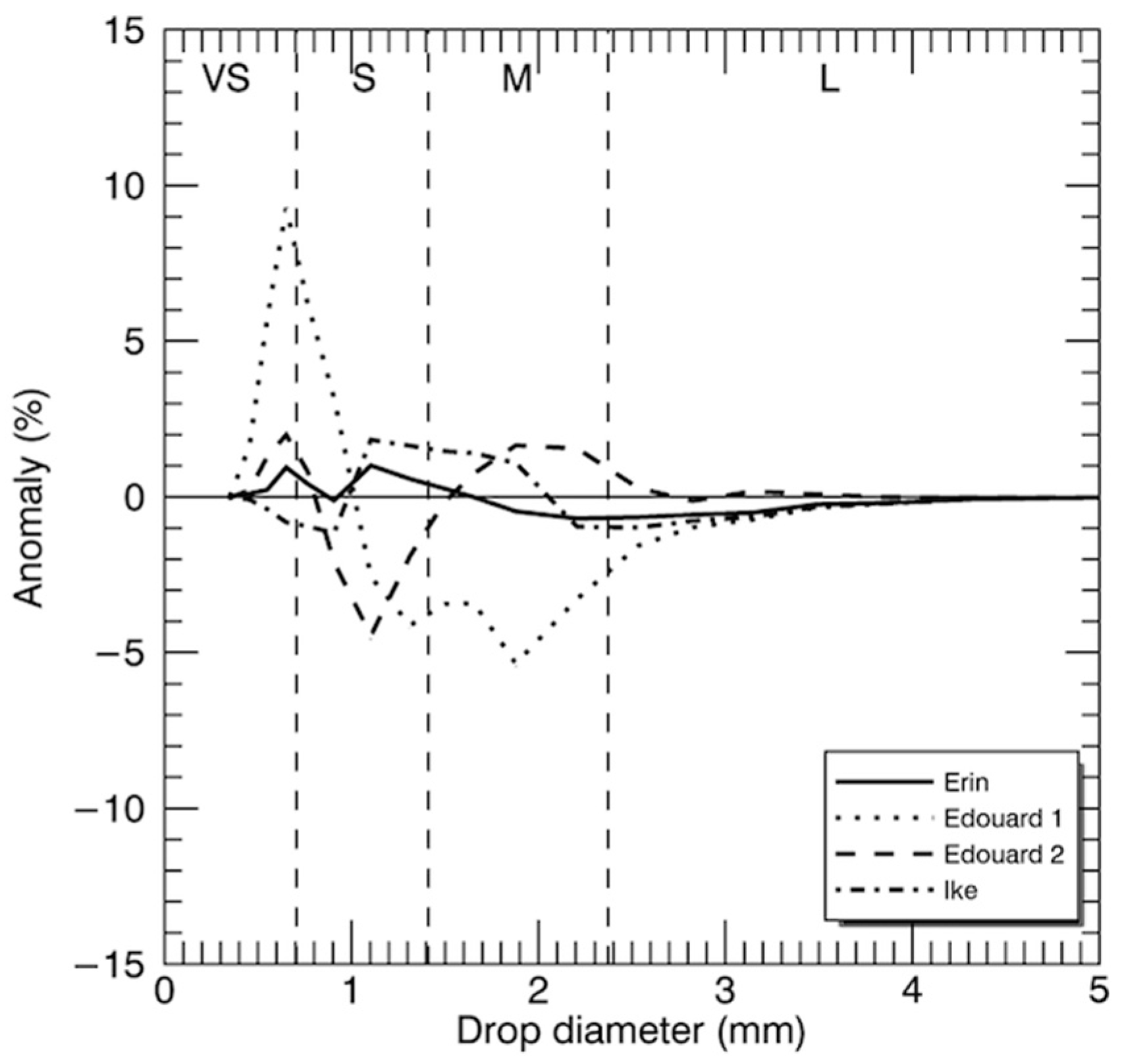
Figure A2.
Representative images for (a) Tropical Storm Erin, (b,c) Tropical Storm Edouard, and (d) Hurricane Ike whose DSDs are presented in Figure A1. The disdrometer location is given by an open circle and the location of the surface low-pressure center is given by the “L” symbol.
Figure A2.
Representative images for (a) Tropical Storm Erin, (b,c) Tropical Storm Edouard, and (d) Hurricane Ike whose DSDs are presented in Figure A1. The disdrometer location is given by an open circle and the location of the surface low-pressure center is given by the “L” symbol.

References
- Hopper, L.J., Jr.; Schumacher, C. Baroclinicity influences on storm divergence and stratiform rain: Subtropical upper-level disturbances. J. Atmos. Sci. 2009, 137, 1338–1357. [Google Scholar] [CrossRef]
- Schultz, D.M.; Schumacher, P.N. The use and misuse of conditional symmetric instability. Mon. Weather Rev. 1999, 127, 2709–2732. [Google Scholar] [CrossRef]
- Houze, R.A., Jr. Stratiform precipitation in regions of convection: A meteorological paradox? Bull. Am. Meteorl. Soc. 1997, 78, 2179–2196. [Google Scholar] [CrossRef]
- Homeyer, C.; Schumacher, C.; Hopper, L.J., Jr. Assessing the applicability of the tropical convective-stratiform paradigm in the extratropics using radar divergence profiles. J. Clim. 2014, 27, 6673–6686. [Google Scholar] [CrossRef] [Green Version]
- Hopper, L.J., Jr.; Schumacher, C. Modeled and observed variations in storm divergence and stratiform rain production in southeastern Texas. J. Atmos. Sci. 2012, 69, 1159–1181. [Google Scholar] [CrossRef]
- Dolan, B.; Fuchs, B.; Rutledge, S.A.; Barnes, E.A. Primary modes of global drop size distributions. J. Atmos. Sci. 2018, 75, 1453–1476. [Google Scholar] [CrossRef]
- Tokay, A.; Short, D.A. Evidence from tropical raindrop spectra of the origin of rain from stratiform versus convective clouds. J. Appl. Meteorl. 1996, 35, 355–371. [Google Scholar] [CrossRef] [Green Version]
- Rao, T.N.; Rao, D.N.; Mohan, K.; Raghavan, S. Classification of tropical precipitating systems and associated Z-R relationships. J. Geophys. Res. 2001, 106, 17699–17711. [Google Scholar] [CrossRef]
- Maki, M.; Keenan, T.D.; Sasaki, Y.; Nakamura, K. Characteristics of the raindrop size distribution in tropical continental squall lines observed in Darwin, Australia. J. Appl. Meteorl. 2001, 40, 1393–1412. [Google Scholar] [CrossRef]
- Zhang, G.; Xue, M.; Cao, Q.; Dawson, D. Diagnosing the intercept parameter for exponential raindrop size distribution based on video disdrometer observations: Model development. J. Appl. Meteorl. Clim. 2008, 47, 2983–2992. [Google Scholar] [CrossRef] [Green Version]
- Waldvogel, A. The N0 jump of raindrop spectra. J. Atmos. Sci. 1974, 31, 1067–1078. [Google Scholar] [CrossRef] [Green Version]
- Houze, R.A., Jr.; Betts, A.K.; Biggerstaff, M.I.; Smull, B.F. Interpretation of Doppler weather-radar displays in midlatitude mesoscale convective systems. Bull. Am. Meteorl. Soc. 1989, 70, 608–619. [Google Scholar] [CrossRef] [Green Version]
- List, R.; McFarquhar, G.M. The role of breakup and coalescence in the three-peak equilibrium distribution of raindrops. J. Atmos. Sci. 1990, 47, 2274–2292. [Google Scholar] [CrossRef] [Green Version]
- McFarquhar, G.M. A new representation of collision-induced breakup of raindrops and its implications for the shapes of raindrop-size distributions. J. Atmos. Sci. 2004, 61, 777–794. [Google Scholar] [CrossRef] [Green Version]
- Rutledge, S.A.; Houze, R.A., Jr. A diagnostic modeling study of the trailing stratiform region of a midlatitude squall line. J. Atmos. Sci. 1987, 44, 2640–2656. [Google Scholar] [CrossRef] [Green Version]
- Steiner, M.; Smith, J.A. Convective versus stratiform rainfall: An ice-microphysical and kinematic conceptual model. Atmos. Res. 1998, 48, 317–326. [Google Scholar] [CrossRef]
- Morrison, H.; Thompson, G.; Tatarskii, V. Impact of cloud microphysics on the development of trailing stratiform precipitation in a simulated squall line: Comparison of one- and two-moment schemes. Mon. Weather Rev. 2009, 137, 991–1007. [Google Scholar] [CrossRef] [Green Version]
- Matejka, T.J.; Houze, R.A., Jr.; Hobbs, P.V. Microphysics and dynamics of clouds associated with mesoscale rainbands in extratropical cyclones. Q. J. R. Meteorl. Soc. 1980, 106, 29–56. [Google Scholar] [CrossRef]
- Disdrometer RD-80. Available online: http://www.ictinternational.com/content/uploads/2018/07/RD-80-Operating-Instructions-January-2015.pdf (accessed on 15 November 2019).
- Joss, J.; Waldvogel, A. Ein spectrograph für niederschlagstropfen mit automatischer auswertung (A spectrograph for raindrops with automatic interpretation). Pure Appl. Geophys. 1967, 68, 240–246. [Google Scholar] [CrossRef]
- Joss, J.; Waldvogel, A. Raindrop-size Distribution and Sampling Size Errors. J. Atmos. Sci. 1969, 26, 566–569. [Google Scholar] [CrossRef] [Green Version]
- Steiner, M.; Smith, J.A. Reflectivity rain rate and kinetic energy flux relations based on raindrop spectra. J. Appl. Meteorl. 2000, 39, 1923–1940. [Google Scholar] [CrossRef]
- Smith, P.L., Jr.; Liu, Z.; Joss, J. A study of sampling-variability effects in raindrop-size observations. J. Appl. Meteorl. 1993, 32, 1259–1269. [Google Scholar] [CrossRef] [Green Version]
- Duchon, C.E.; Essenberg, G.R. Comparative rainfall observations from pit and aboveground rain gauges with and without wind shields. Water Resour. Res. 2001, 37, 3253–3263. [Google Scholar] [CrossRef] [Green Version]
- Tokay, A.; Wolff, D.B.; Wolff, K.R.; Bashor, P. Rain gauge and disdrometer measurements during the Keys Area Microphysics Project (KAMP). J. Atmos. Ocean. Technol. 2003, 20, 1460–1477. [Google Scholar] [CrossRef]
- Habib, E.; Krajewski, W.F.; Kruger, A. Sampling errors of tipping-bucket rain gauge measurements. J. Hydrol. Eng. 2001, 6, 159–166. [Google Scholar] [CrossRef]
- Sheppard, B.E. Effect of irregularities in the diameter classification of raindrops by the Joss-Waldvogel disdrometer. J. Atmos. Ocean. Technol. 1990, 7, 180–183. [Google Scholar] [CrossRef] [Green Version]
- McFarquhar, G.M.; List, R. The effect of curve fits for the disdrometer calibration on raindrop spectra, rainfall rate, and radar reflectivity. J. Appl. Meteorl. 1993, 32, 774–782. [Google Scholar] [CrossRef]
- Steiner, M.; Waldvogel, A. Peaks in raindrop size distributions. J. Atmos. Sci. 1987, 44, 3127–3133. [Google Scholar] [CrossRef] [Green Version]
- Hopper, L.J., Jr. Investigations in Southeast Texas Precipitating Storms: Modeled and Observed Characteristics, Model Sensitivities, and Educational Benefits. Ph.D. Thesis, Texas A&M University, College Station, TX, USA, 2011; 133p. [Google Scholar]
- Johnson, R.H.; Rickenbach, T.M.; Rutledge, S.A.; Ciesielski, P.E.; Schubert, W.H. Trimodal characteristics of tropical convection. J. Clim. 1999, 12, 2397–2418. [Google Scholar] [CrossRef]
- Schaefer, J.T. The life cycle of the dryline. J. Appl. Meteorl. 1974, 13, 444–449. [Google Scholar] [CrossRef]
- Schultz, D.M. Cold fronts with and without prefrontal wind shifts in the central United States. Mon. Weather Rev. 2004, 132, 2040–2053. [Google Scholar] [CrossRef]
- Sanders, F. Real front or baroclinic trough? Weather Forecast. 2005, 20, 647–651. [Google Scholar] [CrossRef]
- Hobbs, P.V.; Matejka, T.J.; Herzegh, P.H.; Locatelli, J.D.; Houze, R.A., Jr. The mesoscale and microscale structure and organization of clouds and precipitation in midlatitude cyclones. I: A case study of a cold front. J. Atmos. Sci. 1980, 37, 568–596. [Google Scholar] [CrossRef] [Green Version]
- Marshall, J.S.; Palmer, W. McK. The distribution of raindrops with size. J. Atmos. Sci. 1948, 5, 165–166. [Google Scholar]
- Fulton, R.A.; Breidenbach, J.P.; Seo, D.-J.; Miller, D.A.; O’Bannon, T. The WSR-88D rainfall algorithm. Weather Forecast. 1998, 13, 377–395. [Google Scholar] [CrossRef]
- Zhang, J.; Howard, K.H.; Langston, C.; Kaney, B.; Qi, Y.; Tang, L.; Grams, H.; Wang, Y.; Cocks, S.; Martinaitis, S.; et al. Multi-Radar Multi Sensor (MRMS) quantitative precipitation estimation: Initial operating capabilities. Bull. Am. Meteorl. Soc. 2016, 97, 621–637. [Google Scholar] [CrossRef]
- MRMS QPE: Hail Caps and Rain Rates. Available online: https://blog.nssl.noaa.gov/mrms/2018/10/hail-caps-and-rain-rates/ (accessed on 27 July 2019).
- Hopper, L.J., Jr.; Schumacher, C.; Stachnik, J.P. Implementation and assessment of undergraduate experiences in SOAP: An atmospheric science research and education program. J. Geosci. Educ. 2013, 61, 415–427. [Google Scholar]
Figure 1.
Comparison of daily rain accumulations between (a) the two tipping bucket rain gauges and (b) the J-W disdrometer and rain gauge average when each instrument is reporting at least 1 mm of rain during August 2005–September 2008 at the College Station, Texas site.
Figure 1.
Comparison of daily rain accumulations between (a) the two tipping bucket rain gauges and (b) the J-W disdrometer and rain gauge average when each instrument is reporting at least 1 mm of rain during August 2005–September 2008 at the College Station, Texas site.

Figure 2.
Climatological drop-size distribution (DSD) normalized by frequency for the four-year study period using all 1-min drop counts ≥ 100. Drop-size modes of very small, small, medium, and large are also identified.
Figure 2.
Climatological drop-size distribution (DSD) normalized by frequency for the four-year study period using all 1-min drop counts ≥ 100. Drop-size modes of very small, small, medium, and large are also identified.

Figure 3.
(a) Individual storm DSD observed on 22 December 2004 and (b) the DSD frequency anomaly for this storm calculated by subtracting the climatological distribution in Figure 2 from (a). Vertical lines show drop-size modes given in Figure 2 (VS: very small, S: small, M: medium, L: large).

Figure 4.
Climatological DSD frequency anomalies for 1-min drop counts ≥ 100 by rain rate.

Figure 5.
DSD anomalies for 1-min drop counts ≥100 by season for December 2004–September 2008 for (a) winter, (b) spring, (c) summer, and (d) fall.
Figure 5.
DSD anomalies for 1-min drop counts ≥100 by season for December 2004–September 2008 for (a) winter, (b) spring, (c) summer, and (d) fall.
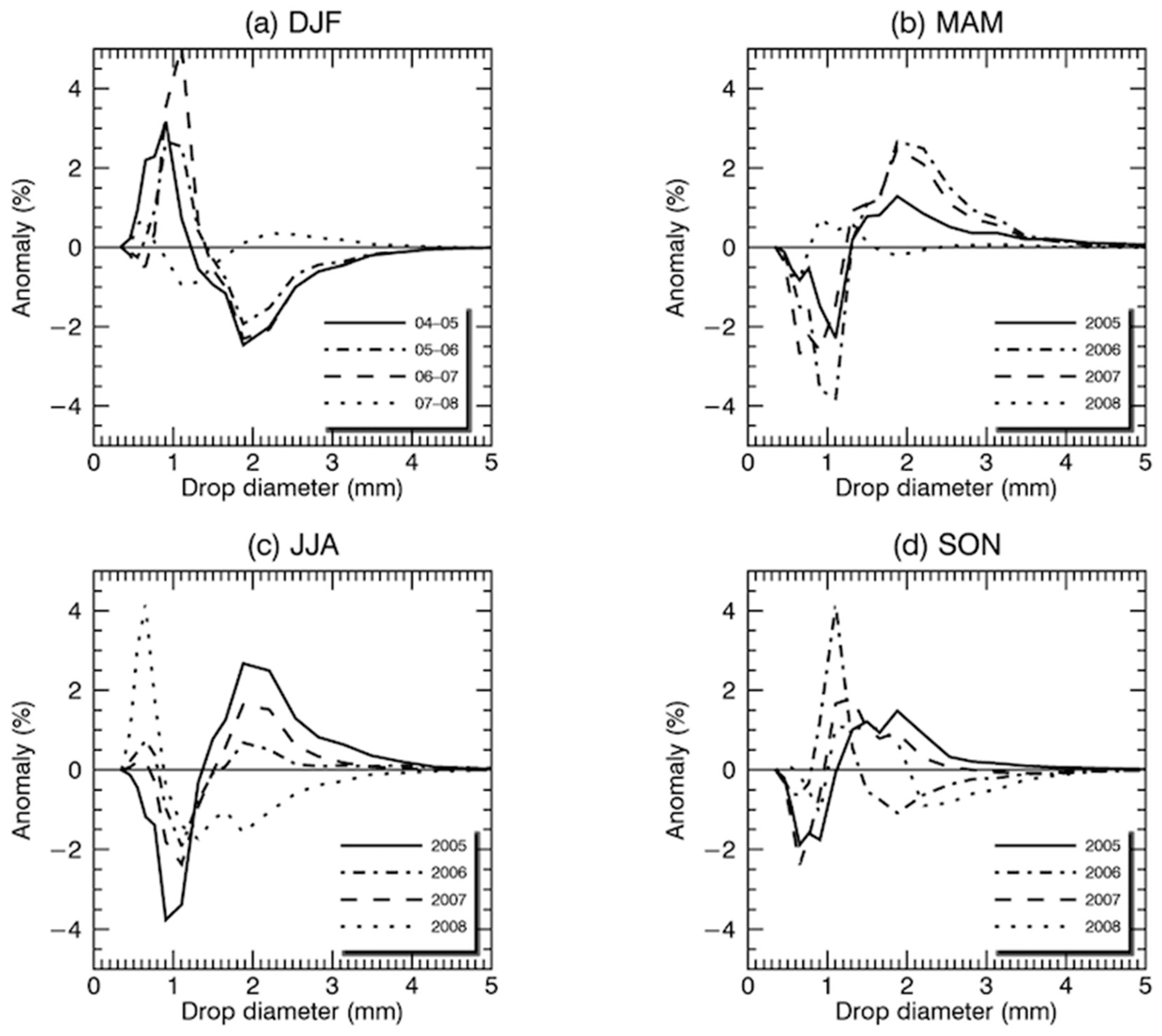
Figure 6.
Examples for predominantly convective (c), deep-convective stratiform (dsf), and non-deep convective stratiform (nsf) structures for: (a–c) cold fronts, (d,e) warm fronts, (f–h) upper-level disturbances, and (i,j) weakly forced storms. The disdrometer location is given by an open circle.
Figure 6.
Examples for predominantly convective (c), deep-convective stratiform (dsf), and non-deep convective stratiform (nsf) structures for: (a–c) cold fronts, (d,e) warm fronts, (f–h) upper-level disturbances, and (i,j) weakly forced storms. The disdrometer location is given by an open circle.
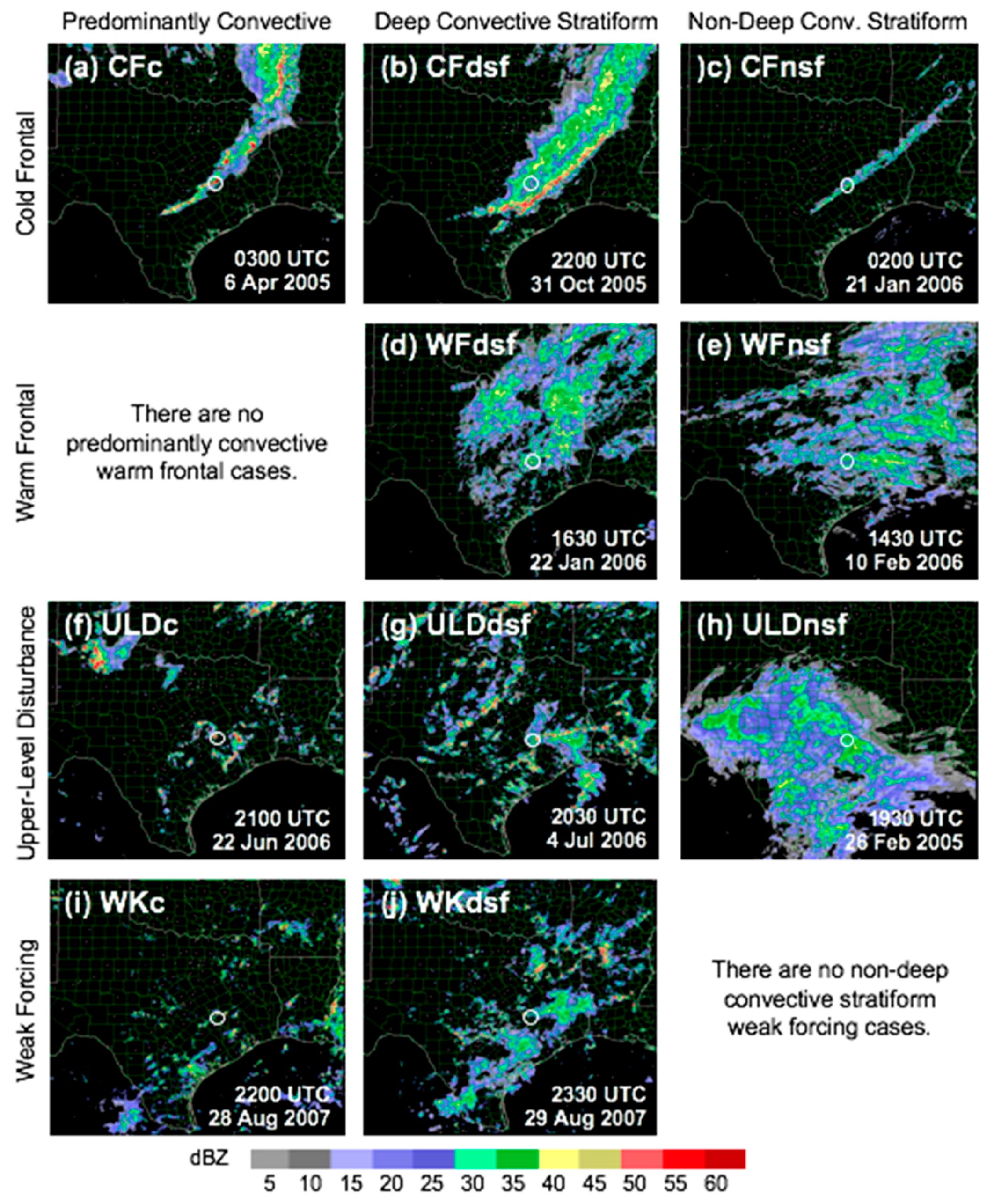
Figure 7.
DSD frequency anomalies for 1-min drop counts ≥ 100 for events associated with weak forcing (WK), cold fronts (CF), warm fronts (WF), and upper-level disturbances (UL).
Figure 7.
DSD frequency anomalies for 1-min drop counts ≥ 100 for events associated with weak forcing (WK), cold fronts (CF), warm fronts (WF), and upper-level disturbances (UL).

Figure 8.
DSD frequency anomalies for 1-min drop counts ≥ 100 for different precipitation structures in (a) weak forcing (WK), (b) cold fronts (CF), (c) warm fronts (WF), and (d) upper-level disturbances (UL). The precipitation factors assigned to the storm types are predominantly deep convective (c), deep-convective stratiform (dsf), and non-deep convective stratiform (nsf).
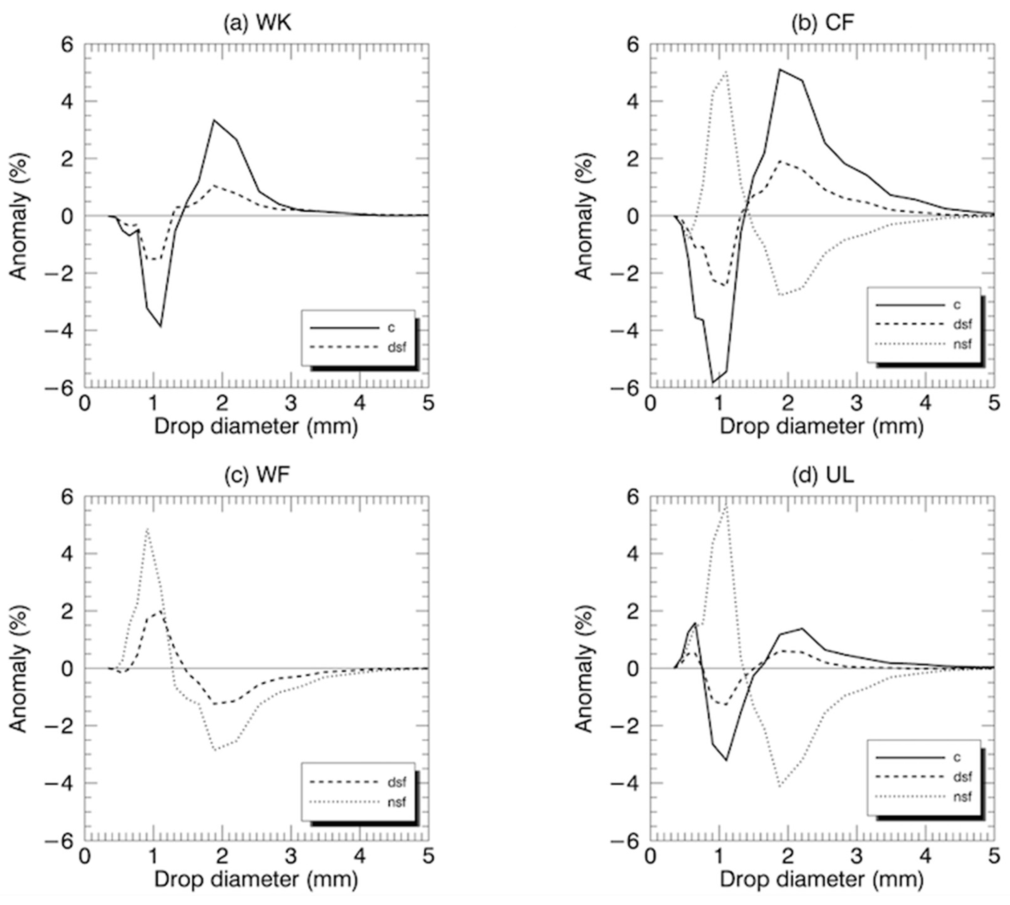
Figure 9.
Z-R relationship parameters a and b for each storm calculated using 1-min DSD spectra with drop counts ≥ 100 for (a) weak forcing, (b) cold frontal, (c) warm frontal, and (d) upper-level disturbance storms. Lines indicate the climatological Z-R relationship (Z = 186R1.63) and red circles indicate the 100-drop storm-type-specific climatological Z-R relationship given in Table 3. For comparison, blue circles indicate the 10-drop storm-type-specific climatological Z-R relationship.


Table 1.
Average diameter of drops in each of the 20 drop-size classes for the Joss–Waldvogel RD-80 (JW) disdrometer.
Table 1.
Average diameter of drops in each of the 20 drop-size classes for the Joss–Waldvogel RD-80 (JW) disdrometer.
| Class | Di (mm) | Class | Di (mm) |
|---|---|---|---|
| 1 | 0.353 | 11 | 1.879 |
| 2 | 0.455 | 12 | 2.207 |
| 3 | 0.549 | 13 | 2.536 |
| 4 | 0.651 | 14 | 2.824 |
| 5 | 0.765 | 15 | 3.145 |
| 6 | 0.906 | 16 | 3.486 |
| 7 | 1.104 | 17 | 3.859 |
| 8 | 1.314 | 18 | 4.286 |
| 9 | 1.496 | 19 | 4.789 |
| 10 | 1.656 | 20 | 5.137 |
Table 2.
Occurrence of storm types for the 163 identified storms, number (#) of 1-min DSD samples per storm type with drop counts ≥ 100, total rainfall, mean storm rainfall, and mean storm duration with their coefficient of variation (CV; standard deviation to mean ratio) observed by the disdrometer.
| Storm Type | # of Storms | # of 1-min Samples | Total Rainfall (mm) | Mean Storm Rainfall (CV) (mm) | Mean Storm Duration (CV) (min) |
|---|---|---|---|---|---|
| Weak Forcing | 12 (7%) | 542 (3%) | 110.4 (4%) | 8.8 (0.91) | 45 (0.89) |
| WKc | 5 | 171 | 37.6 | 7.1 (1.33) | 34 (0.66) |
| WKdsf | 7 | 371 | 72.8 | 10.0 (0.73) | 53 (0.94) |
| Cold Frontal | 76 (47%) | 7488 (41%) | 1282.6 (50%) | 16.1 (0.84) | 99 (0.98) |
| CFc | 17 | 720 | 241 | 13.7 (0.62) | 42 (0.55) |
| CFdsf | 47 | 5106 | 889.7 | 18.0 (0.77) | 109 (0.83) |
| CFnsf | 12 | 1662 | 151.9 | 11.8 (1.43) | 139 (1.06) |
| Warm Frontal | 15 (9%) | 3672 (20%) | 340.5 (13%) | 20.4 (0.68) | 245 (0.63) |
| WFdsf | 10 | 2496 | 249.8 | 22.6 (0.68) | 250 (0.64) |
| WFnsf | 5 | 1176 | 90.7 | 15.9 (0.67) | 235 (0.68) |
| Upper Level | 56 (34%) | 5429 (30%) | 729.2 (29%) | 11.8 (0.89) | 97 (0.84) |
| ULc | 14 | 519 | 113.8 | 7.7 (0.67) | 37 (0.61) |
| ULdsf | 31 | 3218 | 487.2 | 14.4 (0.88) | 104 (0.77) |
| ULnsf | 11 | 1692 | 128.2 | 9.9 (0.76) | 154 (0.57) |
| Tropical Cyclone | 4 (3%) | 1069 (6%) | 95.0 (4%) | 22.2 (0.87) | 267 (0.76) |
| ALL STORMS | 163 | 18,200 | 2557.7 | 14.6 (0.87) | 112 (0.99) |
Table 3.
Storm type average rain rate and Z-R relationships. The rain rate at 40 dBZ based on the storm type Z-R relationship is in the far right column.
Table 3.
Storm type average rain rate and Z-R relationships. The rain rate at 40 dBZ based on the storm type Z-R relationship is in the far right column.
| Storm Type | Average R (mm h−1) | a | b | R at 40 dBZ (mm h−1) |
|---|---|---|---|---|
| Weak Forcing | 5.9 | 170 | 1.58 | 13.2 |
| WKc | 8.5 | 164 | 1.59 | 13.2 |
| WKdsf | 5.1 | 173 | 1.57 | 13.2 |
| Cold Frontal | 4.5 | 188 | 1.63 | 11.4 |
| CFc | 10.2 | 184 | 1.63 | 11.6 |
| CFdsf | 4.8 | 210 | 1.61 | 11.0 |
| CFnsf | 2.0 | 163 | 1.55 | 14.2 |
| Warm Frontal | 2.4 | 179 | 1.68 | 11.0 |
| WFdsf | 2.7 | 183 | 1.68 | 10.8 |
| WFnsf | 1.8 | 174 | 1.66 | 11.5 |
| Upper Level | 3.0 | 190 | 1.61 | 11.7 |
| ULc | 5.0 | 159 | 1.63 | 12.7 |
| ULdsf | 3.8 | 201 | 1.60 | 11.5 |
| ULnsf | 1.4 | 185 | 1.59 | 12.3 |
| Tropical Cyclone | 3.0 | 183 | 1.62 | 11.8 |
| ALL STORMS | 3.5 | 186.4 | 1.63 | 11.5 |
| NEXRAD | 300 | 1.40 | 12.2 |
Table 4.
Comparison of rainfall amounts by storm type. The measured rainfall is accumulated from one-minute disdrometer-derived rain rates. The percent error from the measured rainfall is presented for the climatological Z-R (Z = 186R1.63), the Z-R relationship calculated for each storm type (see Table 3), and the NEXRAD Z-R relationship (Z = 300R1.4). Bold values indicate the best estimate.
| Storm Type | J-W Rainfall (mm h−1) | Climatological Z = 186R1.63 % Error | Storm Type Z-R % Error | NEXRAD Z = 300R1.4 % Error |
|---|---|---|---|---|
| Weak Forcing | 110.4 | 13.6 | −0.3 | 0.7 |
| WKc | 37.6 | 12.6 | −1.8 | −1.2 |
| WKdsf | 72.8 | 14.1 | −0.2 | 1.7 |
| Cold Frontal | 1283 | 2.9 | 3.5 | −8.3 |
| CFc | 241 | 3.8 | 3.2 | −17.9 |
| CFdsf | 889.7 | 0.7 | 4.7 | −10.4 |
| CFnsf | 151.9 | 14.4 | −1.5 | 19.7 |
| Warm Frontal | 341 | −5.6 | −2.4 | −3.3 |
| WFdsf | 249.8 | −6.6 | −1.7 | −7.1 |
| WFnsf | 90.7 | −2.9 | −4.7 | 7.0 |
| Upper Level | 729 | 1.5 | −0.2 | −2.9 |
| ULc | 113.8 | 6.0 | −3.6 | −9.4 |
| ULdsf | 487.2 | 1.1 | 1.3 | −5.1 |
| ULnsf | 128.2 | −0.8 | −4.4 | 11.5 |
| Tropical Cyclone | 95 | 3.6 | 1.3 | 8.9 |
| ALL STORMS | 2558 | 1.9% | 1.4% | −5.0% |
© 2019 by the authors. Licensee MDPI, Basel, Switzerland. This article is an open access article distributed under the terms and conditions of the Creative Commons Attribution (CC BY) license (http://creativecommons.org/licenses/by/4.0/).
Share and Cite
MDPI and ACS Style
Hopper, L.J., Jr.; Schumacher, C.; Humes, K.; Funk, A. Drop-Size Distribution Variations Associated with Different Storm Types in Southeast Texas. Atmosphere 2020, 11, 8. https://doi.org/10.3390/atmos11010008
AMA Style
Hopper LJ Jr., Schumacher C, Humes K, Funk A. Drop-Size Distribution Variations Associated with Different Storm Types in Southeast Texas. Atmosphere. 2020; 11(1):8. https://doi.org/10.3390/atmos11010008
Chicago/Turabian StyleHopper, Larry J., Jr., Courtney Schumacher, Karen Humes, and Aaron Funk. 2020. "Drop-Size Distribution Variations Associated with Different Storm Types in Southeast Texas" Atmosphere 11, no. 1: 8. https://doi.org/10.3390/atmos11010008
Note that from the first issue of 2016, this journal uses article numbers instead of page numbers. See further details here.