Article

Assimilation of Radar Data, Pseudo Water Vapor, and Potential Temperature in a 3DVAR Framework for Improving Precipitation Forecast of Severe Weather Events

1
School of Atmospheric Sciences, Nanjing University of Information Science and Technology, Nanjing 210044, China
2
Hubei Key Laboratory for Heavy Rain Monitoring and Warning Research, Institute of Heavy Rain, China Meteorological Administration, Wuhan 430205, China
3
NOAA National Severe Storms Laboratory, Norman, OK 73072, USA
*
Authors to whom correspondence should be addressed.
Atmosphere 2020, 11(2), 182; https://doi.org/10.3390/atmos11020182
Submission received: 1 January 2020 / Revised: 4 February 2020 / Accepted: 6 February 2020 / Published: 9 February 2020
(This article belongs to the Special Issue Radar Hydrology and QPE Uncertainties)

Abstract

:
An improved approach to derive pseudo water vapor mass mixing ratio and in- cloud potential temperature was developed in this paper to better initialize numerical weather prediction (NWP) and build convective-scale predictions of severe weather events. The process included several steps. The first was to identify areas of deep moist convection, utilizing Vertically Integrated Liquid water (VIL) derived from a mosaicked 3D radar reflectivity field. Then, pseudo- water vapor and pseudo- in- cloud potential temperature observations were derived based on the VIL. For potential temperature, the latent heat initialization for stratiform cloud and moist adiabatic initialization for deep moist convection were used based on a cloud analysis method. The third step was to assimilate the derived pseudo- water vapor and potential temperature observations, together with radar radial velocity and reflectivity into a convective-scale NWP model during data assimilation cycles spanning several hours. Finally, 3-h forecasts were launched each hour during the data assimilation period. The effects of radar data and pseudo- observation assimilation on the prediction of rainfall associated with convective systems surrounding the Meiyu front in 2018 were explored using two real cases. Two sets of experiments, each including several experiments in each real case, were designed to compare the effects of assimilation radar and pseudo- observations on the ensuing forecasts. Relative to the control experiment without data assimilation and radar experiment, the analyses and forecasts of convections were found to be improved for the two Meiyu front cases after pseudo- water vapor and potential temperature information was assimilated.

1. Introduction

Because the current conventional observations network cannot provide sufficient information to accurately initialize the convective-scale numerical weather prediction (NWP) model, a lot of research has focused on using radar data to improve the convective-scale NWP over the past decades [1,2,3,4,5,6,7,8,9,10,11,12,13,14]. However, in the NWP model, only wind and hydrometeor variables can be directly related to radar observations, and other model variables cannot be directly observed by radars.
It is relatively easy to assimilate radar radial velocity into the NWP model, but it is difficult to assimilate reflectivity because the relationship between the radar reflectivity and model hydrometeor variables is nonlinear. Yet, the effective assimilation of reflectivity into convective-scale models is essential for properly initializing convective-scale NWP models. One simple way to assimilate reflectivity data for initializing the convective-scale NWP is the cloud analysis method [15,16,17,18,19]. For example, the Advanced Regional Prediction System (ARPS [20]) cloud analysis [18] can specify hydrometeor variables and adjust in-cloud temperatures for the initialization. Although this method has been proven useful, problems still remain. One problem is that the cloud analysis method relies on empirical algorithms to relate the hydrometeor variables and the reflectivity, and requires tuning of many uncertain parameters [7]. Another problem is that too much water vapor and latent heating are added to the cloud analysis, resulting in an increased false alarm rate and over-prediction, especially when many data assimilation cycles are involved [21,22,23]. To solve these problems, more data assimilation approaches have been used, such as latent heat nudging [24], variational techniques [1,7,8,9,10,11,25,26], the ensemble Kalman filter (EnKF) [5,6,12,27,28,29], and hybrid variational and ensemble approaches [13,14,30]. These studies have demonstrated that assimilation of reflectivity can improve short-term forecasts. However, the quality of predictions is still not reasonable in many cases because of the lack of key observations in convective scale NWP, especially water vapor mixing ratios and potential temperature perturbations, which are essential for accurate forecasts [31].
Realizing the important role of water vapor in convective scale NWP, many studies have focused on assimilating pseudo- water vapor (qv), or relative humidity (RH) observations derived in different ways [9,25,26,32,33,34,35,36,37,38,39]. For example, Caumont et al. [25] and Wattrelot et al. [26] developed a 1D + 3DVAR method in Meteo-France mesoscale model. Using a Bayesian inversion method, the RH profile was retrieved from the observed reflectivity and assimilated as pseudo- observations in the 3DVAR system. The application of this technique in convection-allowing models showed notable improvements in the short-term forecasts of accumulated precipitation [25]. Wang et al. [10] designed a scheme to estimate in-cloud qv and cloud water from radar reflectivity, and assimilated these pseudo- observations into the Weather Research and Forecasting Model (WRF) model. Results also showed that assimilating in- cloud RH pseudo- observations had an obviously positive impact on the short-term precipitation simulation of summer convective events. Fierro et al. [34,35,36] developed nudging and the 3DVAR assimilation method to assimilate the pseudo- qv which was derived from total lightning density fields observed by either the ground-based Earth Networks Total Lightning Network (ENTLN) or the space-borne Geostationary Lightning Mapper (GLM [40]). These assimilation methods of lightning data showed that the effect of assimilation of lightning data and radar reflectivity on the improvement of prediction is generally the same. The results indicated that assimilating lighting data through a pseudo- qv observation operator in a 3DVAR system notably improved the short-term forecast of severe weather events in terms of the timing and location of the observed convections [34,36].
In Lai et al. [39], hereafter L19, the Vertically Integrated Liquid water (VIL) [41] calculated from the observed reflectivity and background reflectivity was used to identify deep moist convection regions for each field, and pseudo- qv observations were derived in these regions based on a convective stratiform segregation method proposed by Zhang and Qi [42]. The pseudo-qv observations were then assimilated into a convective-scale NWP model along with radar data using a 3DVAR system [7,8]. It was demonstrated that moisture was enhanced in the convection regions and was reduced in the spurious cell regions. The short-term (≤0–3 h) forecasts were improved based on results of two real data cases. However, thermal-dynamical variables which are also very important for convective scale NWP [31], were not initiated in L19.
The purpose of the present study is to investigate how to properly initialize the thermal-dynamical variables in the convective scale NWP model. Built on L19, a convective–stratiform segregation method was used to separate areas for the deep convective cloud and stratiform cloud. Pseudo in-cloud potential temperature observations were then derived using the diabatic initialization [15,16,17] in the areas for the stratiform cloud, and moist adiabatic initialization [18] in the areas for the convective cloud, respectively. The method is applied to two Meiyu front convective events on 30 June 2018 and 4 July 2018, over the middle range of Yangtze River in China, and the results are compared with the pseudo-qv approach implemented in L19.
The rest of this study is organized as follows: In Section 2, we give a brief description of the 3DVAR system and the detail method of pseudo- qv and potential temperature based on the VIL. In the Section 3, the design of experiments is described. Results of two cases are presented in Section 4. Finally, summary and conclusion are followed in Section 5.

2. Methodology and Data

2.1. General Description of a 3DVAR System

In this study, a 3DVAR data assimilation system developed especially for convective scale data assimilation was used [2,3,7,8,18]. The cost function defined in the 3DVAR system included three terms: background, observation, and weak constraint. The analysis variable contained three wind components (u, v and w), potential temperature (θ), pressure (p), water vapor mixing ratio (qv) and hydrometeor mixing ratios (rainwater qr, snow qs and hail qh). The observations included the radar radial velocity, reflectivity and derived pseudo observations. The mass continuity equation was used as a weak constraint. Detailed description of 3DVAR cost function, velocity, and reflectivity observation operator can be found in [3,7,8]. The forward observation operator for radial velocity considers the effects of the Earth’s curvature and includes the three-dimensional wind components. The forward operator for reflectivity is obtained by summing the contributions from rain, snow and hail mass mixing ratios based on classified hydrometeor types using background temperature. The recursive filter proposed by Purser et al. [43,44] is used to model the effect of the background error covariance. Considering the variations of observation density, multiple analysis passes are used to assimilate different observation types with different filter scales [45,46]. In this study, three passes (with length scales of 24 km, 12 km, and 4 km, respectively) were used in the recursive filter.

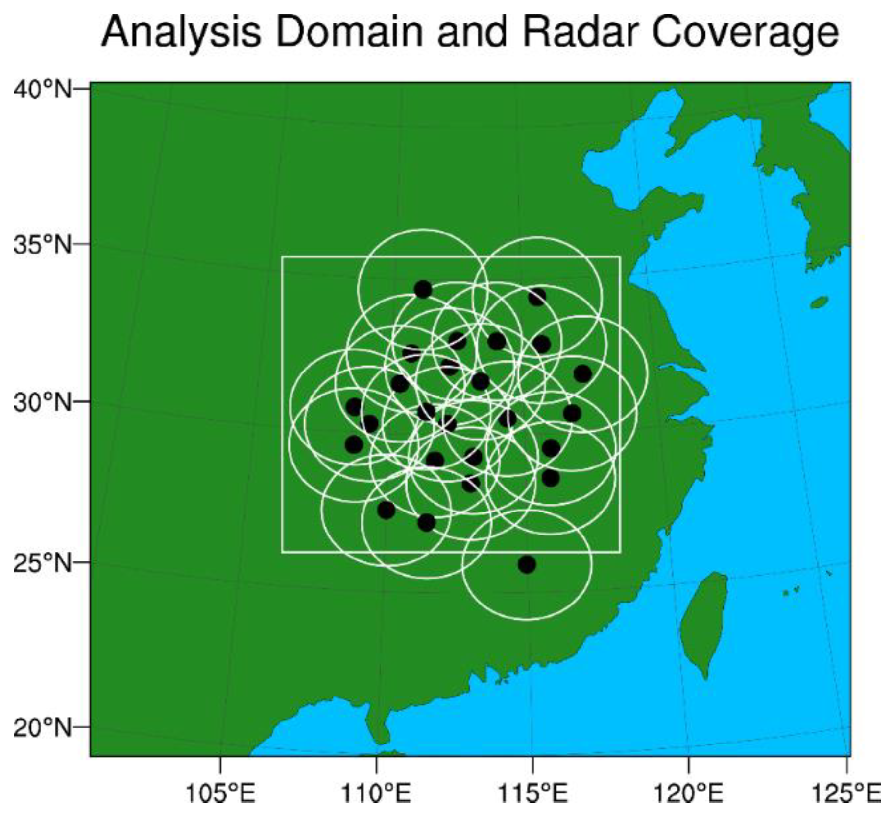
2.2. Radar Data and Quality Control

In this study, radar level-II data from China New Generation Weather Radar (CINRAD) network were used. The CINRAD network consists of more than 200 radars, including S-Band and C-band instruments manufactured by three companies [47]. The selected scan strategy was VCP21 in which nine elevations 0.5°, 1.5°, 2.4°, 3.4°, 4.3°, 6.0°, 9.9°, 14.6°, 19.5°were used for scanning every 6 min. The range gate resolution was 250 m for radial velocity and 1000 m for reflectivity, and azimuthal gate resolution was about 1.0 degree for both. Quality control is very important for appropriate use of these radar data in convective scale data assimilation and short-term forecasts. Radar data quality control including calibration, non-meteorological echo filtering and velocity dealiasing was done by using the Severe Weather Automatically Nowcast System (SWAN) [47,48,49,50]. After the quality control step, the radar reflectivity data were projected to the model grids to form the three-dimensional gridded reflectivity data. If reflectivity data from multiple radars overlap at a given grid point, the largest value is picked. Other details about the processing and quality control of Doppler radar data are described in Gao et al. [8].

2.3. The Pseudo- Water Vapor Mixing Ratio Observations Derived by VIL

In this section, we briefly introduce the pseudo- qv observations derived by VIL in the reference L19. The most important aspect of this method is to use the VILs derived from observed radar reflectivity to identify areas of deep moist convection [42]. The detail routine of creating the pseudo- qv can be found in L19 [Figure 1]. First, the VILs were calculated from the three-dimensional gridded observed reflectivity data merged from multiple radars by a radar pre-processing routine and from the reflectivity field from the model output, respectively. Then, the convective-stratiform segregation method [42] was employed to separate areas of the convections from areas of stratiform columns. If an empirical VIL threshold (a default value of 6.5 kg m−2) in both the observed and model simulated reflectivities is met, the column is classified as “convective”; if not, it is classified as “stratiform”. Second, the relative humidity in the identified convective columns was set at saturation (namely RH = 100%) between the lifted condensation level (LCL) and a fixed “cloud top” height determined by a fixed reflectivity threshold of 18.5 dBZ according to Klazura and Imy [51]. Third, sometimes the background contains spurious convections where the observed reflectivity indicates stratiform columns or “no- rain” echoes. In order to account for this problem, two scenarios were considered. One is to compress the spurious convections in the background field. That is to reduce the RH to 95% of the background above of the LCL when the VILs derived from background field are bigger than 6.5 kg m−2, but the VILs from observations are less than 6.5kg km−2. Another scenario is to reduce the relative humidity in the areas of spurious convections in the background field where the observations show “no-rain”. At the same time, in order to avoid an over-moisturizing initial field, the RH is reduced by half of the difference between the background relative humidity and a reference RH value in areas where reflectivity is larger than 20 dBZ in the background. Except for the above two scenarios, the RH of the background was not modified due to the uncertainty of the relationship between RH and reflectivity. Finally, the pseudo- qv observations were calculated in the layer between the lifted condensation level and special top level. As pointed out in L19, there were three sources of uncertainties for the pseudo- qv observations derived from the RH profiles. They are related to the accuracy of identifying the ‘deep moisture’ region, the pressure and temperature fields in the background field, and issues in RH adjustment. In order to reduce these uncertainties, the observation error for the pseudo- qv was set at 3.0 g/kg, a relatively large value used by Fierro et al. [35].

2.4. The Pseudo- in-Cloud Potential Temperature Observations

Temperature perturbations associated with precipitation clouds play a very important role in sustaining existing convection because latent heating is a dominant component in the total diabatic heating [52]. However, they cannot be directly observed. Latent heating profiles differ substantially between areas of stratiform, deep convective, and shallow precipitation [52,53,54]. In general, two in-cloud thermal adjustments are used in convective scale models. One is the diabatic latent-heating scheme, in which the temperature adjustment is calculated from the latent heat release associated with the added hydrometeors [15,16,17]. The other is the moist-adiabatic temperature adjustment scheme, in which a moist-adiabatic temperature profile with the same entrainment factor as applied to the cloud water is used to adjust the temperature after determination of cloud and precipitation contents [18]. This moist-adiabatic scheme was used to initialize convective storms for the ARPS model [20]. For convective storms, the moist-adiabatic scheme is more appropriate because it reflects the temperature change in an ascending moist air parcel [18]. However, in reality, the convective cloud and stratiform cloud may coexist in a single Mesoscale Convective System (MCS). Here, following L19, we proposed to derive pseudo- in-cloud temperature observations based on VILs introduced in the above sub-section. If VILs are greater than a threshold (a default value of 6.5 kg m−2) in an observed storm, the model column is classified as “convective” and pseudo- in-cloud temperature observations are derived using the moisture adiabatic initialization scheme [18]. Otherwise, if VILs are smaller than the threshold, the model column is classified as stratiform precipitation and uses the diabatic latent heating scheme that is suitable for stratiform precipitation [15]. Similar to the pseudo- qv, the pseudo- potential temperature (θ) also contains some uncertainty. Thus, we set the observation error to 4 K, which is larger than that for observations from radiosonde.

3. Case Descriptions and Experimental Design

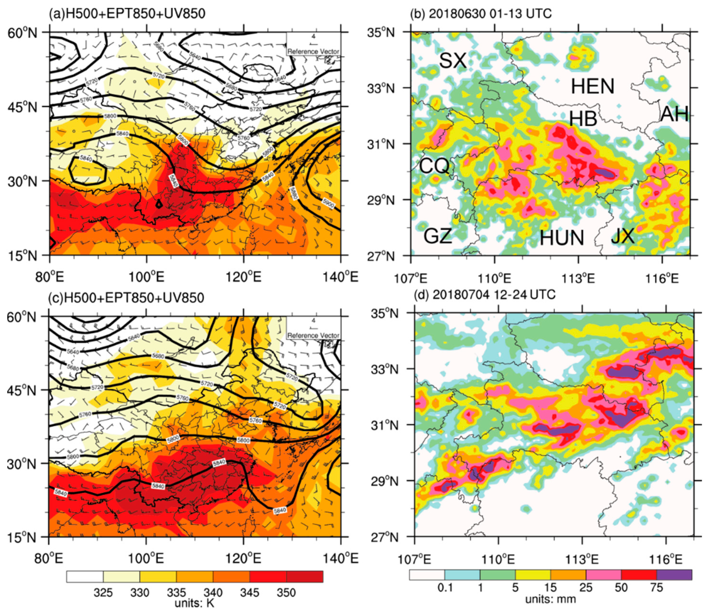
3.1. Case Description

The Meiyu front (called Meiyu in China, Baiu in Japan, and Changma in Korea) is one of the most important components in the East Asian Summer Monsoon system as it always associates with mesoscale convective complexes (MCCs) or mesoscale convective systems (MCSs) that propagate eastward along the baroclinic zone [55,56]. Accurate quantitative precipitation forecast (QPF) of Meiyu heavy rainfall events from a numerical weather prediction model remains a difficult problem. Although there are a lot of successful simulations of the Meiyu front, the location, time, pattern, and amount of precipitation is hard to predict successfully. Yet, the accurate forecast when and where the MCSs are triggered and of their subsequent evolution are critical to improve the QPF associated with the Meiyu front. Thus, in this study, we choose to investigate the impact of assimilating radar data and pseudo- observations on the prediction of QPF with two Meiyu front cases. These two cases are typical Meiyu front events and occurred in East Asia in 2018.

3.1.1. Case 1: 30 June 2018

On 30 June 2018, heavy rainfall with more than 50 mm/day rate lashed the southern part of Hubei Province in middle Yangtze River. This rainfall event was associated with a Meiyu front, which is typical over the middle and lower reaches of the Yangtze River in early summer. At 0000 UTC 30 June 2018, a northeast-southwest oriented upper-air trough was located in East China, with the trough bottom in the middle of the Yangtze River Valley (Figure 1a). Such upper-air dynamical conditions were not favorable for the development of an upper level divergence over Hubei Province. However, at 850 hPa, a quasi-west-east oriented wind shear line appeared over the mid-lower Yangtze River Valley, promoting low-level convergence and a mid-level ascending motion (Figure 1a). To the south of the shear line, warm and moisture air was transported by a southwest flow from the Bay of Bengal. The large gradient of equivalent potential temperature over the mid-lower Yangtze River Valley indicated the convergence of warm and moist air from the south with dry air from the north. Therefore, a rainstorm developed with collective influence from the low-level shear line and surface Meiyu front. As southward migration of the low-level shear line and Meiyu front began, this heavy rainfall event over Hubei was brought to end after 0700 UTC on 30 June.

3.1.2. Case 2: 4 July 2018

Another Meiyu front-associated heavy rainfall event occurred on 4 July 2018. The spatial distribution of 12-h accumulated precipitation (shown in Figure 1d) exhibited a southwest-northeast oriented rain belt. Heavy rainfall (exceeding 25 mm/12 h) mainly existed in the junction of Hubei, Hunan and Chongqing, central and northeastern part of Hubei, southeastern part of Henan and northern part of Anhui. Hourly precipitation evolution (not shown) was characterized by a long narrow northeast-southwest-oriented rain belt migrating eastward slowly, in which several MCSs with precipitation rate exceeding 10 mm/h were observed.
This heavy precipitation event was collectively influenced by upper-level trough/ridge and low-level shear line. At 1200 UTC on 4 July 2018 (Figure 1c), there was an India-Burma trough at 500 hPa. Meanwhile, a ridge was observed over Hetao Plain. The southwest flow ahead of the India-Burma trough and the northwest flow ahead of the Hetao ridge converged over the mid-lower Yangtze River Valley, which was favorable for frontal genesis over this region. Similar to the event that occurred on 30 June 2018, a remarkable low-level shear line existed over the mid-lower Yangtze River Valley, suggesting favorable moisture and dynamical conditions for heavy precipitation in this region. By comparing Figure 1c,d, it was found that the rain belt was located almost exactly along the 850 hPa shear line. The high equivalent potential temperature (exceeding 350 K) at 850 hPa within the rain belt suggested the accumulation of unstable energy, which would lead to convection development and strong hourly rainfall along the rain belt (Figure 1d).

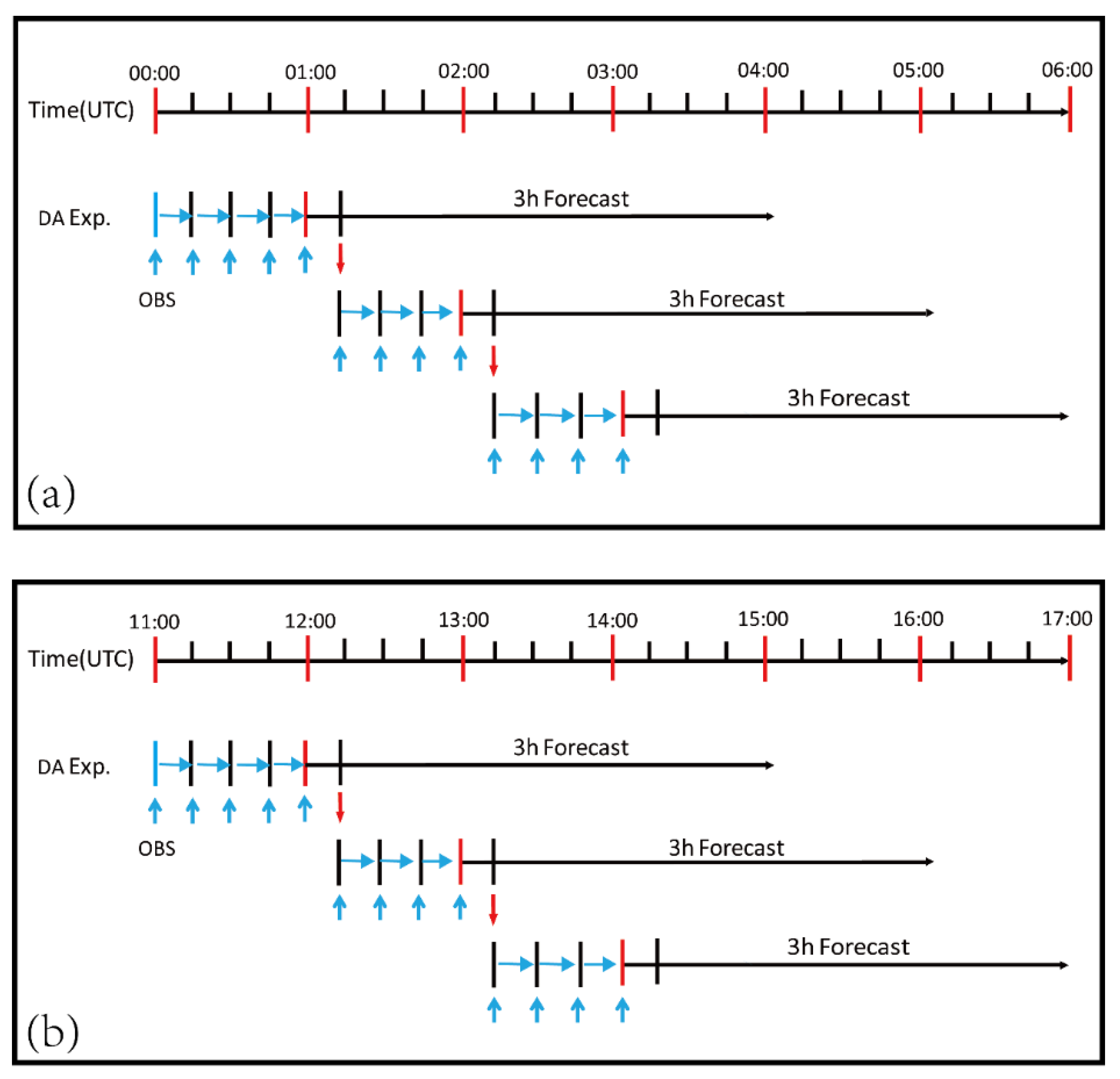
3.2. Model and Experimental Design

The numerical model used for this study is the three-dimensional compressible nonhydrostatic Weather Research and Forecasting model (version 3.7.1) with Advanced Research WRF dynamic core (WRF-ARW) [57]. This model has been used in a broad range of applications across scales ranging from meters to thousands of kilometers and in both weather and climate research communities. The model physics parameterization schemes employed in this study include the Thompson microphysics scheme [58], the Yonsei University (YSU) planetary boundary layer scheme (PBL) [59], the Dudhia shortwave radiation scheme [60], and the rapid radiative transfer model (RRTM) longwave radiation scheme [61]. The cumulus parameterization scheme was not used. In this study, the model domain size for both cases was 800 × 700, with a grid horizontal resolution of 1.5 km. The center of the model domain was at (31.0° N, 112.3° E) (Figure 2). The stretched vertical grid has 51 levels with a top set at 50 hPa. The time step for the model integration was 6 s.
As stated in the last section, the observations in this study included radial velocity, reflectivity, pseudo- qv, and pseudo- θ observations. There were 25 radars from the operational CINRAD network inside the analysis domain for both Case 1 and Case 2 (Figure 2). To investigate the impact of assimilating both radar and the pseudo- observations on the Meiyu front rainfall forecasts, five experiments were conducted for each case (Table 1). For the 30 June 2018 case, the control run did not assimilate any observations, named C1CTL. Experiment C1Rad assimilated radar radial velocity, reflectivity, and surface data. Experiment C1RadPQ was done by adding the assimilation of pseudo- qv data in addition to the data used in C1Rad. Experiments C1RadPQPT1 and C1RadPQPT2 assimilate radar, surface, pseudo- qv, and pseudo- θ data. The difference between the C1RadPQPT1 and C1RadPQPT2 is that the former assimilates pseudo- θ derived from only moisture adiabatic scheme, and the later from the proposed scheme described in Section 2.4. The same set of five experiments was performed for the second case as well (Table 1).
The diagram of data assimilation cycles and forecast cycles for two cases is shown in Figure 3. For Case 1 (2), the model was cold-started at 0000 UTC (1100 UTC), and data assimilation was cycled with 15 min interval for 3 h until 0300 UTC (1400 UTC). Three-hour forecasts were launched from 0100 UTC (1200 UTC), 0200 UTC (1300 UTC), and 0300 UTC (1400 UTC) for Case 1 (2).The National Centers for Environmental Prediction (NCEP) Global Forecast System (GFS) forecast product at 0.25 degree resolution from 1800 UTC 29 June 2018 (0600 UTC 4 July 2018) to 1800 UTC 30 June 2018 (0300 UTC, 5 July 2018) at a 3-h interval were interpolated into our model domain (Figure 2) for the purpose of providing initial background field and boundary conditions for the data assimilation cycles and short-term forecasts.

4. Results and Discussion

In this section, the performance of assimilating radar data and pseudo- observations (pseudo- qv and pseudo- θ) on the QPF for the two Meiyu front cases is evaluated by comparing the model precipitation and composite reflectivity field against observations.

4.1. 30 June 2018 Case

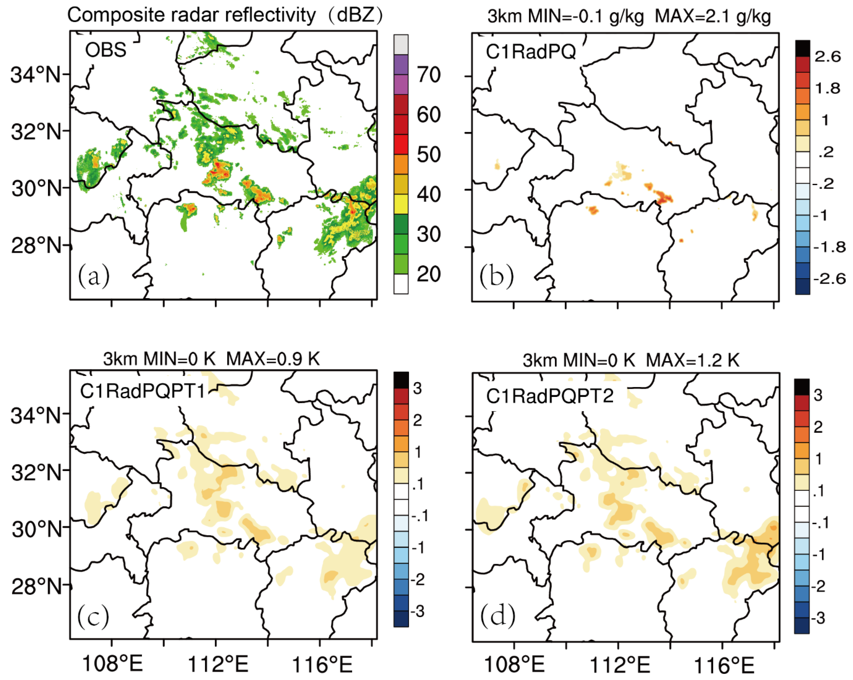
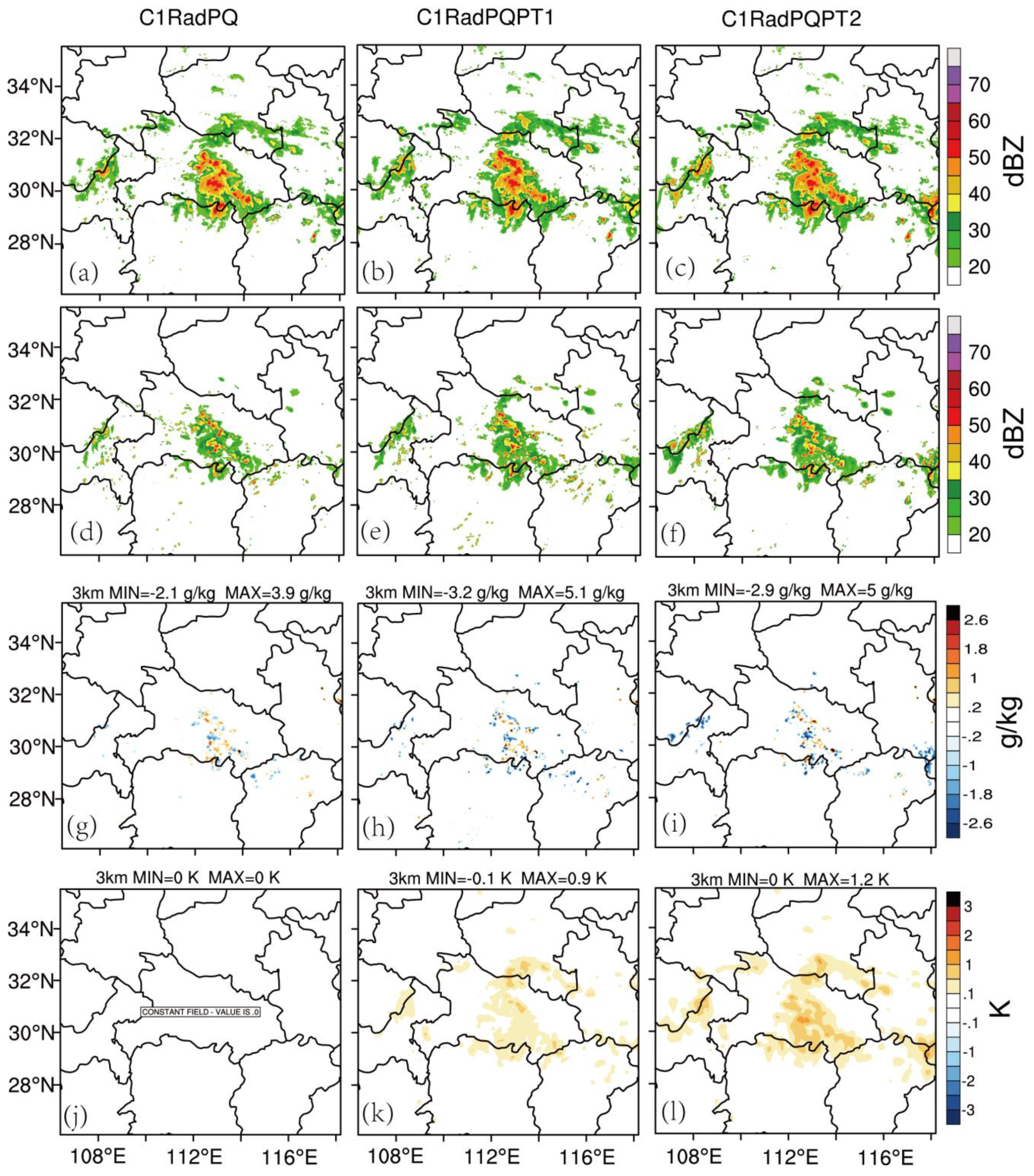
4.1.1. Impact on the Analysis Fields

First, we discuss the impact of assimilating the pseudo- qv and pseudo- θ observations on the analysis fields for this case. The water vapor increment areas for experiment C1RadPQ at the center of the model domain exist where large observed radar echoes appear (Figure 4a vs. Figure 4b) with a maximum value for qv increment about 2.1 g kg−1 and minimum value of about −0.1 g kg−1. Qv increments for both C1RadPQPT1 and C1RadPQPT2 have very similar patterns as the C1RadPQ at this time (not shown). As for θ, the increments have larger and wider areas than water vapor field, which is consistent with the observed reflectivity coverage in both C1RadPQPT1 and C1RadPQPT2 (Figure 4c,d). It is worth noting that the pattern of θ increments for two pseudo- θ experiments are similar but the details are not the same, e.g., C1RadPQPT2 has warmer areas in the observed strong reflectivity regions, especially at an area near the east boundary, which is mainly dominated by the stratiform precipitation. It is reasonable because the C1RadPQPT2 takes advantages of both latent heating and the moist adiabatic scheme.
After 3 h into the data assimilation cycles, the separated convective systems merge and form a MCS in all three experiments: C1RadPQ, C1RadPQPT1, and C1RadPQPT2 (Figure 5a–c). The analyzed reflectivity fields are roughly consistent with the observed reflectivity fields for all three experiments, and are stronger than the background composite reflectivity fields (Figure 5d–f). The positive qv increment areas are mainly located in the strong radar reflectivity regions, while the negative qv increment areas are collocated with spurious reflectivity in the analysis (Figure 5g–i). The maximum (minimum) values of the qv increments for C1RadPQ, C1RadPQPT1, and C1RadPQPT2 are about 3.9 (−2.1) g kg−1, 5.1 (−3.2) g kg−1, and 5.0 (−2.9) g kg−1, respectively. Thus, the adjustments for qv in C1RadPQPT1, and C1RadPQPT2 are larger than that in C1RadPQ. At this time, the relatively big positive increments for θ at 0300 UTC are mainly located in the MCS area. For the newly created convection at the southeast of Henan, the increment patterns for the two pseudo −θ experiments are almost same (Figure 5k,l). It is worth noting that the θ increments in C1RadPQPT2 are larger than that in the C1RadPQPT1 where reflevtivities are greater than 40 dBZ. This is due to the θ increments from two sources, one is from the deep moisture convections, and another is from the stratiform precipitation in the MCS. The moist-adiabatic scheme for convections heats the atmosphere through a greater depth with larger amplitude, while the latent heating scheme warms the atmosphere more at the middle and lower levels with less amplitude (not shown). This could potentially lead to more accurate forecasts, as will be demonstrated later.

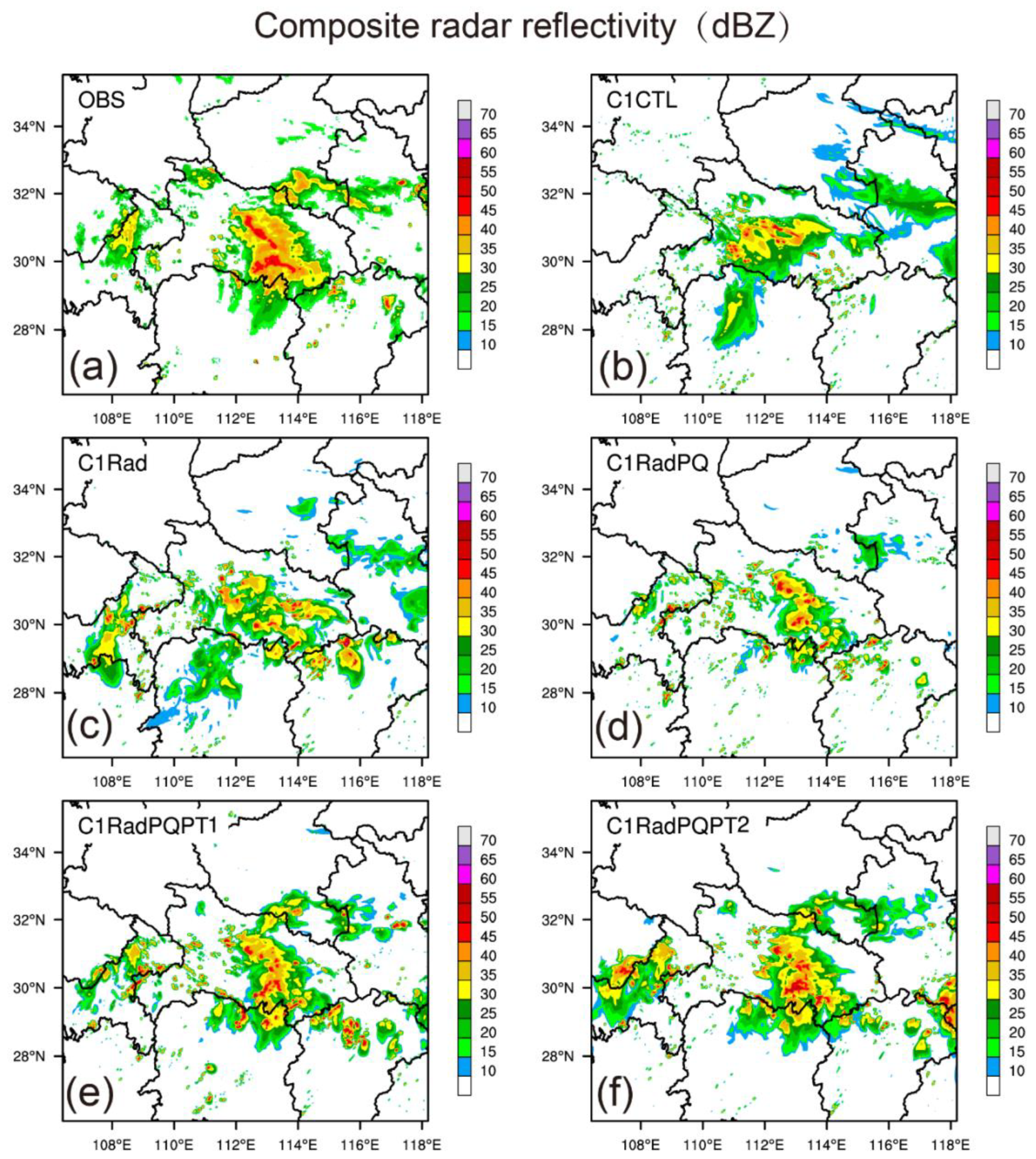
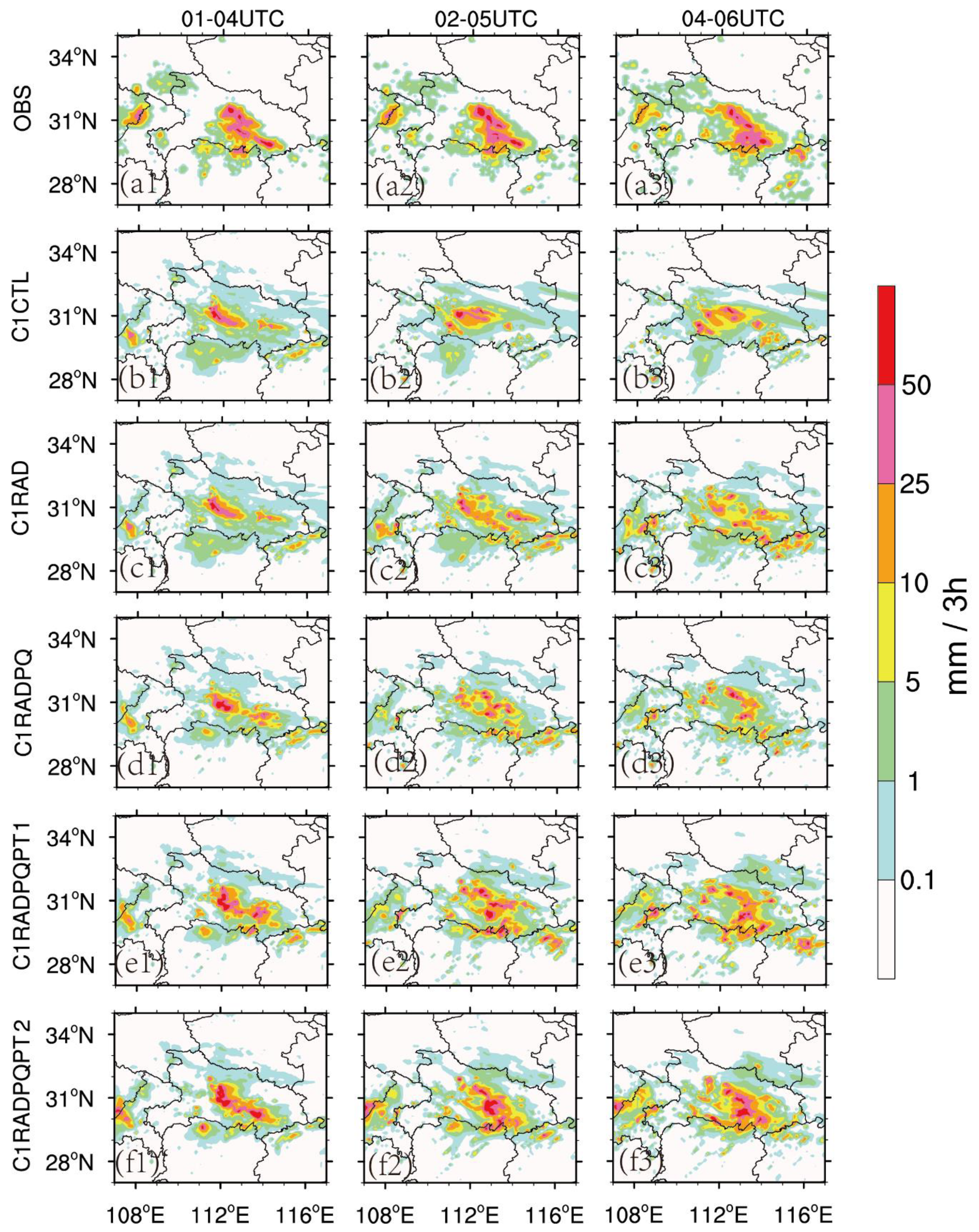
4.1.2. Qualitative Forecast Evaluation

To evaluate the impact of assimilating pseudo- observations on the forecast fields of the MCS, the radar reflectivity fields simulated by the five experiments are compared with 3D radar reflectivity mosaic product by SWAN [48]. One hour into the forecast launched from 0300 UTC, the area and reflectivity amplitude of MCS became stronger than that at the 0300 UTC (Figure 6a vs. Figure 5a). The strong composite reflectivity region in C1CTL is 50–100 km further west than observed (Figure 5a vs. Figure 5b). After assimilating the radar data (including radar velocity and reflectivity), the pattern of the reflectivity is a little closer to the observations, especially at the southeast of the Hubei province (Figure 6c). The location and intensity of the convections are improved and the scatter convection bulbs become more organized for C1RadPQ (Figure 6d). This is because the assimilation of pseudo- qv enhances the convections in the middle of the Hubei province and also suppresses the spurious convections in the southwest domain. The assimilation of the pseudo- θ in addition to pseudo- qv helps predict the convections in the south of the Henan province. More organized MCS is predicted in the centre of the domain (Figure 6e,f). Especially in C1RadPQPT2, the MCS is better organized than those in other experiments (Figure 6f). Three hours into the forecast, only the reflectivity pattern and amplitude in C1RadPQPT2 were closer to the observations and maintain an MCS structure (Figure 7). This indicates that the newly proposed scheme used in C1RadPQPT2 is more efficient and useful for precipitation forecast than the others.
To provide a complete picture of forecast performance, the 0–3 h accumulated precipitation forecast at each cycle is also evaluated (Figure 8). To get rid of the influence of lateral boundary on precipitation simulation, we only quantitatively and qualitatively evaluate the accumulated precipitation within subdomains (27–35° N, 107–117° E). The precipitation observations are produced by a method called CMORPH (NOAA CPC Morphing technique) [62]. It merges hourly precipitation observed by automatic weather stations (AWS) in China and satellite data 0.1°∗0.1° temporal-spatial resolution through the two-step merging algorithm of PDF (probability density function) and OI (optimal interpolation) [62]. All predictions in the comparisons are at a 10-km resolution, with verification data remapped from 1.5-km grids.
The observed product shows that precipitation occurred mainly in the middle of Hubei province (Figure 8a1–3). The 3-h precipitation in C1CTL is further west and weaker than that observed (Figure 8b1–3). The 3-h accumulated precipitation in C1Rad at 0300 UTC is better than that in the first two cycles. However, the location and amount of 3-h accumulated precipitation for C1RadPQPT1 and C1RadPQPT2 are significantly better than the other two experiments in comparison with observations in the first cycle (Figure 8a1,e1,f1). In the last two cycles, the C1RadPQPT2 had better performance than all the other experiments (Figure 8f2,3. This indicates that simultaneously assimilating radar data and pseudo- observations can notably improve the 3-h accumulated precipitation forecasts.

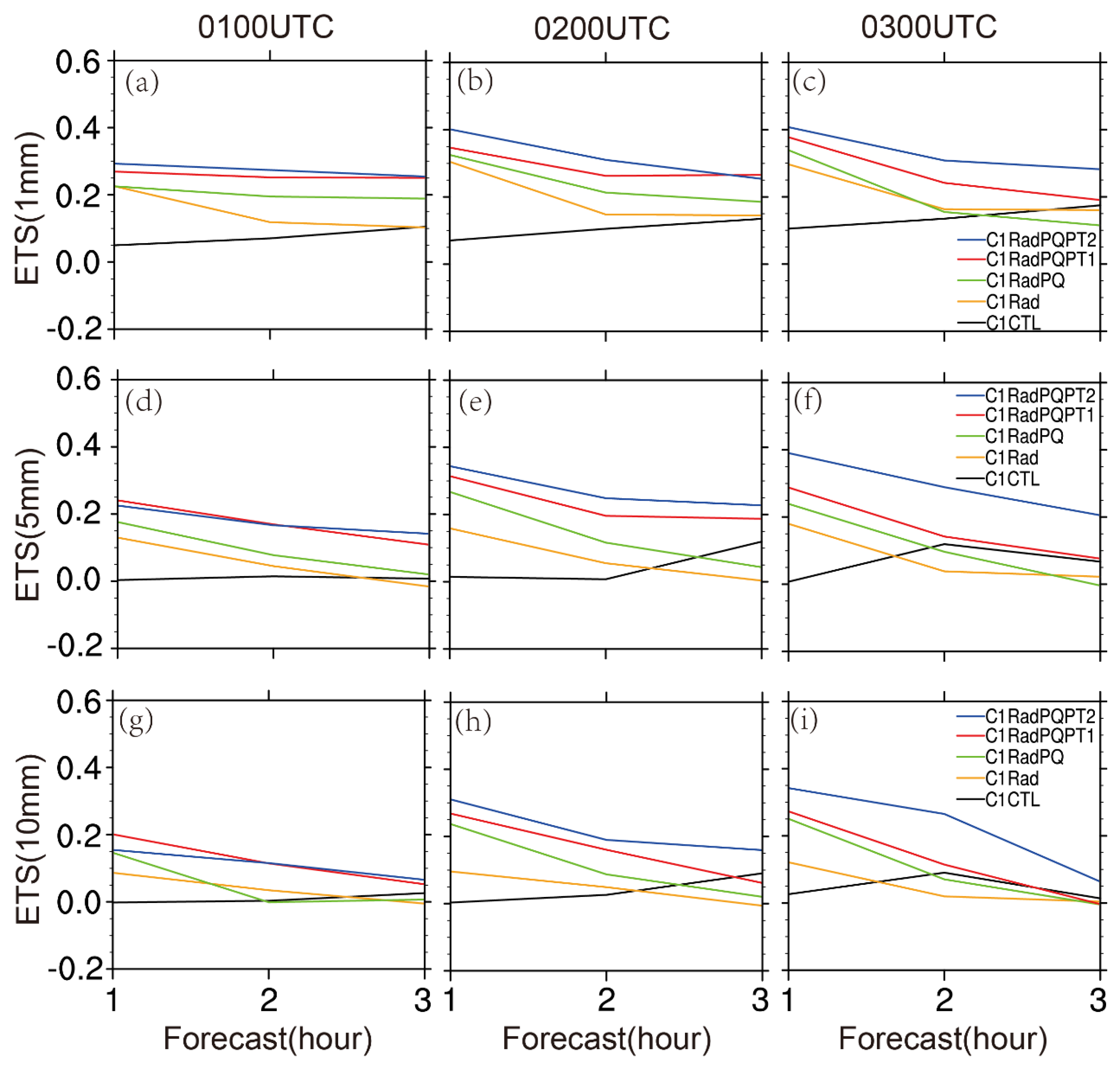
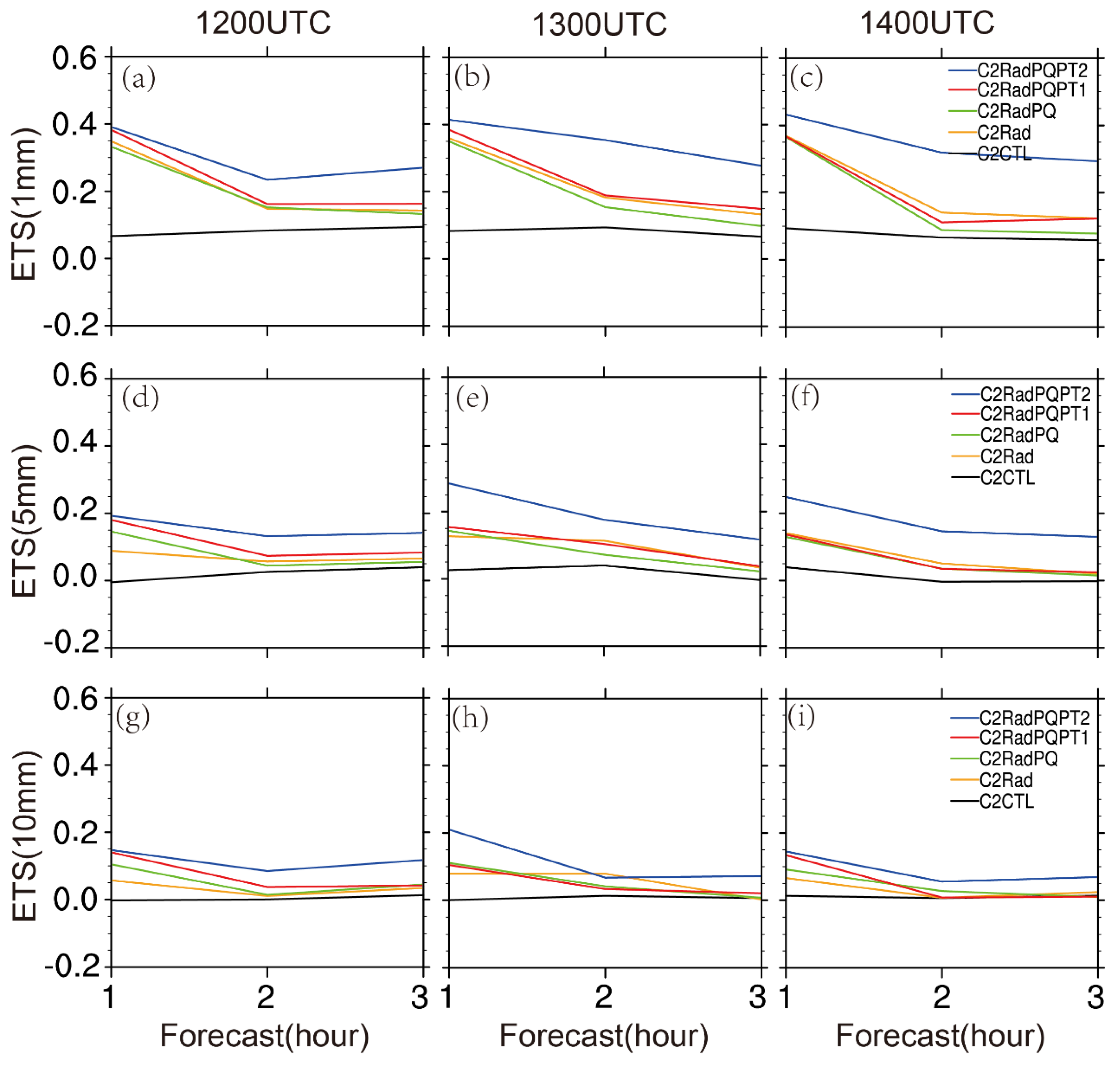
4.1.3. Quantitative Evaluation

Based on the encouraging qualitative results, the equitable threat scores (ETS) [63] of 1-h accumulated precipitation are calculated for quantitative evaluation of the performance of assimilation experiments. The ETS is widely used for evaluating NWP forecast results. The ETS is calculated on a gridpoint basis, satisfying or exceeding a defined threshold (e.g., 1-h accumulated precipitation), the value of 1.0 indicating a perfect forecast and less than 0.0 indicating no forecast skill.
The ETS is calculated for 1-h accumulated precipitation at 1, 5, and 10 mm for the 30 June 2018 case (Figure 9). It shows that the ETS values for assimilation of both pseudo- qv and pseudo- θ in C1RadPQPT2 are superior for almost all 0–3 h forecasts, except that the forecast for the first cycle for 5 mm and 10 mm precipitation thresholds. In general, all experiments with either pseudo-qv only or both pseudo- qv and pseudo- potential temperature improve QPF.

4.2. 4 July 2018 Case

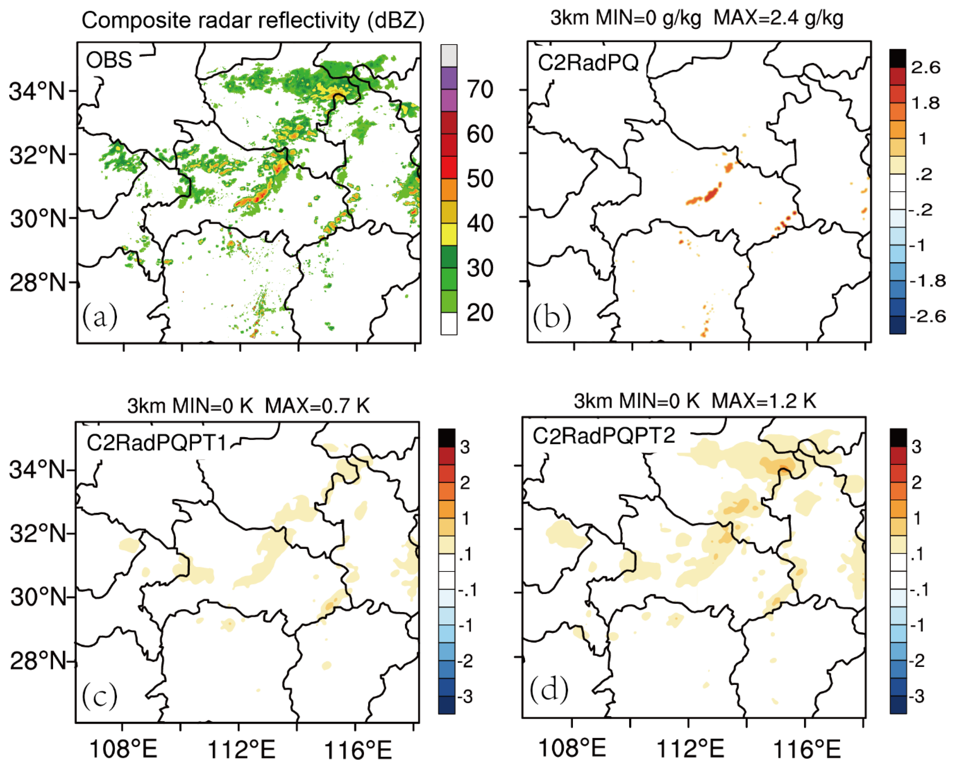
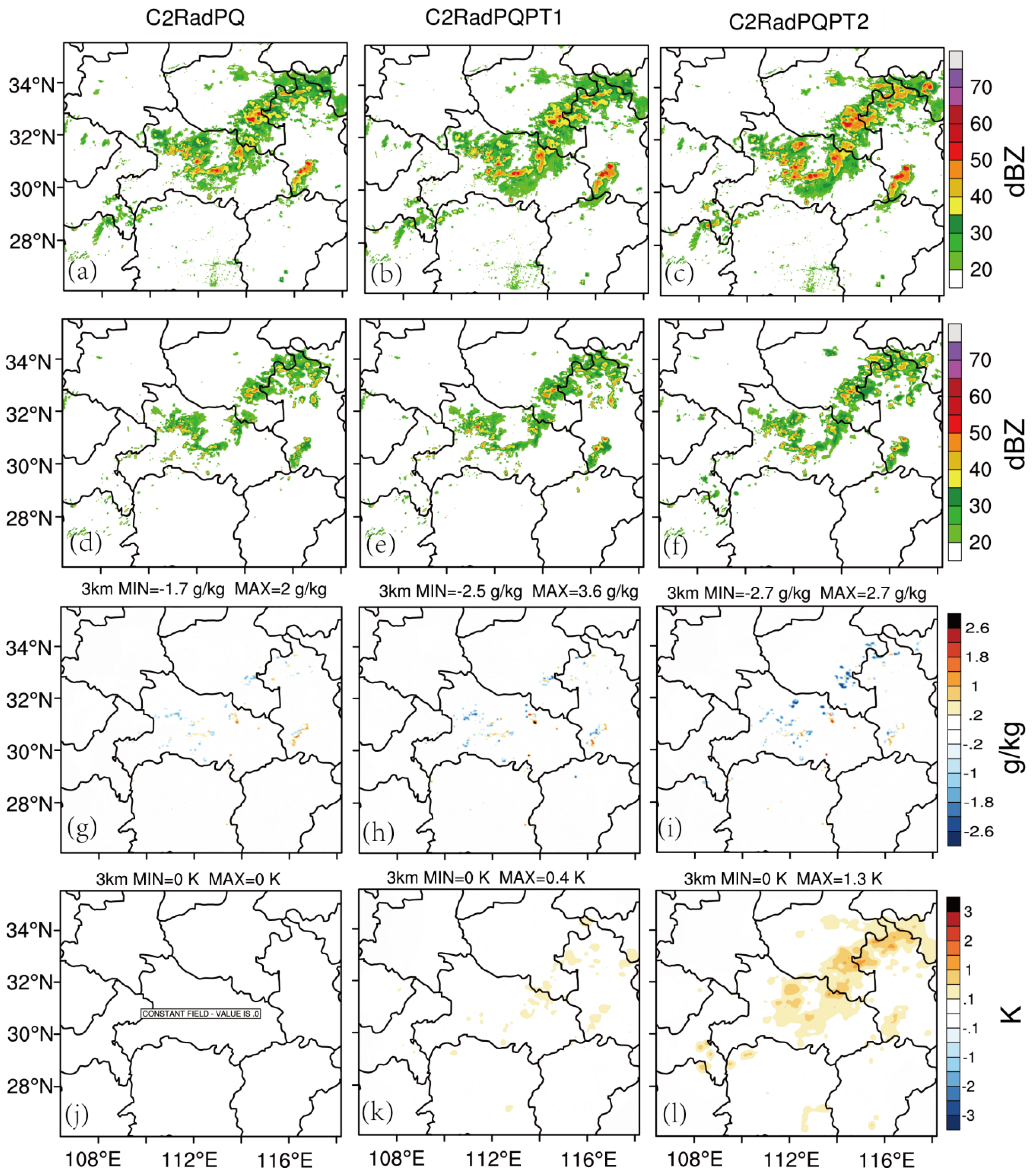
4.2.1. Impact on the Analysis Fields

Similar to Case 1, the analyzed qv increments for C2RadPQ, θ increments for C2RadPQPT1 and C2RadPQPT2, and the observed composited reflectivity at 3 km above-ground-level (AGL) for 1100 UTC are shown in Figure 10. The large water vapor (qv) increments for C2RadPQ is mainly located at the center of the model domain, where large observed radar echoes exist (>35 dBZ) with maximum value about 2.4 g kg−1 (Figure 10b). The areas for θ increments in the C2RadPQPT1 roughly collocate with the areas for composite reflectivities with values larger than 35 dBZ, while the areas for θ increments in C2RadPQPT2 are wider and bigger than that in C2RadPQPT1. This is quite similar to the first case.
At 1400 UTC (3 h into the data assimilation cycles), the convections are weaker (stronger) in Hubei (Henan) province. The analyzed reflectivity patterns (Figure 11a–c) generally improve for background reflectivity patterns (Figure 11d–f). The qv increments for C2RadPQ, C2RadPQPT1 and C2RadPQPT2 have similar patterns, although the C2RadPQPT2 have more negative coverage areas (Figure 11g–i). The θ increments in C2RadPQPT2 (Figure 11l) are stronger and wider than that in C2RadPQPT1 (Figure 11k), similar to the first case.

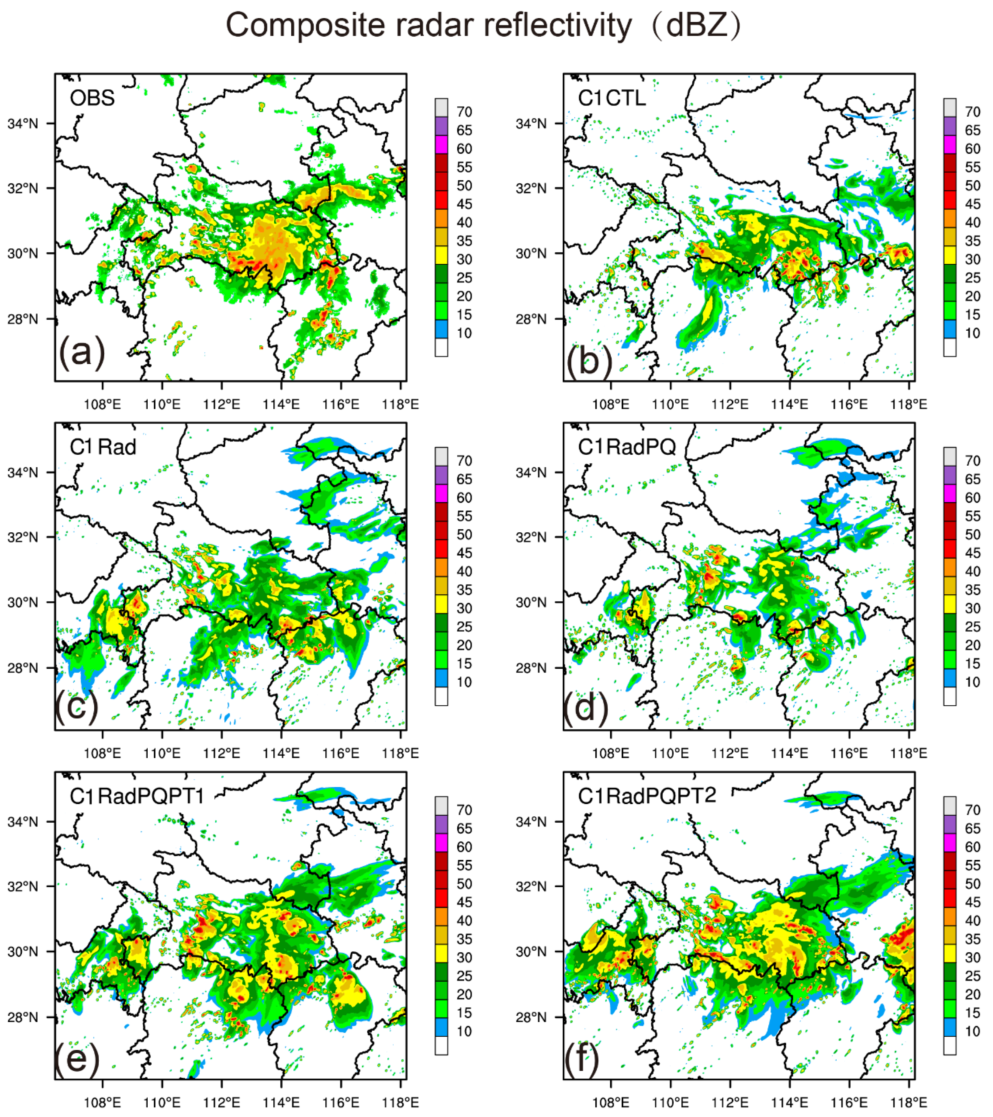
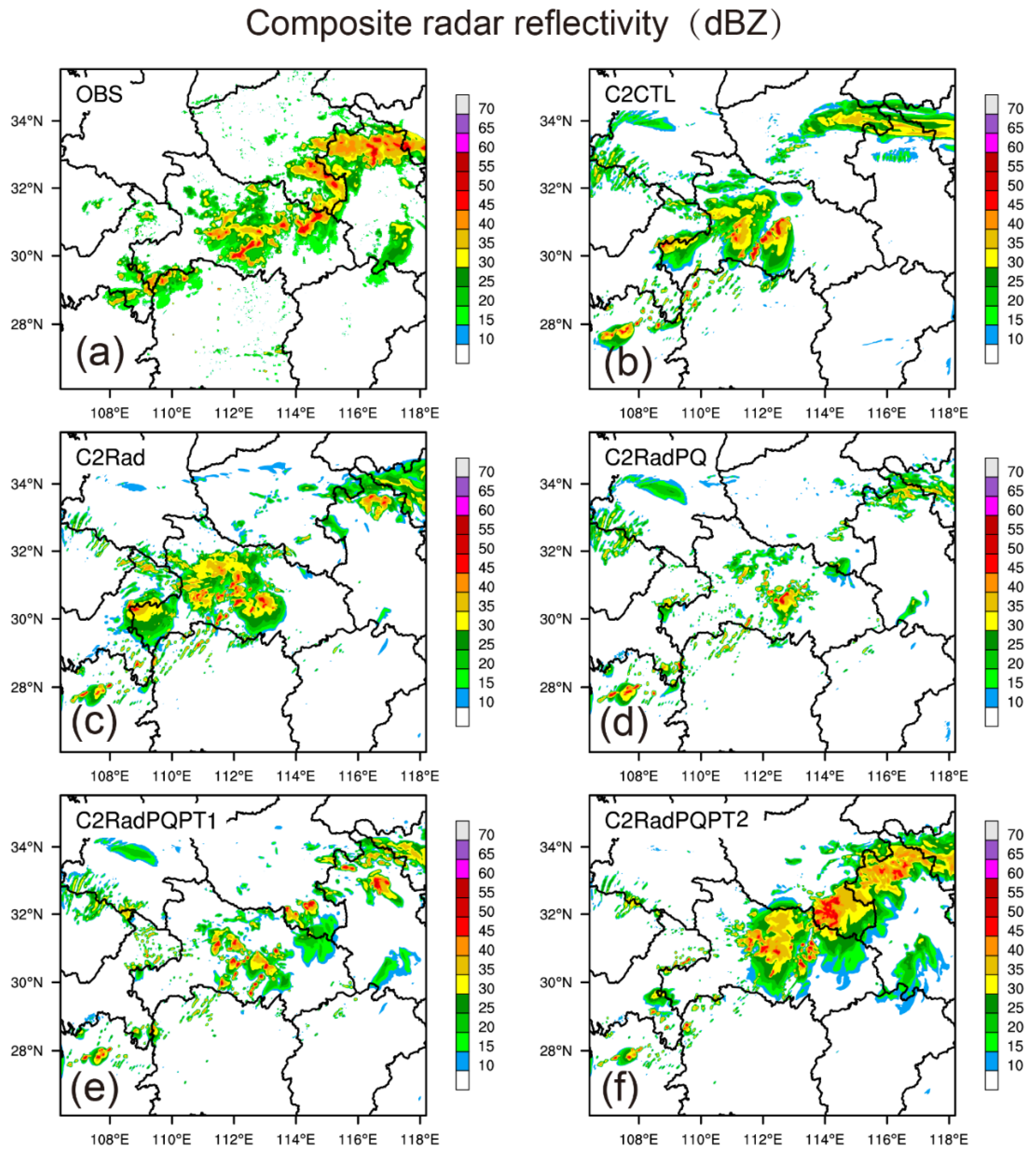
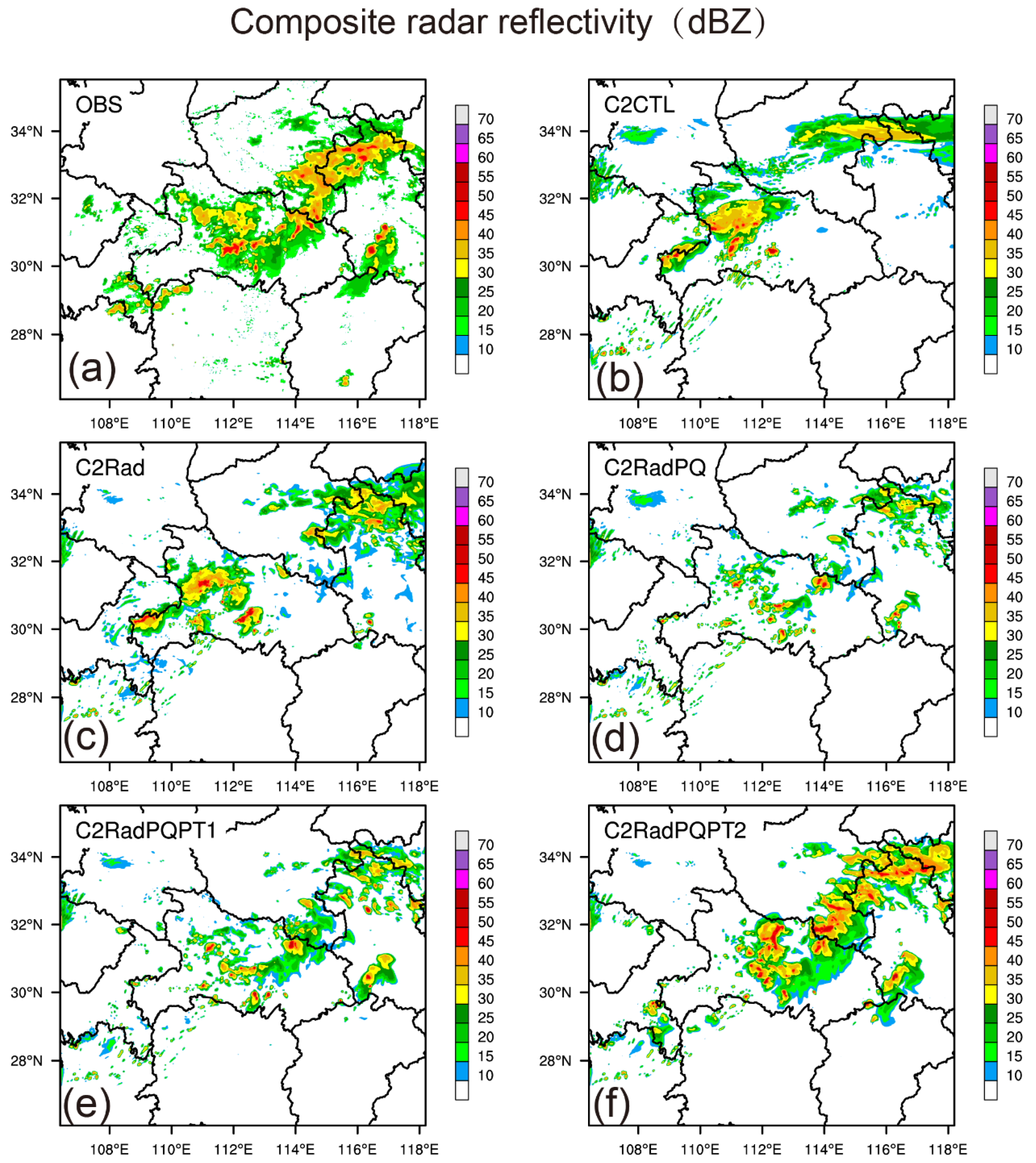
4.2.2. Qualitative Forecast Evaluation

Similar to Case 1, 1-h and 3-h simulated composite reflectivity for all five experiments are evaluated (Figure 12 and Figure 13). At 1500 UTC, the southwest-northeast oriented patterns of composite reflectivity associated with the Meiyu front were observed (Figure 12a). One hour into the forecast, only partial reflectivity field is predicted in C2CTL (Figure 12b). The C2Rad has some improvement in the northeast part in Henan and Anhui provinces (Figure 12c). Only experiment C2RadPQPT2 can successfully predict the orientation of the MCS and effectively suppress spurious cells (Figure 12f).
At 1700 UTC, the Meiyu front rain belt was oriented northeast-southwest from Hubei to Anhui province (Figure 13a). Although C2CTL was able to capture the storm in the middle of Hubei, it was not in the right location (Figure 13b). The simulated composite reflectivity was weakest in C2RadPQ (Figure 13d), and strongest in C2RadPQPT2 (Figure 13f). None of the five experiments were able to successfully simulate the convections near (29° N, 110° E). However, C2RadPQPT2 produced the best forecast, although it over-predicted reflectivities in some areas.
The area coverages for the forecasted 3-h accumulated precipitation in all five experiments were found to be smaller, compared to the observations (Figure 14). It is found that the 3-h accumulated precipitation in C2RADPQPT2 was closer to that observed in the middle of Hubei, south in Henan, and west in Anhui. Again, C2RadPQPT2 had the best forecast results.

4.2.3. Quantitative Evaluation

In terms of 1-h accumulated precipitation, the ETS values for all the assimilation experiments were found to be higher relative to the control run at different thresholds (Figure 15). It is worth noting that the forecast in C2RadPQPT2 is superior to those of other four experiments in this case.

5. Summary and Conclusions

In this study, a scheme for obtaining pseudo- water vapor (qv) and pseudo- potential temperature (θ) observations based on VILs is proposed. The derived pseudo- observations along with the radar data were assimilated into the WRF model in a 3DVAR framework. The first step of this scheme was to identify areas of deep moist convection using the VIL calculated from three-dimensional observed radar reflectivity and simulated background reflectivity fields. If the calculated VIL was greater than a given threshold, the model column was classified as containing convection column; if not, it was classified as stratiform. Pseudo- θ observations were derived for convective areas using the moist-adiabatic initialization scheme [18], and for stratifrom areas using the diabatic latent heating initialization scheme [15,16,17]. In the next step, the derived pseudo- θ observations, along with pseudo-qv observations proposed in L19 and the radar data (radial velocity and reflectivity) are assimilated into the WRF model using the 3DVAR system with 15-min data assimilation cycles during the 3-h period. Free 3-h forecasts are made every hour during the data assimilation period.
The proposed approach was tested for two Meiyu front convective events in the middle range of Yangtze River in China. In both cases, five experiments were performed, considering the impact of the assimilating different combinations of the radar data, pseudo- qv, pseudo- θ, and two pseudo- θ schemes. The analysis and forecast of these two heavy rain events improved qualitatively and quantitatively with these two cases when the pseudo-observations were assimilated, in terms of obtaining more consistent analyses of reflectivity, and more realistic QPF. The assimilation of pseudo- observations in addition to radar data can improve the forecasts of composite reflectivity and precipitation for convections associated with the Meiyu front.
It must be noted that the in-cloud θ adjustment for both the diabatic latent heating scheme and the moist-adiabatic scheme only consider the situation when the adjusted temperature increment is positive. In other words, redundant buoyancy could be ingested into the NWP model through data assimilation cycles and could consequently result in over-forecast of precipitation. In future research, we will examine how to reduce the redundant moisture and energy caused by evaporation below the LCL with both stratiform clouds and convective clouds.

Author Contributions

Conceptualization, J.M., J.G. and C.C.; methodology, A.L. and J.G.; software, Z.W.; validation, A.L. and J.G.; data curation, Y.X. and Z.W.; writing—original draft preparation, A.L. and J.G.; writing—review and editing, J.M., J.G. and C.C.; visualization, H.M.; project administration, C.C. All authors read and agreed to the published version of the manuscript.

Funding

This research was mainly supported by the National Key R&D Program of China (No. 2018YFC1507200), the Key Program for International S&T Cooperation Projects of China (No. 2016YFE0109400), and the National Natural Science Foundation of China (No. 41620104009 and No. 41430427).

Acknowledgments

We acknowledge the support of the China Meteorological Administration for the dataset. We also thank the anonymous reviewers for their comments and suggestions. We are grateful to Zhaoping Kang at the Institute of Heavy Rain, China Meteorological Administration, for help with data processing. The primary testing of the method is processed on the Oklahoma Supercomputing Center for Education and Research (OSCER), hosted at the University of Oklahoma.

Conflicts of Interest

The authors declare no conflict of interest.

References

  1. Sun, J.; Crook, N.A. Dynamical and microphysical retrieval from Doppler radar observations using a cloud model and its adjoint. Part I: Model development and simulated data experiments. J. Atmos. Sci. 1997, 54, 1642–1661. [Google Scholar] [CrossRef]
  2. Gao, J.; Xue, M.; Shapiro, A.; Droegemeier, K.K. A variational analysis for the retrieval of three-dimensional mesoscale wind fields from two Doppler radars. Mon. Weather Rev. 1999, 127, 2128–2142. [Google Scholar] [CrossRef]
  3. Gao, J.; Xue, M.; Brewster, K.; Droegemeier, K.K. A three-dimensional data analysis method with recursive filter for Doppler radars. J. Atmos. Ocean. Technol. 2004, 21, 457–469. [Google Scholar] [CrossRef]
  4. Sun, J. Convective-scale assimilation of radar data: Progress and challenges. Q. J. R. Meteorol. Soc. J. Atmos. Sci. Appl. Meteorol. Phys. Oceanogr. 2005, 131, 3439–3463. [Google Scholar] [CrossRef]
  5. Aksoy, A.; Dowell, D.C.; Snyder, C. A multicase comparative assessment of the ensemble Kalman filter for assimilation of radar observations. Part I: Storm-scale analyses. Mon. Weather Rev. 2009, 137, 1805–1824. [Google Scholar] [CrossRef] [Green Version]
  6. Dowell, D.C.; Wicker, L.J.; Snyder, C. Ensemble Kalman filter assimilation of radar obervations of the 8 May 2003 Oklahoma City supercell: Influences of reflectivity observations on storm-scale analyses. Mon. Weather Rev. 2011, 139, 272–294. [Google Scholar] [CrossRef] [Green Version]
  7. Gao, J.; Stensrud, D.J. Assimilation of reflectivity data in a convective-scale, cycled 3DVAR framework with hydrometeor classification. J. Atmos. Sci. 2012, 69, 1054–1065. [Google Scholar] [CrossRef]
  8. Gao, J.; Smith, T.M.; Stensrud, D.J.; Fu, C.; Calhoun, K.; Manross, K.L.; Brogden, J.; Lakshmanan, V.; Wang, Y.; Thomas, K.W.; et al. A real-time weather-adaptive 3DVAR analysis system for severe weather detections and warnings. Weather Forecast. 2013, 28, 727–745. [Google Scholar] [CrossRef]
  9. Wang, H.; Sun, J.; Fan, S.; Huang, X.Y. Indirect assimilation of radar reflectivity with WRF 3D-Var and its impact on prediction of four summertime convective events. J. Appl. Meteorol. Climatol. 2013, 52, 889–902. [Google Scholar] [CrossRef]
  10. Wang, H.; Sun, J.; Zhang, X.; Huang, X.Y.; Auligne, T. Radar data assimilation with WRF 4D-Var. Part I: System development and preliminary testing. Mon. Weather Rev. 2013, 141, 2224–2244. [Google Scholar] [CrossRef]
  11. Xiao, Q.; Sun, J. Multiple-radar data assimilation and short-range quantitative precipitation forecasting of a squall line observed during IHOP_2002. Mon. Weather Rev. 2007, 135, 3381–3404. [Google Scholar] [CrossRef]
  12. Yussouf, N.; Stensrud, D.J. Impact of phased array radar observation over a short assimilation period: Observing system simulation experiments using ensemble Kalman filter. Mon. Weather Rev. 2010, 138, 517–538. [Google Scholar] [CrossRef]
  13. Gao, J.; Fu, C.; Stensrud, D.J.; Kain, J.S. OSSEs for an ensemble 3DVAR data assimilation system with radar observations of convective storms. J. Atmos. Sci. 2016, 73, 2403–2426. [Google Scholar] [CrossRef]
  14. Gao, J.; Stensrud, D.J. Some observing system simulation experiments with a hybrid 3DEnVAR system for storm-scale radar data assimilation. Mon. Weather Rev. 2014, 142, 3326–3346. [Google Scholar] [CrossRef]
  15. Albers, S.C.; Mcginley, J.A.; Birkenheuer, D.L.; Smart, J.R. The Local Analysis and Prediction System (LAPS): Analyses of clouds, precipitation, and temperature. Weather Forecast. 1996, 11, 273–287. [Google Scholar] [CrossRef] [Green Version]
  16. Zhang, J.; Carr, F.; Brewster, K. ADAS cloud analysis. Predict. Phoenix Amer. Meteor. Soc. 1998, 12, 185–188. [Google Scholar]
  17. Zhang, J. Moisture and Diabatic Initialization Based on Radar and Satellite Observations. Ph.D. Thesis, University of Oklahoma, Norman, OK, USA, 1999. [Google Scholar]
  18. Hu, M.; Xue, M.; Brewster, K. 3DVAR and cloud analysis with WSR-88D Level-II data for the prediction of the Fort Worth tornadic thunderstorms. Part I: Cloud analysis and its impact. Mon. Weather Rev. 2006, 134, 675–698. [Google Scholar] [CrossRef]
  19. Tong, C.C. Limitations and Potential of Complex Cloud Analysis and Its Improvement for Radar Reflectivity Data Assimilation Using OSSES; University of Oklahoma Dissertation: Norman, OK, USA, 2015. [Google Scholar]
  20. Xue, M.; Wang, D.; Gao, J.; Brewster, K.; Droegemeier, K.K. The Advanced Regional Prediction System (ARPS), storm-scale numerical weather prediction and data assimilation. Meteorol. Atmos. Phys. 2003, 82, 139–170. [Google Scholar] [CrossRef]
  21. Schenkman, A.D.; Xue, M.; Shapiro, A.; Brewster, K.; Gao, J. The analysis and prediction of the 8–9 May 2007 Oklahoma tornadic mesoscale convective system by assimilation WSR-88D and CASA radar data using 3DVAR. Mon. Weather Rev. 2011, 139, 224–246. [Google Scholar] [CrossRef] [Green Version]
  22. Schenkman, A.D. Exploring Tornadogenesis with High Resolution Simulations Initialized with Real Data. Ph.D. Thesis, University of Oklahoma, Norman, OK, USA, 2012. [Google Scholar]
  23. Gao, S.; Sun, J.; Min, J.; Zhang, Y.; Ying, Z. A scheme to assimilate “No Rain” observations from Doppler radar. Weather Forecast. 2018, 33, 71–88. [Google Scholar] [CrossRef]
  24. Jones, C.D.; Macpherson, B. A latent heat nudging scheme for the assimilation of precipitation data into an operational mesoscale model. Meteorol. Appl. 1997, 4, 269–277. [Google Scholar] [CrossRef]
  25. Caumont, O.; Ducrocq, V.; Wattrelot, E.; Jaubert, G.; Pradier-Vabre, S. 1D + 3DVar assimilation of radar reflectivity data: A proof of concept. Tellus A: Dyn. Meteorol. Oceanogr. 2010, 62, 173–187. [Google Scholar] [CrossRef]
  26. Wattrelot, E.; Caumont, O.; Mahfouf, J.F. Operational implementation of the 1D + 3D-Var assimilation method of radar reflectivity data in the AROME model. Mon. Weather Rev. 2014, 142, 1852–1873. [Google Scholar] [CrossRef] [Green Version]
  27. Tong, M.J.; Xue, M. Ensemble Kalman filter assimilation of Doppler radar data with a compressible nonhydrostatic model: OSS experiments. Mon. Weather Rev. 2005, 133, 1789–1807. [Google Scholar] [CrossRef] [Green Version]
  28. Bachmann, K.; Keil, C.; Weissmann, M. Impact of radar data assimilation and orography on predictability of deep convection. Q. J. R. Meteorol. Soc. J. Atmos. Sci. Appl. Meteorol. Phys. Oceanogr. 2019, 145, 117–130. [Google Scholar] [CrossRef] [Green Version]
  29. Bachmann, K.; Keil, C.; Craig, G.; Weissmann, M.; Welzbacher, C. Predictability of deep convection in idealized and operational forecasts: Effects of radar data assimilation, orography and synoptic weather regime. Mon. Weather Rev. 2020, 148, 63–81. [Google Scholar] [CrossRef]
  30. Wang, Y.; Wang, X. Direct assimilation of radar reflectivity without tangent linear and adjoint of the nonlinear observation operator in the GSI-based EnVar system: Methodology and experiment with the 8 May 2003 Oklahoma City tornadic supercell. Mon. Weather Rev. 2017, 145, 1447–1471. [Google Scholar] [CrossRef]
  31. Ge, G.; Gao, J.; Xue, M. Impacts of assimilating measurements of different state variables with a simulated supercell storm and three-dimensional variational method. Mon. Weather Rev. 2013, 141, 2759–2777. [Google Scholar] [CrossRef] [Green Version]
  32. Haase, G.; Crewell, S.; Simmer, C.; Wergen, W. Assimilation of radar data in mesoscale models: Physical initialization and latent heat nudging. Phys. Chem. Earth 2000, 25, 1237–1242. [Google Scholar] [CrossRef]
  33. Fierro, A.O.; Mansell, E.R.; Ziegler, C.L.; MacGorman, D.R. Application of a lightning data assimilation technique in the WRF-ARW model at cloud-resolving scales for the tornado outbreak of 24 May 2011. Mon. Weather Rev. 2012, 140, 2609–2627. [Google Scholar] [CrossRef]
  34. Fierro, A.O.; Clark, A.J.; Mansell, E.R.; MacGorman, D.R.; Dembek, S.R.; Ziegler, C.L. Impact of storm-scale lightning data assimilation on WRF-ARW precipitation forecasts during the 2013 warm season over the contiguous United States. Mon. Weather Rev. 2015, 143, 757–777. [Google Scholar] [CrossRef]
  35. Fierro, A.O.; Gao, J.; Ziegler, C.L.; Calhoun, K.M.; Mansell, E.R.; MacGorman, D.R. Assimilation of flash extent data in the variational framework at convection-allowing scales: Proof-of-concept and evaluation for the short-term forecast of the 24 May 2011 tornado outbreak. Mon. Weather Rev. 2016, 144, 4373–4393. [Google Scholar] [CrossRef]
  36. Fierro, A.O.; Wang, Y.; Gao, J.; Mansell, E. Variational assimilation of radar data and water vapor derived from GLM-observed total lightning for the short-term forecasts of high-impact convective events. Mon. Weather Rev. 2019, 147, 4045–4046. [Google Scholar] [CrossRef]
  37. Carlin, J.T.; Gao, J.; Snyder, J.C.; Ryzhkov, A.V. Assimilation of ZDR columns for improving the spinup and forecast of convective storms in storm-scale models: Proof-of-concept experiments. Mon. Weather Rev. 2017, 145, 5033–5057. [Google Scholar] [CrossRef]
  38. Wang, Y.; Yang, Y.; Liu, D.; Zhang, D.; Yao, W.; Wang, C. A case study of assimilating lightning-proxy relative humidity with WRF-3DVAR. Atmosphere 2017, 8, 55. [Google Scholar] [CrossRef] [Green Version]
  39. Lai, A.; Gao, J.; Koch, S.E.; Wang, Y.; Pan, S.; Fierro, A.O.; Cui, C.; Min, J. Assimilation of Radar Radial Velocity, Reflectivity, and Pseudo– Water Vapor for Convective-Scale NWP in a Variational Framework. Mon. Weather Rev. 2019, 147, 2877–2900. [Google Scholar] [CrossRef]
  40. Goodman, S.J.; Blakeslee, R.J.; Koshak, W.J.; Mach, D.; Bailey, J.; Buechler, D.; Stano, G. The GOES-R Geostationary Lightning Mapper (GLM). Atmos. Res. 2013, 125–126, 34–49. [Google Scholar] [CrossRef] [Green Version]
  41. Greene, D.R.; Clark, R.A. Vertically integrated liquid water—A new analysis tool. Mon. Weather Rev. 1972, 100, 548–552. [Google Scholar] [CrossRef] [Green Version]
  42. Zhang, J.; Qi, Y. A Real-Time Algorithm for the Correction of Bright band Effects in Radar-Derived QPE. J. Hydrometeorol. 2010, 11, 1157–1171. [Google Scholar] [CrossRef]
  43. Purser, R.J.; Wu, W.; Parrish, D.F.; Roberts, N.M. Numerical aspects of the application of recursive filters to variational statistical analysis. Part I: Spatially homogeneous and isotropic Gaussian covariances. Mon. Weather Rev. 2003, 131, 1524–1535. [Google Scholar] [CrossRef]
  44. Purser, R.J.; Wu, W.; Parrish, D.F.; Roberts, N.M. Numerical aspects of the application of recursive filters to variational statistical analysis. Part II: Spatially inhomogeneous and anisotropic general covariances. Mon. Weather Rev. 2003, 131, 1536–1548. [Google Scholar] [CrossRef]
  45. Li, W.; Xie, Y.F.; Deng, S.M.; Wang, Q. Application of the multigrid method to the two-dimensional Doppler radar radial velocity Data Assimilation. J. Atmos. Ocean. Technol. 2010, 27, 319–332. [Google Scholar] [CrossRef]
  46. Xie, Y.; Koch, S.E.; McGinley, J.A.; Albers, S.; Bieringer, P.; Wolfson, M.; Chan, M. A space and time multiscale analysis system: A sequential variational analysis approach. Mon. Weather Rev. 2011, 139, 1224–1240. [Google Scholar] [CrossRef]
  47. Zou, H.B.; Zhang, S.W.; Liang, X.D. Improved algorithms for removing isolated non-meteorological echoes and ground clutters in CINRAD. J. Meteorol. Res. 2018, 32, 584–597. [Google Scholar] [CrossRef]
  48. Hu, S.; Gu, S.; Zhang, X.; Luo, H. Automatic identification of storm cells using Doppler radars. Acta Meteorol. Sin. 2007, 21, 353–365. [Google Scholar]
  49. Xiao, Y.J. Three-Dimensional Multiple-Radar Reflectivity Mosaics and Its Application Study. Ph.D. Thesis, Nanjing University of Information Science and Technology, Nanjing, China, 2007. [Google Scholar]
  50. Xiao, Y.J.; Wan, Y.; Wang, J.; Wang, B.; Wang, Z. Study of an automated Doppler radar velocity dealiasing algorithm. Plateau Meteorol. 2012, 31, 1119–1128. [Google Scholar]
  51. Klazura, G.E.; Imy, D.A. A Description of the Initial Set of Analysis Products Available from the NEXRAD WSR-88D System. Bull. Am. Meteorol. Soc. 1993, 74, 1293–1312. [Google Scholar] [CrossRef] [Green Version]
  52. Houze, R.A. Cloud clusters and large-scale vertical motions in the tropics. J. Meteorol. Soc. Jpn. 1982, 60, 396–410. [Google Scholar] [CrossRef] [Green Version]
  53. Schumacher, C.; Houze, R.A.; Kraucunas, I. The tropical dynamical response to latent heating estimates derived from the TRMM Precipitation Radar. J. Atmos. Sci. 2004, 61, 1341–1358. [Google Scholar] [CrossRef] [Green Version]
  54. Huaman, L.; Schumacher, C. Assessing the vertical latent heating structure of the East Pacific ITCZ using the CloudSat CPR and TRMM PR. J. Clim. 2018, 31, 2563–2577. [Google Scholar] [CrossRef]
  55. Ding, Y.H. Summer monsoon rainfalls in China. J. Meteorol. Soc. Jpn. 1992, 70, 337–396. [Google Scholar] [CrossRef] [Green Version]
  56. Chen, S.J.; Kuo, Y.H.; Wang, W.; Tao, Z.Y.; Cui, B. A modeling case study of heavy rainstorms along the Mei-Yu Front. Mon. Weather Rev. 1998, 126, 2330–2351. [Google Scholar] [CrossRef]
  57. Skamarock, W.C.; Klemp, J.B.; Dudhia, J.; Gill, D.O.; Barker, D.M.; Wang, W.; Powers, J.G. A Description of the Advanced Research WRF Version 3: NCAR/TN-475+STR; NCAR Technical Note; National Center for Atmospheric Research: Boulder, CO, USA, 2008; p. 113. [Google Scholar] [CrossRef]
  58. Thompson, G.; Field, P.R.; Rasmussen, R.M.; Hall, W.R. Explicit forecasts of winter precipitation using an improved bulk microphysics scheme. Part II: Implementation of a new snow parameterization. Mon. Weather Rev. 2008, 136, 5095–5115. [Google Scholar] [CrossRef]
  59. Hong, S.Y. A new stable boundary layer mixing scheme and its impact on the simulated East Asian summer monsoon. Q. J. R. Meteorol. Soc. J. Atmos. Sci. Appl. Meteorol. Phys. Oceanogr. 2010, 136, 1481–1496. [Google Scholar] [CrossRef]
  60. Dudhia, J. Numerical study of convection observed during the Winter Monsoon Experiment using a mesoscale two-dimensional model. J. Atmos. Sci. 1989, 46, 3077–3107. [Google Scholar] [CrossRef]
  61. Mlawer, E.J.; Taubman, S.J.; Brown, P.D.; Iacono, M.J.; Clough, S.A. Radiative transfer for inhomogeneous atmospheres: RRTM, a validated correlated-k model for the longwave. J. Geophys. Res. Atmos. 1997, 102, 16663–16682. [Google Scholar] [CrossRef] [Green Version]
  62. Shen, Y.; Zhao, P.; Pan, Y.; Yu, J. A high spatiotemporal gauge-satellite merged precipitation analysis over China. J. Geophys. Res. Atmos. 2014, 119, 3063–3075. [Google Scholar] [CrossRef]
  63. Clark, A.J.; Xue, M.; Weisman, M.L. Neighborhood based verification of precipitation forecasts from convection allowing NCAR WRF Model simulations and the operational NAM. Weather Forecast. 2010, 25, 1495–1509. [Google Scholar] [CrossRef]
Figure 1. ERA-Interim reanalysis data at (a) 0000 UTC 30 June 2018 and (c)1200 UTC 4 July, with geopotential height at 500 hPa (black solid contoured at intervals 40 gpm), and equivalent potential temperature at 850 hPa (shaded; K), superimposed with wind vectors (unit: m/s) at 850 hPa in (a) and (c). The 12-h accumulated precipitation during 01-13 UTC 30 June and 12–24 UTC 4 July is shown in (b) and (d), respectively. The symbols SX, CQ, GZ, HEN, HB, HUN, AH, and JX in the Figure 1b stand for Shan’xi, Chongqing, Guizhou, Henan, Hubei, Hunan, Anhui, and Jiangxi province, respectively.
Atmosphere 11 00182 g001
Figure 2. The model domain and locations of the radar stations for the two real cases, on 30 June 2018 and 4 July 2018. The white box indicates the model domain (same size as in Figure 4). The black dots represent locations of radar stations and maximum range of each radar is shown by the white circle. For both cases, 25 radar stations are used.
Atmosphere 11 00182 g002
Figure 3. Illustration of data assimilation cycles and forecast cycles used for (a) Case 1 and (b) Case 2. ‘OBS’ represents the assimilated observations, such as radar velocity and reflectivity, and the pseudo- observations. The observations were assimilated every 15 min, and 3-h forecast launched at 01:00 UTC (12:00 UTC), 02:00 UTC (13:00 UTC) and 03:00 UTC (14:00 UTC) for Case 1 (2). The vertical blue arrows indicate the times at which the observations were assimilated.
Atmosphere 11 00182 g003
Figure 4. The observed composite radar reflectivity (dBZ) field(a), analysis increments of qv for C1RadPQ (b), analysis increments of θ for C1RadPQPT1 (c), and analysis increments of θ for C1RadPQPT2 (d) at 3 km AGL, 0000 UTC, 30 June 2018.
Atmosphere 11 00182 g004
Figure 5. The analysis composite reflectivity (first row, ac), background simulation composite reflectivity (second row, df), analysis increments of qv (third row, gi), and analysis increments of θ (fourth row, jl) for C1RadPQ, C1RadPQPT1 and, C1RadPQPT2 at 3 km AGL, 0300 UTC, 30 June 2018.
Atmosphere 11 00182 g005
Figure 6. Composite radar reflectivity (dBZ) at 0400 UTC, 30 June 2018: (a) for SWAN mosaicked observations, one hour forecast for (b) C1CTL, (c) C1Rad, (d) C1RadPQ, (e) C1RadPQPT1, (f) C1RadPQPT2 experiments, respectively, launched from 0300 UTC.
Atmosphere 11 00182 g006
Figure 7. Same as in Figure 6, but for 3-h forecasted composite radar reflectivity (dBZ) launched at 0300 UTC; 30 June 2018.
Atmosphere 11 00182 g007
Figure 8. Plots of observed 3-h accumulated precipitation(a1a3) and corresponding forecasts start from 0100 UTC (left panel), 0200 UTC (middle panel), and 0300 UTC (right panel) for the (b1b3) C1CTL, (c1c3) C1Rad, (d1d3) C1RadPQ, (e1e3) C1RadPQPT1, and (f1f3) C1RadPQPT2 experiments.
Atmosphere 11 00182 g008
Figure 9. Equitable Threat Score (ETS) for the 3-h forecasts calculated from 1-h accumulated precipitation for the five experiments at 1 mm threshold (ac), 5 mm threshold (df), and 10 mm thresholds (gi) for the 30 June 2018 case. The forecasts are launched at 0100 UTC (left panel a,d and g), 0200 UTC (middle panel b,e and h), and 0300 UTC (right panel c,f and i) for each experiment, respectively.
Atmosphere 11 00182 g009
Figure 10. Same as in Figure 4, but for Case 2 at 1100 UTC (4 July 2018).
Atmosphere 11 00182 g010
Figure 11. Same as in Figure 5, but for 1400 UTC (4 July 2018).
Atmosphere 11 00182 g011
Figure 12. Same as in Figure 6, but for 1-h forecasted composite radar reflectivity (dBZ) launched at 1400 UTC (4 July 2018).
Atmosphere 11 00182 g012
Figure 13. Same as in Figure 7, but for 3-h forecasted composite radar reflectivity (dBZ) launched at 1400 UTC (4 July 2018).
Atmosphere 11 00182 g013
Figure 14. Same as Figure 9, but for 4 July 2018.
Atmosphere 11 00182 g014
Figure 15. Same as in Figure 10, but for 4 July 2018.
Atmosphere 11 00182 g015
Table 1. The acronyms and descriptions of the simulation experiments.
ExperimentsDescriptions
30 June 20184 July 2018
C1CTLC2CTLControl run (no data assimilation)
C1RadC2RadAssimilation with radar data only
C1RadPQC2RadPQAssimilation with radar, pseudo- qv data
C1RadPQPT1C2RadPQPT1Assimilation with radar, pseudo-qv and pseudo-θ data from the moist adiabatic initialization scheme
C1RadPQPT2C2RadPQPT2Assimilation with radar, pseudo- qv and pseudo- θ data from the combined scheme

