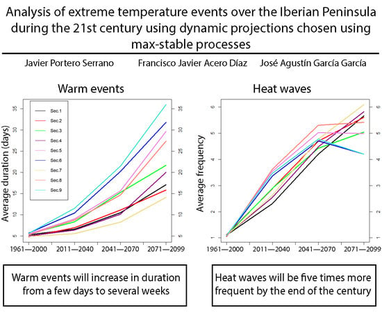
Analysis of Extreme Temperature Events over the Iberian Peninsula during the 21st Century Using Dynamic Climate Projections Chosen Using Max-Stable Processes

Abstract

Due to climate change, the Iberian Peninsula is suffering an increasing trend of extreme temperature events. The main objective of this study is to analyse this trends in frequency, duration and intensity of warm events and heat waves. The datasets used are 14 different regionalized dynamic climate projections. We choose the projections that present a spatial dependence similar to that of observed data. The spatial dependence is calculated by adjusting the data to max-stable processes. The observed data belong to the SPAIN02 grid for the period 1961–2000. We apply the Mann-Kendall test and the Theil-Sen estimator to calculate model trends in the future period (2011–2099). We have studied future extreme temperature events using two different definitions. One varying the threshold for each period and the other keeping it constant. The results show that the variability of maximum temperatures is decreasing for the western region of the Peninsula, while the Mediterranean area will see an increase in this variability. There will be an increase in the frequency of warm events for the southwestern corner of the Peninsula. Also, maximum temperatures will be higher in this area at the end of the century. However, in the Mediterranean region the warm events will last longer. Heat waves will be more frequent throughout the territory and more lasting in the Mediterranean area. We also found that studying extreme events using a varying threshold allows these events to be studied from the point of view of the variability of maximum temperatures, while if the study is carried out maintaining the threshold constant the results will be more direct.

1. Introduction

Climate change has become one of the greatest threats facing humanity. The global average temperature has risen 1.1 °C since the pre-industrial era and it is in a continuous increase [1]. In 2018, Spain and Portugal experienced their warmest summer since 2003 [2]. In addition, in 2003 the warmest summer since the early 1970s occurred [3]. The Iberian Peninsula (IP) is characterized by having an industrial base focused on the agricultural sector, being the fourth European country in crop production, and because of its biodiversity which is very important for tourism. Due to these reasons, the IP is especially vulnerable to the effects of climate change. In the last decades, there has been an increase in the aridity of the land, droughts, and the risk of fires [4]. Erosion and desertification, especially in the southeast of the IP, have reached a critical level, and continues expanding [5].

The emergence of several mega heat waves in recent years in different parts of Europe [6] and more recently in France, in addition to various studies [7,8,9], suggest that occurrences of such extreme temperature events will become more frequent in the next decades. This extreme temperature increase causes a great impact on the health of human beings and is directly related to cases of hospitalization and death when a certain temperature threshold is exceeded [1]. Because of the situation, a major economic and social impact is coming into being. The increase in temperatures and drought affects agriculture [2,10] and livestock [11]. It also causes changes in water resources [12] and extreme weather events [13]. In particular, extreme temperature events have been increasing not only in their frequency over the last two decades, but also in their duration and intensity [14,15].

The objective of this paper is to study the evolution of extreme temperature events over the IP during the 21st century. We also study trends in three characteristics of extreme temperature events: frequency, duration and intensity. In addition, we perform an analysis of the low percentiles of maximum temperatures. In this way we connect the results of extreme temperature events to changes in the amplitude of maximum temperatures. The previous hypotheses that we are using, comes from a previous study of extreme temperature events in a southwestern region of the IP [14]. The results of this study are related to warmer summers, longer and more intense extreme temperature events and fewer days with lower maximum temperatures. We expect similar results for the near future, although we assume that the increase in the characteristics of extreme temperature events will become more abrupt throughout the future period.

Extreme temperature events are more or less prolonged periods in which temperatures far exceed the most usual temperature range over a certain region. It is important to establish a correct definition of these events for two main reasons. The first reason is that a dramatic increase in temperatures is associated with short-term markers of mortality [16]. The second one is based on the fact that the study of heat waves is a good sign of the evolution of temperatures in a given region due to climate change [1]. Defining heat waves too rigidly would mean not considering certain extreme temperature events, which would signify a problem in studying their evolution over time and besides, the population would not be alerted to risks of this type of event, thus preventing proper precautions from being taken.

Studying the evolution of temperature extremes in a future period has been done before for different regions obtaining different results. Some of these previous results relate the evolution of mean temperatures more frequently to the occurrence of maximum temperatures [17]. Nevertheless, other studies suggest that the increase in maximum and minimum temperatures will be similar to changes in mean temperatures [18]. In previous works on temperatures it is common to analyze the evolution of temperatures by studying temperatures values, while for other variables such as precipitation, [19] it is usual to study their trends.

For this work we use data with the maximum daily temperature of the summer months (June, July and August) from fourteen regionalized dynamic projections. It is important to remark that the projections have a high resolution and a dynamical downscaling [20] in order to adjust to the peculiar orographic characteristics of the IP. These types of dynamic projections are widely applied to estimate future temperatures, rainfall, and wind extremes [21]. They are also used to predict climatic extremes [22] and future droughts [23].

We do not analyze the evolution of extreme temperature events with data from all climate projections. We must choose those whose behaviour resembles that presented by a dataset of observed temperature data. This dataset is the gridded dataset SPAIN02 [24]. The first comparison criterion analyzes the temperature distribution over the region for different established thresholds. This criterion ensures that the global climate projections have been correctly regionalized for the IP so that the data are adjusted to the orographic conditions of the region. All the projections used have been dynamically downscaled which gives us some confidence in the results obtained for future periods [25].

The second criterion is the comparison between the spatial dependencies of the models and the observed data. This is realised by calculating the extreme coefficient using max-stable processes. A max-stable process allows to find a unique stochastic model for different series of values, by introducing different continuous function series and fulfilling the condition of convergence. The max-stable processes are used as a modeling tool [26,27], however it is also a strong tool for comparison between extreme dataset [28]. Fitting climatological data to max-stable processes to calculate the spatial dependence of a model and using it as a comparison criterion is something new in the field of climatology. This is one of the key points of this work.

Furthermore, we study trends in the characteristics of extreme temperature events for the comparison period. This allows us to compare the trend behavior of the models with the one of the observed data. It also allows us to analyze the evolution of extreme temperature events during the comparison period and to study the change in their evolution during the future period.

The structure of the paper is as follows: The dataset we use are described in Section 2; the methodology that we use to analyze the data sets is described in Section 3; the results we achieve in the work are shown in Section 4 and discussed in Section 5; finally, we present the main conclusions in Section 6.

2. Dataset

The area of study is the IP, located in the southwest corner of the European continent (Figure 1). The IP covers the countries of Spain and Portugal, as well as the microstate of Andorra and the British Overseas Territory of Gibraltar. It is located in middle latitudes of the northern hemisphere, between the Atlantic Ocean and the Mediterranean Sea. The average elevation of the IP is 660 m, being surpassed in Europe only by Switzerland (1330 m). This is because most of the Iberian territory is constituted by an extensive plain, the Inner Plateau. In addition to this Central System, the IP has several peripheral mountain ranges such as the Pyrenees, the Cantabrian Mountains and the Baetic System. There are also two pronounced depressions, the valley of the Ebro to the northeast and the valley of the Guadalquivir to the southwest.

This peculiar topography causes the distribution of maximum temperatures to be very uneven over the territory. The altitude is the main factor affecting the temperature of the region. The warmest areas belong to the valleys in the south of the Peninsula, as well as to the Inner Plateau. The large mountain ranges, such as the Central System or the Pyrenees, present the areas with the lowest temperatures. The IP does not have a large enough surface area for the difference in latitude to significantly affect temperatures. The fact that the northern half of the region has lower temperatures than the southern half is related to the greater occurrence of mountain systems in this area. Due to these different characteristics that appear all over the territory, it is important to use dynamic regionalized projections with high resolution. Dynamic downscaling makes it possible to reduce the resolution of a model by introducing the global climate model into a regional numerical model that simulates local geographic and climatic conditions [29].

We used two datasets in this study.

Table 1. The 14 climate projections, their institution of origin, the climate models with which they have been developed and the average increase in maximum temperatures.

Acronym	Institute	General Circulation Model	Regional Climate Model	Equilibrium Climate Sensitivity (K)
C4I	Swedish Meteorological and Hydrological Institute (Sweden)	HadCM3Q16 [30]	RCA3.0 [31]	4.62 [32]
CNRM	Météo-France (France)	ARPEGE [33]	RM5.1 [34]	2 [35]
DMI	Danish Meteorological Institute (Denmark)	ARPEGE	HIRHAM5 [36]	2
		ECHAM5 [37]	HIRHAM5	3.65 [38]
ETHZ	Swiss Institute of Technology (Switzerland)	HadCM3Q0 [30]	CLM2.4.6 [39]	4.62
HC	Hadley Centre for Climate Prediction and Research (United Kingdom)	HadCM3Q0	HadRM3Q0 [40]	4.62
		HadCM3Q3 [30]	HadRM3Q3 [40]	4.62
		HadCM3Q16	HadRM3Q16 [40]	4.62
ICTP	The Abdus Salam International Centre for Theoretical Physics (Italy)	ECHAM5	REGCM3 [41]	3.65
KNMI	The Royal Netherlands Meteorological Institute (Netherlands)	ECHAM5	RACMO2.1 [42]	3.65
MPI	Max Planck Institute for Meteorology (Germany)	ECHAM5	REMO5.7 [43]	3.65
SMHI	Swedish Meteorological and Hydrological Institute (Sweden)	BCM [44]	RCA3.0	2 [44]
SMHI	Swedish Meteorological and Hydrological Institute (Sweden)	ECHAM5	RCA3.0	3.65
SMHI	Swedish Meteorological and Hydrological Institute (Sweden)	HadCM3Q3	RCA3.0	4.62

shows the 14 dynamic climate projections that have been used. They are a multi-model set of coupled simulations with the ERA-40 reanalysis as boundary conditions over the 20th century. This reanalysis makes it possible to reduce the variations in the models and, if the observations belong to a sufficiently long period, can correct the trends in the climate model. This makes the trends in the dynamic projections behave more appropriately to the observed data [45]. Models has been produced with the scenario A1B of aerosol and GHG forcing proposed by IPCC. This is a medium emission scenario that considers future development to correspond to a world with rapid economic growth based on the balanced use of all kinds of new and efficient energy sources and technologies. In addition to scenario A1B, a stabilization scenario to 450 ppm CO2 equivalent is used [46]. This A1B scenario assumes an annual growth rate in CO2 emissions of 1.1% in the 1990s, 0.5% in 2020, and 0.4% in 2050–2100 [47]. However, the growth in CO2 emissions between 2000 and 2009 was, on average, 3% per year [48]. If this difference between annual growth rates keeps increasing, the models based on this scenario would be underestimating the consequences resulting from future global warming.

We take them from the Spanish Meteorological Agency (AEMET). All of them belong to the European project ENSEMBLES [49]. They are global projections that have been regionalized for the IP with a grid width of 0.25° (Figure 2a). This dataset corresponds to daily maximum temperature data for the summer months between 1961 and 2000, as well as between 2011 and 2099. The temporality of the data series is divided into three periods: from 1961 to 2000 is considered a comparison period, from 2011 to 2040 a near future period, and from 2040 to 2099 a distant future period. The differences between periods are mainly related to the uncertainties in the temperature values of the climate projections, being able to separate the future in two different periods with different uncertainties, the first one until mid-term future and the second one from mid-term to long-term future [47] However, in this study we decide to divide the future period into three different sectors to emphasize the results for the first third of the century (near future period). The results of this period are of particular interest when planning short-term climate policies [50]. In this way, the future periods to be worked with will be 2011–2040, 2041–2070, 2071–2099. We use the comparison period (1961–2000) to compare the data from the climate projections with observed data (as will be seen below). Despite using fourteen dynamic projections, only those with a distribution and behaviour similar to the observed data are selected to study trends in future period.

The other dataset corresponds to the SPAIN02 grid (Figure 2b) for maximum temperature data in summer months. The SPAIN02 grid, with 0.1° of grid width, has been interpolated from observed data collected at 250 observatories distributed throughout the Spanish territory. We use these observed data to evaluate model simulations and limit the set of future projections to those of models capable of adequately capturing the temperature evolution observed in the past

3. Methodology

We use fourteen dynamic projections belonging to the ENSEMBLE project, but not all of them show similar behaviour to the data observed for the IP. Therefore, it is necessary to establish some comparison criteria with the observed data (SPAIN02) in order to filter the models. It is important to establish sufficiently strong comparison criteria to choose models with a similar behaviour to the observed data. However, excessively rigid criteria for comparison may lead to discard too many projections. Uncertainty in future climate change estimates arises from three factors [51]. The first one is the difference between climate models. The uncertainty of this factor is minimized by choosing models with similar spatial dependence [28]. The second factor is the difference between forcing scenarios (Table 1). The third factor is the uncertainty due to internal variability of climate variables. This uncertainty can be reduced by using very large dataset sizes, however, for surface temperature at mid-latitudes at least 3–12 datasets are needed [52]. So studying future trends using few climate projections may lead to an increase in the uncertainty of long-term results. Individual simulations have uncertainty associated with internal variability [53]. These anomalies caused to reach values of 1.5 °C for return periods of 20 years for average European summer temperatures. These increase for the southern regions of the continent, where the IP is located [54]. Since in this work we use maximum temperatures instead of average temperatures we should expect a higher uncertainty.

The first characteristic we analyze is that the spatial distribution throughout the entire territory is the same as for the observed data. With this, we ensure that the models resemble the stationary conditions of the temperatures.

The second comparison criterion is to study the spatial behavior of the data. This is the fundamental criterion for comparison. The temperatures observed in a region are not independent of each other, i.e., the evolution of temperatures in two nearby locations should be similar. On the other hand, if the observation stations are far apart, the evolution of the temperatures will be independent of each other. This dependence or independence is also related to the orographic conditions of the terrain, among other aspects. For this reason, we study the spatial dependence of the dynamic projections and the observed data.

3.1. Definition of Extreme Temperature Events

Many definitions of heat waves can be found [55]. They all consider a heat wave to be a period of various days in which the maximum temperature exceeds a certain threshold. For this study, we considered a period of two consecutive days above the threshold, taking the 95th percentile of the summer maximum temperature as threshold for heat waves, and the 75th percentile as threshold for warm events [14]. For heat waves, this threshold reaches values of more than 40 °C in the warmest areas of the IP (the southwest and the valleys of the Ebro and Guadalquivir rivers) and around 25 °C in the more temperate zones (mountain ranges in the northern half of Spain).

Having established a definition for extreme temperature events, we define three characteristics of these events: frequency, duration, and intensity (Figure 3). We consider frequency as the number of times extreme temperature events occur during the summer months of a certain year, duration as the number of consecutive days in which temperatures have exceeded a certain threshold, and intensity as the difference in temperature between the maximum temperature reached in an extreme temperature event and the threshold that defines that event.

We shall establish a nomenclature to distinguish three temperature ranges. Those maximum temperatures that exceed the heat wave threshold (95th percentile) are denoted T95, those that exceed the warm event threshold (75th percentile) but not the heat wave threshold are denoted T75, and, finally, those that are below the 25th percentile are denoted T25. This low temperature percentile (T25) is chosen in order to analyze the role of the variance in the evolution of extremes as shown in previous works [14,56] in which low values of the maximum temperatures showed a greater increase than high values leading to a decrease in variance.

The analysis of the characteristics of extreme temperature events is been carried out from two different points of view. The first (varying threshold) involves choosing a different threshold for the four study periods being that threshold the corresponding percentile for each period. The second (constant threshold) involves choosing un unique threshold, the corresponding to the comparison period 1961–2000, in order to study the changes in the characteristics of the events in future climate against the characteristics in the past. It is important to evaluate the relevance in the approach of the results for both studies, since establishing a more or less rigorous definition for extreme temperature events can make the information easier to understand for politicians and non-experts. This may change the way climate impacts are assessed for the future.

3.2. Identification of Trends

We analyze extreme temperature events for their characteristic magnitudes (frequency, duration and intensity) for each year. We calculate the trend for each of these results using the Theil-Sen estimator [57] for the value of the trend and the Mann-Kendall test [58] for the significance of that trend [59]. We use the Theil-Sen estimator because is better than non-robust linear regression for long-term series because it is less sensitive to outliers than least-squares linear regressions. The Kendall test is used as a complement to the Theil-Sen estimator to calculate the significance of the trends [60].

In order to analyse the results more easily, we divide the study region, the IP, into different sectors with similar geographical characteristics. Figure 4 shows the nine sectors.

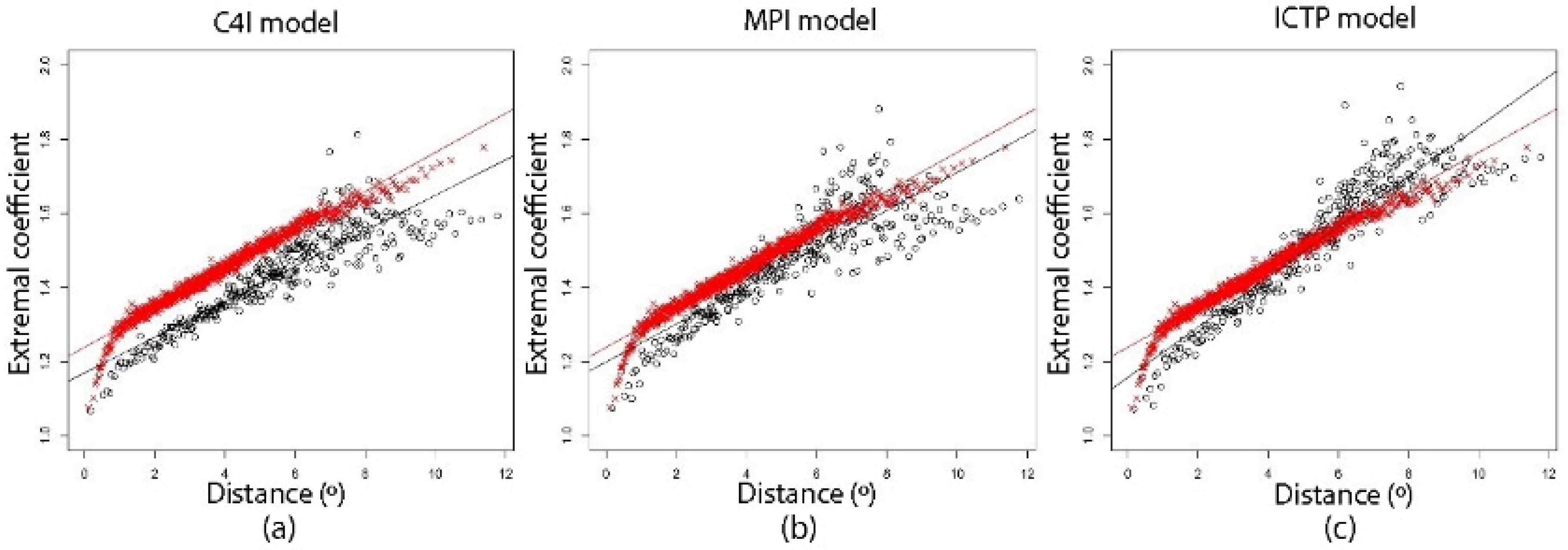
3.3. Spatial Dependence

It is important to choose dynamic projections whose simulated data resemble the observed data. This is done by comparing the simulated data with the actual data using different criteria during a period in which the two coexist. In this work, this period is from 1961 to 2000.

As a comparison criterion, we compare the spatial dependence of the datasets. For this, we calculate the extremal coefficient from the fit of the data to a max-stable spatial process. A stochastic process $\left\{Z\left(r\right):r\in ℝ\right\}$ is defined as a max-stable process if there exist successions of continuous functions $\left\{a_n\left(r\right)>0:r\in ℝ, n\ge 1\right\}$ and $\left\{b_n\left(r\right)\in ℝ:r\in ℝ, n\ge 1\right\}$ such that, for all $n\ge 1$:

$$\left\{\frac{{\displaystyle \underset{i=1,\dots ,n}{\max }}{Z}_i\left(r\right)-b_n\left(r\right)}{a_n\left(r\right)}: r\in ℝ\right\}\stackrel{\scriptscriptstyle\mathrm{def}}{=}\left\{Z\left(r\right):r\in ℝ\right\}$$

(1)

where $\left\{Z_i\left(r\right): r\in ℝ, i\ge 1\right\}$ is a succession of independent replicas of $\left\{Z\left(r\right): r\in ℝ\right\}$ [61]. It seems appropriate to use max-stable processes for this study since our dataset can be divided into subsets with the same dimensions separating stations for each year. There are various representations of max-stable processes [62]. For this work, we use the Schlater approach, which is the one that best fits temperature data [63]. This rewrites the max-stables process as:

$$Z\left(x\right)=\stackrel{\scriptscriptstyle\mathrm{def}}{=}{\displaystyle \underset{i\ge 1}{\max }}{\zeta }_i{Y}_i$$

(2)

where $\left\{{\zeta }_i: i\ge 1\right\}$ are points of a Poisson process at $\left(0,\infty \right)$ and $Y_1,Y_2,\dots$ are independent replicas of a stochastic process $\left\{Y\left(x\right): x\in X\right\}$. This results in a distribution:

$$P\left(Z\left(r\right)\le z_1, Z\left(r+h\right)\le z_2\right)=exp\left\{-\frac{1}{2}\left(\frac{1}{z_1}+\frac{1}{z_2}\right)\left(1+\sqrt{1-2\left(\rho \left(h\right)+1\right)\frac{z_1{z}_2}{{\left(z_1+z_2\right)}^2}}\right)\right\}$$

(3)

where $\rho \left(h\right)$ is the correlation function.

Also, we must define the extremal coefficient function. This is used to measure the dependence between the extremes of two random vectors $\left(X,Y\right)$ with common marginal distribution, $F\left(r\right)$. The extremal coefficient, $\theta$, is defined by the following expression:

$$P\left(\max (X,Y\right)\le x)=F^{\theta }\left(x\right)$$

(4)

The extremal coefficient can take values within the range $\left[1,2\right]$, where $\theta =1$ is considered perfect dependence between maxima and $\theta =2$ absolute independence. Applied to max-stable processes, the extremal coefficient function expressed as [64]:

$$P\left(\max \left(Z\left(r\right),Z\left(r+h\right)\right)\le z\right)=e^{\raisebox{1ex}{$-\theta \left(h\right)$}\!\left/ \!\raisebox{-1ex}{$z$}\right.}$$

(5)

where $Z\left(r\right)$ is a max-stable process, $\theta \left(h\right)$ is the extremal coefficient function and $h$ is the distance that separates different maxima. In the present case, $h$ will be the distance between different points of the dataset grid.

We also need to define a basic tool to measure spatial dependence, the F-madogram. With $Z\left(x\right)$ being a stationary process, in our case a max-stable process, the F-madogram is defined as:

$$\nu \left(h\right)=\frac{1}{2}E\left[\left|F\left(Z\left(x+h\right)-Z\left(x\right)\right)\right|\right]$$

(6)

where $F\left(x\right)$ is the cumulative distribution function of $Z\left(r\right)$. The relationship between the F-madogram and the extremal coefficient is [65]:

$$\theta \left(h\right)=\frac{1+2\nu \left(h\right)}{1-2\nu \left(h\right)}$$

(7)

This allows us to have an extremal coefficient function for each pair of grid points, i.e., a spatial dependence function for the distances that separate the coordinates of the region.

4. Results

4.1. Comparison Period

4.1.1. Threshold Distribution

Figure 5 shows the percentile distribution of the SPAIN02 grid dataset. This distribution is related to the orographic characteristics of the region. The dynamic projections have to show a distribution similar to this one. Low values are located in the Pyrenees, the Cantabrian Coast, and the Central, Iberian, and Baetic Systems. High values are located in the Ebro and Guadalquivir river valleys.

The dynamic projections that present this distribution are C4I-RCA3.0-HadCM3Q16 (C4I), CNRM-RM5.1-ARPEGE (CNRM), DMI-HIRHAM5-ECHAM5-r3 (DMI), ICTP-REGCM3-ECHAM5-r3 (ICTP), KNMI-RACMO2.1-ECHAM5-r3 (KNMI), MPI-REMO5.7-ECHAM5-r3 (MPI), SMHI-RCA3.0-ECHAM5-r3 (SMHI). They can be seen in Figure 6. For simplicity, from now on we call these projections only by the name of the institution that developed them (in parentheses) rather than by their full nomenclature. We need to emphasize that, although the temperature values are different from those of the SPAIN02, what is important is that the distribution of the maxima and minima is correct.

4.1.2. Spatial Dependence

The key criterion for the comparison between projections and the observed data is the calculation of the spatial dependence. The plots should be read as follows. The abscissae represent the geographic separation (in degrees) between the points at which the spatial dependence is to be estimated. For this work these are the grid points. The ordinates represent the extremal coefficients, i.e., the spatial dependence between points, with 1 being perfect dependence and 2 absolute independence. It can be seen in the SPAIN02 plots (red points in plots of Figure 6) that the relationship between the temperature variations becomes more independent as the points are farther apart, whereas the closer the points are, the more dependent they are. This is logical since the temperatures of nearby points are directly related, and events that cause changes in one will also cause them in others.

Table 2. Linear regression coefficients of the extremal coefficients.

Model	Slope	Intercept	Slope Error (%)	Intercept Error (%)
C4I	0.050	1.169	5.109	5.581
CNMR	0.062	1.180	18.130	4.685
DMI	0.068	1.157	28.641	6.582
ICTP	0.046	1.228	12.142	0.890
KNMI	0.061	1.137	16.358	8.191
MPI	0.051	1.199	2.821	3.196
SMHI	0.059	1.161	12.847	6.259
SPAIN02	0.053	1.239	0.000	0.000

shows the adjustment coefficients of the extremal coefficients by linear regression (Figure 7). The only models with a similar slope (slope error < 10%) to the observed data are the C4I and MPI models. The other models have a much steeper slope than the observed data, so the simulated data tend to be more independent (Figure 7c).

Analyzing intercept errors, it is common that intercept points are smaller than observed data, since model data is generated from boundary conditions, which makes them more dependent on nearby points [47]. Therefore, this does not provide much, the key point is that the behaviour at different distances is similar. The only models that achieve this are the C4I and the MPI.

4.1.3. Percentile Trend

Figure 8 shows that 95th percentile show similar trends for the models and the observed data. These are significantly positive and are accentuated when approaching the Mediterranean coast (to the east). To allow a better interpretation of the spatial behaviour of the results, the trends are spatially interpolated by the Kriging procedure. This interpolation is shown in color at the back of the figure.

Figure 9 shows how the model trends resemble the trend of the observed data. We should exclude sectors 4 and 7 from the comparison as for the observed dataset Portugal was not included.

The study of the trends for the 75th percentile gives identical results to those of the 95th percentile. The sectors with the highest trend are sectors 5 and 6, the central and Mediterranean region of the Peninsula. Similar results are observed for the 25th percentile. This implies that for the comparison period (1961–2000), T95, T75, and T25 have been increasing uniformly, which implies warmer temperatures but maintaining its distribution.

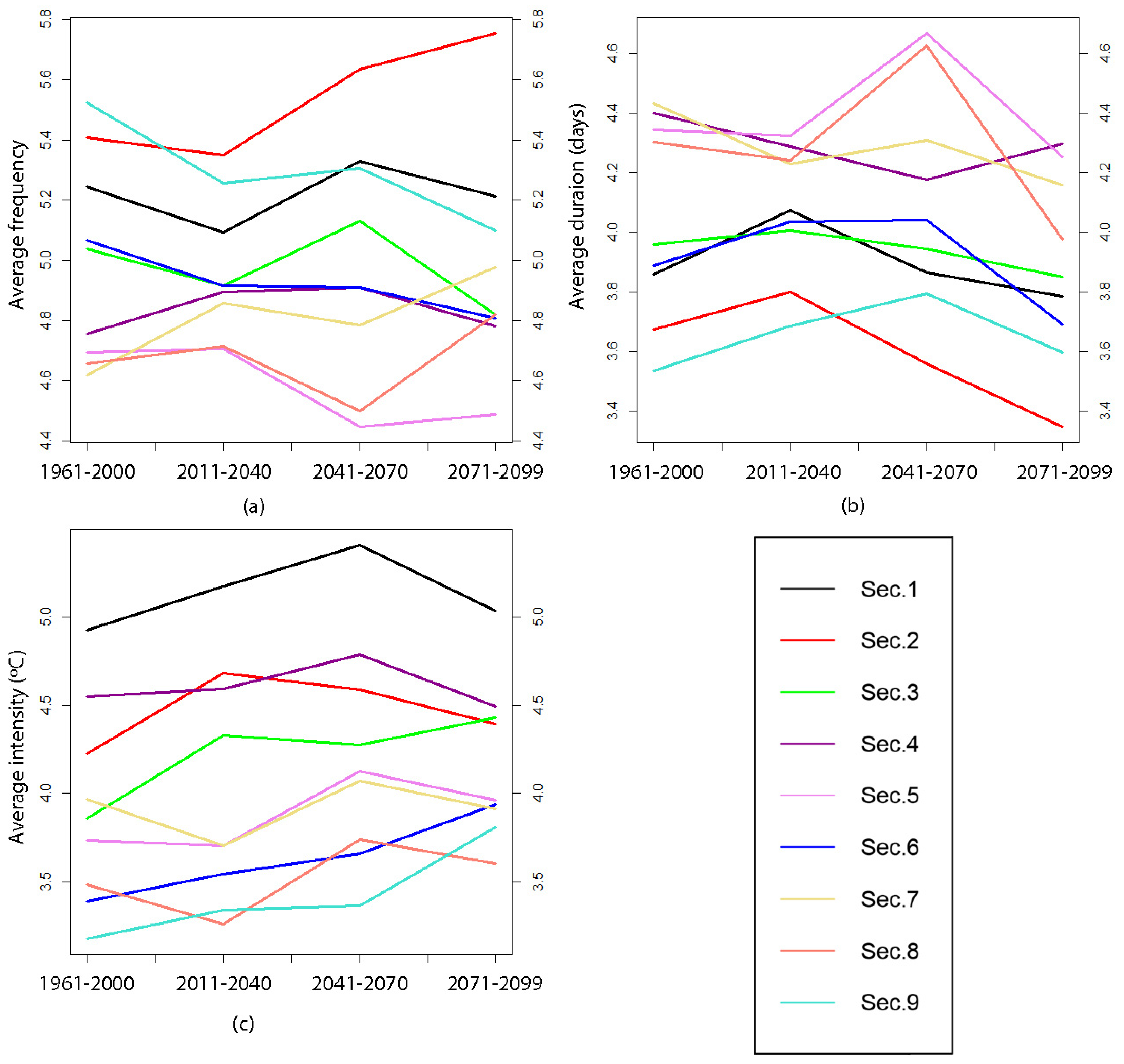
4.1.4. Trends in Warm Events Characteristics

Analysing the characteristics of warm events, for both the C4I and the MPI models it can be observed that their duration presents a mostly positive and significant trend, with an increase from west to east over the Spanish territory. The intensity and frequency of warm events show no tendency during the comparison period. This implies that, over the four decades covered by this period, extreme temperature events have become neither more intense nor more frequent but have lasted longer.

Again, the most affected sectors by the increase in the trend are 5 and 6 (Figure 10). This is in accordance with the results obtained for the percentile trends. The maximum temperatures have been increasing uniformly, so that the temperatures are increasing above the 75th percentile.

4.1.5. Trends in Heat Waves Characteristics

Studying the trends for heat waves, it has been found that the three characteristics (frequency, duration and intensity) do not present significant trends in any sector of the region. Therefore, it is considered that the characteristics of heat waves during the comparison period have remained stable.

4.2. Future Period

Once the two models (C4I and MPI) have been chosen, we study the distribution of thresholds and trends of percentiles and extreme temperature events for those two models during the future period. This period covers from 2011 to 2099, using three different periods: 2011–2040, 2041–2070, and 2071–2099.

4.2.1. Threshold Distribution

Figure 11 shows the spatial distribution of T95 for the three sub-periods considered along the 21st century. The areas showing maximum and minimum temperatures remain constant for all the sub-periods. However, one can see an increase in temperatures, which reach values above 50 °C by the end of the 21st century.

4.2.2. Percentile Trend

Analysing the trends in the 95th percentile, one finds disparate results in both models for the first third of the 21st century. The C4I model presents significant positive trends which are evenly distributed throughout the territory, increasing in value in the regions closest to the Mediterranean coast. These trends increase dramatically during the second third of the future period. The MPI model presents disparate results for the first third. A significant positive trend appears in the central part of the territory, while in the periphery there is no significance. The value of this trend is very small. However, for the following two periods, the results resemble those of the C4I model, with the trends being similar in magnitude.

Looking at Figure 12, this higher trend can be seen in sectors 6, 8 and 9. However, the regions with the highest T95 would be sectors 7 and 8, reaching an average T95 of more than 46 °C for the last third of the century. It can also be seen that temperatures increase their trend from the middle of the century onwards.

For the 75th and 25th percentiles, the results are the same as for the 95th percentile, although the value of the 25th percentile trend increases after half a century, with this increase being greater in T25 than in T95 and T75.

Figure 13 shows these results for different locations, one for each sector. Temperatures for the first third of the century rarely exceed the 95th percentile, while from the middle of the century onwards they increasingly easily exceed that threshold.

By analyzing

Table 3. Average slope of the regression of T95 and T25 for each sector and the three future periods.

Sectors	Slope T95	Slope T25
Sector 1	0.08323	0.08748
Sector 2	0.07970	0.07723
Sector 3	0.08193	0.08053
Sector 4	0.06999	0.07936
Sector 5	0.07386	0.09556
Sector 6	0.09350	0.07165
Sector 7	0.05913	0.06377
Sector 8	0.07821	0.07158
Sector 9	0.08303	0.07200

, the IP can be divided into two regions with similar characteristics. The western half, including the central zone (sectors 1, 4, 5 and 7) presents a T25 with a greater slope than T95, which implies that the variability of maximum temperatures in this region is decreasing. On the other hand, sectors 2, 3, 6, 8 and 9, corresponding to the Mediterranean area of the IP (except sector 2) present a T25 with a lower tendency than T95, which means that the variability of maximum temperatures will increase throughout the century.

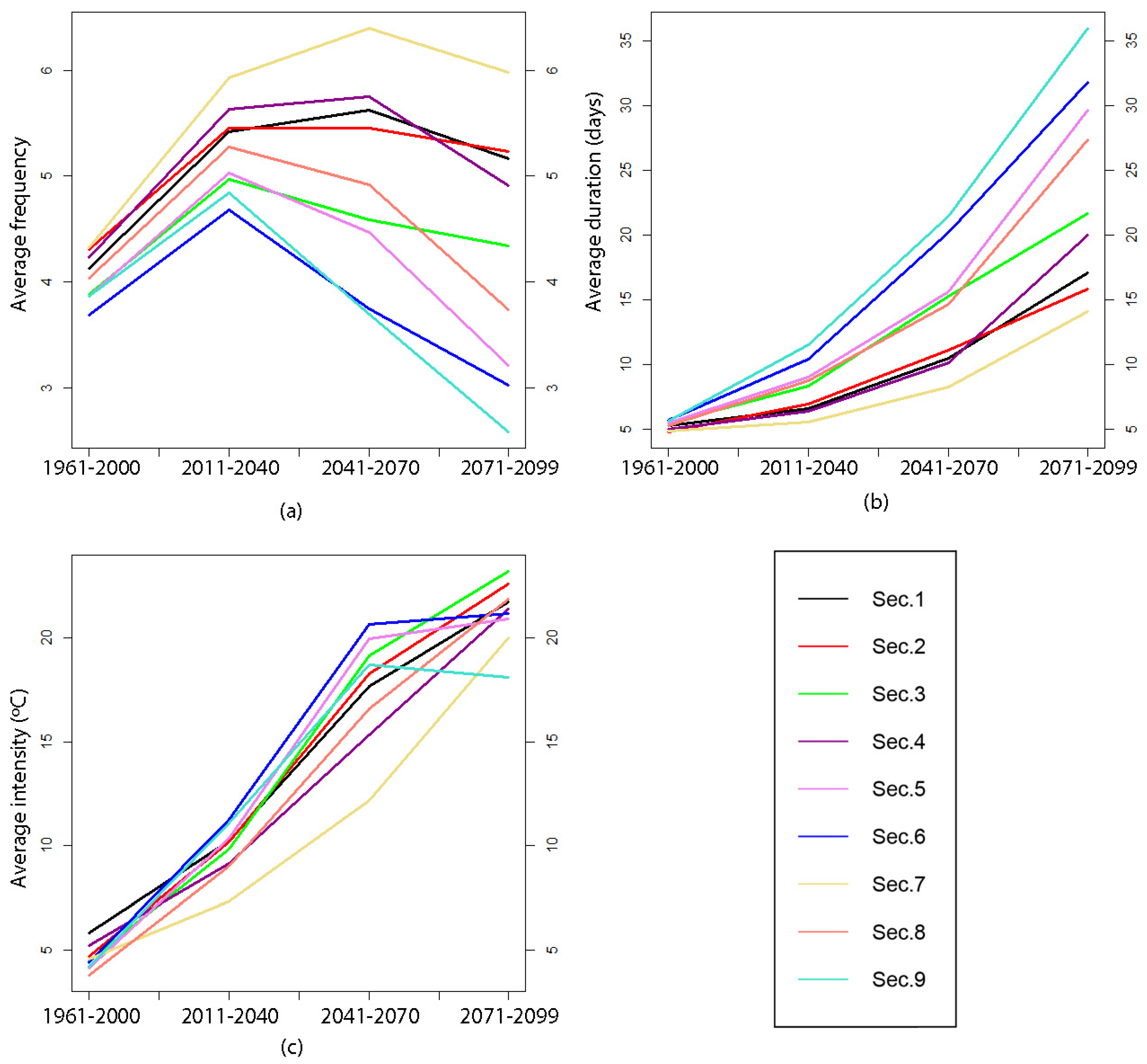
4.2.3. Trend in Future Warm Events Characteristics

The results for the trends in warm events characteristics considering a varying threshold lead to a similar spatial distribution for those trends for the two selected models. Figure 14 shows the spatial distribution of the trend in warm event frequency for the C4I model. Figures for the remaining characteristics have been omitted remarking in the text the main results. The duration of warm events shows a positive trend, mostly significant, that occurs irregularly throughout the entire Iberian territory. This trend is accentuated for the second third of the century in the central zone and the northwestern corner and remains constant over the last third of the century.

The frequency and the intensity of warm events have the same distribution during this period. In the first third of the century, there is an irregular distribution similar to that presented by the durations. As time passes, the trends increase dramatically in the eastern half of the Peninsula. This is consistent with the results obtained for the comparison period, in which the frequency and intensity of warm events remained unchanged. After the first third of the 21st century, temperatures will exceed the 75th percentile with greater frequency and intensity. With respect to duration, the trend already noted in the comparison period increases even further in the future period, with ever longer-lasting warm events appearing as time goes on.

Figure 15 shows the average characteristics of the warm events considering varying threshold for all the sub-periods considered. The northern sectors of the Peninsula (1, 2 and 3) suffer most frequently from warm events. The warm events with the longest average duration appear in the southwest quadrant (sectors 4, 5, 7 and 8) and the most intense warm events appear in the northwest region (sectors 1, 2 and 4).

The results with constant threshold for warm events trends (figures are also omitted) for the whole future period are as follows. The frequency does not show significant trends in any part of the region over the whole future period. This occurs because as the temperature increases in the future most days will be above the 75th percentile resulting in a decrease in frequency and an increase in duration. The duration of the warm events shows significant positive trends throughout the territory, which is increasing throughout the whole future period, especially in the extreme south-east of the Peninsula and the eastern Cantabrian coast. Trends in the intensity for warm events show a similar behaviour than the trend in duration increasing from 2011–2040 to 2041–2070 but remain constant from this last period to 2071–2099.

Figure 16 shows the evolution of the warm events characteristics considering as constant threshold the corresponding of the comparison period for the rest of future periods. It can be seen how the frequency of warm events decreases throughout the future period. The regions with the highest frequency of these events are the Cantabrian coast and the Atlantic coast of the Peninsula (sectors 1, 2, 4 and 7). It can be seen that the duration increases exponentially for the whole territory, being greater for the southeast quadrant of the IP (sectors 5, 6, 8 and 9). The intensity increases uniformly until the second third of the 21st century. From this period onwards, the average intensity of sectors 5, 6 and 9 remains uniform until the end of the century, while the rest of the sectors continue to increase to the same extent as during the previous period.

4.2.4. Trends in Future Heat Waves Characteristics

The results for the trend in heat waves characteristics considering a varying threshold are disparate between the two models. Again, figures for the trend characteristics have been omitted, but main results are highlighted in this subsection. The C4I model presents positive, mostly significant, trends for duration that are irregularly distributed throughout the Peninsula, especially in Portugal. This situation remains stable throughout the rest of the 21st century. For frequency and intensity, the same irregular distribution of trends can be observed, but with much lower values.

For the MPI model, an almost null trend map is observed for the three characteristics of heat waves during the first third of the century. From the second third of the century onwards, significant positive trends begin to appear in the northwestern quadrant of the region, which are accentuated during the last part of the century. Trend values for frequency and intensity are very small compared to those for duration and compared to those of the C4I.

These results indicate that the frequency of heat waves increases progressively during the 21st century, with the 95th percentile being surpassed ever more often. Since there is no agreement between the two models in their results for the duration and intensity of heat waves, and since the values of the trends are very low, conclusive results cannot be presented for these two magnitudes.

However, considering the 95th percentile of the comparison period as constant threshold for the future periods the results are different. Figure 17 shows that trends in heat wave characteristics using varying threshold (Figure 17a) are not meaningful compared to constant threshold (Figure 17b). There is an increase in frequency that persists uniformly until the end of the second third of the 21st century, and is unevenly distributed throughout the territory. During the last third, this increase disappears giving rise to a decrease in the southeast quadrant of the region. For duration and intensity of heat waves the results are similar, a large increase throughout the territory. This increase is becoming greater and greater throughout the century and is slightly stronger in the Mediterranean area of the Peninsula (sectors 3, 6 and 9).

5. Discussion

We divided the results into two blocks. The first block corresponds to the comparison period and the second to the future period. The results for the comparison period are related to the comparison criteria when choosing the models for this work. The first criterion for comparison we use is to compare the distribution of temperatures across the region. Of the 14 dynamic projections, seven fit the orographic distribution of the IP. These are the C4I, CNMR, DMI, ICTP, KNMI, MPI and SMHI models.

The second criterion for comparison has been to study the spatial dependence of the projections by calculating the extremal coefficient. This criterion has been the key to choose the projections because it gives the study an extra layer of depth. Of the seven dynamic projections that passed the first criterion, only two have met this criterion. This implies a number of problems such as working with only two individual long-term simulations does not ensure that the results are not affected by the effects of internal variability [66]. There are several possible solutions to this problem. Within the climate domain, it can be solved by using average maximum temperatures over larger areas or by removing the noise generated by internal variability [53]. Larger scale simulation sets [66] can also be used. However, that solution can make us lose focus about studying extreme temperature events by differentiating the distinct different regions of the IP. Since the criterion that leaves us with only two dynamic projections has been the calculation of spatial dependence, an improvement to relax this criterion would be to improve the fit of the data to the max-stable process using different approaches made by different algorithms [67]. A temporal variable can also be added to the max-stable process along with the spatial variable [68]. This can make the data adjustable in the case of using longer time periods and can be a good point to develop in further work.

The two models chosen were the C4I model and the MPI model. Both of them, use different global and regional climate models. The results for both models are very similar, however it can be observed that in the calculation of trends the same distributions can be seen for the C4I and MPI models, but the values of the trends are uniformly lower for the MPI model. This is caused by the f the equilibrium climate sensitivity (Table 1) that is greater for the C4I model than for the MPI model.

We also analyzed the evolution of T95, T75 and T25, and the characteristics of extreme temperature events for the comparison period. The results for the thresholds indicate that during this period T95 shows a significant positive trend for the whole territory. This trend is increasing in the Mediterranean sectors of the Peninsula. T75 and T25 present similar trends. Thus, maximum temperatures increased uniformly during the period 1961–2000. Furthermore, these trends also appear in the observed data, which gives us confidence in the choice of these two models.

For the characteristics of warm events the results are as follows: The intensity and duration of the warm events show no trend for the comparison period. However, the frequency of warm events does show a significant positive trend. This increase is greater in the central area of the Peninsula and in the Mediterranean coast. The trend analysis for heat waves during the comparison period does not show any significant trend. This implies that the characteristics of heat waves have not evolved during the period 1961–2000.

The results for the future period differ from those of the comparison period. The spatial distribution of the trends in T95, T75 and T25 suggest a positive trend in these percentiles throughout the 21st century for the entire IP. However, if we compare the evolution of T95 and T25, these two percentiles do not increase uniformly throughout the region. T25 increases faster than T95 on the Atlantic coast of the Peninsula, which includes the entire Portugal and the most western regions of Spain. This implies that the variability of maximum temperatures decreases in accordance with previous works [14,54]. On the other hand, in the Mediterranean regions of the Peninsula the maximum temperatures increase their variability. These results would be in agreement with previous studies which have been carried out on the southwest region of Spain [14], as well as with other studies that connect the increase of maximum temperatures in a non-uniform way [17]. Comparing the evolution of these thresholds during the comparison period with the trends for the future period are much higher. This implies a much more abrupt increase in maximum temperatures.

We have studied extreme temperature events from two different points of view. The first one consists of varying the threshold of these events for each study period. This methodology is more in accordance with the definition of extreme temperature events [53]. The second approaches the study by keeping the threshold constant, which is the threshold of the comparison period, in order to analyze future changes in extreme events characteristics.

For warm events, the results for varying thresholds show only a positive trend in duration in the central and northwestern area of the Peninsula, as well as a positive trend in frequency for the eastern half of the region. Both trends increase during the first half of the century and remain stable for the second half. But the results differ if the constant threshold is considered. The frequency of warm events does not show significant trends over the entire future period, but the duration and intensity have uniform positive trends for all the region. In the case of duration, this trend increases throughout the century, while the intensity of warm events remains stable from the second half onwards for the southern part of the Mediterranean coast. This decrease in frequency and increase in duration of warm events means that from 2041 onwards, summer maximum temperatures over the IP will be characterized by temperatures over the 75th percentile of the registered in the comparison period.

Heat waves also present distinct results for the two different thresholds. By keeping the threshold constant, the frequency of heat waves presents a uniform positive trend for the whole region. This trend remains constant until the end of the second third of the century and becomes negative during the end of the century for the southwestern corner of the region. The duration and intensity present positive trends over the whole territory. These trends increase during the entire future period, with a higher increase in the Mediterranean coast of Spain. Positive trends for the duration of heat waves appears at the moment of studying the trends with varying threshold, however, this trend is insignificant compared to the trend in duration for the constant threshold. There is no consistent trend in either frequency or intensity.

Figure 17 shows the heat wave characteristics using both, a varying threshold for each study period (left panels) and the heat wave threshold for 1961–2000 as constant for future periods (right panels). The results are different, there are no changes in the characteristics for a varying threshold but they increase remarkably if it is used a constant threshold. Therefore, future heatwaves will be much more intense, frequent and long-lasting than the registered in 1961–2000.

Finally, analyzing the evolution of extreme temperature events for the different sectors of the region, sectors 7 and 8 reach the highest temperature values. Sectors 5, 6 and 9 reach maximum temperatures slightly lower than these. These sectors correspond to the southern half of the IP. The maximum temperatures increase a lot during the whole 21st century, being this increase of more than 5 °C for the whole Peninsula.

Warm events increase in frequency at the beginning of the 21st century, but peak at the end of the first third. From this time until the end of the future period the frequency decreases. However, the duration of these events increases exponentially, from an average duration of 5 days for the comparison period to an average duration of more than 20 days by the end of the century. The intensity also increases over the future period. This increase rises from the middle of the century onwards. At the end of the century we can distinguish two regions with different behaviours. Regions 6, 7 and 9 (southeast Spain) keep the intensity of warm events constant, while in the rest of the sectors the intensity continues to increase. The average intensity at the end of the century exceeds 21 °C. The southwestern sectors have higher temperature peaks and greater variability, so the duration increases but not the intensity. The other sectors have less variability of peak temperatures, so the intensity continues to increase at the end of the century. The behaviour of these three variables is explained by the enormous increase in maximum temperatures above the constant threshold. This transforms warm events from many warm events per year of short duration during the near future period to few events per year of very long duration and high intensity during the last decades of the 21st century.

For heat waves, the frequency will increase uniformly throughout the century. At the end of the century the frequency of heat waves is five times higher than during the comparison period. The duration also increases throughout the territory. However, this increase is more pronounced in sectors 3, 5, 6, 8 and 9 (Mediterranean coast and center of the peninsula). This behaviour can also be observed in the intensity of heat waves. This is in accordance with the previously mentioned change in the variability of the maximum temperatures that the different regions of the Peninsula will suffer. This increased variability also appears in other parts of Europe [69,70,71].

6. Conclusions

The first stage of this work is to consider different dynamic projections that can be used to analyse the evolution of temperatures in a future period (2011–2099). This was achieved by comparing the temperature data of the models and of extreme temperature events with the observed maximum temperature data for summer months between 1961 and 2000. These observed data come from the SPAIN02 grid of interpolated temperature data registered at 250 stations distributed throughout Spain.

There are two criteria for choosing climate projections that resemble their behaviour to the observed data. First, to study their spatial distribution for three chosen temperature thresholds (T95, T75 and T25). The second criterion is to study the spatial dependence of the models and the observed data by fitting them to a max-stable process. With this criterion of comparison, the are only two models that present a similar behaviour the C4I model and the MPI model.

The results for the evolution of maximum temperatures for the 21st century show a pessimistic outlook. T95 increases over the whole period in the whole IP. This increase becomes more pronounced from the middle of the century onwards, with temperatures reaching more than 45 °C in the southwest corner. Two regions can be distinguished with different amplitude behaviour of the maximum temperatures. The western half of the Peninsula shows a decrease in amplitude, while the Mediterranean half shows an increase in amplitude. This implies that the western half of the Peninsula will have a higher increase in its maximum temperatures with less variability.

With respect to extreme temperature events, we study them using two different points of view. With the variable threshold, the duration of warm events increases. This increase is accentuated from the second third of the century. For the frequency and intensity of warm events, a trend appears during the second third of the century and increases by the end of the period. Heat waves show a positive trend for their duration.

Results using the constant threshold show a very abrupt increase in the duration and intensity of warm events. This trend is increasing over the course of the century. However, the frequency does not show a trend throughout the century. For heat waves, the frequency presents a positive trend that remains constant throughout the century. The duration and intensity presents similar trends to those of warm events.

The difference between results appears due to the use of the varying threshold presents the trends of T95 and T25 in relation to the average maximum temperatures during the concurrent period. Using this threshold is more useful to studying changes in higher maximum temperatures compared to changes in moderate or lower maximum temperatures.

On the other hand, using the constant threshold is easier to appreciate the absolute change in the characteristics of extreme temperature events. This allows a simpler reading in order to relate it to the effects of climate change, so this is considered a more suitable approach to show results to politicians or non-experts in general.

The effect of extreme temperature events for the different areas of the IP are the following.It can be observed that the southwestern corner of the Peninsula (Beja and Faro, in Portugal, and southern Extremadura and western Andalusia, in Spain) will reach the highest temperatures, often exceeding temperatures of over 45 °C at the end of the 21st century. Warm events will also be more frequent in this region, although it is in the southeast corner of the Peninsula (southern Valencia, Murcia, eastern Andalusia and Castile-La Mancha) where these events will last more. Overall, the average duration of warm events for the entire region increases from 5 days (comparison period) to almost 24 days (2071-2099). As for heat waves, they will be almost as frequent throughout the territory, although they will be more lasting and more frequent along the entire Mediterranean coast.

References

1. IPCC. Global Warming of 1.5 °C. An IPCC Special Report on the Impacts of Global Warming of 1.5 °C above Pre-Industrial Levels and Related Global Greenhouse Gas Emission Pathways, in the Context of Strengthening the Global Response to the Threat of Climate Change, Sustainable Development, and Efforts to Eradicate Poverty; Masson-Delmotte, V., Zhai, P., Pörtner, H.-O., Roberts, D., Skea, J., Shukla, P.R., Pirani, A., Moufouma-Okia, W., Péan, C., Pidcock, R., et al., Eds.; IPCC: Geneva, Switzerland, 2018. [Google Scholar]
2. Mínguez, M.I. Agriculture in Spain and the Climate Change Issue; Research Center for the Management of Agricultural and Environmental Risks of the Technical University of Madrid (CEIGRAM): Madrid, Spain, 2016. [Google Scholar]
3. Brunet, M.; Jones, P.D.; Sigró, J.; Saladié, O.; Aguilar, E.; Moberg, A.; Della-Marta, P.M.; Lister, D.; Walther, A.; López, D. Temporal and spatial temperature variability and change over Spain during 1850–2005. J. Geophys. Res. 2007, 112, D12117. [Google Scholar] [CrossRef] [Green Version]
4. Piñol, J.; Terradas, J.; Lloret, F. Climate Warming, Wildlife Hazard, and Wildfire Occurrence in Coastal Eastern Spain. Clim. Chang. 1998, 38, 345–357. [Google Scholar] [CrossRef]
5. Martínez-Fernández, J.; Esteve, M.A. A critical view of the desertification debate in southeastern Spain. Land Degrad. Dev. 2005, 16, 529–539. [Google Scholar] [CrossRef]
6. Fischer, E.M. Autopsy of two mega-heatwaves. Nat. Geosci. 2014, 7, 332–333. [Google Scholar] [CrossRef]
7. Bador, M.; Terray, L.; Boé, J.; Somot, S.; Alias, A.; Gibelin, A.; Dubuisson, B. Future summer mega-heatwave and record-breaking temperatures in a warmer France climate. Environ. Res. Lett. 2017, 12, 074025. [Google Scholar] [CrossRef] [Green Version]
8. Meehl, G.A.; Tebaldi, C. More intense, more frequent, and more longer lasting heat waves in the 21st Century. Science 2004, 305, 994–997. [Google Scholar] [CrossRef] [Green Version]
9. Guerreiro, S.B.; Dawson, R.J.; Kilsby, C.; Lewis, E.; Ford, A. Future heat-waves, droughts and floods in 571 European cities. Environ. Res. Lett. 2018, 13, 034009. [Google Scholar] [CrossRef]
10. Olesen, J.E.; Bindi, M. Consequences of climate change for European agricultural productivity, land use and policy. Eur. J. Agron. 2002, 16, 239–262. [Google Scholar] [CrossRef]
11. Murgueitio, E.; Chará, J.; Barahona, R.; Cuartas, C.; Naranjo, J. Los sistemas silvopastoriles intensivos (SSPI), herramienta de mitigación y adaptación al cambio climático. Trop. Subtrop. Agroecosyst. 2014, 17, 501–507. [Google Scholar]
12. Estrela, T.; Pérez-Martin, M.A.; Vargas, E. Impacts of climate change on wáter resources in Spain. Hydrol. Sci. J. 2012, 57, 1154–1167. [Google Scholar] [CrossRef]
13. De Sario, M.; Katsouyanni, K.; Michelozzi, P. Climate change, extreme weather events, air pollution and respiratory health in Europe. Eur. Respir. J. 2013, 42, 826–843. [Google Scholar] [CrossRef] [PubMed] [Green Version]
14. Acero, F.J.; Fernández-Fernández, M.I.; Sánchez Carrasco, V.M.; Parey, S.; Huong Hoang, T.T.; Dacunha-Castelle, D.; García, J.A. Changes in heat wave characteristics over Extremadura (SW Spain). Theor. Appl. Climatol. 2018, 133, 605–617. [Google Scholar] [CrossRef] [Green Version]
15. Beniston, M.; Stephenson, D.B. Extreme climatic events and their evolution under changing climatic conditions. Glob. Planet. Chang. 2004, 44, 1–9. [Google Scholar] [CrossRef] [Green Version]
16. Sari Kovats, R.; Ebi, K.L. Heatwaves and public health in Europe. Eur. J. Public Health 2006, 16, 592–599. [Google Scholar] [CrossRef] [PubMed] [Green Version]
17. Meehl, G.A.; Zwiers, F.; Evans, J.; Knutson, T.; Mearns, L.; Whetton, P. Trends in Extreme weather and climate events: Issues related to modeling extremes in projections of future climate change. Bull. Am. Meteorol. Soc. 2000, 81, 3. [Google Scholar] [CrossRef] [Green Version]
18. Hughes, L. Climate change and Australia: Trends, projections and impacts. Aust. Ecol. 2003, 28, 423–443. [Google Scholar] [CrossRef]
19. Boo, K.-O.; Kwon, W.-T.; Baek, H.-J. Change of extreme events of temperature and precipitation over Korea using regional projection of future climate change. Geophys. Res. Lett. 2006, 33, L01701. [Google Scholar] [CrossRef]
20. Pielke, R.A., Sr.; Wilby, R.L. Regional climate downscaling. What’s the point? Eos Trans. Am. Geophys. Union 2012, 93, 52–53. [Google Scholar] [CrossRef]
21. Nikulin, G.; Kjellstro, E.; Hansson, U.; Strandberg, G.; Ullerstig, A. Evaluation and future projections of temperature, precipitation and wind extremes over Europe in an ensemble of regional climate simulations. Tellus A Dyn. Meteorol. Oceanogr. 2009, 63, 41–55. [Google Scholar] [CrossRef] [Green Version]
22. Yang, T.; Wang, X.; Zhao, C.; Chen, X.; Yu, Z.; Shao, Q.; Xu, C.-Y.; Xia, J.; Wang, W. Changes of climate extremes in a typical arid zone: Observations and multimodel ensemble projections. J. Geophys. Res. 2011, 116, D19. [Google Scholar] [CrossRef]
23. Forzieri, G.; Feyen, L.; Rojas, R.; Flörke, M.; Wimmer, F.; Bianchi, A. Emsemble projections of future streamflow droughts in Europe. Hydrol. Earth Syst. Sci. 2014, 18, 85–108. [Google Scholar] [CrossRef] [Green Version]
24. Herrera, S.; Fernández, J.; Gutiérrez, J.M. Update of the Spain02 gridded observational dataset for EURO-CORDEX evaluation: Assessing the effect of the interpolation methodology. Int. J. Climatol. 2016, 36, 900–908. [Google Scholar] [CrossRef] [Green Version]
25. Tang, J.; Niu, X.; Wang, S.; Gao, H.; Wang, X.; Wu, J. Statistical downscaling and dynamical downscaling of regional climate in China: Present climate evaluations and future climate projections. J. Geophys. Res. Atmos. 2016, 121, 2110–2129. [Google Scholar] [CrossRef] [Green Version]
26. Reich, B.J.; Shaby, B.A. A hierarchical max-stable spatial model for extreme precipitation. Ann. Appl. Stat. 2012, 6, 1430–1451. [Google Scholar] [CrossRef]
27. Coles, S.G. Regional Modelling of Extreme Storms Via Max-Stable Processes. J. R. Stat. Soc. 1993, 55, 797–816. [Google Scholar] [CrossRef]
28. Ribatet, M. Spatial extremes: Max-stable processes at work. J. Société Française Stat. 2013, 154, 156–177. [Google Scholar]
29. Giorgi, F.; Gutowski, W.J., Jr. Regional Dynamical Downscaling and the CORDEX Initiative. Annu. Rev. Environ. Resour. 2015, 40, 467–490. [Google Scholar] [CrossRef]
30. Gordon, C.; Cooper, C.; Senior, C.A.; Banks, H.; Gregory, J.M.; Johns, T.C.; Mitchell, J.F.B.; Wood, R.A. The simulation of SST, sea ice extents and ocean heat transports in a version of the Hadley Centre coupled model without flux adjustments. Clim. Dyn. 2000, 16, 147–168. [Google Scholar] [CrossRef]
31. Samuelsson, P.; Jones, C.G.; Willén, U.; Ullerstig, A.; Gollvik, S.; Hansson, U.; Jansson, C.; Kjellström, E.; Nikulin, G.; Wyser, K. The Rossby Centre Regional Climate model RCA3: Model description and performance. Tellus A Dyn. Meteorol. Oceanogr. 2011, 63, 4–23. [Google Scholar] [CrossRef] [Green Version]
32. Li, S.; Jarvis, A. Long run surface temperature dynamics of an A-OGCM: The HadCM3 4xCO2 forcing experiment revisited. Clim. Dyn. 2009, 33, 817–825. [Google Scholar] [CrossRef]
33. Déqué, M.; Dreveton, C.; Braun, A.; Cariolle, D. The ARPEGE/IFS atmosphere model: A contribution to the French community climate modelling. Clim. Dyn. 1994, 10, 249–266. [Google Scholar] [CrossRef]
34. Dosio, A. Bias Corrected High Resolution Temperature and Precipitation Projection for Europe in Daily Temporal Resolution from the CNRM RM5 Regional Climate Model Driven by Boundary Conditions from the ARPEGE Global Circulation Model According to SRES A1B Scenario, 1961–2099 (ENSEMBLES); European Commision: Brussels, Belgium; Joint Research Centre (JRC): Ispra, Italy, 2015. [Google Scholar]
35. Timbal, B.; Royer, J.F.; Mahfouf, J.F.; Déqué, M. Sensitivity Parameters of the Meteo-France Climate Models: Emeraude and Arpege. In Climate Sensitivity to Radiative Perturbations: Physical Mechanisms and Their Validation; Springer: New York, NY, USA, 1996; pp. 203–212. ISBN 9783642610530. [Google Scholar]
36. Christensen, O.B.; Drews, M.; Christensen, J.H.; Dethloff, K.; Ketelsen, K.; Hebestadt, I.; Rinke, A. The HIRHAM Regional Climate Model. Version 5; Technical Report 06-17; Danish Climate Center, Danish Meteorological Institute: Copenhagen, Denmark, 2007; ISSN 1399-1388. [Google Scholar]
37. Roeckner, E.; Bäuml, G.; Bonaventura, L.; Brokopf, R.; Esch, M.; Giorgetta, M.; Hagemann, S.; Kirchner, I.; Kornblueh, L.; Manzini, E.; et al. The Atmospheric General Circulation Model ECHAM5. Part 1; Report Nº 349; Max Planck Institute for Meteorology: Hamburg, Germany, 2003; ISSN 0937-1060. [Google Scholar]
38. Andrews, T.; Gregory, J.M.; Webb, M.J.; Taylor, K.E. Forcing, feedbacks and climate sensitivity in CMIP5 coupled atmosphere-ocean climate models. Geophys. Res. Lett. 2012, 39. [Google Scholar] [CrossRef] [Green Version]
39. Rockel, B.; Geyer, B. The performance of the regional climate model CLM in different climate regions, based on the example of precipitation. Meteorol. Z. 2008, 17, 487–498. [Google Scholar] [CrossRef]
40. Hadley Centre for Climate Prediction and Research. UKCP09: Met Office Hadley Centre Regional Climate Model (HadRM3-PPE) Data; NCAS British Atmospheric Data Centre, Date of Citation; Hadley Centre for Climate Prediction and Research: Exeter Devon, UK, 2008. [Google Scholar]
41. Pal, J.S.; Giorgi, F.; Bi, X.; Elguindi, N. Regional climate modelling for the developing world: The ICTP RegCM3 and RegCNET. Bull. Am. Meteorol. Soc. 2007, 88, 1395–1409. [Google Scholar] [CrossRef] [Green Version]
42. Van Meijgaard, E.; Van Ulft, L.H.; Van de Berg, W.J.; Bosveld, F.C.; Van den Hurk, B.J.J.M.; Lenderink, G.; Siebesma, A.P. The KNMI Regional Atmospheric Climate Model RACMO Version 2.1; Technical Report TR-302; KNMI: De Bilt, The Netherlands, 2008. [Google Scholar]
43. Remo-RCM The REMO Model. Available online: https://www.remo-rcm.de/059966/index.php.en (accessed on 12 April 2020).
44. Tijiputra, J.F.; Assman, K.; Bentsen, M.; Bethke, I.; Ottera, O.H.; Sturm, C.; Heine, C. Bergen Earth system model (BCM-C): Model description and regional climate-carbon cycle feedback assessment. Geosci. Model Dev. 2010, 3, 123–141. [Google Scholar] [CrossRef] [Green Version]
45. Uppala, S.M.; Kallberg, P.W.; Simmons, A.J.; Andrae, U.; Da Costa Bechtold, V.; Fiorino, M.; Gibson, J.K.; Haseler, J.; Hernandez, A.; Kelly, G.A.; et al. The ERA-40 re-analysis. Q. J. R. Meteorol. Soc. 2005, 131, 2961–3012. [Google Scholar] [CrossRef]
46. van der Linden, P.; Mitchell, J.F.B. (Eds.) ENSEMBLES: Climate Change and Its Impacts: Summary of Research and Results from the ENSEMBLES Project; Met Office Hadley Centre: Exeter, UK, 2009; p. 160.
47. Nakicenovic, N.; Davidson, O.; Davis, G.; Grübler, A.; Kram, T.; La Rovere, E.L.; Metz, B.; Morita, T.; Pepper, W.; Pitcher, H.; et al. Emissions Scenarios; IPCC Special Report; IPCC: Geneva, Switzerland, 2000; ISBN 92-9169-113-5. [Google Scholar]
48. Le Quéré, C.; Raupach, M.R.; Canadell, J.; Marland, G.; Bopp, L.; Ciais, P.; Conway, T.J.; Doney, S.C.; Feely, R.A.; Foster, P.; et al. Trends in the sources and sinks of carbon dioxide. Nat. Geosci. 2009, 2, 831–836. [Google Scholar] [CrossRef]
49. Hewitt, C.D. ENSEMBLES-providing ensemble-based predictions of climate changes and their impacts. Parliam. Mag. 2005, 11, 57. [Google Scholar]
50. Giannakopoulos, C.; Kostopoulou, E.; Varotsos, K.V.; Tziotziou, K.; Plitharas, A. An integrated assessment of climate change impacts for Greece in the near future. Reg. Environ. Chang. 2011, 11, 829–843. [Google Scholar] [CrossRef] [Green Version]
51. Thompson, D.W.J.; Barnes, E.A.; Deser, C.; Fouest, W.E.; Phillips, A.S. Quantifying the Role of Internal Climate Variability in Future Climate Trends. Am. Meteorol. Soc. 2015, 28, 6443–6456. [Google Scholar] [CrossRef]
52. Deser, C.; Philips, A.; Bourdette, V.; Teng, H. Uncertainty in climate change projections: Te role of internal variability. Clim. Dyn. 2012, 38, 527–546. [Google Scholar] [CrossRef] [Green Version]
53. Fischer, E.M.; Sedlácek, J.; Hawkins, E.; Knutti, R. Models agree on forced response pattern of precipitation and temperatures extremes. Geophys. Res. Lett. 2014, 41, 8554–8562. [Google Scholar] [CrossRef] [Green Version]
54. Suarez-Gutierrez, L.; Li, C.; Müller, W.A.; Marotzke, J. Internal Variability in European summer temperatures at 1.5 °C and 2 °C of global warming. Environ. Res. Lett. 2018, 13, 064026. [Google Scholar] [CrossRef] [Green Version]
55. Tong, S.; Wang, X.Y.; Barnett, A.G. Assessment of Heat-Related Health Impacts in Brisbane, Australia: Comparison of Different Heatwave Definitions. PLoS ONE 2010, 5, e12155. [Google Scholar] [CrossRef] [PubMed] [Green Version]
56. Acero, F.J.; García, J.A.; Gallego, M.C.; Parey, S.; Dacunha-Castelle, D. Trends in summer extreme temperatures over the Iberian Peninsula using nonurban station data. J. Geophys. Res. Atmos. 2013, 119, 39–53. [Google Scholar] [CrossRef]
57. Sen, P.K. Estimates of regression coefficient based on Kendall’s tau. J. Am. Stat. Assoc. 1968, 63, 1369–1379. [Google Scholar] [CrossRef]
58. Kendall, S. Time Series; Oxford University Press: New York, NY, USA, 1976. [Google Scholar]
59. Gallego, M.C.; García, J.A.; Vaquero, J.M.; Mateos, V.L. Changes in frequency and intensity of daily precipitation over the Iberian Peninsula. J. Geophys. Res. 2006, 111, D24105. [Google Scholar] [CrossRef]
60. Wilcox, R.R. Introduction to Robust Estimation and Hypothesis Testing; Academic Press: Cambridge, MA, USA, 2011. [Google Scholar]
61. Ribatet, M.; Dombry, C.; Oesting, M. Spatial Extremes and max-stable processes. In Extreme Value Modelling and Risk Analysis: Methods and Applications; Dey, D., Yan, J., Eds.; Chapman and Hall/CRC: Boca Raton, FL, USA, 2015; pp. 176–194. [Google Scholar]
62. Alves, M.I.F.; Neves, C. Extreme Value Distribution. 2010. Available online: http://citeseerx.ist.psu.edu/viewdoc/download?doi=10.1.1.631.1233&rep=rep1&type=pdf (accessed on 10 May 2020).
63. Ribatet, M.; Mohammed, S. Extreme copulas and max-stables processes. J. Soc. Française Stat. 2013, 154, 138–150. [Google Scholar]
64. Schlather, M.; Tawn, J.A. A dependence measure for multivariate and spatial extreme values: Properties and inference. Biometrika 2003, 90, 139–156. [Google Scholar] [CrossRef]
65. Bernard, E.; Naveau, P.; Vrac, M. Clustering of Maxima: Dependencies among Heavy Rainfall in France. Bull. Am. Meteorol. Soc. 2013, 26, 7929–7937. [Google Scholar] [CrossRef]
66. Von Trentini, F.; Aalbers, E.E.; Fischer, E.M.; Ludwig, R. Comparing internal variabilities in three regional single model initial-condition large ensembles (SMILE) over Europe. In Proceedings of the American Geophysical Union, Fall Meeting 2019, San Francisco, CA, USA, 9–13 December 2019. GC31G-1259. [Google Scholar]
67. Dombry, C.; Engelke, S.; Oesting, M. Exact simulation of max-stable processes. Biometrika 2016, 103, 303–317. [Google Scholar] [CrossRef] [Green Version]
68. Turkman, K.F.; Amaral Turkman, M.A.; Pereira, J.M. Asymptotic models and inference for extremes of spatio-temporal data. Extremes 2010, 13, 375–397. [Google Scholar] [CrossRef] [Green Version]
69. Schnr, C.; Videla, P.L.; Lüthi, D.; Frei, C.; Häberli, C.; Liniger, M.A.; Appenzeller, C. The role of increasing temperature variability in European summer heatwaves. Nature 2004, 427, 332–336. [Google Scholar]
70. Fischer, E.M.; Rajczak, J.; Schär, C. Changes in European summer temperature variability revisited. Geophys. Res. Lett. 2012, 39, L19702. [Google Scholar] [CrossRef]
71. Donat, M.; Pitman, A.J.; Seneviratne, S.I. Regional warming of hot extremes accelerated by surface energy fluxes. Geophys. Res. Lett. 2017, 44, 7011–7019. [Google Scholar] [CrossRef]
Figure 1. Location of the Iberian Peninsula.
Atmosphere 11 00506 g001
Figure 2. (a) Grid points of climate projections. (b) Grid points of SPAIN02 dataset.
Atmosphere 11 00506 g002
Figure 3. Heat waves characteristics for 1995 in Madrid (Spain). Frequency (purple cross), duration (blue lines) and intensity (green lines) are represented. The straight red line is the 95th percentile, the yellow line the 75th and the brown line the 25th.
Atmosphere 11 00506 g003
Figure 4. The nine sectors into which the Iberian Peninsula is divided.
Atmosphere 11 00506 g004
Figure 5. 95th (left) and 25th (right) percentile distribution for SPAIN02.
Atmosphere 11 00506 g005
Figure 6. Comparison between the extremal coefficients of the models (black points) (a) C4I, (b) MPI and (c) ICTP and the SPAIN02 (red points). The straight lines represent the linear regression for each data set.
Atmosphere 11 00506 g006
Figure 7. 95th percentile distribution for dynamic projections that resemble the SPAIN02 distribution.
Atmosphere 11 00506 g007
Figure 8. The 95th percentile trend for the C4I-RCA3.0-HadCM3Q16 and MPI-REMO5.7-ECHAM5-r3 models and the SPAIN02 data. The colours represent the trend of the Theil-Sen estimator. The triangles represent the trend and significance of the Kendall test. Upward red triangles represent positive trend and downward blue triangles represent negative trend. Black triangles represent significance at 10%.
Atmosphere 11 00506 g008
Figure 9. (a) T95 trend and (b) T25 trend for each quadrant. The average trend for the C4I model is shown in red, in blue for the MPI model and in black for SPAIN02 together with its standard deviation.
Atmosphere 11 00506 g009
Figure 10. Trend of the duration of warm events for each quadrant. The average trend for the C4I model is shown in red, in blue for the MPI model and in black for SPAIN02 together with its standard deviation.
Atmosphere 11 00506 g010
Figure 11. Evolution of the 95th percentile for the C4I-RCA3.0-HadCM3Q16 model in 21st century.
Atmosphere 11 00506 g011
Figure 12. T95 average of the C4I model for each sector in each time period.
Atmosphere 11 00506 g012
Figure 13. T95 (black) and T25 (red) together with their trends for 9 locations in the Iberian Peninsula, one from each sector. The data belongs to the C4I model.
Atmosphere 11 00506 g013
Figure 14. Trend for warm event frequencies for the C4I. The colours represent the trend of the Theil-Sen estimator. The triangles represent the trend and significance of the Kendall test. Upward red triangles represent positive trend and downward blue triangles represent negative trend. Black triangles represent significance at 10%.
Atmosphere 11 00506 g014
Figure 15. (a) Average frequency, (b) duration and (c) intensity of warm events of the MPI model using varying threshold.
Atmosphere 11 00506 g015
Figure 16. (a) Average frequency, (b) duration and (c) intensity of the warm events of the C4I model for each section and each time interval using a constant threshold.
Atmosphere 11 00506 g016
Figure 17. Comparison of average frequency (top), average duration (middle) and intensity (bottom) of C4I model heat waves for the whole future period using (a) varying threshold and (b) constant threshold.
Atmosphere 11 00506 g017