
Trend Pattern of Heavy and Intense Rainfall Events in Colombia from 1981–2018: A Trend-EOF Approach

 , ,
, ,  ,
,  and
and
Abstract
:1. Introduction
2. Materials and Methods
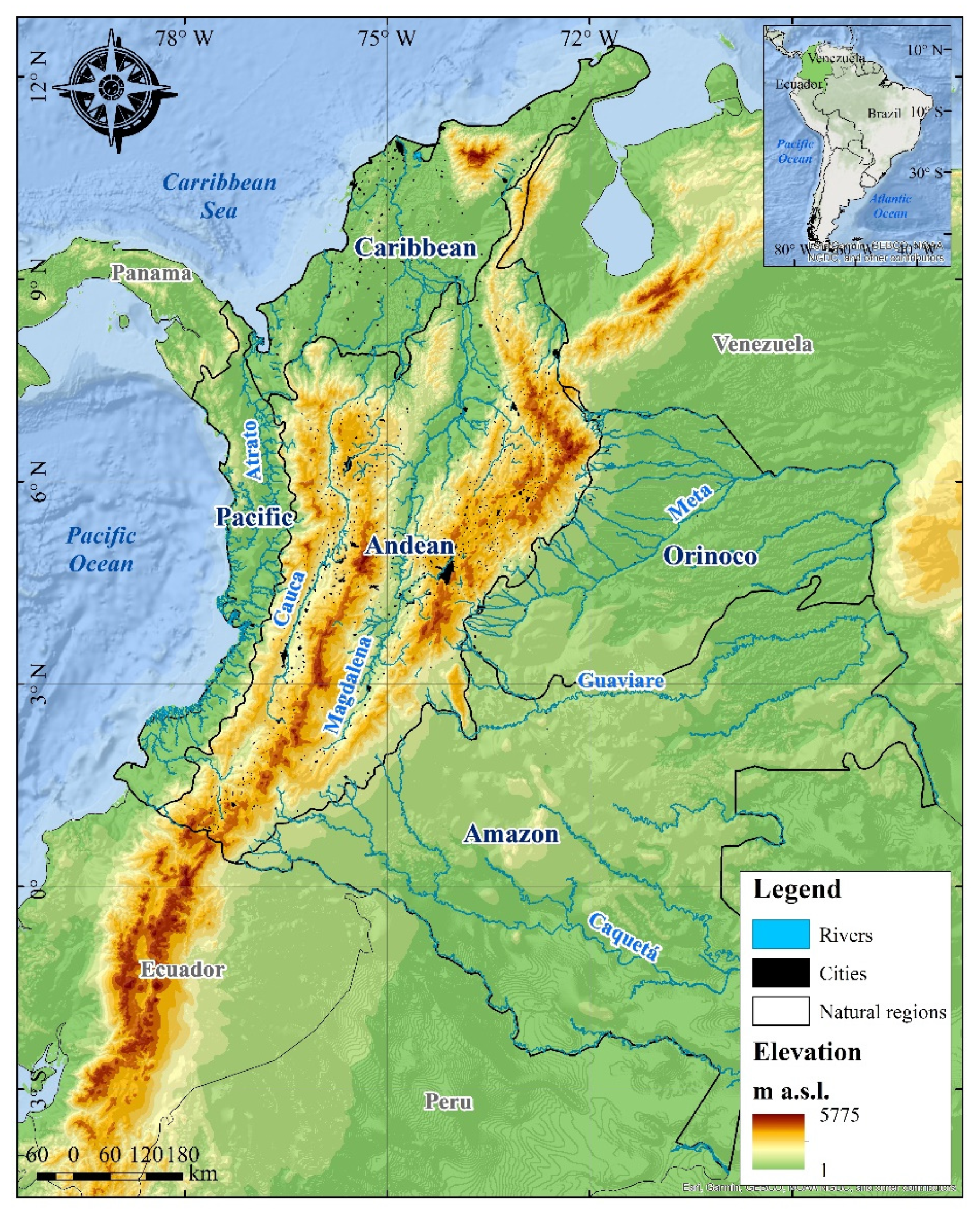
2.1. Study Area
2.2. The Climate Hazards Group Infrared Precipitation with Stations (CHIRPS)
2.3. Precipitation Extremes Indices
2.4. Trend Empirical Orthogonal Function Analysis-TEOF
2.5. Mann–Kendal (MK) Test
3. Results
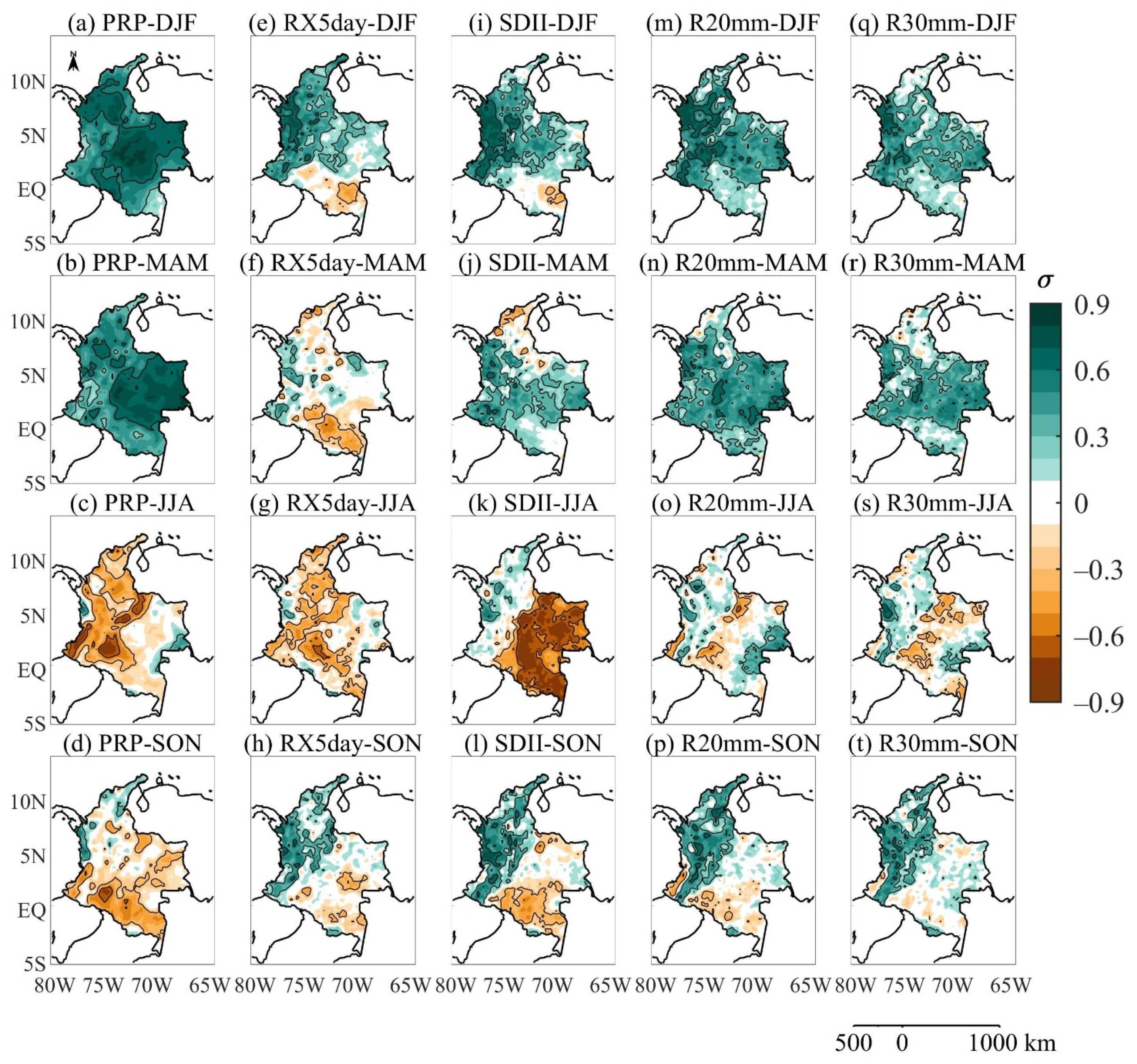
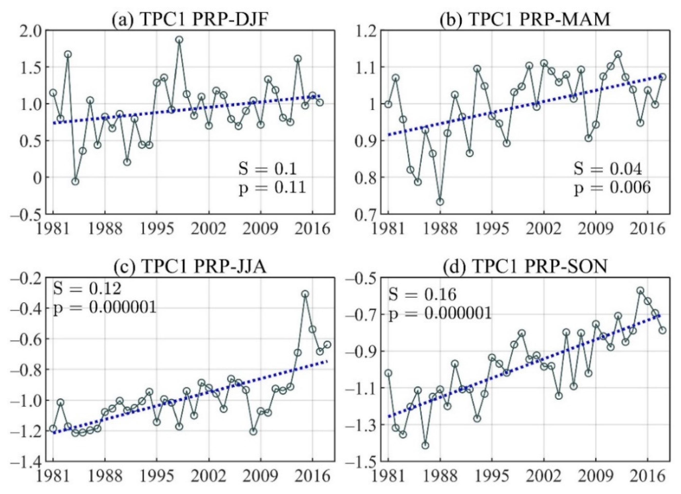
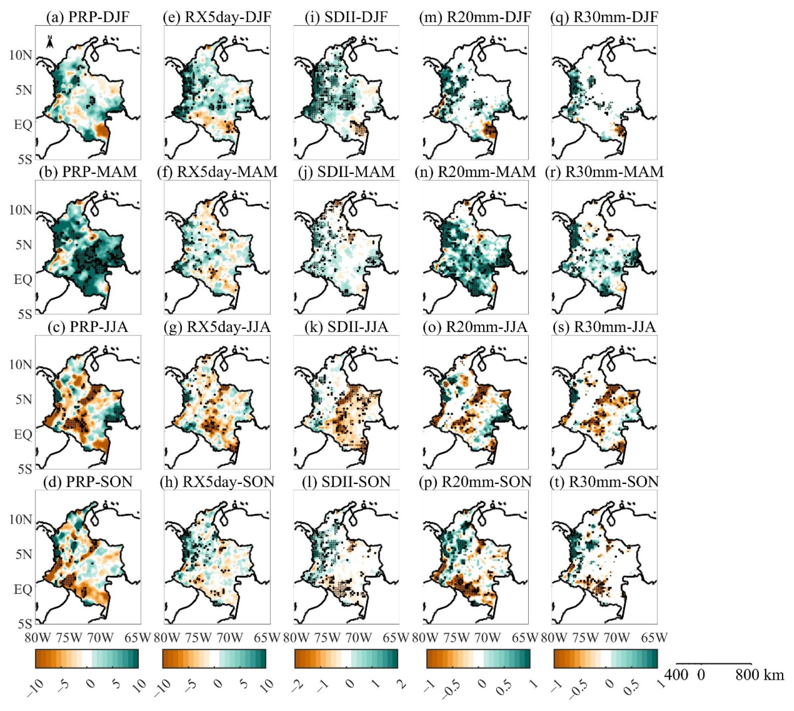
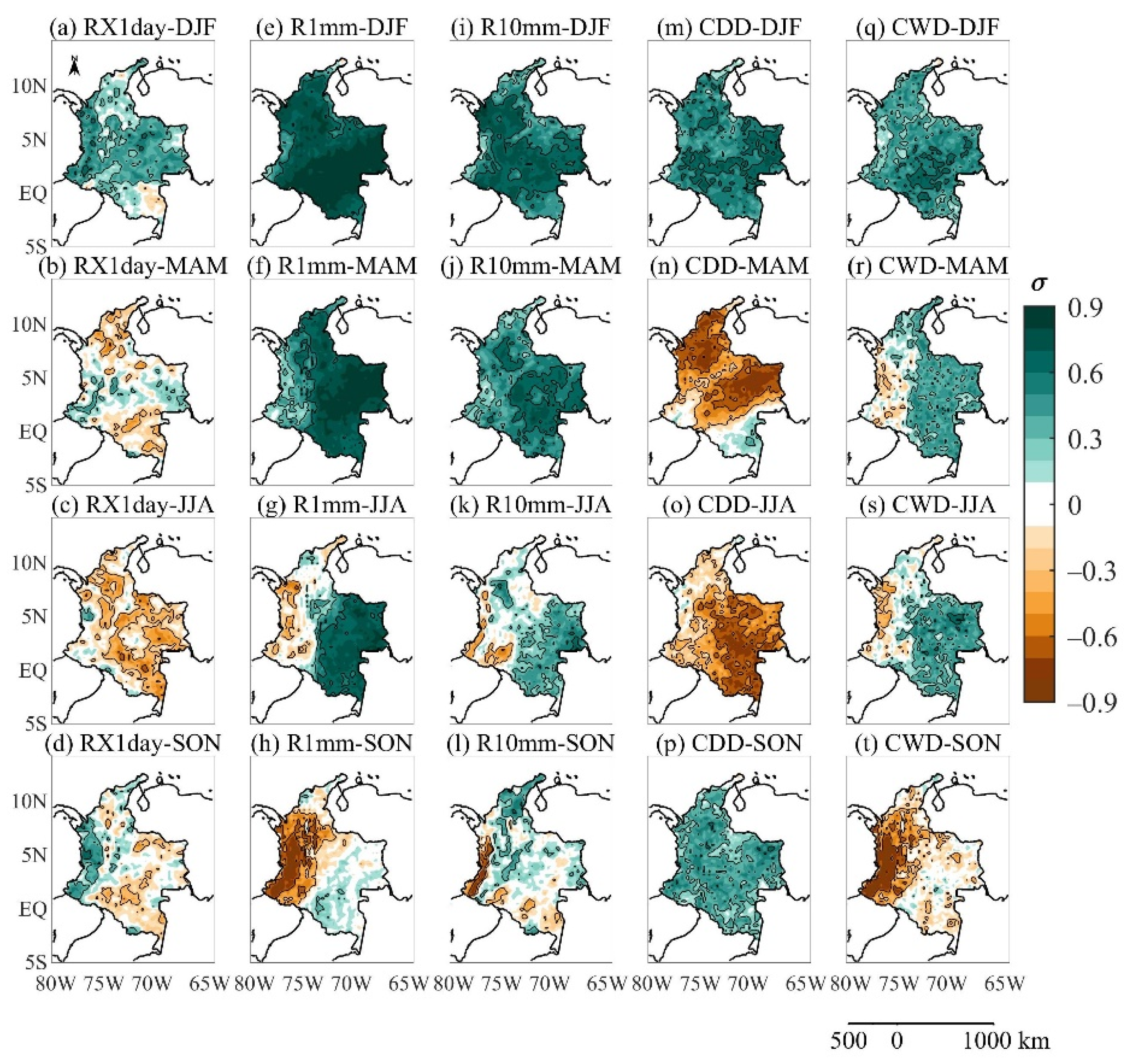
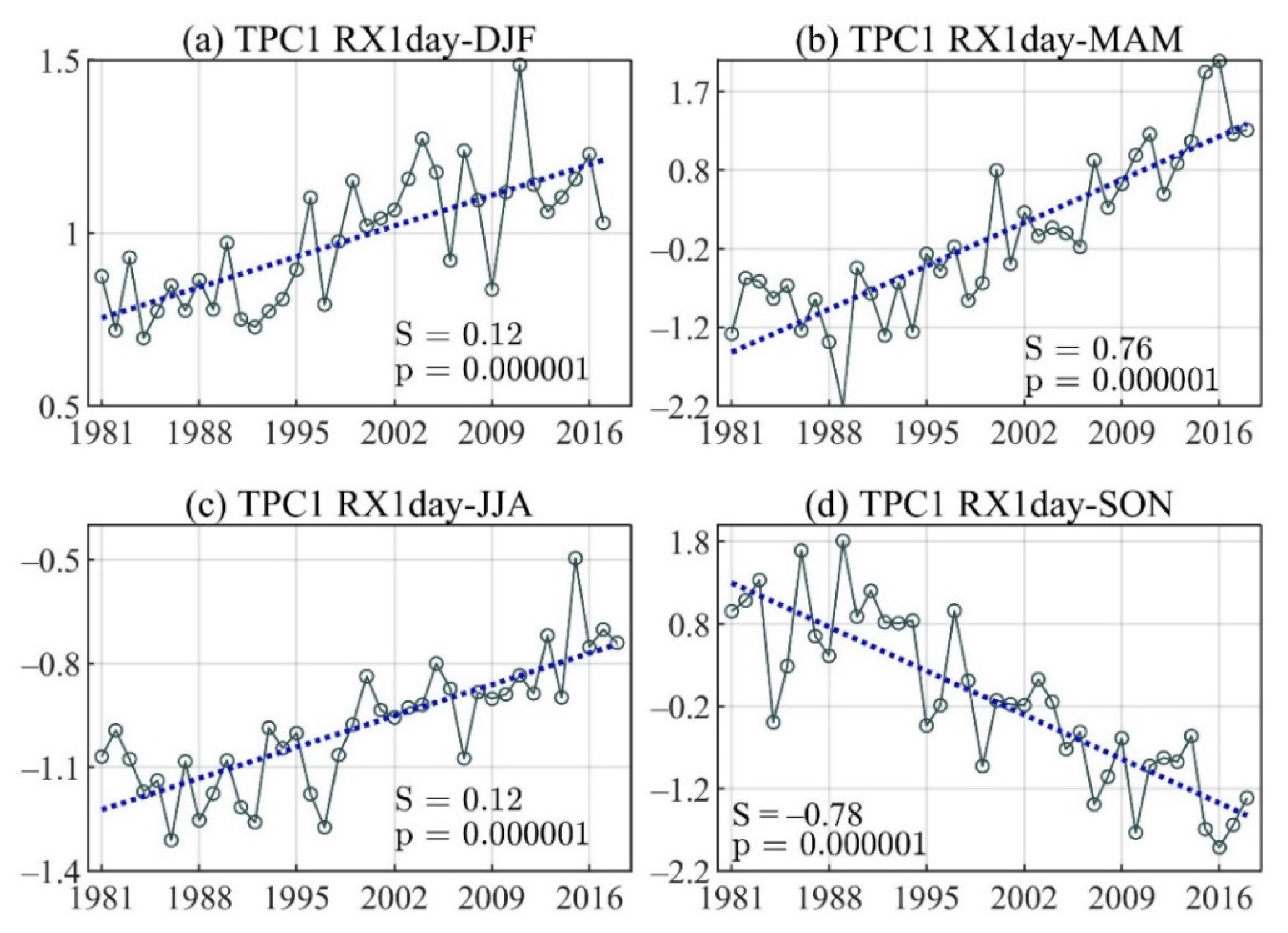
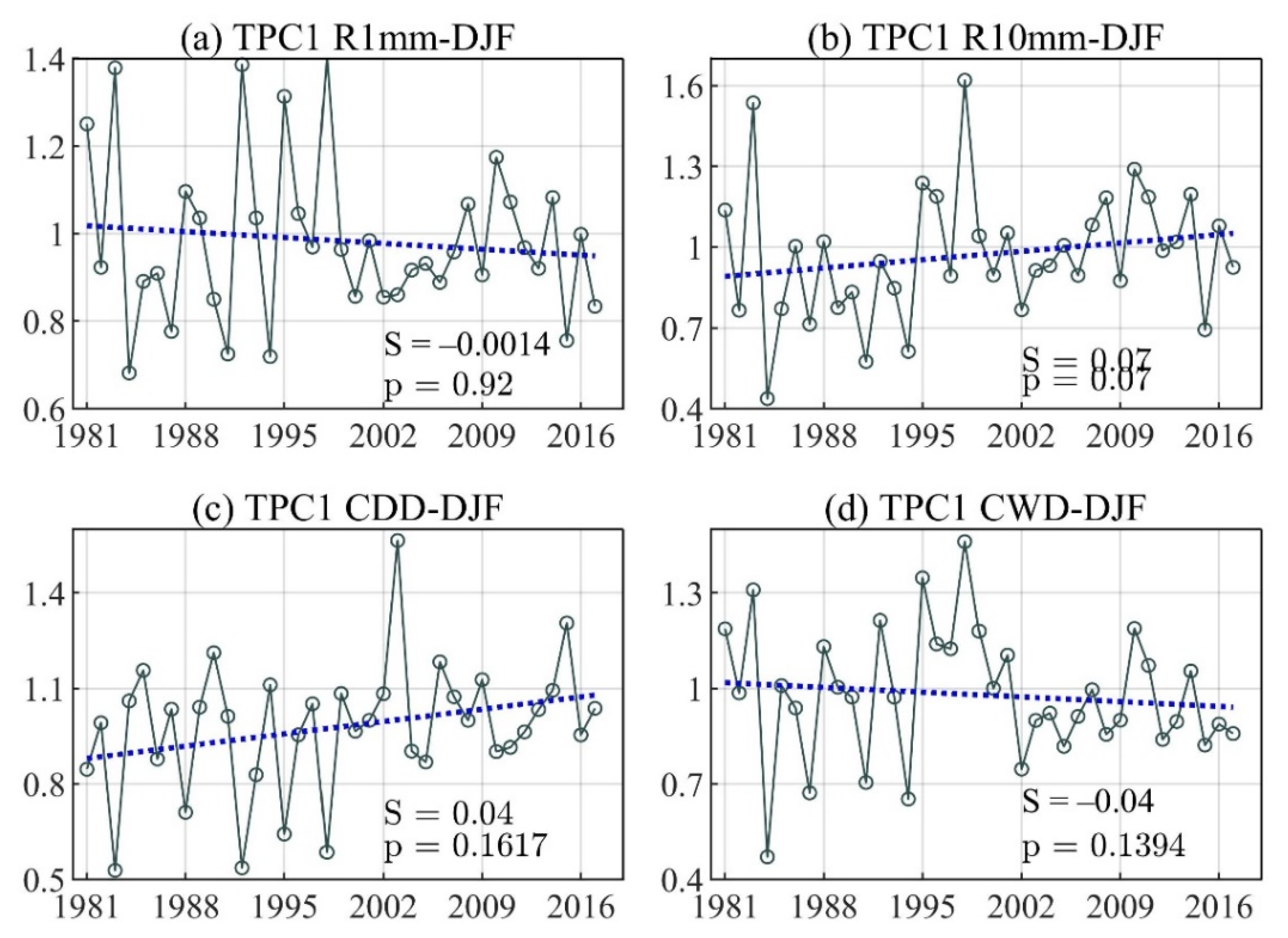
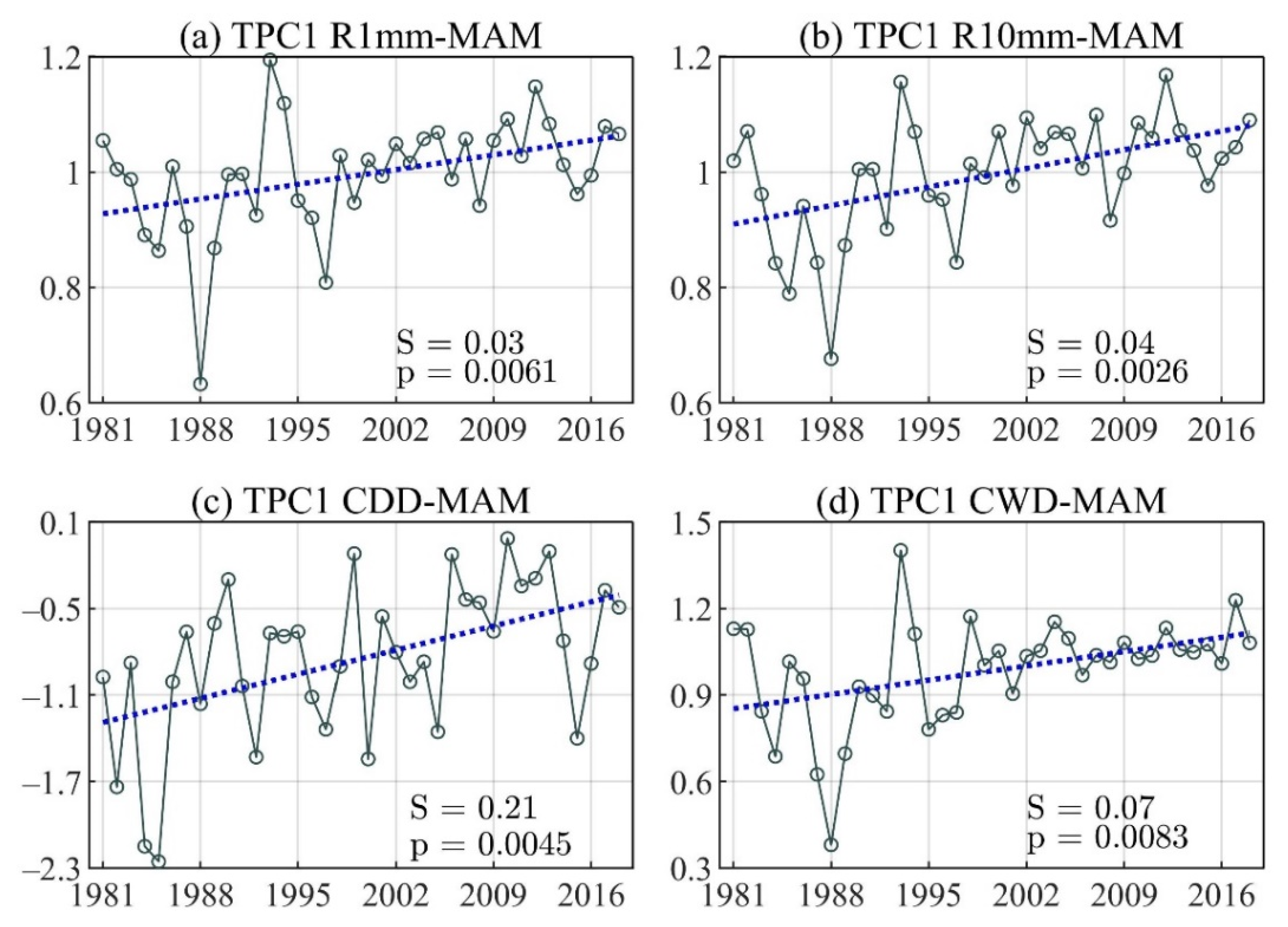
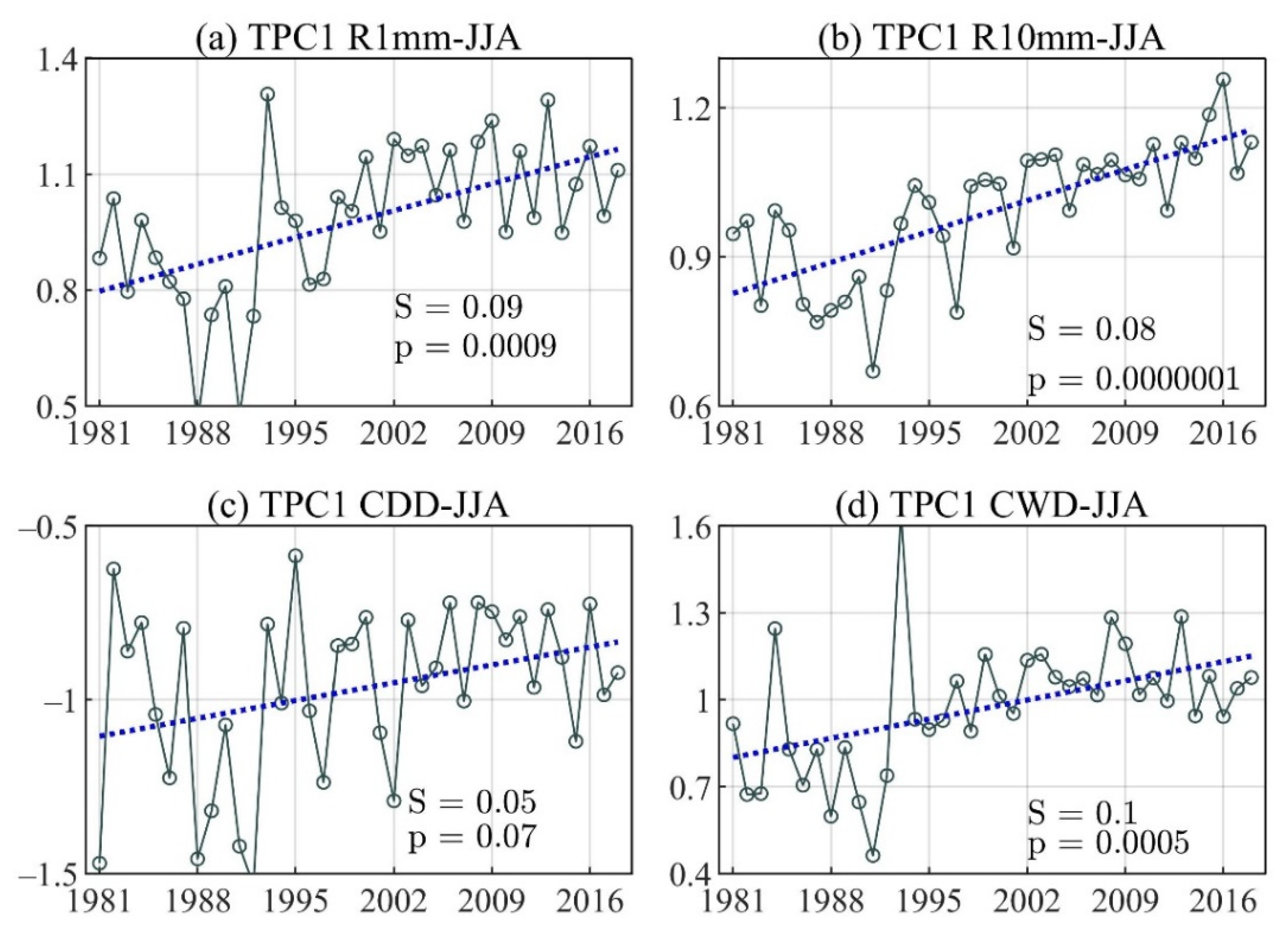
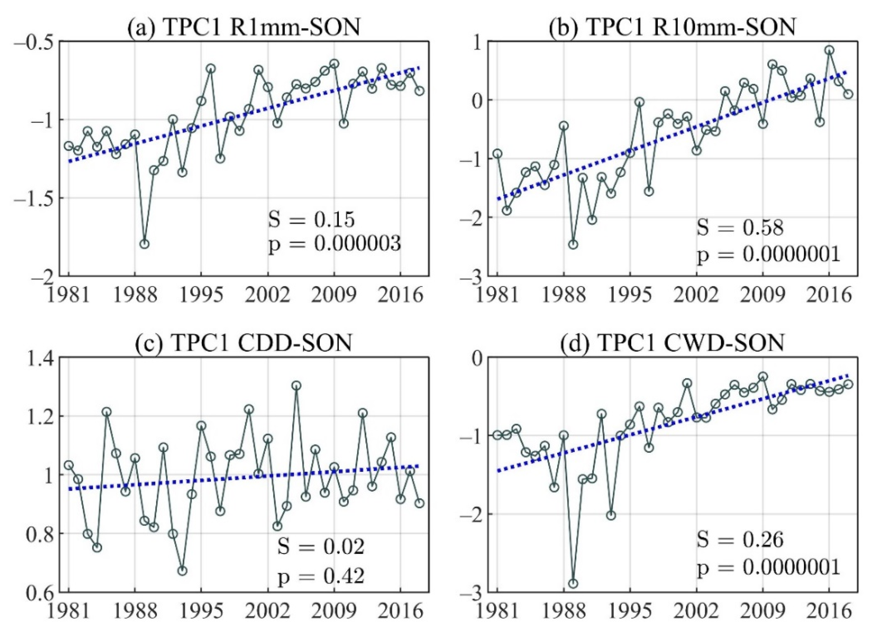
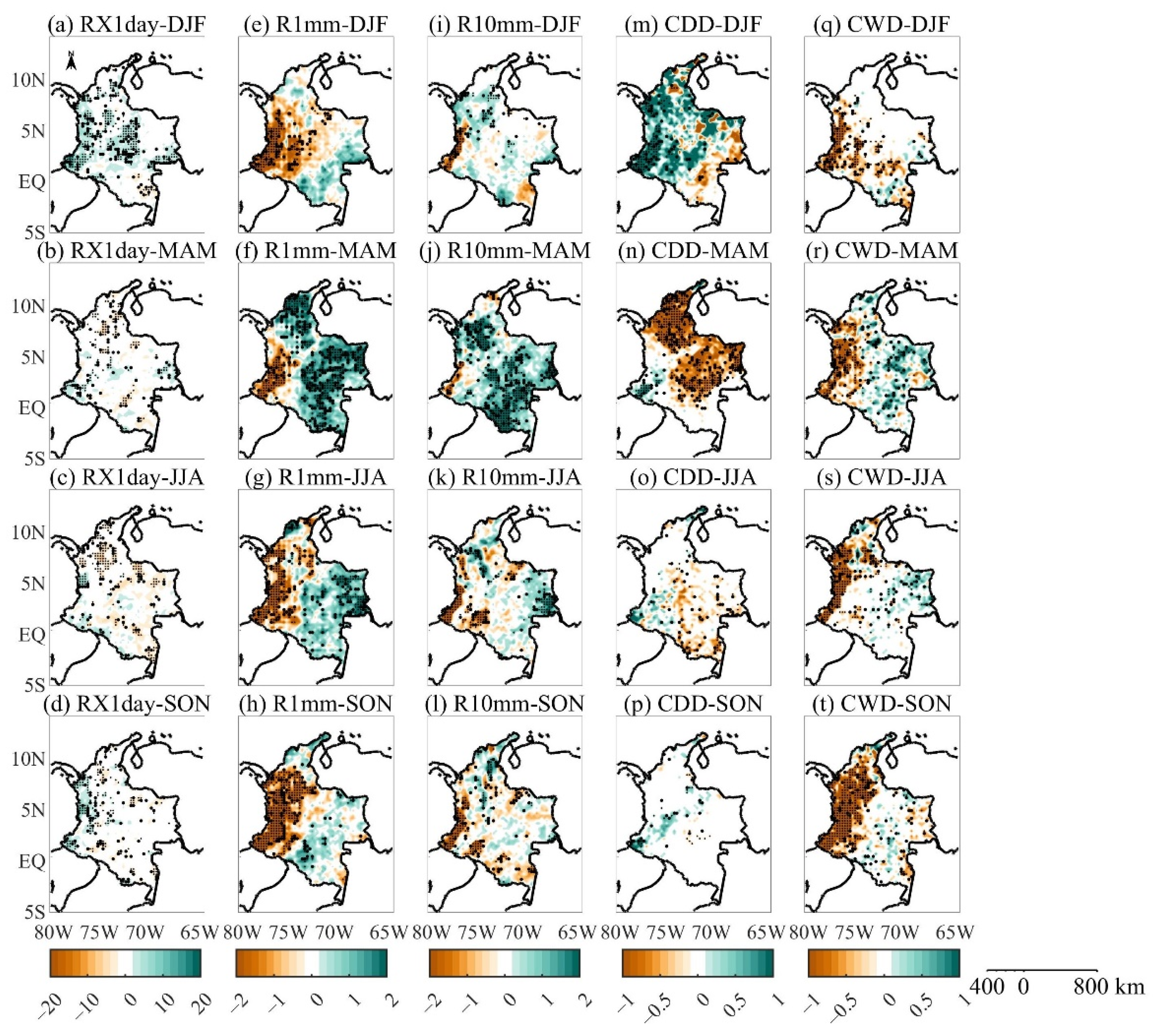
Trend Patterns
4. Discussion and Conclusions
Author Contributions
Funding
Institutional Review Board Statement
Informed Consent Statement
Data Availability Statement
Acknowledgments
Conflicts of Interest
Appendix A


References
- Seneviratne, S.I.; Zhang, X.; Adnan, M.; Badi, W.; Dereczynski, C.; Di Luca, A.; Ghosh, S.; Iskandar, I.; Kossin, J.; Lewis, S.; et al. Chapter 11: Weather and climate extreme events in a changing climate. In Climate Change 2021: The Physical Science Basis. Contribution of Working Group I to the Sixth Assessment Report of the Intergovernmental Panel on Climate Change; Masson-Delmotte, V.P., Zhai, A., Pirani, S.L., Connors, C., Péan, S., Berger, N., Caud, Y., Chen, L., Goldfarb, M.I., Gomis, M., et al., Eds.; Cambridge University Press: Cambridge, UK, 2021; p. 345, in press. [Google Scholar]
- Meehl, G.A.; Zwiers, F.; Evans, J.; Knutson, T.; Mearns, L.; Whetton, P. Trends in extreme weather and climate events: Issues related to modeling extremes in projections of future climate change. Bull. Am. Meteorol. Soc. 2000, 81, 427–436. [Google Scholar] [CrossRef] [Green Version]
- Schneider, S.H. Abrupt Non-Linear Climate Change, Irreversibility and Surprise: OECD Workshop on the Benefits of Climate Policy: Improving Information for Policy Makers; OECD: Paris, France, 2003. [Google Scholar]
- Retana, J. Eventos hidrometeorológicos extremos lluviosos en Costa Rica desde la perspectiva de la adaptación al cambio en el clima. Rev. Ciencias Ambient. 2012, 44, 5. [Google Scholar] [CrossRef] [Green Version]
- Marelle, L.; Myhre, G.; Hodnebrog, Ø.; Sillmann, J.; Samset, B.H. The Changing Seasonality of Extreme Daily Precipitation. Geophys. Res. Lett. 2018, 45, 352. [Google Scholar] [CrossRef] [Green Version]
- World Economic Forum. The Global Risks Report 2021, 16th ed.; World Economic Forum: Geneva, Switzerland, 2021; ISBN 9782940631247. [Google Scholar]
- AghaKouchak, A.; Chiang, F.; Huning, L.S.; Love, C.A.; Mallakpour, I.; Mazdiyasni, O.; Moftakhari, H.; Papalexiou, S.M.; Ragno, E.; Sadegh, M. Climate Extremes and Compound Hazards in a Warming World. Annu. Rev. Earth Planet. Sci. 2020, 48, 519–548. [Google Scholar] [CrossRef] [Green Version]
- Tabari, H. Climate change impact on flood and extreme precipitation increases with water availability. Sci. Rep. 2020, 10, 1–10. [Google Scholar] [CrossRef] [PubMed]
- Balmaceda-Huarte, R.; Olmo, M.E.; Bettolli, M.L.; Poggi, M.M. Evaluation of multiple reanalyses in reproducing the spatio-temporal variability of temperature and precipitation indices over southern South America. Int. J. Climatol. 2021, joc.7142. [Google Scholar] [CrossRef]
- Vicente-Serrano, S.M.; García-Herrera, R.; Peña-Angulo, D.; Tomas-Burguera, M.; Domínguez-Castro, F.; Noguera, I.; Calvo, N.; Murphy, C.; Nieto, R.; Gimeno, L.; et al. Do CMIP models capture long-term observed annual precipitation trends? Clim. Dyn. 2021, 1–18. [Google Scholar] [CrossRef]
- Donat, M.; Alexander, L.V.; Herold, N.; Dittus, A.J. Temperature and precipitation extremes in century-long gridded observations, reanalyses, and atmospheric model simulations. J. Geophys. Res. Atmos. 2016, 121, 11–174. [Google Scholar] [CrossRef] [Green Version]
- Wahlstrom, M.; Guha-Sapir, D. The Human Cost of Weather Related Disasters—1995–2015. 2016. Available online: https://www.unisdr.org/files/46796_cop21weatherdisastersreport2015.pdf (accessed on 13 January 2022).
- Chadwick, R.; Good, P.; Martin, G.; Rowell, D.P. Large rainfall changes consistently projected over substantial areas of tropical land. Nat. Clim. Chang. 2016, 6, 177–181. [Google Scholar] [CrossRef]
- Soares, D.; Lee, H.; Loikith, P.; Barkhordarian, A.; Mechoso, C. Can significant trends be detected in surface air temperature and precipitation over South America in recent decades? Int. J. Climatol. 2017, 37, 1483–1493. [Google Scholar] [CrossRef] [Green Version]
- Sun, Q.; Zhang, X.; Zwiers, F.; Westra, S.; Alexander, L.V. A global, continental, and regional analysis of changes in extreme precipitation. J. Clim. 2021, 34, 243–258. [Google Scholar] [CrossRef]
- Skansi, M.; Brunet, M.; Sigró, J.; Aguilar, E.; Arevalo, G.; Bentancur, O.; Castellón, G.; Correa, A.; Jácome, H.; Malheiros, R.; et al. Warming and wetting signals emerging from analysis of changes in climate extreme indices over South America. Glob. Planet. Change 2013, 100, 295–307. [Google Scholar] [CrossRef]
- Aguilar, E.; Peterson, T.; Obando, P.R.; Frutos, R.; Retana, J.A.; Solera, M.; Soley, J.; García, I.G.; Araujo, R.M.; Santos, A.R.; et al. Changes in precipitation and temperature extremes in Central America and northern South America, 1961-2003. J. Geophys. Res. Atmos. 2005, 110, 1–15. [Google Scholar] [CrossRef]
- Ávila, A.; Justino, F.; Wilson, A.; Bromwich, D.; Amorim, M. Recent precipitation trends, flash floods and landslides in southern Brazil. Environ. Res. Lett. 2016, 11, 114029. [Google Scholar] [CrossRef]
- Ávila, Á.; Guerrero, F.C.; Escobar, Y.C.; Justino, F. Recent precipitation trends and floods in the Colombian Andes. Water 2019, 11, 379. [Google Scholar] [CrossRef] [Green Version]
- Avila-Diaz, A.; Justino, F.; Lindemann, D.S.; Rodrigues, J.M.; Ferreira, G.R. Climatological aspects and changes in temperature and precipitation extremes in viçosa-Minas Gerais. An. Acad. Bras. Cienc. 2020, 92, 1–19. [Google Scholar] [CrossRef]
- Espinoza, J.C.; Ronchail, J.; Marengo, J.A.; Segura, H. Contrasting North–South changes in Amazon wet-day and dry-day frequency and related atmospheric features (1981–2017). Clim. Dyn. 2019, 52, 5413–5430. [Google Scholar] [CrossRef]
- Cerón, W.L.; Kayano, M.T.; Andreoli, R.V.; Avila-Diaz, A.; Ayes, I.; Freitas, E.D.; Martins, J.A.; Souza, R.A.F. Recent intensification of extreme precipitation events in the La Plata Basin in Southern South America (1981–2018). Atmos. Res. 2021, 249, 105299. [Google Scholar] [CrossRef]
- Campos, G.A.; Nielsen, H.N.; Díaz, G.C.; Ubiano, V.D.M.; Costa, P.C.R.; Ramírez, C.F.; Dickson, E. Análisis de la Gestión del Riesgo de Desastres en Colombia. Un Aporte para la Construcción de Políticas Públicas; Mundial, B., Ed.; Banco Mundial: Bogotá, Columbia, 2012. [Google Scholar]
- Sedano-Cruz, K.; Carvajal-Escobar, Y.; Ávila, Á. Análisis de aspectos que incrementan el riesgo de inundaciones en Colombia. Rev. Luna Azul 2013, 37, 219–238. [Google Scholar]
- Loaiza, W.; Carvajal-Escobar, Y.; Baquero, O.L. Sequías & Adaptación: Principios Para su Evaluación en Sistemas Productivos Agrícolas del Valle del Cauca, Colombia; Universidad del Valle: Cali, Columbia, 2014. [Google Scholar]
- Sanchez, O.; Aristizábal, E. Spatial and temporal paterns and socieconomic impact of landslides in Colombia. Poster Eur. Geosci. Meet 2018, 20, 3575. [Google Scholar]
- Aristizábal, E.; García, E.F.; Marín, R.J.; Gómez, F.; Guzmán-Martínez, J. Rainfall-intensity effect on landslide hazard assessment due to climate change in north-western Colombian Andes. Rev. Fac. Ing. Univ. Antioquia 2022, 51–66. [Google Scholar] [CrossRef]
- Poveda, G.; Álvarez, D.M.; Rueda, Ó.A. Hydro-climatic variability over the Andes of Colombia associated with ENSO: A review of climatic processes and their impact on one of the Earth’s most important biodiversity hotspots. Clim. Dyn. 2011, 36, 2233–2249. [Google Scholar] [CrossRef]
- Arias, P.A.; Martínez, J.A.; Vieira, S.C. Moisture sources to the 2010–2012 anomalous wet season in northern South America. Clim. Dyn. 2015, 45, 2861–2884. [Google Scholar] [CrossRef]
- Serna, L.M.; Arias, P.A.; Vieira, S.C. Las corrientes superficiales de chorro del Chocó y el Caribe durante los eventos de El Niño y El Niño Modoki. Rev. Acad. Colomb. Cienc. Exactas Físicas Nat. 2018, 42, 410. [Google Scholar] [CrossRef]
- Mesa, O.; Urrea, V.; Ochoa, A. Trends of hydroclimatic intensity in Colombia. Climate 2021, 9, 120. [Google Scholar] [CrossRef]
- Carmona, A.M.; Poveda, G. Detection of long-term trends in monthly hydro-climatic series of Colombia through Empirical Mode Decomposition. Clim. Chang. 2014, 123, 301–313. [Google Scholar] [CrossRef]
- Cantor, D.C. Evaluación y Análisis Espacio Temporal de Tendencias de Largo Plazo en la Hidroclimatología Colombiana. Master’s Thesis, Universidad Nacional de Colombia, Medellín, Colombia, 2011. [Google Scholar]
- Pabón-Caicedo, J.D. Cambio Climático en Colombia: Tendencias en la segunda mitad del siglo XX Y escenarios posibles para el siglo XXI. Rev. Acad. Colomb. Cienc. Exactas Físicas Nat. 2012, 36, 261–278. [Google Scholar]
- Mayorga, R.; Hurtado, G.M.; Benavides, H. Evidencias de Cambio Climático en Colombia Con Base en Información Estadística. 2011. Available online: http://www.ideam.gov.co/documents/21021/21138/Evidencias+de+Cambio+Clim%C3%A1tico+en+Colombia+con+base+en+informaci%C3%B3n+estad%C3%ADstica.pdf/1170efb4-65f7-4a12-8903-b3614351423f (accessed on 13 January 2022).
- IDEAM PNUD MADS DNP CANCILLERÍA Tercera Comunicación Nacional de Colombia, Resumen Ejecutivo a la Convención Marco de las Naciones Unidas Sobre Cambio Climático; Bogotá (Colombia). 2017. Available online: http://documentacion.ideam.gov.co/openbiblio/bvirtual/023732/RESUMEN_EJECUTIVO_TCNCC_COLOMBIA.pdf (accessed on 13 January 2022).
- Morales-Acuña, E.; Linero-Cueto, J.R.; Canales, F.A. Assessment of precipitation variability and trends based on satellite estimations for a heterogeneous Colombian region. Hydrology 2021, 8, 128. [Google Scholar] [CrossRef]
- Coronado-Hernández, Ó.E.; Merlano-Sabalza, E.; Díaz-Vergara, Z.; Coronado-Hernández, J.R. Selection of hydrological probability distributions for extreme rainfall events in the regions of Colombia. Water 2020, 12, 1397. [Google Scholar] [CrossRef]
- Hannachi, A. Pattern hunting in climate: A new method for finding trends in gridded climate data. Int. J. Climatol. 2007, 27, 1–15. [Google Scholar] [CrossRef]
- IGAC Instituto Geográfico Agustín Codazzi Regiones Naturales. Available online: http://www2.igac.gov.co/ninos/UserFiles/Image/Mapas/regiones%20naturales.pdf (accessed on 13 January 2022).
- Urrea, V.; Ochoa, A.; Mesa, O. Seasonality of Rainfall in Colombia. Water Resour. Res. 2019, 55, 4149–4162. [Google Scholar] [CrossRef]
- Cerón, W.L.; Andreoli, R.V.; Kayano, M.T.; Avila-Diaz, A. Role of the eastern Pacific-Caribbean Sea SST gradient in the Choco low-level jet variations from 1900–2015. Clim. Res. 2021, 83, 61–74. [Google Scholar] [CrossRef]
- Yepes, J.; Poveda, G.; Mejía, J.F.; Moreno, L.; Rueda, C. Choco-jex: A research experiment focused on the Chocó low-level jet over the far eastern Pacific and western Colombia. Bull. Am. Meteorol. Soc. 2019, 100, 779–796. [Google Scholar] [CrossRef]
- Estupiñan, A.R.C. Estudio de la Variabilidad Espacio Temporal de la Precipitación en Colombia. Doctoral Dissertation, Universidad Nacional de Colombia. 2016. Available online: http://bdigital.unal.edu.co/54014/1/1110490004.2016.pdf (accessed on 5 October 2019).
- Mejía, J.; Mesa, O.J.; Poveda, G.; Vélez, J.I.; Hoyos, C.; Ricardo, M.; Barco, J.; Cuartas, A.; Montoya, M.; Botero, B. Distribución espacial y ciclos anual y semianual de la precipitación en Colombia. Dyna 1999, 127, 7–26. [Google Scholar]
- Climate Hazards Group Infrared Precipitation with Stations (CHIRPS) CHIRPS Data. Available online: https://www.chc.ucsb.edu/data/chirps/ (accessed on 6 June 2020).
- Funk, C.; Verdin, A.; Michaelsen, J.; Peterson, P.; Pedreros, D. A global satellite assisted precipitation climatology. Earth Syst. Dyn. Discuss. 2015, 8, 401–425. [Google Scholar] [CrossRef] [Green Version]
- Funk, C.; Peterson, P.; Landsfeld, M.; Pedreros, D.; Verdin, J.; Shukla, S.; Husak, G.; Rowland, J.; Harrison, L.; Hoell, A.; et al. The climate hazards infrared precipitation with stations—A new environmental record for monitoring extremes. Sci. Data 2015, 2, 150066. [Google Scholar] [CrossRef] [PubMed] [Green Version]
- Urrea, V.; Ochoa, A.; Mesa, O. Validación de la base de datos de precipitación CHIRPS para Colombia a escala diaria, mensual y anual en el período 1981–2014 Conference. In Proceedings of the XXVII Congreso Latinoamericano de Hidráulica, San Isidro, Peru, 26–30 September 2016; pp. 1–12. [Google Scholar]
- Cerón, W.L.; Kayano, M.T.; Andreoli, R.V.; Canchala, T.; Carvajal-Escobar, Y.; Alfonso-Morales, W. Rainfall variability in Southwestern Colombia: Changes in ENSO—Related features. Pure Appl. Geophys. 2021, 178, 1–17. [Google Scholar] [CrossRef]
- Fernandes, K.; Muñoz, A.G.; Ramirez-Villegas, J.; Agudelo, D.; Llanos-Herrera, L.; Esquivel, A.; Rodriguez-Espinoza, J.; Prager, S.D. Improving seasonal precipitation forecasts for agriculture in the orinoquía Region of Colombia. Weather Forecast. 2020, 35, 437–449. [Google Scholar] [CrossRef]
- Zhang, X.; Yang, F.; Canada, E. RClimDex (1.0) User Manual; Climate Research Branch, Environment Canada: Downsview, ON, Canada, 2004; pp. 1–23. [Google Scholar]
- Poveda, G.; Vélez, J.I.; Mesa, O.; Hoyos, C.; Mejía, J.; Barco, O.J.; Correa, P.L. Influencia de fenómenos macroclimáticos sobre el ciclo anual de la hidrología Colombiana: Cuantificación lineal, no lineal y percentiles probabilísticos. Meteorol. Colomb. 2002, 121–130. [Google Scholar]
- Poveda, G.; Waylen, P.R.; Pulwarty, R.S. Annual and inter-annual variability of the present climate in northern South America and southern Mesoamerica. Palaeogeogr. Palaeoclimatol. Palaeoecol. 2006, 234, 3–27. [Google Scholar] [CrossRef]
- Poveda, G. La hidroclimatología de Colombia: Una síntesis desde la escala inter-decadal hasta la escala diurna. Rev. Académica Colomb. Ciencias Tierra 2004, 28, 201–222. Available online: https://www.researchgate.net/publication/284691636_La_hidroclimatologia_de_Colombia_Una_sintesis_desde_la_escala_inter-decadal_hasta_la_escala_diurna (accessed on 13 January 2022).
- Guzmán, D.; Ruíz, J.F.; Cadena, M. Regionalización de Colombia según la Estacionalidad de la Precipitación Media Mensual, a Través Análisis de Componentes Principales (ACP); IDEAM: Bogotá, Colombia, 2014. [Google Scholar]
- Cerón, W.L.; Andreoli, R.V.; Kayano, M.T.; de Ferreria, S.R.; Canchala, N.T.; Carvajal-Escobar, Y. Comparison of spatial interpolation methods for annual and seasonal rainfall in two hotspots of biodiversity in South America. An. Acad. Bras. Ciencias 2021, 93, 1–22. [Google Scholar] [CrossRef] [PubMed]
- Valverde, M.C.; Marengo, J.A. Extreme Rainfall Indices in the Hydrographic Basins of Brazil. Open J. Mod. Hydrol. 2014, 04, 10–26. [Google Scholar] [CrossRef] [Green Version]
- Cerón, W.L.; Kayano, M.T.; Andreoli, R.V.; Avila, A.; Canchala, T.; Francés, F.; Ayes Rivera, I.; Alfonso-Morales, W.; Ferreira de Souza, R.A.; Carvajal-Escobar, Y. Streamflow Intensification Driven by the Atlantic Multidecadal Oscillation (AMO) in the Atrato River Basin, Northwestern Colombia. Water 2020, 12, 216. [Google Scholar] [CrossRef] [Green Version]
- Espírito Santo, F.; Ramos, A.M.; de Lima, M.I.P.; Trigo, R.M. Seasonal changes in daily precipitation extremes in mainland Portugal from 1941 to 2007. Reg. Environ. Chang. 2014, 14, 1765–1788. [Google Scholar] [CrossRef]
- Wang, R.; Li, C. Spatiotemporal analysis of precipitation trends during 1961–2010 in Hubei province, central China. Theor. Appl. Climatol. 2016, 124, 385–399. [Google Scholar] [CrossRef]
- Donat, M.G.; Angélil, O.; Ukkola, A.M. Intensification of precipitation extremes in the world’s humid and water-limited regions. Environ. Res. Lett. 2019, 14, 065003. [Google Scholar] [CrossRef]
- Naciones Unidas CEPAL. Efectos del Cambio Climático en la Costa de América Latina y el Caribe Efectos del Cambio Climático en la costa de América Latina y el Caribe: Dinámicas, Tendencias y Variabilidad Climática; CEPAL: Santander, España, 2011; Volume 447. [Google Scholar]
- Barbosa, S.M.; Andersen, O.B. Trend patterns in global sea surface temperature. Int. J. Climatol. 2009, 29, 2049–2055. [Google Scholar] [CrossRef]
- Latif, M.; Syed, F.S.; Hannachi, A. Rainfall trends in the South Asian summer monsoon and its related large-scale dynamics with focus over Pakistan. Clim. Dyn. 2017, 48, 3565–3581. [Google Scholar] [CrossRef]
- Mann, H.B. Nonparametric Tests Against Trend. Econometrica 1945, 13, 245–259. [Google Scholar] [CrossRef]
- Kendall, M.G. Rank Correlation Methods, 4th ed.; Griffin: London, UK, 1975; ISBN 0852641990. [Google Scholar]
- Theil, H. A rank-invariant method of linear and polynomial regression analysis, 3; confidence regions for the parameters of polynomial regression equations. Indag. Math. 1950, 1, 467–482. [Google Scholar]
- Theil, H. A Rank-Invariant Method of Linear and Polynomial Regression Analysis. In Advanced Studies in Theoretical and Applied Econometrics; Raj, B., Koerts, J., Eds.; Henri Theil’s Contributions to Economics and Econometrics; Springer: Dordrecht, The Netherlands, 1992; Volume 23. [Google Scholar]
- Sen, P.K. Estimates of the Regression Coefficient Based on Kendall’s Tau. J. Am. Stat. Assoc. 1968, 63, 1379–1389. [Google Scholar] [CrossRef]
- Jonah, K.; Wen, W.; Shahid, S.; Ali, M.A.; Bilal, M.; Habtemicheal, B.A.; Iyakaremye, V.; Qiu, Z.; Almazroui, M.; Wang, Y.; et al. Spatiotemporal variability of rainfall trends and influencing factors in Rwanda. J. Atmos. Sol.-Terr. Phys. 2021, 219, 105631. [Google Scholar] [CrossRef]
- Endo, N.; Ailikun, B.; Yasunari, T. Trends in precipitation amounts and the number of rainy days and heavy rainfall events during summer in China from 1961 to 2000. J. Meteorol. Soc. Japan 2005, 83, 621–631. [Google Scholar] [CrossRef] [Green Version]
- Rajeevan, M.; Bhate, J.; Jaswal, A.K. Analysis of variability and trends of extreme rainfall events over India using 104 years of gridded daily rainfall data. Geophys. Res. Lett. 2008, 35, 1–6. [Google Scholar]
- Doyle, M.E.; Saurral, I.; Barros, V.R. Trends in the distributions of aggregated monthly precipitation over the La Plata Basin. Int. J. Climatol. 2012, 32, 2149–2162. [Google Scholar] [CrossRef]
- Estupiñan, A.; Carvajal-Serna, L.F. Evaluación de las tendencias de largo plazo en la cuenca del río Aburra (Medellin-Colombia) durante el período 1981–2017. In Proceedings of the XXVIII Congr. Latinoamericano Hidráulica, Buenos Aires, Argentina, 18–21 September 2018. [Google Scholar]
- García Múnera, V.; Arias Gómez, P.; Vieria Agudelo, S. Análisis de tendencias en series de precipitación y tempertura de la Cuenca del Río Grande—Antioquía. In Proceedings of the XXII Seminario Nacional de Hidraúlica e Hidrología. Sociedad Colombiana de Ingenieros, Bogotá, Colombia, 24–26 August 2016; p. 13. [Google Scholar]
- Cardona, F.; Ávila, Á.J.; Carvajal-Escobar, Y.; Jiménez, H. Tendencias en las series de precipitación en dos cuencas torrenciales andinas del Valle del Cauca (Colombia). Tecno Lógicas 2014, 17, 85–95. [Google Scholar] [CrossRef]
- Puertas, O.O.; Carvajal-Escobar, Y.; Quintero, A.M. Estudio de tendencias de la precipitación mensual en la cuenca alta-media del río Cauca, Colombia. DYNA 2011, 78, 112–120. [Google Scholar]
- Rojas, E.; Arce, B.; Peña, A.; Boshell, F.; Ayarza, M. Cuantificación e interpolación de tendencias locales de temperatura y precipitación en zonas alto andinas de Cundinamarca y Boyacá (Colombia). Corpoica Cienc. Tecnol. Agropecu. 2010, 11, 173. [Google Scholar] [CrossRef] [Green Version]
- Arrieta-Castro, M.; Donado-Rodríguez, A.; Acuña, G.J.; Canales, F.A.; Teegavarapu, R.S.V.; Kaźmierczak, B. Analysis of streamflow variability and trends in the meta river, Colombia. Water 2020, 12, 1451. [Google Scholar] [CrossRef]
- Li, G.; Ren, B. Evidence for strengthening of the tropical Pacific Ocean surface wind speed during 1979-2001. Theor. Appl. Climatol. 2012, 107, 59–72. [Google Scholar] [CrossRef]


| Indices | Description | Definition | Unit |
|---|---|---|---|
| (a) Intensity | |||
| RX1day | Max 1-day precipitation amount | Maximum precipitation in 1 day during L | mm |
| RX5day | Max 5-day precipitation amount | Maximum precipitation in 5 consecutive days during L | mm |
| SDII | Simple daily intensity index | Ratio of PRCPTOT 1 and the number of wet days (RR 2 ≥ 1 mm) during L | mm day−1 |
| (b) Frequency | |||
| R1mm | Number of wet days | Number of days with RR ≥ 1 mm during L | Days |
| R10mm | Number of days with precipitations above R10mm | Number of days with RR ≥ 10 mm during L | Days |
| R20mm | Number of days with precipitations above R20mm | Number of days with RR ≥ 20 mm during L | Days |
| R30mm | Number of days with precipitations above 30 mm (R30mm) | Number of days with RR ≥ 30 mm during L | Days |
| (c) Duration | |||
| CDD | Consecutive dry days | Maximum number of consecutive days when precipitation RR < 1 mm | Days |
| CWD | Consecutive wet days | Maximum number of consecutive days when precipitation RR < 1 mm | Days |
Publisher’s Note: MDPI stays neutral with regard to jurisdictional claims in published maps and institutional affiliations. |
© 2022 by the authors. Licensee MDPI, Basel, Switzerland. This article is an open access article distributed under the terms and conditions of the Creative Commons Attribution (CC BY) license (https://creativecommons.org/licenses/by/4.0/).
Share and Cite
Cerón, W.L.; Andreoli, R.V.; Kayano, M.T.; Canchala, T.; Ocampo-Marulanda, C.; Avila-Diaz, A.; Antunes, J. Trend Pattern of Heavy and Intense Rainfall Events in Colombia from 1981–2018: A Trend-EOF Approach. Atmosphere 2022, 13, 156. https://doi.org/10.3390/atmos13020156
Cerón WL, Andreoli RV, Kayano MT, Canchala T, Ocampo-Marulanda C, Avila-Diaz A, Antunes J. Trend Pattern of Heavy and Intense Rainfall Events in Colombia from 1981–2018: A Trend-EOF Approach. Atmosphere. 2022; 13(2):156. https://doi.org/10.3390/atmos13020156
Chicago/Turabian StyleCerón, Wilmar L., Rita V. Andreoli, Mary T. Kayano, Teresita Canchala, Camilo Ocampo-Marulanda, Alvaro Avila-Diaz, and Jean Antunes. 2022. "Trend Pattern of Heavy and Intense Rainfall Events in Colombia from 1981–2018: A Trend-EOF Approach" Atmosphere 13, no. 2: 156. https://doi.org/10.3390/atmos13020156