An Application of Artificial Neural Network to Evaluate the Influence of Weather Conditions on the Variation of PM_2.5-Bound Carbonaceous Compositions and Water-Soluble Ionic Species

Abstract

Previous studies have determined biomass burning as a major source of air pollutants in the ambient air in Thailand. To analyse the impacts of meteorological parameters on the variation of carbonaceous aerosols and water-soluble ionic species (WSIS), numerous statistical models, including a source apportionment analysis with the assistance of principal component analysis (PCA), hierarchical cluster analysis (HCA), and artificial neural networks (ANNs), were employed in this study. A total of 191 sets of PM_2.5 samples were collected from the three monitoring stations in Chiang-Mai, Bangkok, and Phuket from July 2020 to June 2021. Hotspot numbers and other meteorological parameters were obtained using NOAA-20 weather satellites coupled with the Global Land Data Assimilation System. Although PCA revealed that crop residue burning and wildfires are the two main sources of PM_2.5, ANNs highlighted the importance of wet deposition as the main depletion mechanism of particulate WSIS and carbonaceous aerosols. Additionally, Mg²⁺ and Ca²⁺ were deeply connected with albedo, plausibly owing to their strong hygroscopicity as the CCNs responsible for cloud formation.

1. Introduction

Previous research has underlined air quality deterioration episodes in Southeast Asian countries as a consequence of hotspot numbers [1,2,3,4,5]. Geographic information system hotspot analysis has become a powerful approach for the comprehensive assessment of the geographic consolidation of biomass burning, particularly in the Greater Mekong Subregion, which includes Thailand, Myanmar, Cambodia, Lao People’s Democratic Republic, Vietnam, and China [6,7,8]. While hotspot numbers are among the main contributors of particulate chemical species, especially in the middle of haze episodes [9,10,11], little is known about the impact of other meteorological parameters, such as relative humidity (RH), ambient temperature (T), albedo, and wind direction (WD), on variations in carbonaceous aerosols and water-soluble ionic species (WSISs), especially in tropical atmospheric environments.

Earlier findings have also shown that wet deposition plays a major role in the removal of NH₄⁺, Cl⁻, SO₄²⁻, and NO₃⁻ in the tropical atmosphere of Southeast Asia [11]. A deliberate investigation of the scavenging coefficients measured in this study indicated that the wet deposition of particulate WSIS was dramatically affected by the precipitation intensity and was aerosol size-dependent [11]. The WD can greatly enhance the atmospheric contents of some WSIS, such as SO₄²⁻, Cl⁻, Mg²⁺, K⁺, and Ca²⁺, in clouds from a tropical montane cloud forest in Puerto Rico, particularly when air masses originate from Northwest Africa [12]. The alteration of the chemical constituents and physicochemical properties of the clouds related to these various classifications of particulate matters can influence cloud formation and processes [12]. Apart from rainfall and WD, numerous meteorological parameters can also influence the variation in WSIS and carbonaceous particles. The impacts of non-sea salt sulphate, sea salt, and the total aerosol on backscattering albedo efficiency have been thoroughly examined during the first aerosol characterisation experiment (ACE1) from November to December 1995 in the Southern Ocean region south of Australia [13]. The degree of scattering by both submicron and super-micron particles is predominantly governed by the type of WSIS in maritime aerosols [13]. Field observations of the aerosol optical properties and WSIS contents in aerosols at a resolution of 1 h from April to May 2020 in urban Shanghai showed a positive linear relationship between the mass concentrations of SO₄²⁻, NO₃⁻, Cl⁻, and NH₄⁺ and the absorption coefficient at 532 nm (α_a,532) [14]. These findings underline the importance of WSIS as one of the major factors affecting the albedo coefficient and, thus, lead to a comparatively strong control of regional climate.

Artificial Neural Networks (ANNs) (i.e., recursive neural network, feedforward neural network (FNN), and multiple linear regression analysis (MLRA)) and nonlinear autoregressive models are extremely useful algorithms for the precise forecasting of respiratory mortality and mobility associated with exposure to NO₂, SO₂, O₃, PM₁₀, and PM_2.5 [15,16,17,18]. A multilayer perceptron (MLP), which is an entirely related class of FNNs, has been applied to the long-term forecasting of ambient particles and trace gaseous species with the assistance of weather conditions and source emission predictors [19]. An increasingly large portion of source apportionment research is currently focused on the application of ANNs, because this technique can assess the environmental quality by avoiding extreme evaluation results and employing fuzzy rules to eliminate the impact of pollutant concentrations that are too high or too low [20]. Despite the rapid increase in publications related to the application of ANNs in the field of source apportionment, no study has evaluated the influence of weather conditions on the variations in particulate WSIS and carbonaceous aerosols using combined PCA and ANNs. The major objectives of this study were to (i) chemically characterise particulate WSIS and other carbonaceous fractions and (ii) employ PCA and ANNs to assess the influence of meteorological parameters on the variation of chemical constituents in PM_2.5 collected at Chiang-Mai, Bangkok, and Phuket.

• Significant increases in OC, EC, and WSIS were observed during haze episodes.
• Crop residue burning and wildfires are the two main sources of PM_2.5.
• Wet deposition is the main depletion mechanism for OC, EC, and WSIS.
• Ca²⁺ and Mg²⁺ are deeply connected with albedo.

2. Materials and Methodologies

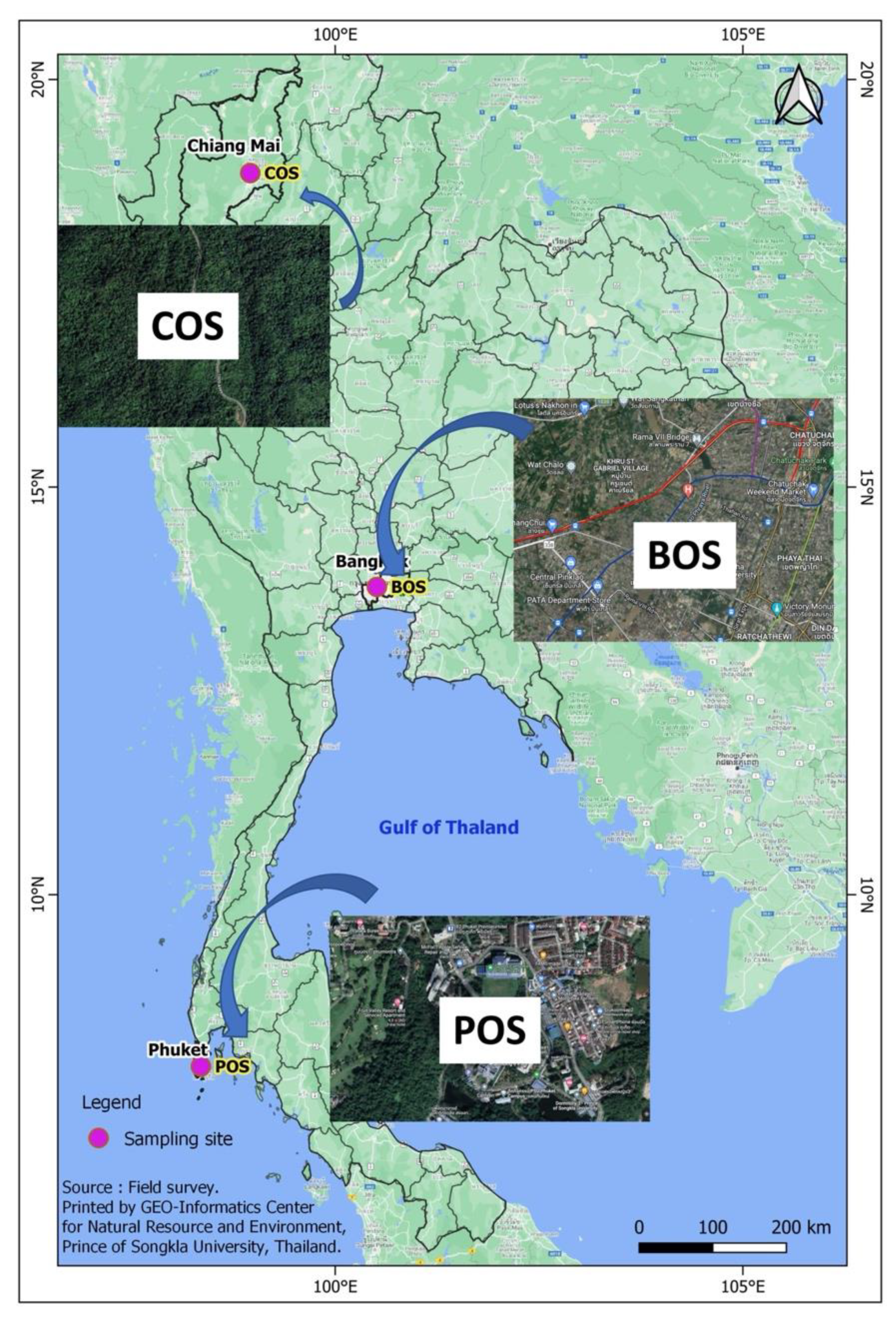
2.1. Air Monitoring Locations

To gather PM_2.5 data in a real-world situation, the suitable site must be selected based on a set of relevant criteria. The objective of any air quality observatory site selection process is to collect and evaluate the information that would subsequently lead one to draw informed conclusions regarding the selection of the most suitable site for the location of the sampling equipment. Three air quality observatory sites were carefully chosen in Thailand, from north to south: the Chiang-Mai Air Quality Observatory Site (COS), Bangkok Air Quality Observatory Site (BOS), and Phuket Air Quality Observatory Site (POS) (Figure 1). The COS is situated at the National Astronomical Research Institute of Thailand (NARIT) on top of the Doi-Inthanon Mountain, Chiang-Mai Province (18.62994° N, 98.49559° E), which is a part of the Himalayas and is 800–2565 m above sea level. Doi-Inthanon has been recognised as ‘The Roof of Thailand’, covering an area of 482 km². The COS is located on the roofs of three-storeyed NARIT office buildings (~10 m aboveground). Over the past few years, agricultural waste burning has sent the air quality in the nine northern administrative provinces to a level acknowledged harmful to cause adverse human health impact, as Chiang-Mai recorded the air quality that was among the world’s worst. In contrast, BOS is located in front of the Faculty of Science and Technology, Suan Sunandha Rajabhat University (SSRU) (13.77491° N, 100.50884° E), which is ~1.5 m above the ground level. SSRU is situated in the metropolis of Bangkok (population > 10.7 million) and close to several tourist hotspots, such as the Temple of the Emerald Buddha (Wat Phra Kaew) and Grand Palace. Bangkok, the capital of Thailand, is an extremely heavily crowded city with a population of more than 10.5 million people evaluated to be residing there in 2020, and a size of 1569 km². The POS is positioned on the roofs of three-storeyed buildings (~10 m above the ground) at the Faculty of Technology and Environment, Phuket Campus, Prince of Songkla University (PSU) (7.89560° N, 98.35214° E). Phuket Island is the largest island in Thailand. It is located in the Andaman Sea at Southern Thailand. The island is mostly mountainous, with a mountain range west of the island from north to south. Previous studies have suggested that traffic emissions and biomass burning are the two main potential sources of PM_2.5 collected at the three monitoring stations [1,21,22].

2.2. PM_2.5 Sampling Procedure

In this study, all samples were collected regularly in COS (n = 82), BOS (n = 48), and POS (n = 61) based on an international standard protocol. A total of 191 sets of PM_2.5 samples were routinely collected from the three air quality observatory sites from July 2020 to June 2021. It is crucial to emphasise that some urgent responses applied during the COVID-19 pandemic have resulted in the implementation of numerous building access control measures. For example, relatively fewer samples were gathered at the BOS owing to the strict COVID-19-related lockdown in Bangkok. The PM_2.5 mini-volume samplers (Airmetrics, Springfield, OR, USA) draw air at 5 L min⁻¹ through a particle size separator (impactor) and then through a 47-mm filter in a sampling period of 72 h. The PM_2.5 sample was caught on 47-mm diameter polytetrafluoroethylene (Teflon^®) membrane filters (PM_2.5 Air Monitoring PTFE Filters, Whatman Limited, Maidstone, UK) for chemical analysis, which were weighed pre- and post-exposure with a microbalance accurate to 1 μg. The PM_2.5 mini-volume samplers are supplied with a rechargeable lead-acid battery, which can power the sampling equipment for 1440 min of uninterrupted monitoring. MiniVol also features a 7-day programmable timer, elapsed time totaliser, and rugged polyvinyl chloride construction. More details of the monitoring protocol are written in the ‘EPA Quality Assurance Guidance Document: Method Compendium, Field Standard Operating Procedures for the PM_2.5 Performance Evaluation Program, United States Environmental Protection Agency Office of Air Quality Planning and Standards’ [23]. The mass of the PM_2.5 samples was quantified using the method outlined in the US-EPA Quality Assurance Document: Method Compendium, PM_2.5, Mass Weighing Laboratory Standard Operating Procedures for the Performance Evaluation Program, United States Environmental Protection Agency Office of Air Quality Planning and Standards [24], and microbalances were employed (Mettler Toledo, New Classic MF, MS205DU, Nänikon, Switzerland).

2.3. Analysis of WSIS and Carbonaceous Aerosols

All filter samples were stored in a refrigerator at approximately 4 °C as soon as possible after the sampling was completed. This is essential to prevent any negative artefacts caused by the loss of semi-volatile organic compounds. Field blank filters were also collected to subtract the positive artefacts due to the adsorption of gas-phase organic compounds onto the filter during and/or after sampling. One-fourth of each filter sample and field blank were extracted ultrasonically using 10 mL of deionised water, with a resistivity of 18 MΩ cm⁻¹. The pH of the filtrates was carefully analysed using a pH metre (model, Orion 818, Thermo Fisher Scientific Inc., Waltham, MA, USA). Nine WSISs (Cl⁻, NO₂⁻, NO₃⁻, SO₄²⁻, Na⁺, NH₄⁺, K⁺, Mg²⁺, and Ca²⁺) were chemically characterised using ion chromatography (Dionex 600, Dionex Corp., Sunnyvale, CA, USA) equipped with a separation column (Dionex Ionpac AS11 for anions and CS12A for cations), a self-regenerating suppressed conductivity detector (Dionex Ionpac ED50), and a gradient pump (Dionex Ionpac GP50) [25]. A gradient weak base eluent (76.2 mM NaOH + H₂O) was employed for the chemical analysis of Cl⁻, NO₂⁻, NO₃⁻, and SO₄²⁻, while a weakly acidic eluent (20 mM methanesulphonate) was used to determine Na⁺, NH₄⁺, K⁺, Mg²⁺, and Ca²⁺. It is important to note that the recovery of each WSIS was in the range of 80–120%, with a relative standard deviation lower than 5% for the precision test. The instrumental detection limits were less than 0.04 mg L⁻¹ and 0.006 mg L⁻¹ for anions and cations, respectively. Quality control/quality assurance (QA/QC) was performed regularly with the assistance of the standard reference materials (GBW 08606) produced by the National Research Centre for Certified Reference Materials, China. The blank values were subtracted from the sample concentrations. More information related to the chemical analysis of the WSIS can be found in [26].

The mass concentrations of OC and EC were measured using a DRI Model 2001 thermal/optical carbon analyser (Atmoslytic Inc., Calabasas, CA, USA) using a thermal optical reflectance method [27,28]. The IMPROVE_A protocol was used for the analysis. A punch of the quartz filter sample was placed in the analyser and heated at six different temperature stages. The mass concentrations of the four OC (OC1, OC2, OC3, and OC4) fractions were measured stepwise at each stage at 140, 280, 480, and 580 °C in a pure helium environment. The mass concentrations of the three EC fractions (EC1, EC2, and EC3) were measured at 580, 740, and 840 °C in 2% oxygen and 89% helium environments. Pyrolyzed carbon (OP) was generated in an inert atmosphere. OP was used to correct the charred OC formed during heating. Thus, the total OC was defined as OC1 + OC2 + OC3 + OC4 + OP, and the total EC was defined as EC1 + EC2 + EC3 − OP. The analyser was calibrated daily using known quantities of CH₄. Replicate analyses were performed at the rate of one per group of 10 samples. The uncertainties of the replicate analyses were <5% for TC and OC and <10% for EC, respectively.

2.4. Statistical Analysis and Chemometrics Modelling

2.4.1. Principal Component Analysis (PCA)

PCA is a mathematical algorithm that reconstructs numerical details into smaller datasets [28,29]. This advanced statistical technique is extremely useful when the dataset includes a comparatively extensive number of factors, such as the classification of hyperspectral remote sensing data over urban areas [30]. PCA can seek new parameters, which are frequently described as ‘principal components (PCs)’, to describe inconsistency in the dataset. This sophisticated approach is exceedingly effective for extensively classifying comparatively large amounts of raw data with noticeably lower variables than the original dataset [29]. Consequently, PCA has been comprehensively applied to the source categorisation of various chemical constituents in several environmental compartments ([1,21,22,31,32,33,34,35,36]. Additionally, IBM SPSS Statistics v. 25 coupled with VARIMAX rotation was used for the PCA.

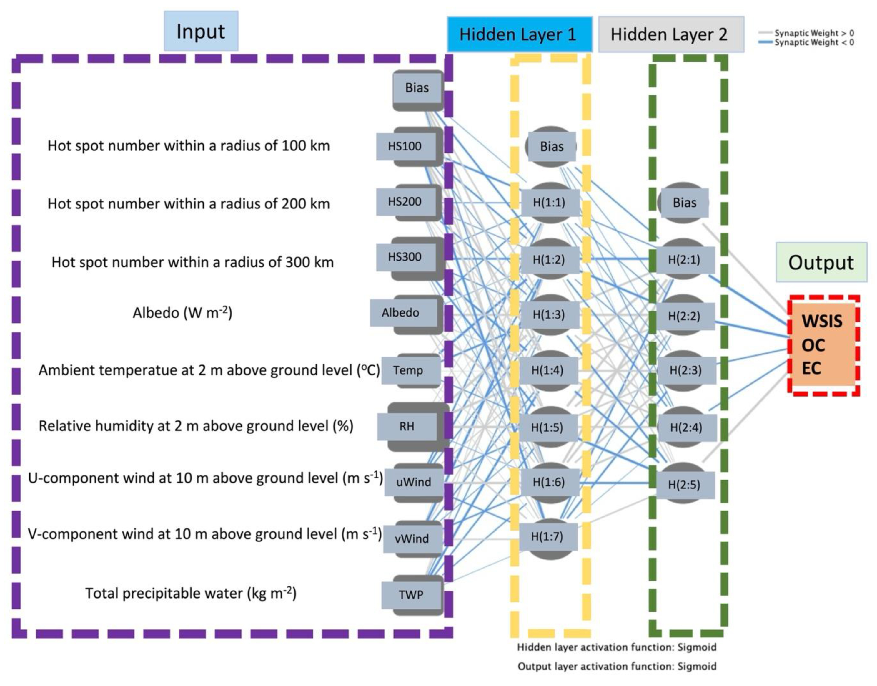
2.4.2. Artificial Neural Networks (ANNs)

ANNs, also known as simulated neural networks, are a subdivision of machine learning and are at the centre of deep learning processes [37,38]. The concept of this sophisticated algorithm was motivated by the neural network in the human brain, consisting of neurones or nerve cells that transmit and process signals received from sensory receptors. There are node layers, input payers, and hidden layers, which are the three main features of an ANN. Theoretically, an individual node, or artificial neuron, links to other nodes and has a related weight and threshold. If any singular the node is higher than the critical value, the node automatically transmits information to the next layer of the neural network. By contrast, no available information is transferred to the next layer of the neural network.

There are several benefits of using ANNs to analyse the nonlinear interrelationship between dependent and independent variables in comparison with those of conventional regression analysis, such as multinomial logistic regression, linear mixed models, and nonlinear regression. It is well-known that these complicated variants of regression analysis are impractical in real-world situations to exemplify the importance of input variables over their outcomes. As ANNs are statistical techniques that involve a large number of correlated nodes frequently called ‘neurones’, this mathematical algorithm can be applied to clarify nonlinear system functions [39,40]. The multilayer perceptron (MLP) is acknowledged as an FNN, which is the easiest type of ANN devised where the data transfer in only one direction, forward, from the input nodes, through the hidden nodes (if any), and to the output nodes [38]. In this study, MLP was employed because of its comparatively powerful training steps combined with the requirement of optimising the weights of the artificial layers of neurones [41,42]. In spite of the fact that several potential contributors, such as vehicle exhausts, factory emissions, open burnings, and domestic heating, are responsible for the altering contents of WSIS, OC, and EC ([1,21,22]), weather conditions can dramatically affect the fluctuations of these chemical constituents [43,44,45].

To assess the influence of the meteorological parameters on the particulate contents of the selected 12 chemical constituents (i.e., TC, OC, EC, Cl⁻, NO₂⁻, NO₃⁻, SO₄²⁻, Na⁺, NH₄⁺, K⁺, Mg²⁺, and Ca²⁺) over a one-year period, the importance of independent variables was computed by applying the concept of ANNs. An illustration of a double-layer ANN (DLA) with a nonlinear sigmoid transfer function in the two hidden layers and a linear function in the output layer is shown in Figure 2. The neurones in the input layer were hotspots within radii of 100, 200, and 300 km (HS100, HS200, and HS300, respectively); albedo (W m⁻²); Temp at 2 m above ground level (°C); RH at 2 m above ground level (%); u-component wind (uWind: the u wind is parallel to the x axis) at 10-axis) at 10 m above the ground level (m s⁻¹), and total precipitable water (TWP) (kg m⁻²). The neurones in the input layer are entirely connected to those in the two hidden and output layers [46]. The previously discussed variables (i.e., the input-layered neurones) were carefully chosen as the ‘covariates’, while the particulate content of individual chemical m above the ground level (m s⁻¹), v-component wind (vWind: the v wind is parallel to the yconstituents was subsequently selected as the ‘dependent parameter’. Theoretically, any statistical simulation with a finite number of discontinuities can be predicted using a DLA with a nonlinear sigmoid transfer function in the hidden layer and a linear function in the output layer [47]. In addition, a double-layer perceptron, which is a class of FNN, was applied in this study. It is also crucial to note that hyperparameter optimization (HPO), which is a mathematical algorithm for automatically finding a search space of potential hyperparameters [48,49]. Since all numerical computations were conducted with the assistance of IBM SPSS Statistics v. 25, HPO was conducted based on numerous options (multilayer perceptron), such as user-missing values, stop training rules, the maximum steps without a decrease in error, maximum training time, and maximum training epochs. The number of hidden layers and neurons in each hidden layer was changing by one, and the performance of the SPSS HPO was detected. This statistical process decreased the risk of memorization instead of generalisation of the correlations within the concerned data set. The optimal ANN turned out to be [10-8-6-1]. Two hidden layers with two sigmoid neurons in each of them from the application of IBM SPSS Statistics v. 25.

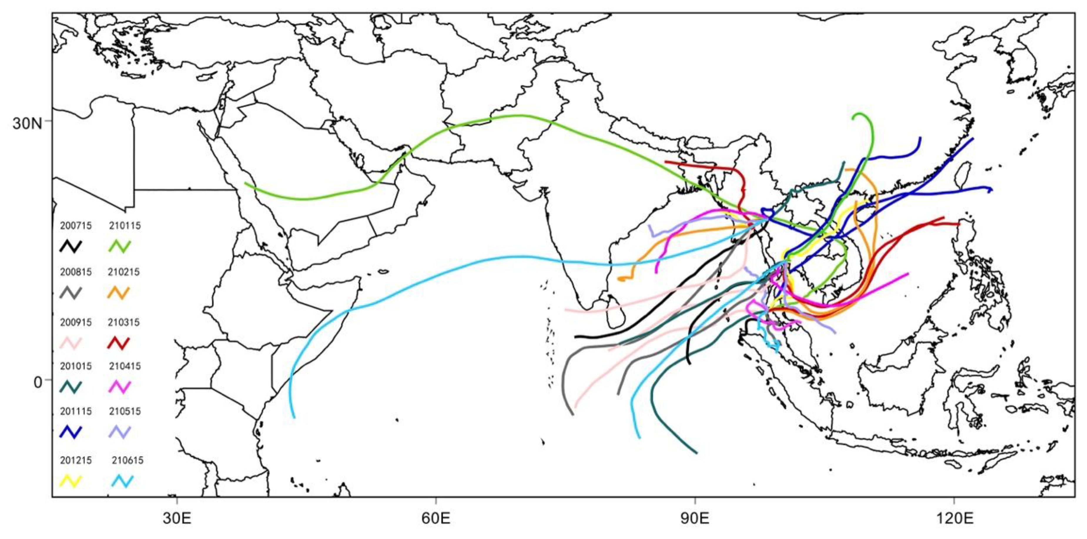
2.5. Back Trajectory Analysis and Meteorological Parameters

The Hybrid Single-Particle Lagrangian Integrated Trajectory (HYSPLIT, version 4.2.0) model developed by the NOAA Air Resources Laboratory [50] was used to calculate the five-day backward trajectories at the three sampling sites, COS (18.59° N, 98.47° E), BOS (13.78° N, 100.51° E), and POS (7.89° N, 98.35° E), at the surface level on the 15 day of each month from July 2020 to June 2021 (Figure 3). The meteorological input for the HYSPLIT model used Global Data Analysis System meteorological data with a horizontal resolution of 1° × 1°. The general climatic conditions of Thailand are influenced by two monsoon winds; the southwest monsoon and northeast monsoon. As illustrated in Figure 3, the northeast monsoon, which normally begins in October, brings low temperature and low RH from the anticyclone in mainland China. In contrast, the southwest monsoon, which generally starts in May, brings comparatively high temperature and high RH air masses from the Indian Ocean toward Thailand, resulting in high precipitation over the country. Near real-time fire products were generated approximately within 3 h of satellite observation using the Visible Infrared Imaging Radiometer Suite, which is a hotspot detector provided by the Raytheon Company onboard the polar-orbiting Suomi National Polar-orbiting Partnership and NOAA-20 weather satellites (https://firms.modaps.eosdis.nasa.gov/download/, accessed on 13 April 2022). The goal of the Global Land Data Assimilation System (GLDAS) is to incorporate satellite- and ground-based observational data products using advanced land surface modelling and data assimilation techniques to generate optimal fields of land surface states and fluxes [51]. GLDAS was used to quantify albedo (reflective quality of the Earth’s surface) (https://developers.google.com/earth-engine/datasets/catalog/NASA_GLDAS_V021_NOAH_G025_T3H#bands, accessed on 13 April 2022). Other climate variables were obtained using the Global Forecast System (GFS), a National Centres for Environmental Prediction weather forecast model that generates wind speed, RH, Temp, and soil moisture data. GFS constructs four environmental compartments (air, ocean, terrestrial soil, and sea ice) that work simultaneously to accurately predict the weather parameters (https://developers.google.com/earth-engine/datasets/catalog/NOAA_GFS0P25#bands, accessed on 13 April 2022).

2.6. Computation of Secondary Organic Carbon (SOC)

To evaluate the influence of traffic releases, biomass combustions, long-range atmospheric transport (LRAT), and photochemical decomposition on the atmospheric fluctuation of carbonaceous aerosols, the SOC was calculated from the three minimum OC/EC ratios, while the EC was used as the primary organic carbon [52,53,54], as shown in Equation (1):

$$SOC=O{C}_{total}-EC\times {\left(\frac{OC}{EC}\right)}_{pri}$$

(1)

where OC_total explains the concentration of the total OC and (OC/EC)_pri is the average value of the three minimum OC/EC ratios. Earlier studies reported that numerous factors, such as vehicle exhausts, agricultural waste burning, photochemical reactions, and the atmospheric lifetime of aerosols can dramatically alter the percentage contribution of SOC [55,56,57,58].

3. Results and Discussion

3.1. Statistical Descriptions of PM_2.5 Bounded Chemical Species

Statistical descriptions of particulate TC, OC, organic matter (OM), EC, total carbonaceous aerosol (TCA), and WSIS collected at COS, BOS, and POS are shown in

Table 1. Statistical description of the TC, OC, EC, OM. TCA, and WSIS in PM_2.5 (µg m⁻³) collected during COS, BOS, and POS.

	COS (n = 82)				BOS (n = 48)				POS (n = 61)				BOS/COS	BOS/POS	ANOVA Test
	Aver	Stdev	Min	Max	Aver	Stdev	Min	Max	Aver	Stdev	Min	Max			(p < 0.001)
TC	57	42	5.4	208	97	52	21	234	13	7.6	5.1	49	1.7	7.2	S
OC	43	31	4.9	154	71	39	18	164	11	6.0	5.1	41	1.6	6.2	S
OM	69	50	8.0	246	113	62	28	262	18	10	8.1	66	1.6	6.2	S
EC	14	12	0.45	55	26	15	3.3	71	2.0	1.8	0.064	8.3	1.9	13	S
TCA	83	51	8.4	301	140	64	32	332	20	10	8.2	74	1.7	6.9	S
Cl−	0.076	0.084	0.023	0.56	0.19	0.32	0.058	2.22	0.078	0.056	0.028	0.26	2.5	2.4	S
NO2−	0.032	0.016	N.D.	0.10	0.048	0.037	0.014	0.19	0.030	0.022	0.011	0.12	1.5	1.6	S
NO3−	0.22	0.15	0.068	0.71	1.1	0.68	0.25	4.5	0.10	0.050	0.059	0.29	5.0	11	S
SO42−	0.92	1.0	0.075	5.6	2.2	1.1	0.36	6.4	0.25	0.25	0.090	1.7	2.4	9.0	S
Na+	0.49	0.18	0.17	1.1	0.85	0.25	0.49	2.3	0.37	0.055	0.29	0.53	1.7	2.3	S
NH4+	0.18	0.27	0.023	1.5	0.49	0.43	0.0069	1.9	0.020	0.041	N.D.	0.31	2.7	24	S
K+	0.14	0.15	N.D.	0.59	0.36	0.23	0.012	1.0	0.015	0.028	N.D.	0.17	2.5	23	S
Mg2+	0.084	0.045	0.021	0.35	0.078	0.023	0.042	0.16	0.042	0.016	N.D.	0.071	0.90	1.8	S
Ca2+	0.40	0.21	N.D.	1.2	0.43	0.11	0.21	0.71	0.13	0.057	N.D.	0.23	1.1	3.4	S

Note that “N.D.” and “S” stand for “not determined” and “significant”, respectively.

. TCA was computed as the sum of the EC and OM, while the OM was calculated by multiplying the OC by 1.6 (for the urban atmosphere) [59,60].

It is worth mentioning that Thailand’s Centre for COVID-19 Situation Administration (CCSA) has agreed to launch policies including lockdown and restriction measures taken in order to limit the spread of COVID-19 that has brought rapid and ‘unprecedented’ improvements in air quality in Chiang-Mai, Bangkok, and Phuket. ANOVA was employed to compare the averages of the carbonaceous constituents and WSIS collected at the three air quality observatory sites. Significant differences (p < 0.001) were observed for all chemical species. As the diagnostic binary ratios of BOS/COS and BOS/POS for most chemical species were greater than 1, it appears reasonable to interpret these findings as a consequence of an excessively congested mass of vehicles in Bangkok. These results support previous findings, indicating that vehicle exhausts are among the major contributors of carbonaceous aerosols and WSIS in the ambient air of Bangkok [9,21,61,62,63].

It is also crucial to note that all diagnostic binary ratios of BOS/POS were generally greater than those of BOS/COS. The higher the BOS/POS ratio, the lower the emission source strength of PM_2.5 in Phuket City. Rapid industrialisation coupled with urbanisation in Bangkok in the middle of the 1980s accelerated traffic congestion. As a result, greater releases of PM_2.5 bounded carbonaceous aerosols and WSIS occurred, which subsequently led to greater concentrations in the ambient air, resulting in BOS/COS and BOS/POS diagnostic binary ratios of >1. Despite some distinctions in topographical and meteorological constraints, the chemical profiles of all three air quality observatory sites had similarities. First, the decreasing order of the particulate carbonaceous fractions observed at all sites was TCA > OM > TC > OC > EC. The lowest EC content was consistent with those of previous studies conducted in the Indo-Gangetic Plain [64], foothills of the NE Himalaya [65], Chiang-Mai [1], Bangkok [21], Hat-Yai [62], and Phuket [22]. Second, SO₄²⁻ had the highest content among the nine WSISs detected in both the COS and BOS. It is well-known that SO₄²⁻ is the dominant WSIS in PM_2.5, causing haze formation and affecting the regional climate. A previous study conducted in Hangzhou, East China, from September 2015 to October 2016, found that the main sources of SO₄²⁻ were coal combustion, vehicle exhausts, and oil consumption, which contributed 85.5%, 12.8%, and 1.7%, respectively [66].

It is worth mentioning that the Mae Moh Lignite Power Plant (MMLPL), which is located approximately 140 km SE of COS, has been operating since 1972 and consists of three units, each of 75 MW. In 2022, the MMLPL was enlarged to enhance its capacity from over 100,000 tonne daily to a million tonnes with its current power generators of 14 units. Hence, it appears reasonable to assume that coal combustion and traffic emissions are the two principal sources of particulate SO₄²⁻ in the ambient air of Chiang-Mai. In addition, the highest contents of Na⁺ detected at POS underline the importance of maritime aerosols as one of the main contributors of PM_2.5 in Phuket.

3.2. Spatial and Temporal Distribution of OC/EC Ratios and SOC

Over the past few decades, the diagnostic binary ratio of OC/EC has been widely applied in the source apportionment of carbonaceous aerosols [67,68]. The average OC/EC ratios obtained from this study were 3.49 ± 1.17, 2.86 ± 0.832, and 10.1 ± 11.3 for COS, BOS, and POS, respectively (

Table 2. Statistical descriptions of the OC/EC ratios and SOC in PM_2.5 collected at COS, BOS, and POS.

	OC/EC		The Three Lowest OC/EC		SOC (μg m−3)		SOC (%)
	Aver	Stdev	Aver	Aver	Aver	Stdev	Aver	Stdev
COS	3.49	1.17	2.24	0.142	12.4	8.92	31.4 15.2
BOS	2.86	0.832	1.76	0.127	25.0	18.2	34.3 16.1
POS	10.1	11.3	3.10	0.150	5.35	2.38	53.2 23.9

). The comparatively low OC/EC ratio with 29% of standard deviation detected at BOS was in good agreement with the heavy traffic congestion in Bangkok owing to the extremely low automobile speed during peak rush hour periods with 8.1 km h⁻¹ and 11.4 km h⁻¹ for trunk roads and expressways, respectively [69]. This value (2.86) is comparable to those of previous studies conducted in urban areas, such as the heavy traffic roadside in Xi’an, China (3.2) [70]. However, it is crucial to note that several studies including tunnel experiments report the much lower traffic related OC/EC ratios within the 0.3 to 0.4 range [67,71]. This can be explained by many plausible factors responsible for the elevated OC/EC ratio, particularly in the heavy traffic urban areas of Bangkok. First, recent studies have noted that biomass burning is the second largest source of PM_2.5 in ambient air in Chiang-Mai, Bangkok, and Phuket [1,21,22]. These source apportionment results are consistent with a recent report suggesting that 83% of total crop residue combustion in Thailand comes from rice and sugarcane [72]. It is well-known that biomass burning can cause relatively high OC/EC ratios in PM_2.5 [73]. Second, the magnitude of photochemical decomposition in a tropical atmosphere can accelerate the oxidation of elemental carbon and thus increase the OC/EC ratios in PM_2.5 [74,75,76].

Based on earlier research on OC and EC measured at COS, BOS, and POS from March 2017 to February 2018, the percentage contributions of SOC to OC_total were calculated as 46.6%, 36.3%, and 47.5%, respectively [1,21,22]. The minimum proportional contribution of SOC detected at BOS from March 2017 to February 2018 (36.3%; [21]) and from July 2020 to June 2021 (34.3%; this study) highlight the significance of vehicle releases as one of the major sources of PM_2.5. These results are consistent with those of earlier studies showing that traffic emissions are the largest potential contributor of PM_2.5 in the ambient air of Bangkok [21,63,77,78,79,80]. A similar pattern was observed in the present study, with the highest percentage contribution of SOC detected at POS at a value of 53.2%, as illustrated in Table 2. As there was no transboundary haze from Kalimantan, Indonesia, and Malaysia during the observation period, it appears reasonable to interpret the comparatively high SOC detected at POS as a consequence of the LRAT of maritime aerosols.

Further attempts to investigate the impact of biomass burning on the elevation of particulate chemical species were conducted by classifying the dataset into two groups: non-haze (i.e., a period during which HS-100 is less than 10 hotspots) and haze periods (a period during which HS-100 is greater than 10 hotspots), as displayed in

Table 3. Statistical description of carbonaceous aerosols and WSIS in PM_2.5 collected at COS, BOS, and POS during the non-haze and haze episodes.

		TC	OC	EC	Cl−	NO2−	NO3−	SO42−	Na+	NH4+	K+	Mg2+	Ca2+
Non-Haze *	Aver	21	17	4.6	0.090	0.030	0.15	0.36	0.42	0.037	0.036	0.055	0.21
	Stdev	16	12	5.0	0.088	0.020	0.20	0.43	0.16	0.072	0.061	0.027	0.15
	Count	103	103	103	103	103	103	103	103	103	103	103	103
Haze **	Aver	91	68	23	0.12	0.04	0.69	1.8	0.69	0.41	0.30	0.086	0.45
	Stdev	49	36	14	0.24	0.03	0.65	1.2	0.27	0.40	0.21	0.041	0.19
	Count	88	88	88	88	88	88	88	88	88	88	88	88
Haze/Non-Haze		4.3	4.0	5.1	1.4	1.4	4.5	5.0	1.6	11	8.2	1.6	2.1
	T-test (p < 0.05)	S	S	S	NS	S	S	S	S	S	S	S	S

* A non-Haze episode can be defined as a period that HS-100 is less than 10 hotspots; ** Haze episodes can be defined as a period that HS-100 is larger than 10 hotspots.

. Significant increases in the atmospheric concentrations of all chemical species, except Cl⁻, were detected during the haze episode. This indicates the influence of forest fires and/or open agricultural waste burning on the enhancement of both carbonaceous aerosols and the WSIS. To evaluate the impact of the hotspot number on the increase in particulate chemical constituents, the haze/non-haze ratio was carefully analysed. Generally, the higher the haze/non-haze ratio, the greater the effect of biomass burning on the enhancement of atmospheric chemical concentrations. Exceedingly high haze/non-haze ratios were detected for NH₄⁺ and K⁺ with values of 11 and 8.2, respectively. Ammonia pollution from farming has been widely studied in various agricultural areas, raising public concern over its potential adverse human health impacts [81]. As agricultural waste burning accelerates the NH₃ emission rates from mineral fertiliser application and livestock, future air pollution mitigation measures must acknowledge the capability of decreasing NH₃ release, particularly in crop planting areas and cultivation zones. The remarkably high haze/non-haze ratio of K⁺ highlights the potential of applying WSIS as a chemical tracer for identifying biomass burning in source apportionment models. This interpretation is in accordance with previous studies that used K⁺ as a biomarker for tracing the impact of crop residue burning in receptor models [82,83,84].

3.3. Pearson Correlation Coefficients (PCCs) and PCA

PCCs provide some unique features that can be used to analyse the impact of weather conditions on the variation in the atmospheric contents of chemical species. The four different patterns of PCCs are shown in

Table 4. Pearson correlation coefficients of meteorological parameters and chemical species in PM_2.5 collected at COS, BOS, and POS. Any values that higher than 0.5 and lower than −0.5 will be highlighted as bold.

	HS-100	HS-200	HS-300	Albedo	Temp	RH	u-Wind	v-Wind	TWP	TC	OC	EC	Cl−	NO2−	NO3−	SO42−	Na+	NH4+	K+	Mg2+	Ca2+
HS-100	1.00
HS-200	0.95	1.00
HS-300	0.88	0.98	1.00
Albedo	−0.29	−0.33	−0.36	1.00
Temp	−0.09	−0.06	−0.06	0.36	1.00
RH	−0.56	−0.63	−0.65	0.39	−0.30	1.00
u-Wind	0.03	0.01	−0.01	0.26	0.13	0.10	1.00
v-Wind	0.06	0.12	0.18	−0.36	0.34	−0.25	0.17	1.00
TWP	−0.47	−0.54	−0.57	0.63	0.50	0.57	0.28	−0.03	1.00
TC	0.39	0.47	0.50	−0.51	−0.02	−0.73	−0.20	0.20	−0.60	1.00
OC	0.40	0.47	0.51	−0.51	−0.04	−0.73	−0.20	0.19	−0.61	1.00	1.00
EC	0.37	0.45	0.48	−0.51	0.02	−0.72	−0.19	0.23	−0.55	0.98	0.96	1.00
Cl−	−0.04	−0.03	−0.02	−0.02	0.20	−0.07	−0.03	0.27	0.05	0.16	0.19	0.09	1.00
NO2−	0.12	0.18	0.19	−0.05	0.10	−0.30	−0.08	0.10	−0.15	0.31	0.31	0.30	0.17	1.00
NO3−	0.05	0.13	0.17	−0.28	0.29	−0.53	−0.20	0.28	−0.19	0.75	0.73	0.77	0.23	0.36	1.00
SO42−	0.26	0.40	0.46	−0.40	0.26	−0.72	−0.15	0.37	−0.41	0.80	0.78	0.82	0.10	0.33	0.72	1.00
Na+	0.05	0.12	0.17	−0.34	0.38	−0.52	−0.15	0.48	−0.15	0.60	0.60	0.58	0.64	0.32	0.66	0.67	1.00
NH4+	0.27	0.40	0.46	−0.34	0.17	−0.66	−0.14	0.25	−0.41	0.82	0.80	0.85	0.04	0.34	0.77	0.94	0.55	1.00
K+	0.29	0.39	0.43	−0.43	0.11	−0.71	−0.20	0.25	−0.48	0.95	0.95	0.94	0.31	0.36	0.82	0.85	0.72	0.86	1.00
Mg2+	0.10	0.14	0.16	−0.37	−0.08	−0.23	−0.07	0.19	−0.24	0.40	0.40	0.37	0.31	0.10	0.27	0.44	0.50	0.34	0.41	1.00
Ca2+	0.17	0.25	0.30	−0.55	−0.05	−0.44	−0.13	0.33	−0.40	0.61	0.61	0.60	0.20	0.18	0.44	0.66	0.55	0.55	0.59	0.82	1.00

. First, some considerably strong negative correlation coefficients between the hotspot number and ambient temperature implied that fires tend to occur when weather conditions are dry, particularly in cold periods. Numerous studies have reported the air quality deterioration of northern administrative provinces as triggered by wildfires, especially in winter [1,9,61,85]. Second, some fairly strong negative correlation coefficients of RH vs. TC (−0.73), RH vs. SO₄²⁻ (−0.72), RH vs. NH₄⁺ (−0.66), and RH vs. K⁺ (−0.71) suggest that dry weather conditions in the cold period played a crucial role in governing the atmospheric contents of these chemical species. The remarkably strong negative correlation between RH and K⁺ highlights the importance of WSIS as a geochemical tracer of crop residue burning, which is in good agreement with previous studies [82,83,84]. Third, some appreciably strong negative correlation coefficients for TWP vs. TC (−0.60), TWP vs. OC (−0.61), and TWP vs. EC (−0.55) underline the significance of wet deposition as one of the main depletion mechanisms of carbonaceous aerosols in ambient air. Fourth, some exceedingly strong positive correlation coefficients (>0.80) of SO₄²⁻, Na⁺, NH₄⁺, and K⁺ revealed the possibility of having similar potential sources.

In this study, PCA was applied to further quantify the probable sources of particulate WSIS and carbonaceous aerosols. This advanced statistical technique is based on the hypothesis that the period for which PM_2.5 will remain in the ambient air of a monitoring station will hypothetically be the same for target chemicals from the same source. The target chemicals were chemically analysed in a comparatively large number of air samples from a single station over the monitoring period. It is crucial to note that each factor is assumed to be profoundly related to the contributor type. The five major principal components of the 12 selected chemical species coupled with nine meteorological parameters demonstrated interesting results associated with the potential contributors of PM_2.5 in the ambient air of Thailand (

Table 5. Principal component analysis of the meteorological parameters and chemical species in PM_2.5 obtained from this study.

	Principal Component (PC)
	PC1	PC2	PC3	PC4	PC5
HS−100	0.105	0.947	0.040	0.007	−0.001
HS−200	0.209	0.959	0.072	0.008	0.023
HS−300	0.260	0.927	0.109	0.009	0.033
Albedo	−0.281	−0.261	−0.701	0.088	0.209
Temp	0.274	−0.125	−0.383	0.309	0.697
RH	−0.673	−0.549	−0.072	−0.105	−0.109
u−Wind	−0.216	0.089	−0.032	−0.194	0.645
v−Wind	0.184	0.072	0.398	0.190	0.622
TWP	−0.325	−0.530	−0.408	0.118	0.480
TC	0.858	0.295	0.282	0.088	−0.153
OC	0.836	0.306	0.289	0.112	−0.172
EC	0.888	0.261	0.258	0.025	−0.102
Cl−	0.002	−0.049	0.217	0.886	0.081
NO2−	0.355	0.152	−0.185	0.461	−0.138
NO3−	0.877	−0.083	0.059	0.219	0.048
SO42−	0.866	0.187	0.260	0.069	0.168
Na+	0.578	−0.028	0.340	0.631	0.210
NH4+	0.907	0.186	0.139	−0.013	0.062
K+	0.888	0.191	0.237	0.240	−0.071
Mg2+	0.214	−0.002	0.762	0.247	0.049
Ca2+	0.462	0.077	0.756	0.115	0.056
%Total of Variance	45.5	14.1	9.10	7.34	5.04

Extraction Method: Principal Component Analysis. Varimax Rotation converged in 9 iterations.

). Strong positive correlations (>0.80) among TC, OC, EC, NO₃⁻, SO₄²⁻, NH₄⁺, and K⁺ were detected in PC1 for all three air quality observatory sites. As K⁺ and NH₄⁺ are broadly applied as indicators of biomass burning and ammonium nitrate fertiliser release, as previously discussed, it seems rational to interpret PC1 as agricultural waste combustion with a percentage contribution of 46%. A moderately strong negative correlation coefficient of RH (−0.67) observed in PC1 suggested that TC, OC, EC, NO₃⁻, SO₄²⁻, NH₄⁺, and K⁺ were released into the atmosphere during dry climate conditions in winter. As the majority of hotspots (>90%) were detected in reserved forests and protected areas, it appears reasonable to ascribe extremely strong positive correlation coefficients (>0.90) for HS−100, HS−200, and HS−300 coupled with considerably low correlation coefficients of RH and TWP (<−0.5) as a consequence of wildfires in forestry restricted areas with a proportional contribution of 14%. Strong positive correlation coefficients of Na⁺ and Cl⁻ measured in PC4 revealed substantial effects of maritime aerosols, with a percentage contribution of 7.3%. It is also interesting to note that Mg²⁺ and Ca²⁺ were deeply connected with the solar reflectivity (i.e., albedo), probably due to their chemical capability as cloud condensation nuclei (CCNs), which are hygroscopic, meaning that they attract water molecules.

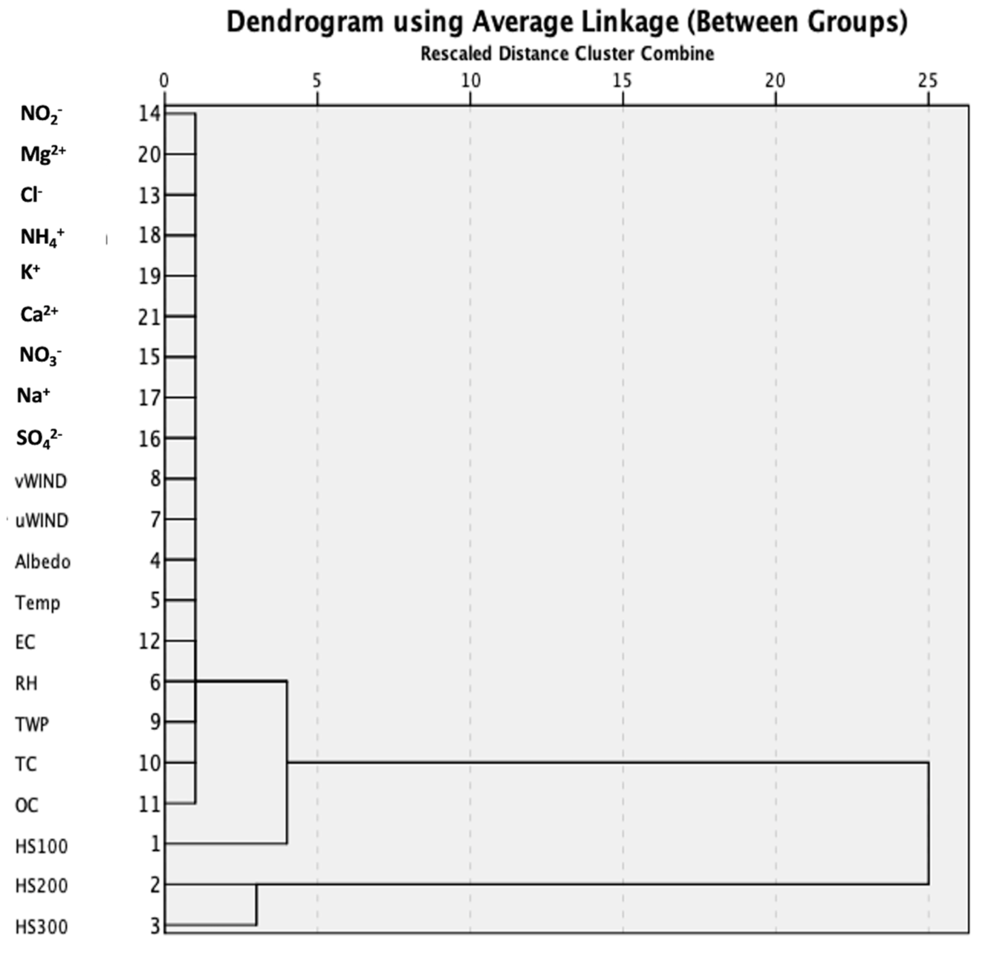
3.4. Hierarchical Cluster Analysis (HCA) and ANNs of Chemical Species in PM_2.5

To increase the credibility of the mathematical models and create higher prediction accuracies, ~70% of the detected data were employed for training, and the remaining 30% were used for model validation (

Table 6. The case processing summary and independent variable importance using an artificial neural network.

Case Processing Summary	TC	OC	EC	OC/EC	Cl−	NO2−	NO3−	SO42−	Na+	NH4+	K+	Mg2+	Ca2+
	%	%	%	%	%	%	%	%	%	%	%	%	%
ANNs-Training	68.1	67.5	73.8	73.8	71.7	63.9	66.5	71.2	73.8	72.8	70.7	69.6	65.4
Measured Data-Testing	31.9	32.5	26.2	26.2	28.3	36.1	33.5	28.8	26.2	27.2	29.3	30.4	34.6
Valid	100	100	100	100	100	100	100	100	100	100	100	100	100
Model Summary
Training-Sum of Squares Error	1.17	0.898	0.749	0.686	0.507	0.704	0.613	0.564	0.530	0.996	0.830	0.515	0.728
Training—Relative Error	0.362	0.281	0.249	0.928	0.899	0.913	0.295	0.272	0.477	0.548	0.312	0.510	0.437
Testing—Sum of Squares Error	0.372	0.335	0.369	0.052	0.038	0.608	1.31	0.352	0.092	0.310	0.182	0.704	0.265
Testing-Relative Error	0.290	0.197	0.472	0.791	0.894	0.954	0.595	0.335	0.355	0.374	0.228	0.731	0.324
Independent Variable Importance	%	%	%	%	%	%	%	%	%	%	%	%	%
HS-100	69.5	22.7	25.3	24.8	20.5	67.7	25.9	24.0	41.7	45.4	31.4	39.1	35.5
HS-200	23.5	66.1	67.9	33.9	14.4	49.8	21.6	56.6	22.0	28.8	42.9	34.6	13.9
HS-300	45.5	47.6	27.1	46.5	27.2	40.3	13.7	32.5	22.3	40.3	74.6	48.0	14.1
Albedo	46.4	59.5	44.1	100	4.70	13.5	10.9	37.7	69.0	32.5	32.1	100	100
Temp	10.4	11.3	24.2	51.0	38.5	41.4	24.7	41.7	78.8	35.7	16.1	56.5	37.4
RH	100	100	100	38.9	38.9	100	100	100	100	100	100	67.7	58.3
u-Wind	22.1	56.9	43.6	18.8	12.5	23.5	40.5	6.10	60.4	22.9	50.9	30.5	18.6
v-Wind	4.70	26.8	30.8	84.9	100	16.7	8.10	14.9	92.1	10.2	13.0	23.6	38.0
TWP	32.1	7.70	12.1	53.4	8.00	9.10	6.10	6.60	6.10	34.9	10.3	65.1	27.0

). Numerous statistical models have been used to explore the best combination of hidden layers and their neurones, sorting algorithms, and optimum learning speeds. Model summary of the uncertainties was displayed in

Table A3. Model summary of the uncertainties.

Model Summary		Ca2+	Mg2+	Cl−	K+	Na+	NH4+	NO3−	NO2−	SO42−	TC	OC	EC	OC/EC
Training	Sum of Squares Error	0.728	0.415	0.507	0.83	0.342	0.996	0.613	0.704	0.564	0.949	0.854	0.749	0.513
	Relative Error	0.437	0.636	0.899	0.312	0.354	0.548	0.295	0.913	0.272	0.256	0.221	0.249	0.776
	Stopping Rule Used	1 consecutive step(s) with no decrease in error a
	Training Time	0:00:00.02
Testing	Sum of Squares Error	0.265	0.152	0.038	0.182	0.174	0.31	1.31	0.608	0.352	0.852	0.87	0.369	0.102
	Relative Error	0.324	0.661	0.894	0.228	0.489	0.374	0.595	0.954	0.335	0.405	0.402	0.472	0.685

^a Error computations are based on the testing samples.

(see Appendix A). In this study, nine covariates, namely HS100, HS200, HS300, albedo, Temp, RH, uWind, vWind, and TWP, were standardised using the rescaling method (see

Table A1. Nomenclature and symbolism.

Symbol	Description
αa,532	The absorption coefficient at 532 nm
ACE1	The first aerosol characterisation experiment
ANNs	Artificial Neural Networks
ANOVA	Analysis of Variance
AQM	Air Quality Model
BOS	Bangkok Air Quality Observatory Site
Ca2+	Calcium ion
CCNs	Cloud condensation nuclei, also known as cloud seeds, are small particles typically 0.2 µm, or 1/100 the size of a cloud droplet on which water vapor condenses.
CCSA	Thailand’s Centre for COVID-19 Situation Administration
Cl−	Chloride ion
COS	Chiang-Mai Air Quality Observatory Site
EC	Elemental Carbon
ERI	Emission Reduction Impacts
FNN	Feedforward Neural Network
GFS	the Global Forecast System
GLDAS	The goal of the Global Land Data Assimilation System
HCA	Hierarchical Cluster Analysis
HS-100	Hotspots within radii of 100 km
HS-200	Hotspots within radii of 200 km
HS-300	Hotspots within radii of 300 km
HYSPLIT	The Hybrid Single-Particle Lagrangian Integrated Trajectory
INC	Incremental methods
K+	Potassium ion
Mg2+	Magnesium ion
MLP	Multilayer Perceptron
MLRA	Multiple Linear Regression Analysis
MMLPL	the Mae Moh Lignite Power Plant
MT	Mass-Transfer methods
NARIT	National Astronomical Research Institute of Thailand
NH4+	Ammonium ion
NO2	Nitrogen dioxide
NO3−	Nitrate ion
NOAA-20	NOAA-20, designated JPSS-1 prior to launch, is the first of the United States National Oceanic and Atmospheric Administration’s latest generation of U.S. polar-orbiting, non-geosynchronous, environmental satellites called the Joint Polar Satellite System. NOAA-20 was launched on 18 November 2017 and joined the Suomi National Polar-orbiting Partnership satellite in the same orbit.
O3	Ozone
OC	Organic Carbon
PCA	Principal Component Analysis
PM2.5	PM2.5 describes fine inhalable particles, with diameters that are generally 2.5 μm and smaller
PMF	Positive Matrix Factorisation
POS	Phuket Air Quality Observatory Site
PSU	Prince of Songkla University
PTEF	Polytetrafluoroethylene
RH	Relative humidity
RMs	Receptor-Oriented Models
SSEs	Some squared errors
SSRU	Suan Sunandha Rajabhat University
SO2	Sulphur dioxide
SO42−	Sulphate ion
SOC	Secondary Organic Carbon
T	Ambient temperature
TC	Total Carbon
TCA	Total Carbonaceous Aerosol
TPW	Total Precipitable Water
US-EPA	United States Environmental Protection Agency
WD	Wind direction
uWind	u-component wind
vWind	v-component wind
WSIS	Water-Soluble Ionic Species

and

Table A2. Network information related to the machine learning process.

Input Layer	Covariates	1	HS-100
		2	HS-200
		3	HS-300
		4	Albedo
		5	Temp
		6	RH
		7	u-Wind
		8	v-Wind
		9	TWP
	Number of Units a		9
	Rescaling Method for Covariates		Standardized
Hidden Layer(s)	Number of Hidden Layers		2
	Number of Hidden Layer 1 a		7
	Number of Hidden Layer 2 a		5
	Activation Function		Sigmoid
Output Layer	Dependent Variables 1		Chemical Species
	Number of Units		1
	Rescaling Method for Scale Dependents		Normalized
	Activation Function		Sigmoid
	Error Function		Sum of Squares

^a Excluding the bias unit.

in Appendix A). The two hidden layers were processed using a sigmoid activation function. The output layer consisted of 12 particulate chemical species, which were standardised by rescaling with a sigmoid activation function. Some squared errors (SSEs) were carefully chosen as error functions during the training of the basic MLP neural network (Table 6). SSEs can be used to reduce the magnitude of both the positive and negative errors. Additionally, SSEs can be applied as numerical algorithms to analyse the forecasting accuracy of ANN simulations. The training and testing performance of the ANN model can also be evaluated by analysing the training and testing relative errors. The percentage contributions of the importance of the independent variables highlight the importance of each meteorological variable on the fluctuations of the 12 particulate chemical species.

RH was the most prominent factor that controlled the variation in the particulate concentrations of TC, OC, EC, NO₂⁻, NO₃⁻, SO₄²⁻, Na⁺, NH₄⁺, and K⁺ with a 100% independent variable importance. This indicates that wet deposition is one of the most effective scavenging mechanisms for carbonaceous aerosols and particulate WSIS in tropical atmospheres. The ANN simulations were in accordance with the HCA dendrogram, as illustrated in Figure 4. NO₂⁻, Mg²⁺, Cl⁻, NH₄⁺, K⁺, Ca²⁺, NO₃⁻, Na⁺, and SO₄²⁻ leaves were more similar to each other and close to RH than they were to HS100, HS200, and HS300 leaves. This indicates that rainfall is substantially connected with the depletion mechanism of all WSIS, whereas hotspot numbers can be considered as major sources of carbonaceous aerosols. The albedo (i.e., solar reflectivity) was the second greatest covariate governing the alteration of the OC/EC ratio, Mg²⁺, and Ca²⁺ with 100% independent variable importance. Again, the results of the ANN models were consistent with the results of the HCA dendrogram, showing that Mg²⁺ and Ca²⁺ leaves were much closer to albedo than to HS100, HS200, and HS300 leaves. Although calcium- and magnesium-containing salts are crucial components of mineral dust and maritime aerosols, little is known about their physicochemical properties. The most recent study on eight Ca- and Mg-containing salts, including Ca(NO₃)₂·4H₂O, Mg(NO₃)₂·6H₂O, MgCl₂·6H₂O, CaCl₂·6H₂O, Ca(HCOO)₂, Mg(HCOO)₂·2H₂O, Ca(CH₃COO)₂·H₂O, and Mg(CH₃COO)₂·4H₂O, showed hygroscopic properties as a function of RH [85]. As the hygroscopicity of pre-existing aerosol particles, and concentrations of condensable gases can also affect the optical thickness and reflectance of clouds [86], the 100% independent variable importance of Ca²⁺ and Mg²⁺ signified the contribution of these two WSIS as CNNs for cloud formation, thus subsequently leading to their association with albedo.

4. Conclusions

Wildfires and crop residue combustions have been the main contributors to air quality deterioration over the past few years. Source apportionment analysis, performed by the PCA model, revealed that agricultural waste burning and wildfires in restricted forest areas were the two main contributors of PM_2.5, with a percentage contribution of 46% and 14%, respectively. Therefore, mitigation strategies for reducing air pollution need to pay more attention to crop residue burning; thus, clean air-oriented agricultural policies and programmes are crucial. Numerous economic incentives, such as tax cuts and subsidies to promote non-agricultural burning products, tax rebates for investing in post-harvest machinery (e.g., sugarcane cutting machines), non-agricultural burning subsidies, and negative economic incentives for punishing open agricultural burners, should be documented in the environmental quality management plan under Section 35 of the promotion and conservation of the National Environmental Quality Act (‘NEQA’) B.E. 2535. Although significant increases in most chemical species were observed during the haze episode, the results of ANNs coupled with HCA indicated that wet deposition is one of the major scavenging mechanisms of particulate WSIS and carbonaceous aerosols. The albedo showed 100% independent variable importance for Ca²⁺ and Mg²⁺, indicating that these two WSIS can be considered as CNNs owing to their comparatively strong hygroscopicity.

References

1. Choochuay, C.; Pongpiachan, S.; Tipmanee, D.; Deelaman, W.; Iadtem, N.; Suttinun, O.; Wang, Q.; Xing, L.; Li, G.; Han, Y.; et al. Effects of Agricultural Waste Burning on PM2.5-Bound Polycyclic Aromatic Hydrocarbons, Carbonaceous Compositions, and Water-Soluble Ionic Species in the Ambient Air of Chiang-Mai, Thailand. Polycycl. Aromat. Compd. 2020, 43, 1–22. [Google Scholar] [CrossRef]
2. Pongpiachan, S. Diurnal variation, vertical distribution and source apportionment of carcinogenic polycyclic aromatic hydrocarbons (PAHs) in Chiang-Mai, Thailand. Asian Pac. J. Cancer Prev. 2013, 14, 1851–1863. [Google Scholar] [CrossRef] [Green Version]
3. Pongpiachan, S.; Hattayanone, M.; Cao, J. Effect of agricultural waste burning season on PM2.5-bound polycyclic aromatic hydrocarbon (PAH) levels in Northern Thailand. Atmos. Pollut. Res. 2017, 8, 1069–1080. [Google Scholar] [CrossRef]
4. Said, S.N.B.M.; Zahran, E.-S.M.M.; Shams, S. Forest Fire Risk Assessment Using Hotspot Analysis in GIS. Open Civ. Eng. J. 2017, 11, 786–801. [Google Scholar] [CrossRef]
5. Pongpiachan, S.; Paowa, T. Hospital out-and-in-patients as functions of trace gaseous species and other meteorological parameters in Chiang-Mai, Thailand. Aerosol Air Qual. Res. 2015, 15, 479–493. [Google Scholar] [CrossRef]
6. Bonnet, S.; Garivait, S. Seasonal variability of biomass open burning activities in the greater mekong sub-region. Glob. Environ. Res. 2011, 15, 31–37. [Google Scholar]
7. Dang, A.T.; Kumar, L.; Reid, M.; Mutanga, O. Fire danger assessment using geospatial modelling in Mekong delta, Vietnam: Effects on wetland resources. Remote Sens. Appl. Soc. Environ. 2021, 21, 100456. [Google Scholar] [CrossRef]
8. Towprayoon, S.; Bonnet, S.; Garivait, S.; Chidthaisong, A. Greenhouse gas and aerosol emissions from rice field and forest in the Mekong River basin sub-region. Greater Mekong Subreg. Acad. Res. Netw. 2008, 170, 163. [Google Scholar]
9. Pongpiachan, S.; Choochuay, C.; Chonchalar, J.; Kanchai, P.; Phonpiboon, T.; Wongsuesat, S.; Chomkhae, K.; Cao, J.; Thamrongthanyawong, S. Chemical characterisation of organic functional group compositions in PM2.5 collected at nine administrative provinces in Northern Thailand during the haze episode in 2013. Asian Pac. J. Cancer Prev. 2013, 14, 3653–3661. [Google Scholar] [CrossRef] [Green Version]
10. Thepnuan, D.; Chantara, S.; Lee, C.-T.; Lin, N.-H.; Tsai, Y.I. Molecular markers for biomass burning associated with the characterization of PM2.5 and component sources during dry season haze episodes in Upper South East Asia. Sci. Total Environ. 2019, 658, 708–722. [Google Scholar] [CrossRef]
11. Yabueng, N.; Wiriya, W.; Chantara, S. Influence of zero-burning policy and climate phenomena on ambient PM2.5 patterns and PAHs inhalation cancer risk during episodes of smoke haze in Northern Thailand. Atmos. Environ. 2020, 232, 117485. [Google Scholar] [CrossRef]
12. Reyes-Rodríguez, G.J.; Gioda, A.; Mayol-Bracero, O.L.; Collett, J., Jr. Organic carbon, total nitrogen, and water-soluble ions in clouds from a tropical montane cloud forest in Puerto Rico. Atmos. Environ. 2009, 43, 4171–4177. [Google Scholar] [CrossRef]
13. Quinn, P.K.; Coffman, D.J.; Kapustin, V.N.; Bates, T.S.; Covert, D.S. Aerosol optical properties in the marine boundary layer during ACE 1 and the underlying chemical and physical aerosol properties. J. Geophys. Res. 1998, 103, 16547–16563. [Google Scholar]
14. Li, L.; Chen, J.; Wang, L.; Melluki, W.; Zhou, H. Aerosol single scattering albedo affected by chemical composition: An investigation using CRDS combined with MARGA. Atmos. Res. 2013, 124, 149–157. [Google Scholar] [CrossRef]
15. Gao, S.; Zhao, H.; Bai, Z.; Han, B.; Xu, J.; Zhao, R.; Zhang, N.; Chen, L.; Lei, X.; Shi, W.; et al. Combined use of principal component analysis and artificial neural network approach to improve estimates of PM2.5 personal exposure: A case study on older adults. Sci. Total Environ. 2020, 726, 138533. [Google Scholar] [CrossRef] [PubMed]
16. Khojasteh, D.N.; Goudarzi, G.; Taghizadeh-Mehrjardi, R.; Asumadu-Sakyi, A.B.; Fehresti-Sani, M. Long-term effects of outdoor air pollution on mortality and morbidity–prediction using nonlinear autoregressive and artificial neural networks models. Atmos. Pollut. Res. 2021, 12, 46–56. [Google Scholar] [CrossRef]
17. Masood, A.; Ahmad, K. A model for particulate matter (PM2.5) prediction for Delhi based on machine learning approaches. Procedia Comput. Sci. 2020, 167, 2101–2110. [Google Scholar] [CrossRef]
18. Polezer, G.; Tadano, Y.S.; Siqueira, H.V.; Godoi, A.F.; Yamamoto, C.I.; de André, P.A.; Pauliquevis, T.; Andrade, M.d.F.; Oliveira, A.; Saldiva, P.H.N.; et al. Assessing the impact of PM2.5 on respiratory disease using artificial neural networks. Environ. Pollut. 2018, 235, 394–403. [Google Scholar] [CrossRef]
19. Cabaneros, S.M.; Calautit, J.K.; Hughes, B.R. A review of artificial neural network models for ambient air pollution prediction. Environ. Model. Softw. 2019, 119, 285–304. [Google Scholar] [CrossRef]
20. Zhao, X.; Liu, X.; Xing, Y.; Wang, L.; Wang, Y. Evaluation of water quality using a Takagi-Sugeno fuzzy neural network and determination of heavy metal pollution index in a typical site upstream of the Yellow River. Environ. Res. 2022, 211, 113058. [Google Scholar] [CrossRef]
21. Sresawasd, C.; Chetiyanukornkul, T.; Suriyawong, P.; Tekasakul, S.; Furuuchi, M.; Hata, M.; Dejchanchaiwong, R. Influence of Meteorological Conditions and Fire Hotspots on PM0. 1 in Northern Thailand during Strong Haze Episodes and Carbonaceous Aerosol Characterization. Aerosol Air Qual. Res. 2021, 21, 210069. [Google Scholar] [CrossRef]
22. Xing, L.; Li, G.; Pongpiachan, S.; Wang, Q.; Han, Y.; Cao, J.; Poshyachinda, S. Quantifying the contributions of local emissions and regional transport to elemental carbon in Thailand. Environ. Pollut. 2020, 262, 114272. [Google Scholar] [CrossRef] [PubMed]
23. U.S. EPA. EPA Quality Assurance Guidance Document: Method Compendium, Field Standard Operating Procedures for the PM2.5 Performance Evaluation Program; Revision No. 2; United States Environmental Protection Agency Office of Air Quality Planning and Standards: Washington, DC, USA, 2002.
24. U.S. EPA. EPA Quality Assurance Document: Method Compendium, PM2.5 Mass Weighing Laboratory Standard Operating Procedures for the Performance Evaluation Program; United States Environmental Protection Agency Office of Air Quality Planning and Standards: Washington, DC, USA, 1998.
25. Wang, Y.; Zhuang, G.; Tang, A.; Yuan, H.; Sun, Y.; Chen, S.; Zheng, A. The ion chemistry and the source of PM2.5 aerosol in Beijing. Atmos. Environ. 2005, 39, 3771–3784. [Google Scholar] [CrossRef]
26. Shen, Z.; Cao, J.; Arimoto, R.; Han, Z.; Zhang, R.; Han, Y.; Liu, S.; Okuda, T.; Nakao, S.; Tanaka, S. Ionic composition of TSP and PM2.5 during dust storms and air pollution episodes at Xi’an, China. Atmos. Environ. 2009, 43, 2911–2918. [Google Scholar] [CrossRef]
27. Chow, J.C.; Watson, J.G.; Pritchett, L.C.; Pierson, W.R.; Frazier, C.A.; Purcell, R.G. The dri thermal/optical reflectance carbon analysis system: Description, evaluation and applications in U.S. Air quality studies. Atmos. Environ. Part A Gen. Top. 1993, 27, 1185–1201. [Google Scholar] [CrossRef]
28. Han, Y.M.; Du, P.X.; Cao, J.J.; Posmentier, E.S. Multivariate analysis of heavy metal contamination in urban dusts of Xi’an, Central China. Sci. Total Environ. 2006, 355, 176–186. [Google Scholar]
29. Davies, T.; Fearn, T. Back to basics: The principles of principal component analysis. Spectrosc. Eur. 2004, 16, 20. [Google Scholar]
30. Fauvel, M.; Chanussot, J.; Benediktsson, J.A. Kernel principal component analysis for the classification of hyperspectral remote sensing data over urban areas. EURASIP J. Adv. Signal Process. 2009, 2009, 1–14. [Google Scholar] [CrossRef] [Green Version]
31. Deelaman, W.; Pongpiachan, S.; Tipmanee, D.; Suttinun, O.; Choochuay, C.; Iadtem, N.; Charoenkalunyuta, T.; Promdee, K. Source apportionment of polycyclic aromatic hydrocarbons in the terrestrial soils of King George Island, Antarctica. J. S. Am. Earth Sci. 2020, 104, 102832. [Google Scholar] [CrossRef]
32. Deelaman, W.; Pongpiachan, S.; Tipmanee, D.; Choochuay, C.; Iadtem, N.; Suttinun, O.; Wang, Q.; Xing, L.; Li, G.; Han, Y.; et al. Source identification of polycyclic aromatic hydrocarbons in terrestrial soils in Chile. J. S. Am. Earth Sci. 2020, 99, 102514. [Google Scholar] [CrossRef]
33. Deelaman, W.; Pongpiachan, S.; Tipmanee, D.; Choochuay, C.; Suttinun, O.; Charoenkalunyuta, T.; Promdee, K. Ecotoxicological risk and health risk characterization of polycyclic aromatic hydrocarbons (PAHs) in terrestrial soils of King George Island, Antarctica. Polar Sci. 2021, 29, 100715. [Google Scholar] [CrossRef]
34. Pongpiachan, S. Discrimination of the geographical origins of rice based on polycyclic aromatic hydrocarbons. Environ. Geochem. Health 2021, 44, 1619–1632. [Google Scholar] [CrossRef] [PubMed]
35. Pongpiachan, S.; Jearanaikoon, N.; Thumanu, K.; Pradubsri, J.; Supruangnet, R.; Tharasawatpipat, C.; Hashmi, M.Z.; Apiratiku, R. Using Synchrotron Radiation X-ray Fluorescence (SRXRF) to Assess the Impacts of Shipping Emissions on the Variations of PM10-bound Elemental Species. Aerosol Air Qual. Res. 2021, 21, 210030. [Google Scholar] [CrossRef]
36. Tipmanee, D.; Deelaman, W.; Pongpiachan, S.; Schwarzer, K.; Sompongchaiyakul, P. Using Polycyclic Aromatic Hydrocarbons (PAHs) as a chemical proxy to indicate Tsunami 2004 backwash in Khao Lak coastal area, Thailand. Nat. Hazards Earth Syst. Sci. 2012, 12, 1441–1451. [Google Scholar] [CrossRef]
37. Choi, R.Y.; Coyner, A.S.; Kalpathy-Cramer, J.; Chiang, M.F.; Campbell, J.P. Introduction to machine learning, neural networks, and deep learning. Transl. Vis. Sci. Technol. 2020, 9, 14. [Google Scholar]
38. Schmidhuber, J. Deep Learning in Neural Networks: An Overview. Neural Netw. 2015, 61, 85–117. [Google Scholar] [CrossRef] [Green Version]
39. Civco, D.L. Artificial neural networks for land-cover classification and mapping. Geogr. Inf. Syst. 1993, 7, 173–186. [Google Scholar] [CrossRef]
40. Kang, H.-Y.; Rule, R.; Noble, P. Artificial Neural Network Modeling of Phytoplankton Blooms and its Application to Sampling Sites within the Same Estuary; Elsevier: Amsterdam, The Netherlands, 2011; pp. 161–172. [Google Scholar]
41. Haykin, S. Neural Networks: A Comprehensive Foundation, 2nd ed.; Prentice-Hall: Hoboken, NJ, USA, 1999. [Google Scholar]
42. Siqueira, H.; Boccato, L.; Attux, R.; Lyra, C. Unorgnized machines for seasonal streamflow series forecasting. Int. J. Neural Syst. 2014, 24, 1430009–1430016. [Google Scholar] [CrossRef]
43. Sonwani, S.; Saxena, P.; Shukla, A. Carbonaceous Aerosol Characterization and Their Relationship with Meteorological Parameters During Summer Monsoon and Winter Monsoon at an Industrial Region in Delhi, India. Earth Space Sci. 2021, 8, e2020EA001303. [Google Scholar] [CrossRef]
44. Švédová, B.; Kucbel, M.; Raclavská, H.; Růžičková, J.; Raclavský, K.; Sassmanová, V. Water-soluble ions in dust particles depending on meteorological conditions in urban environment. J. Environ. Manag. 2019, 237, 322–331. [Google Scholar] [CrossRef]
45. Yao, L.; Huo, J.; Wang, D.; Fu, Q.; Sun, W.; Li, Q.; Chen, J. Online measurement of carbonaceous aerosols in suburban Shanghai during winter over a three-year period: Temporal variations, meteorological effects, and sources. Atmos. Environ. 2020, 226, 117408. [Google Scholar] [CrossRef]
46. Mollalo, A.; Mao, L.; Rashidi, P.; Glass, G.E. A GIS-Based Artificial Neural Network Model for Spatial Distribution of Tuberculosis across the Continental United States. Int. J. Environ. Res. Public Health 2019, 16, 157. [Google Scholar] [CrossRef] [PubMed] [Green Version]
47. Yonaba, H.; Anctil, F.; Fortin, V. Comparing sigmoid transfer functions for neural network multistep ahead streamflow forecasting. J. Hydrol. Eng. 2010, 15, 275–283. [Google Scholar] [CrossRef]
48. Krzywanski, J. A General Approach in Optimization of Heat Exchangers by Bio-Inspired Artificial Intelligence Methods. Energies 2019, 12, 4441. [Google Scholar] [CrossRef] [Green Version]
49. Skrobek, D.; Krzywanski, J.; Sosnowski, M.; Kulakowska, A.; Zylka, A.; Grabowska, K.; Ciesielska, K.; Nowak, W. Prediction of Sorption Processes Using the Deep Learning Methods (Long Short-Term Memory). Energies 2020, 13, 6601. [Google Scholar] [CrossRef]
50. Stein, A.F.; Draxler, R.R.; Rolph, G.D.; Stunder, B.J.B.; Cohen, M.D.; Ngan, F. NOAA’s HYSPLIT Atmospheric Transport and Dispersion Modeling System. Bull. Am. Meteorol. Soc. 2015, 96, 2059–2077. [Google Scholar] [CrossRef]
51. Rodell, M.; Houser, P.R.; Jambor, U.E.A.; Gottschalck, J.; Mitchell, K.; Meng, C.J.; Toll, D. The global land data assimilation system. Bull. Am. Meteorol. Soc. 2004, 85, 381–394. [Google Scholar] [CrossRef] [Green Version]
52. Wu, C.; Yu, J.Z. Determination of primary combustion source organic carbon-to-elemental carbon (OC/EC) ratio using ambient OC and EC measurements: Secondary OC-EC correlation minimization method. Atmos. Chem. Phys. 2016, 16, 5453–5465. [Google Scholar] [CrossRef] [Green Version]
53. Cabada, J.C.; Pandis, S.N.; Subramanian, R.; Robinson, A.L.; Polidori, A.; Turpin, B. Estimating the secondary organic aerosol contribution to PM2.5 using the EC tracer method special issue of aerosol science and technology on findings from the fine particulate matter supersites program. Aerosol Sci. Technol. 2004, 38, 140–155. [Google Scholar] [CrossRef] [Green Version]
54. Castro, L.M.; Pio, C.A.; Harrison, R.M.; Smith, D.J.T. Carbonaceous aerosol in urban and rural European atmospheres: Estimation of secondary organic carbon concentrations. Atmos. Environ. 1999, 33, 2771–2781. [Google Scholar] [CrossRef]
55. Gentner, D.R.; Isaacman, G.; Worton, D.R.; Chan, A.W.H.; Dallmann, T.R.; Davis, L.; Liu, S.; Day, D.A.; Russell, L.M.; Wilson, K.R.; et al. Elucidating secondary organic aerosol from diesel and gasoline vehicles through detailed characterization of organic carbon emissions. Proc. Natl. Acad. Sci. USA 2012, 109, 18318–18323. [Google Scholar] [CrossRef] [PubMed] [Green Version]
56. Tomaz, S.; Cui, T.; Chen, Y.; Sexton, K.G.; Roberts, J.M.; Warneke, C.; Yokelson, R.J.; Surratt, J.D.; Turpin, B.J. Photochemical Cloud Processing of Primary Wildfire Emissions as a Potential Source of Secondary Organic Aerosol. Environ. Sci. Technol. 2018, 52, 11027–11037. [Google Scholar] [CrossRef] [PubMed]
57. Zhang, X.; Liu, Z.; Hecobian, A.; Zheng, M.; Frank, N.H.; Edgerton, E.S.; Weber, R.J. Spatial and seasonal variations of fine particle water-soluble organic carbon (WSOC) over the southeastern United States: Implications for secondary organic aerosol formation. Atmos. Chem. Phys. 2012, 12, 6593–6607. [Google Scholar] [CrossRef] [Green Version]
58. Zhou, S.; Wang, Z.; Gao, R.; Xue, L.; Yuan, C.; Wang, T.; Gao, X.; Wang, X.; Nie, W.; Xu, Z.; et al. Formation of secondary organic carbon and long-range transport of carbonaceous aerosols at Mount Heng in South China. Atmos. Environ. 2012, 63, 203–212. [Google Scholar] [CrossRef]
59. Cao, J.J.; Lee, S.C.; Ho, K.F.; Zhang, X.Y.; Zou, S.C.; Fung, K.; Watson, J.G. Characteristics of carbonaceous aerosol in Pearl River Delta Region, China during 2001 winter period. Atmos. Environ. 2003, 37, 1451–1460. [Google Scholar] [CrossRef]
60. Rengarajan, R.; Sarin, M.M.; Sudheer, A.K. Carbonaceous and inorganic species in atmospheric aerosols during wintertime over urban and high-altitude sites in North India. J. Geophys. Res. Earth Surf. 2007, 112, D21307. [Google Scholar] [CrossRef]
61. Boongla, Y.; Chanonmuang, P.; Hata, M.; Furuuchi, M.; Phairuang, W. The characteristics of carbonaceous particles down to the nanoparticle range in Rangsit city in the Bangkok Metropolitan Region, Thailand. Environ. Pollut. 2021, 272, 115940. [Google Scholar] [CrossRef]
62. Pongpiachan, S.; Ho, K.F.; Cao, J. Estimation of Gas-particle partitioning Coefficients (K p) of Carcinogenic polycyclic aromatic hydrocarbons in carbonaceous aerosols collected at Chiang-Mai, Bangkok and Hat-Yai, Thailand. Asian Pac. J. Cancer Prev. 2013, 14, 2461–2476. [Google Scholar] [CrossRef] [Green Version]
63. Pongpiachan, S.; Kositanont, C.; Palakun, J.; Liu, S.; Ho, K.F.; Cao, J. Effects of day-of-week trends and vehicle types on PM2.5-bounded carbonaceous compositions. Sci. Total Environ. 2015, 532, 484–494. [Google Scholar] [CrossRef]
64. Bhowmik, H.S.; Naresh, S.; Bhattu, D.; Rastogi, N.; Prévôt, A.S.; Tripathi, S.N. Temporal and spatial variability of carbonaceous species (EC.; OC.; WSOC and SOA) in PM2.5 aerosol over five sites of Indo-Gangetic Plain. Atmos. Pollut. Res. 2021, 12, 375–390. [Google Scholar] [CrossRef]
65. Rajput, P.; Sarin, M.; Kundu, S.S. Atmospheric particulate matter (PM2.5), EC, OC, WSOC and PAHs from NE–Himalaya: Abundances and chemical characteristics. Atmos. Pollut. Res. 2013, 4, 214–221. [Google Scholar] [CrossRef] [Green Version]
66. Lin, Y.-C.; Yu, M.; Xie, F.; Zhang, Y. Anthropogenic Emission Sources of Sulfate Aerosols in Hangzhou, East China: Insights from Isotope Techniques with Consideration of Fractionation Effects between Gas-to-Particle Transformations. Environ. Sci. Technol. 2022, 56, 3905–3914. [Google Scholar] [CrossRef] [PubMed]
67. Liu, B.; Yang, J.; Yuan, J.; Wang, J.; Dai, Q.; Li, T.; Bi, X.; Feng, Y.; Xiao, Z.; Zhang, Y.; et al. Source apportionment of atmospheric pollutants based on the online data by using PMF and ME2 models at a megacity, China. Atmos. Res. 2017, 185, 22–31. [Google Scholar] [CrossRef]
68. Yin, J.; Harrison, R.M.; Chen, Q.; Rutter, A.; Schauer, J.J. Source apportionment of fine particles at urban background and rural sites in the UK atmosphere. Atmos. Environ. 2010, 44, 841–851. [Google Scholar] [CrossRef]
69. Kubota, H. Bangkok-World’s Worst Traffic Jams and Their Causes. Wheel. Ext. 1996, 96, 5–9. [Google Scholar]
70. Shen, Z.; Han, Y.; Cao, J.; Tian, J.; Zhu, C.; Liu, S.; Liu, P.; Wang, Y. Characteristics of Traffic-related Emissions: A Case Study in Roadside Ambient Air over Xi’an, China. Aerosol Air Qual. Res. 2010, 10, 292–300. [Google Scholar] [CrossRef]
71. Charron, A.; Polo-Rehn, L.; Besombes, J.-L.; Golly, B.; Buisson, C.; Chanut, H.; Marchand, N.; Guillaud, G.; Jaffrezo, J.-L. Identification and quantification of particulate tracers of exhaust and non-exhaust vehicle emissions. Atmos. Chem. Phys. 2019, 19, 5187–5207. [Google Scholar] [CrossRef] [Green Version]
72. Kumar, I.; Bandaru, V.; Yampracha, S.; Sun, L.; Fungtammasan, B. Limiting rice and sugarcane residue burning in Thailand: Current status, challenges and strategies. J. Environ. Manag. 2020, 276, 111228. [Google Scholar] [CrossRef]
73. Kim, Y.; Seo, J.; Kim, J.Y.; Lee, J.Y.; Kim, H.; Kim, B.M. Characterization of PM2.5 and identification of transported secondary and biomass burning contribution in Seoul, Korea. Environ. Sci. Pollut. Res. 2018, 25, 4330–4343. [Google Scholar] [CrossRef]
74. Wang, Z.; Wang, T.; Guo, J.; Gao, R.; Xue, L.; Zhang, J.; Zhou, Y.; Zhou, X.; Zhang, Q.; Wang, W. Formation of secondary organic carbon and cloud impact on carbonaceous aerosols at Mount Tai, North China. Atmos. Environ. 2012, 46, 516–527. [Google Scholar] [CrossRef]
75. Zhang, C.; Lu, X.; Zhai, J.; Chen, H.; Yang, X.; Zhang, Q.; Zhao, Q.; Fu, Q.; Sha, F.; Jin, J. Insights into the formation of secondary organic carbon in the summertime in urban Shanghai. J. Environ. Sci. 2018, 72, 118–132. [Google Scholar] [CrossRef]
76. Zhong, M.; Jang, M. Dynamic light absorption of biomass-burning organic carbon photochemically aged under natural sunlight. Atmos. Chem. Phys. 2014, 14, 1517–1525. [Google Scholar] [CrossRef] [Green Version]
77. Oanh, N.K.; Kongpran, J.; Hang, N.; Parkpian, P.; Hung, N.; Lee, S.-B.; Bae, G.-N. Characterization of gaseous pollutants and PM2.5 at fixed roadsides and along vehicle traveling routes in Bangkok Metropolitan Region. Atmos. Environ. 2013, 77, 674–685. [Google Scholar] [CrossRef]
78. Pongpiachan, S.; Liu, S.; Huang, R.-J.; Zhao, Z.; Palakun, J.; Kositanont, C.; Cao, J. Variation in Day-of-Week and Seasonal Concentrations of Atmospheric PM2.5-Bound Metals and Associated Health Risks in Bangkok, Thailand. Arch. Environ. Contam. Toxicol. 2017, 72, 364–379. [Google Scholar] [CrossRef] [PubMed]
79. Pongpiachan, S.; Iijima, A.; Cao, J. Hazard Quotients, Hazard Indexes, and Cancer Risks of Toxic Metals in PM10 during Firework Displays. Atmosphere 2018, 9, 144. [Google Scholar] [CrossRef] [Green Version]
80. Sahanavin, N.; Tantrakarnapa, K.; Prueksasit, T. Ambient PM10 and PM2.5 concentrations at different high traffic-related street configurations in Bangkok, Thailand. Southeast Asian J. Trop. Med. Public Health 2016, 47, 528–535. [Google Scholar]
81. Stokstad, E. Ammonia Pollution from Farming May Exact Hefty Health Costs. Science 2014, 343, 238. [Google Scholar] [CrossRef]
82. Pachon, J.E.; Weber, R.J.; Zhang, X.; Mulholland, J.A.; Russell, A.G. Revising the use of potassium (K) in the source apportionment of PM2.5. Atmos. Pollut. Res. 2013, 4, 14–21. [Google Scholar] [CrossRef] [Green Version]
83. Lee, A.K.; Lau, A.P.; Cheng, J.Y.; Fang, M.; Chan, C.K. Source identification analysis for the airborne bacteria and fungi using a biomarker approach. Atmos. Environ. 2007, 41, 2831–2843. [Google Scholar] [CrossRef]
84. Yu, J.; Yan, C.; Liu, Y.; Li, X.; Zhou, T.; Zheng, M. Potassium: A Tracer for Biomass Burning in Beijing? Aerosol Air Qual. Res. 2018, 18, 2447–2459. [Google Scholar] [CrossRef] [Green Version]
85. Guo, L.; Gu, W.; Peng, C.; Wang, W.; Li, Y.J.; Zong, T.; Tang, Y.; Wu, Z.; Lin, Q.; Ge, M.; et al. A comprehensive study of hygroscopic properties of calcium- and magnesium-containing salts: Implication for hygroscopicity of mineral dust and sea salt aerosols. Atmos. Chem. Phys. 2019, 19, 2115–2133. [Google Scholar] [CrossRef] [Green Version]
86. Kulmala, M.; Korhonen, P.; Vesala, T.; Hansson, H.C.; Noone, K.; Svenningsson, B. The effect of hygroscopicity on cloud droplet formation. Tellus B Chem. Phys. Meteorol. 1996, 48, 347–360. [Google Scholar] [CrossRef]
Figure 1. Air quality observatory sites at Chiang-Mai (COS), Bangkok (BOS), and Phuket (POS).
Atmosphere 13 01042 g001
Figure 2. Feed forward neural network for PM2.5-bounded WSIS, OC, and EC predictions.
Atmosphere 13 01042 g002
Figure 3. The five-day backward trajectories arriving at the sampling locations named COS (18.54419° N, 98.48085° E), BOS (13.77509° N, 100.50869° E), and POS (7.89407° N, 98.35386° E) at the surface level on the first day of each month from July 2020 to June 2021.
Atmosphere 13 01042 g003
Figure 4. A dendrogram of hierarchical cluster analysis using meteorological parameters: WSIS, OC, and EC in PM2.5 collected at COS, BOS, and POS.
Atmosphere 13 01042 g004