On the Impact of GPS Multipath Correction Maps and Post-Fit Residuals on Slant Wet Delays for Tracking Severe Weather Events

Abstract

Climate change has increased the frequency and intensity of weather events with heavy precipitation, making communities worldwide more vulnerable to flash flooding. As a result, accurate fore- and nowcasting of impending excessive rainfall is crucial for warning and mitigating these hydro-meteorological hazards. The measurement of integrated water vapour along slant paths is made possible by ground-based global positioning system (GPS) receiver networks, delivering three-dimensional (3D) water vapour distributions at low cost and in real-time. As a result, these data are an invaluable supplementary source of knowledge for monitoring storm events and determining their paths. However, it is generally known that multipath effects at GPS stations have an influence on incoming signals, particularly at low elevations. Although estimates of zenith total delay and horizontal linear gradients make up the majority of the GPS products for meteorology to date, these products are not sufficient for understanding the full 3D distribution of water vapour above a station. Direct utilization of slant delays can address this lack of azimuthal information, although, at low elevations it is more prone to multipath (MP) errors. This study uses the convective storm event that happened on 27 July 2017 over Bulgaria, Greece, and Turkey, which caused flash floods and severe damage, to examine the effects of multipath-corrected slant wet delay (SWD) estimations on monitoring severe weather events. First, we reconstructed the one-way SWD by adding GPS post-fit phase residuals, describing the anisotropic component of the SWD. Because MP errors in the GPS phase observables can considerably impact SWD from individual satellites, we used an averaging technique to build station-specific MP correction maps by stacking the post-fit phase residuals acquired from a precise point positioning (PPP) processing strategy. The stacking was created by spatially organizing the residuals into congruent cells with an optimal resolution in terms of the elevation and azimuth at the local horizon.This enables approximately equal numbers of post-fit residuals to be distributed across each congruent cell. Finally, using these MP correction maps, the one-way SWD was improved for use in the weather event analysis. We found that the anisotropic component of the one-way SWD accounts for up to $20\%$ of the overall SWD estimates. For a station that is strongly influenced by site-specific multipath error, the anisotropic component of SWD can reach up to 4.3 mm in equivalent precipitable water vapour. The result also showed that the spatio-temporal changes in the SWD as measured by GPS closely reflected the moisture field estimated from a numerical weather prediction model (ERA5 reanalysis) associated with this weather event.

1. Introduction

The urbanization of modern cities, combined with the increased concentration of people, has made cities increasingly prone to natural hazards such as thunderstorms, hailstorms, and tornadoes. In July 2021, many countries in Europe were affected by severe flooding due to record-breaking rainfall [1]. With global warming, regional climate is changing dramatically, and extreme precipitation events have been occurring more frequently and with greater intensity in some regions, which increases flood risks [2]. The mean water vapour constitutes only $0.25\%$ of the mean atmospheric mass, estimated at $1.27\times {10}^{16}$ kg with slight annual variations [3]. It does, however, play a key part in the transfer of energy within the atmosphere and the development and propagation of weather and climate [4]. A system of atmospheric water vapour is intimately linked to all of the basic weather phenomena we experience on a daily basis, including clouds, drizzle, precipitation, snow, sleet, and hail [5]. Atmospheric water vapour is characterised by high spatio-temporal heterogeneity and high concentrations or rapid changes. Its constituent is coupled with high humidity conditions caused by severe weather events such as heavy rainfall and intense thunderstorms associated with convective storms [6]. These conditions can cause intense precipitation in short periods, potentially leading to flash flooding such as those that occurred in Turkey in July 2017 [7] or more widespread disruptions from flooding and associated geohazards [8]; heavy rainfall, flash flooding, debris flows in Southern California [9]; and torrential precipitation events in Southern France [10]. This is especially true in areas that are becoming increasingly urbanised or in areas with steep orography. It is difficult to predict severe weather (such as heavy rain events) precisely in terms of location, time, and intensity even with existing state-of-the-art numerical weather prediction (NWP) models [11].

Currently, only precipitation, not water vapour, which causes severe weather precipitation in convection systems, is measured in radar reflection-based nowcasting [12]. Better precipitation forecasts/nowcasts are thus required to aid decision making during severe weather, such as suspending train services on a line that is susceptible to debris flows, evacuating buildings in flood-prone areas, optimizing airport operations during storms, and regulating sewage systems. The fundamental obstacle in the accurate forecasting of precipitation and the modelling of rainfall event dynamics is typically the lack of a precise understanding of the early distribution evolution of the water vapour field [13,14,15].

The impact of assimilating integrated water vapour (IWV) information into NWP models has been demonstrated to significantly enhance the initial state condition and rainfall prediction model. It supports the radiative transfer and convection algorithms in the NWP model for improved precipitation prediction [16]. Obtaining improved water vapour information in the initial states of NWP modelling is critical for a very short-range forecast of destructive heavy precipitation [17]. Many meteorological services, such as MétéoFrance, the Japan Meteorological Agency (JMA), and the UK Met Office, regularly assimilate in near real-time (NRT) GNSS, particularly, global positioning system (GPS), and zenith total delay (ZTD) tropospheric products into their NWP models. Or utilize GNSS-derived atmospheric IWV information, also commonly known as precipitable water vapour (PWV) products, for investigations of specific or severe weather events. IWV and PWV include the same information. The sole distinction between these two measures is that PWV is modified by water density and is consequently given in millimetres. More recently, ref. [18,19] showed the link between GNSS-derived IWVs and their impact on tropical cyclone structures to be an additional resource for enhancing the monitoring of hurricane trajectories; thus, it is possible to track the movement of atmospheric fronts. Additionally, Ref. [11] have shown the improvement of ZTD in assimilating into the NWP model for short-range forecasts over the Indian region by enhancing the moisture content of the atmosphere. However, a limited number of models assimilate azimuthally asymmetric products such as the slant total delay (STD) or horizontal gradient (GRD) (in combination with ZTD) [20,21]. The challenge is to estimate the amount of IWV in the direction of an individual transmitting satellite to a receiving antenna, commonly referred to as the integrated slant-path water vapour (SWV), which is derived from the STD [22].

The present ZTD products do not have the horizontal resolution necessary to be assimilated into the NWP model and are considered suboptimal because STD are mainly negatively affected by unmodelled site-specific effects and the improper modelling of horizontal tropospheric gradients [23]. Strong humidity gradients are typically associated with severe weather, making STD an appealing development in GPS meteorology [24]. Additionally, the requirement for imprecise climatological mapping functions required to compute ZTD is eliminated. Normally, an SWV comprises of isotropic and anisotropic components. The isotropic component reveals only the average SWV that is independent of the azimuthal information sensed from a fixed GPS station, whereas the anisotropic component represents the atmospheric conditions at a much finer resolution than the isotropic component [25,26]. The anisotropic component is further divided into a first-order horizontal gradient and higher-order inhomogeneity after removing the satellite clock, orbit, and site-specific (multipath) errors [27]. The carrier phase post-fit residual, i.e., the observation minus model in GPS processing, is the delay that contributes to the higher-order variability of the anisotropic component of the SWV. There are a number of unmodelled errors in the post-fit phase residuals, including atmospheric delays, antenna phase centre variations (PCV), station multipaths, satellite orbit and clock errors, and other unmodelled errors not taken into account by GPS analysis. Typically, antenna PCV, site coordinates, carrier phase ambiguities, satellite clocks and orbits, and mean atmospheric delay can be properly modelled for use in meteorology, so that residual one-way phase results are only influenced by atmospheric inhomogeneity and site-specific multipaths.

On the other hand, when employing SWV data, the number of observations increases by roughly one order of magnitude, drastically improving the horizontal spatial distributions [28]. However, as no averaging takes place, the STD from the individual satellites can be greatly impacted by noise in the GNSS phase observables, stemming mainly from multipath effects. Usually, multipath effects can be reduced by averaging solutions over sufficiently long timespans, e.g., 24 h or more, which is the reason why they have generally been neglected in routine daily solutions. However, it is now being recognized that multipath effects have become a hindrance in the improvement of GNSS solutions, and the International GNSS Service (IGS) identified the development of multipath mitigation models as part of the third reprocessing campaign (http://acc.igs.org/repro3/repro3.html accessed on 12 December 2022). The core of the problem lies in finding the optimal time intervals for averaging and to achieve sufficient spatial sampling, whereas the effectiveness of the model will also be a function of the environment, as changes in surface and subsurface water content and changing vegetation will alter the average. Here, we have further developed the approach by [29] stacking the undifferenced carrier-phase residuals to derive a site-specific correction map, the so-called multipath stacking (MPS) map, which is statistically robust using the congruent cell method [30]. We derive the MPS map from post-fit residuals using a precise point positioning (PPP) strategy [31], and which allows individual one-way multipath mitigation; thus, the signal direction between a station and a GPS satellite can easily be understood. Therefore, this study’s main purpose is to derive a higher-order tropospheric component of the SWV that has a reduced influence on the site-specific multipath footprint using representative PPP residuals facilitated by an almost congruent MPS map during the severe weather conditions that resulted in a devastating flood in Istanbul, Turkey in July, 2017.

As part of this study, we also determine the amount of water vapour in the atmospheric, which is related to the zenith wet delay (ZWD) [32]. Additionally, we also estimate the horizontal gradients in the east–west and north–south directions using the GipsyX software package from the Jet Propulsion Laboratory (JPL), imposing various constraints on its fluctuations to ensure that they remain reasonable [33]. It is common practice to model the time-varying tropospheric ZWD and horizontal linear gradients as a random walk process [34]. It is anticipated that the zenith wet delay and gradients are not likely to change significantly over a brief period of time, and these atmospheric parameters are treated as a stochastic process. An estimation of the ZWD or horizontal gradients requires the selection of a certain class of stochastic processes to reflect tropospheric parameter fluctuations, which are governed by some underlying physical processes. In this study, the ZWD and horizontal gradient terms are modelled to vary according to random walk processes [35,36,37], but the selection of the constraint magnitude in the stochastic process noise to reflect the tropospheric variations during severe weather events has not been fully studied. Researchers have imposed different degrees of constraints (see also [38,39,40]). According to [37], a single stochastic process’s noise values should not be used for GNSS stations around the globe or for different seasons. The degree of constraint also affects the magnitude of both the estimated values and the post-fit residuals. Furthermore, we study the effect of applying ZWD constraints and compare our GPS-derived SWD to that of our computed SWD using the refractivity field of an NWP model, the latest state-of-the-art global fifth generation reanalysis of the European Centre for Medium-Range Weather Forecasts (ECMWF), ERA5 [41], using the ray-tracing technique.

Section 2 briefly introduces the PPP processing strategy and the data used in this study. Section 3 briefly describes the severe weather event of 27 July 2017, and Section 4 describes the process of retrieving the STD from a numerical weather prediction model. Section 5 elucidates the construction of multipath maps, and Section 6 describes STDs generated from GPS. Section 7 introduces the results and Section 8 validates the GPS-based estimate of the SWD with that of the ERA5 model based SWD. Section 9 discusses the results, and finally, Section 10 concludes the work.

2. GPS Network and Data Analysis

We processed data from 55 selected continuously operating stations (CORS) GPS stations for the period between the day of the year (DOY) 178, 2017 until DOY 239, 2017. Forty-one stations belong to the CORS-TR GNSS network, which is a joint system of the General Directorate of Land Registry and Cadastre and the General Directorate of Mapping in Turkey; six are International GNSS Service (IGS) stations; seven belong to EUREF [42] and lastly, LEMN is operated under NOANET [43,44] (see the details in Figure 1). The GPS data were retrieved in RINEX v2 format with 30 s intervals and contain raw dual-frequency carrier phase and pseudorange observations. The precise daily positions were estimated using the GipsyX v1.7 GNSS software package based on a Kalman filter estimator [33] with the PPP strategy [31]. In GipsyX v1.7, parameters were adjusted using the complex orbit integrator package to estimate GPS satellite positions in each epoch with high temporal resolution. We utilized only GPS observations with an elevation cut-off angle of 3 degrees, except for the Turkish CORS-TR stations, which limits observation to a cut-off angle of 5 degrees, along with the high precision GPS orbit and clock products from JPL, which are transformation parameters linking the fiducial free system to ITRF2014 [45]. In addition, we used essential data such as Earth orientation parameters, differential code biases (DCBs), eclipse shadow events, and an ocean tidal model. We employed the tidal constituent coefficients of the finite element solution, the FES2004 model, [46] and for solid earth tides, we used the International Earth Rotation and Reference Systems Service (IERS-10) model [47]. We used VMF1 gridded map products for neutral atmospheric delay modelling from [48] both wet and dry delays, as well as coefficients of the mapping functions that explain the variability of the atmospheric delay over a significant portion of the elevation range. We additionally adjusted the carrier phase measurements for ionosphere effects by using mathematical linear combinations, which effectively eliminate first-order ionosphere contributions [49]. A higher-order calibration of the remaining ionosphere effects was implemented using IGS’s global ionospheric maps in conjunction with the International Geomagnetic Reference Field (IGRF-12)’s new generation magnetic field model [50]. We employed antenna calibration using the correct antenna phase centre model, IGS14, for ground antennas accounting for both elevation and azimuth and elevation only for satellites [51]. In this study, we chose ZWD to vary by as much as 5.4 m/$\surd h$ and the horizontal gradient to vary by as much as 0.54 m/$\surd h$. The choice of stochastic process noise also depends on the choice of elevation, which depend on data weighting in the GipsyX v1.7 software package, according to the findings of [52].

These two tropospheric parameters were estimated every 30 s, site coordinates were computed daily, and ambiguities were resolved to integers from the ionosphere-free phase observations by utilizing the JPL-provided wide-lane phase bias constraints derived from the global GPS network [53,54]. The post-fit carrier residuals were produced at every 30 s epoch. The JPL PPP strategy is based on Kalman filtering of zero-differenced range and phase observables. The advantage of employing zero-difference observations is that the individual line-of-sight post-fit residuals needed to generate the total slant delays (STDs) are already accessible every 30 s. In other words, the PPP strategy is used to model individual line-of-sight observations between the GPS receiver and the transmitting satellite antenna. Today, a great deal of research is undertaken to develop methods that employ the observations from multiple GNSS, i.e., multi-GNSS. As more and more GNSS stations are upgraded to observe all GNSS, the IGS Multi-GNSS Experiment (MGEX) community is working towards the provision of the high-accuracy satellite orbit and clock products required by scientists [55]. Moreover, a receiver operating at the medium latitude and with a 30 s recording interval can, in principle, probe the structure of the troposphere with up to 36,000 observations in 24 h. Li et al. [28] studied the significance of GNSS over GPS alone for horizontal gradient retrieval and have demonstrated the GRD estimates to improve the correlation between 20 and 35% compared to NWP-derived gradients. However, this study is restricted to using GPS-only solutions because the study relies on the CORS-TR GNSS network that is only capable of GPS satellite observations.

Table 1. GPS data processing details associated with the estimation of the ZTD and the values used in GipsyX v1.7’s GPS data processing.

Configuration	Parameter	Comments
Strategy	Station processed in the precise point positioning (PPP) mode; using undifferenced phase observations	Standard JPL setting
Orbits and clocks	JPL final orbits and clocks	Standard JPL setting
GPS raw data	RINEX v2 format 30 s sampling interval	Data from Turkish holding
Mapping Function	Vienna Mapping Function (VMF1)	Selected in JPL
Phase elevation weighting; elevation depending inverse weights ($sigm{a}^2$ =)	$1/sin\left(e\right)$	Selected in data processing
Cut-off elevation angle	$3^{\circ }$ ($5^{\circ }$ for the CORS-TR stations)	Selected in data processing
A priori zenith delay	From VMF1 model	Selected in data processing
Mapping function used for zenith delay adjustment	VMF1 wet mapping function; ZWD is constrained at each epoch as a random walk process noise uncertainties of 5.4 mm/sqrt (hr)	Selected in data processing
Estimate of east–west and north–south gradients	Gradients are constrained at each epoch as a random walk process noise uncertainties of 0.54 mm/sqrt (hr)	Selected in data processing
Sampling rate of the ZTD estimates	30 s	Selected in data processing
Ocean tide model	FES2004	suggested by JPL

displays the parameters used to estimate the ZTD.

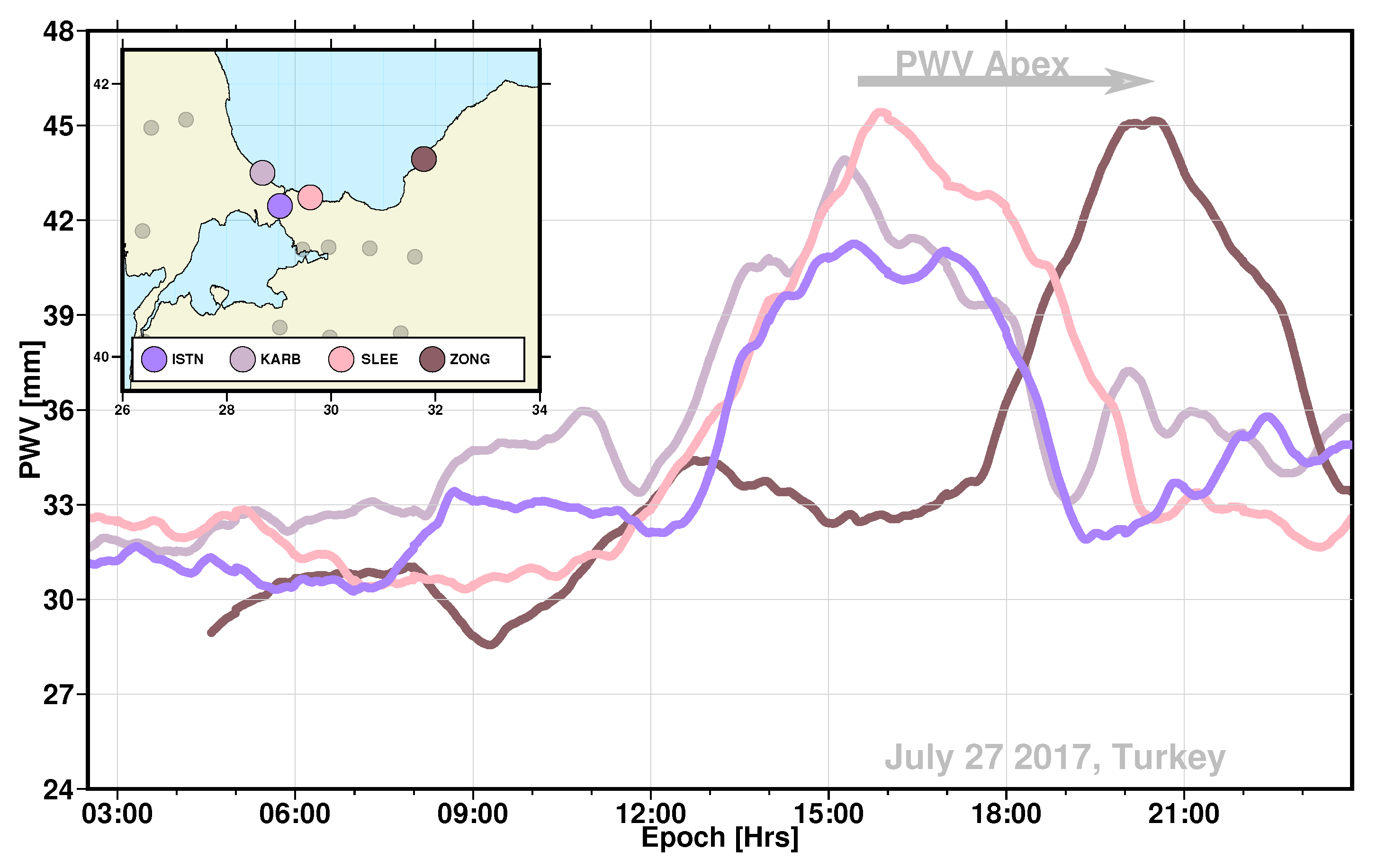
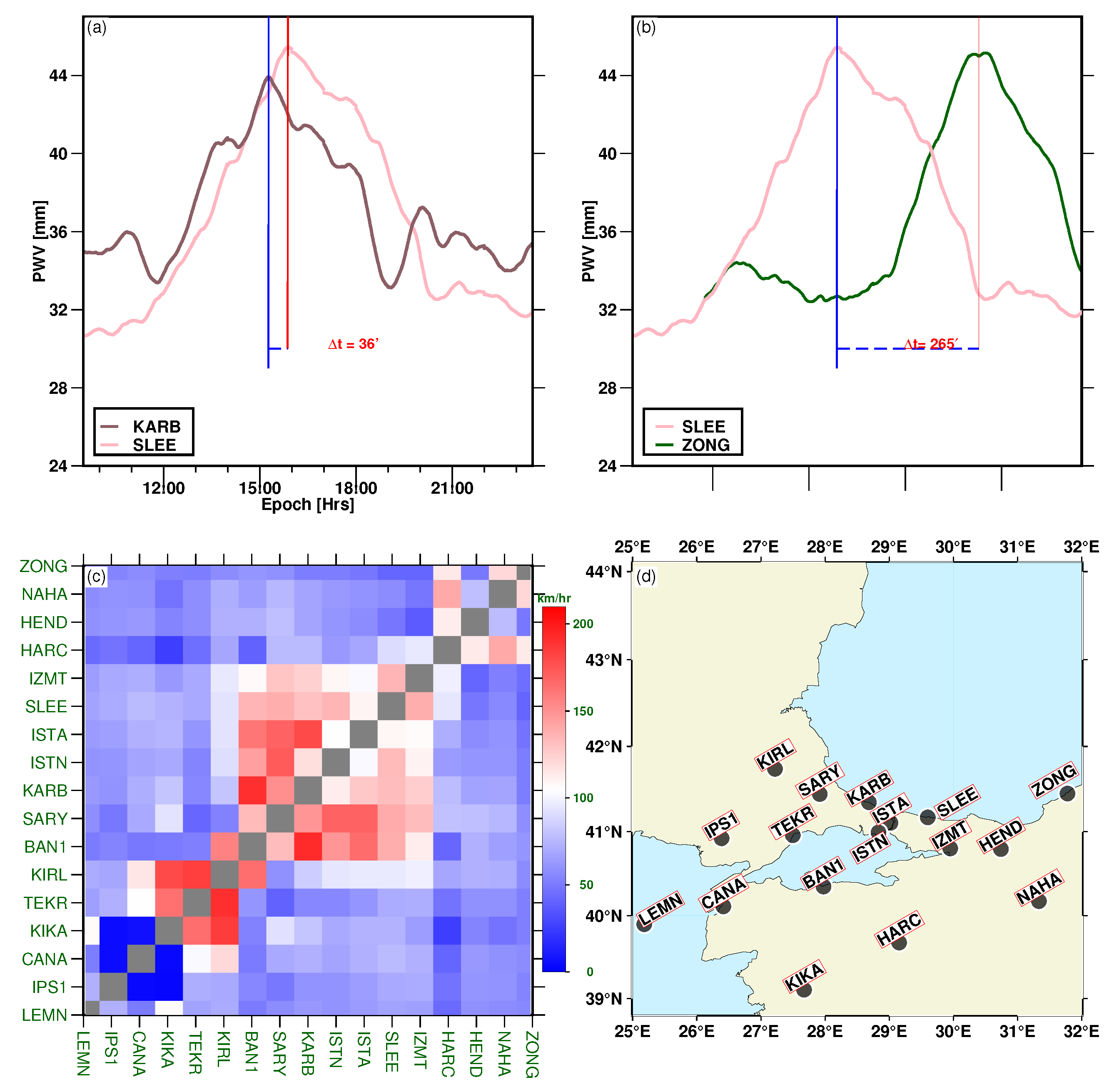
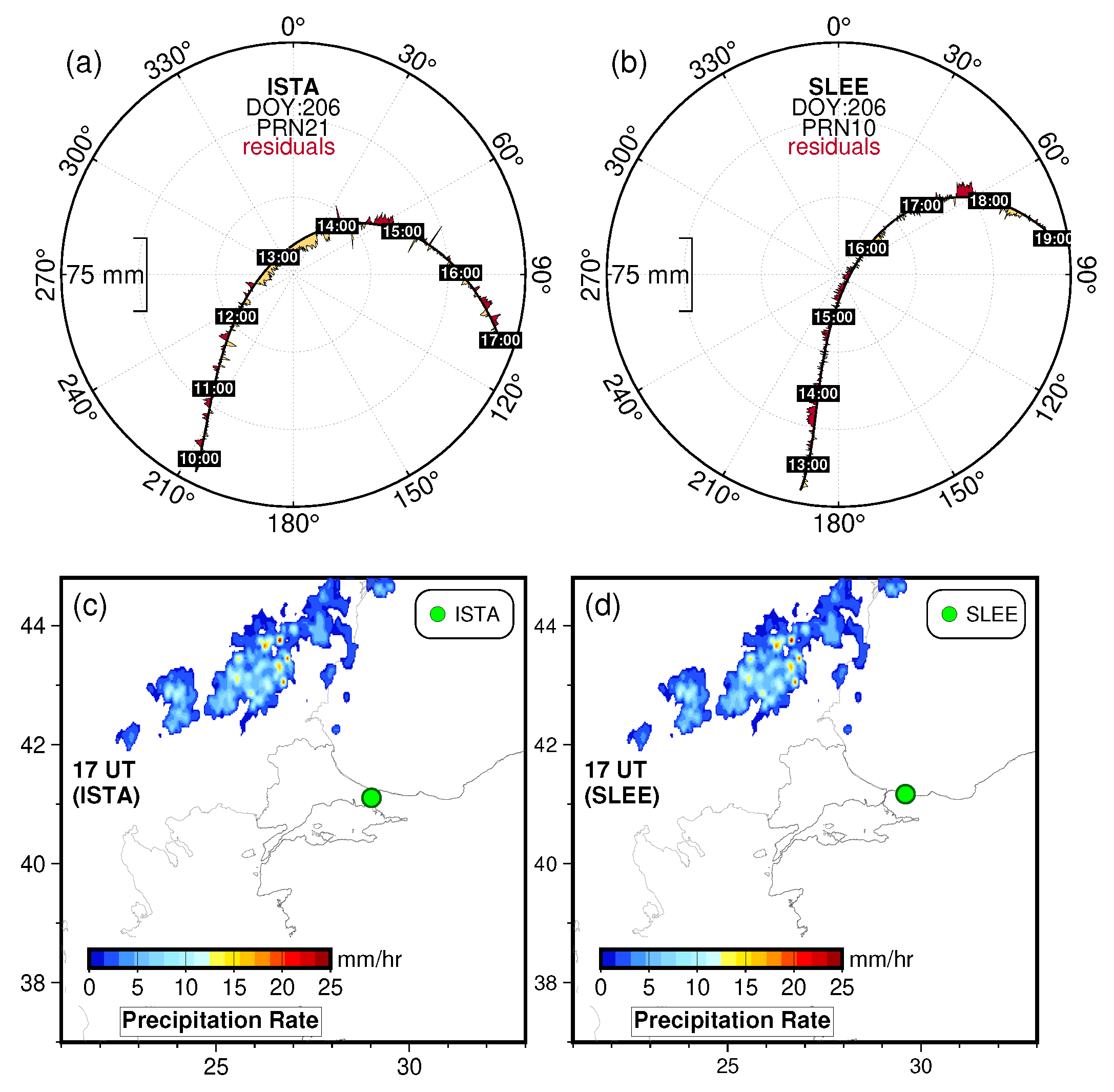
3. Severe Weather Event on 27 July 2017, in Istanbul/Turkey

On 27 July 2017, during the afternoon, a powerful supercell storm occurred in Istanbul, Turkey, that brought with it extreme weather conditions such as hailstones the size of eggs, strong winds, heavy lightning and a high amount of precipitation [56]. This rapidly growing colossal supercell, which produced large hail, led to several injuries and damaged automobiles, houses, aircraft, crops, and infrastructure in the city. To understand this extraordinary unpredicted atmospheric event, the performance of an atmospheric model, the weather research and forecast (WRF) model, was simulated using different parameterization schemes [57]. It was found that sensitivity simulations produce different rainfall distributions, and significant differences in the spatial patterns arise because of the cumulus parameterizations [56]. At the same time, microphysics schemes seem to affect the magnitude of the rainfall. According to the results, the movement of the cut-off cyclone from the Middle East and the associated transport of warm air advection increased low-level moisture convergence. Excessive wind shear values increased the thermal instability conditions and brought in thunderstorms, stormy and gale wind gusts, extreme lightning activity, large hailstones, and high hourly amounts of precipitation (38.7, 36.2, 29.8, and 27.2 mm in the Sisli, Kadikoy, Uskudar, and Fatih districts of Istanbul, respectively, between 14:00 and 15:00 UTC), within the urbanized areas of the city.

4. Slant Delay Estimates from the NWP Model—ERA5 Reanalysis Data

The microwave signals are delayed when travelling through the neutral troposphere. This delay is determined by the difference between a signal propagating at light speed in a vacuum and a signal travelling in the atmosphere (troposphere). The delay is directly proportional to the refractive index, n, which is more effectively represented as a function of the atmosphere’s refractivity, N. It is a function of the partial water vapour pressure e and temperature T [58] and can therefore be estimated using the ideal gas assumption [59].

$$N=(n-1)\times {10}^6=k_1\frac{p-e}{T}{Z}_d^{-1}+k_2\frac{e}{T}{Z}_w^{-1}+k_3\frac{e}{T}{Z}_w^{-1}$$

(1)

where p is the air pressure, and $k_1,k_2$, and $k_3$ are refractivity coefficients that can be estimated theoretically by fitting observed atmospheric observations. These constants are taken from [58], and $Z_d^{-1},Z_w^{-1}$ are the inverse compressibility factors for dry air and water vapour, respectively. Modelling the slant total delay involves the numerical integration of the air refractivity along the signal path [60]. Recently, ray-tracing approaches have become a valuable tool for determining the slant total delay [61,62]. A numerical weather prediction model represents the state of the atmosphere in three dimensions and has emerged as an essential tool for the nowcasting/forecasting of weather. The state-of-the-art global fifth generation reanalysis of ECMWF, ERA5, [41] has a much higher spatiotemporal horizontal resolution of $0.{25}^{\circ }\times 0.{25}^{\circ }$ with hourly temporal resolutions compared with its predecessors (ERA-I), from 31 vertical constant isobaric levels. The new version of ERA5 provides enhanced representations of convective systems, gravity waves, and synoptic-scale structures in the atmosphere [63]. We used the ERA5 hourly refractive model products to estimate the ZTD, slant total delay (STD) and east–west and north–south gradient estimations using a ray-tracing algorithm. From the ERA5 data, the three-dimensional refractivity field with appropriate spatial resolution and temporal resolution is derived before applying the ray-tracing algorithm. For each GPS station, we selected the four surrounding grid node values of pressure, temperature, and humidity and estimated the refractivity values using Equation (1). Horizontal interpolation is usually carried out using bilinear interpolation followed by vertical interpolation, assuming the refractivity varies linearly in the horizontal direction and exponentially in the vertical direction [62,64]. A set of ray-traced STDs for azimuth and elevation was estimated using the technique detailed in [65]. The largest error in the estimated STDs was found for the ERA5 refractivity field and an uncertainty of 10 mm close to the zenith and approximately 10 cm was found at an elevation angle of $5^{\circ }$ [66]. It is worth noting that none of our GPS tropospheric products were assimilated into the ERA5 model; this data set, therefore, provides an independent source of validation, see also [67]. The slant delay was estimated for the arc length of the ray path, $S$, utilizing the average refractive index, n, between two successive rays with an approximate formula (see, e.g., [68]):

$$\mathrm{STD}=\sum _i{S}_i(n_i-1)\times {10}^6$$

(2)

The slant delay derived from ERA5 will aid in the validation of the slant delay derived from our GPS processing method by enhancing the slant water vapour component via a reduction in stationary site-specific multipath noise through the construction of multipath stacking maps from undifferenced carrier phase residuals.

5. Construction of Multipath Stacking (MPS) Maps during Severe Weather

The post-fit one-way phase residuals include unmodelled (higher-order) atmospheric delays as well as all nonatmospheric delays such as antenna phase centre variations (PCV), station multipaths, satellite orbit errors, and unmodelled phase errors that are not taken into account during GPS analysis. For meteorological applications, the site coordinates, phase ambiguities, GPS orbits, antenna PCVs, and mean atmospheric delays can typically be properly modelled, thus the unmodelled atmospheric slant delays only dominates the post-fit one-way phase residuals and ground scattered multipath [69,70,71]. Thus, the residuals present an opportunity to extract higher-order atmospheric information as a function of azimuth and elevation around a GPS station.

Multipath stacking (MPS) maps are an effective method for filtering multipath from post-fit phase residuals. The unmodelled atmospheric delay fluctuates on a daily basis, yet the multipath repeats in real-time [72]. As a result, the daily post-fit phase residuals can be averaged across a number of days (stacking) to construct a multipath map [73]. These MPS maps can help to identify stationary multipath-affected regions as a function of elevation and azimuthal directions, see Figure 2 a potential site for multipath errors. For permanent stations, incorporating days or a few weeks of observations enables complete coverage of the sky plot. During data processing, the MPS map can be either directly subtracted from the residuals [74] or incorporated into modelled observations to correct multipath effects [75]. To project the post-fit residuals in constructing the MPS maps, the post-fit residuals are first gridded as a function of elevation and azimuth in almost congruent cells [30], forming similar grid shapes and sizes. In forming the congruent cells, the horizontal arc that subtends the azimuth remains constant with the variable azimuthal increment with increasing elevation angle. In most cases, site-specific multipath mapping employs constant resolutions in elevation and azimuth, e.g., [74,76], penalizing the number of residuals at higher elevations. For congruent grid cells, each grid cell describes an equal area in the sky, A, as shown in Equation (3)

$$A_r\left({\theta }_r^s,{\alpha }_r^s\right)=\left\{\begin{array}{c}{r}_o·d{\alpha }_i·\underset{\mathrm{arc}\mathrm{length}}{\underbrace{r_o·\cos \left({\theta }_{r,i}^s\right)·d{\alpha }_i}},{\theta }_{r,i}^s\in [0^{\circ },{90}^{\circ }]\hfill \end{array}\right.$$

(3)

where $d{\alpha }_j$ is the variable azimuthal increment in degrees and $r_o$ is the radius of the maximum horizontal circle, e.g., $d{\alpha }_o=1,r_o=180/\pi$. Even though the elevation angle, $\theta$, increases, the arc lengths show similar values because of the variable azimuth, which makes it easier to accurately measure site-specific impacts at both low and high elevation angles. Each multipath value inside each area, A, was estimated by taking the block median of the raw post-fit residuals, and the root mean square (RMS) for each grid cell. We fixed the minimum number of residuals in each bin grid to 15 following [30]. Because the grid block median value is based on the sample minimum number of residuals data and is also sensitive to outliers, rigorous statistical outlier screening tests were performed to develop a representative and reliable grid block median with the help of an iterative three-step process that consists of identification, verification, and exclusion before the stacking process was carried out. We applied the $3\sigma$ rejection rule for outlier detection, assuming normal distributions. In principle, the number of epochs required to construct the stacking map can be estimated from observations as short as a day but in general, 3–21 days provide the best results [26,77,78]. Thus, the MPS map is constructed as

$$\mathrm{M}\mathbf{P}\mathrm{S}\left({\theta }_r^s,{\alpha }_r^s\right)=\left\{\begin{array}{c}\frac{1}{N}{\displaystyle \sum _{i=1}^N}Re{s}_{r,i}^s|Re{s}_{r,i}^s\in A_r\left({\theta }_r^s,{\alpha }_r^s\right)\hfill \end{array}\right.$$

(4)

The formulation described in Equations (3) and (4), which combines all the post-fit residuals, $Re{s}_r^s$, inside area A, also termed stacking, see also [73]. To mitigate multipath impacts, we subtracted the stacked multipath map data from the raw post-fit residuals (see also [79]).

$$\overline{Res}({\theta }_r^s,{\alpha }_r^s)=Re{s}_{r,i}^s-\mathrm{MPS}({\theta }_r^s,{\alpha }_r^s)$$

(5)

Stacking was performed on the previous 21 days of raw post-fit residuals to ensure appropriate spatial coverage of cells with appropriate stacked values. The MPS map was updated by adding the most recently processed day of the post-fit residuals into the stacking map. For instance, Figure 3 depicts the one-way phase residuals as a function of satellite elevation and azimuth angles using sky-plot representations at the SARY station in Turkey on a day of the year (DOY), in 208, 2017. The lines in the map show the paths of the observed GPS satellite, with a cut-off angle of $5^{\circ }$. The grey “hole” areas represent the parts of the sky where no GPS phase residuals are available—an intrinsic design of the GPS satellite orbital inclination angle for a station located north of the equator. Figure 3a shows the raw post-fit residuals, Figure 3b shows the stacked multipath maps derived from 21 days of data using an almost congruent cells technique and lFigure 3c shows the corrected post-fit residuals that minimize the multipath footprint using Equation (5). Figure 3d illustrates alternating patterns that imply a high degree of site-specific multipaths very close to the SARY GPS station. The alternating strong scattering pattern from the GPS antenna at SARY is considered to originate from several nearby electric power lines; see Figure 2. After applying the MPS correction map, the oscillations are greatly minimized and the large residual values displayed in Figure 3a almost disappear as shown in Figure 3c. The corrected post-fit phase residuals range around ± 10 mm. Using three weeks of data significantly reduces the influence of the potential site-specific multipath errors on the residuals of the stacked values, with a reduction in RMS values across all elevation angles, most notably at low elevation angles (see Figure 3c). The site-specific multipath originated likely from several power lines in proximity to the SARY GPS station, which runs in the west to east directions (see Figure 2), is no longer visible after the multipath corrections. A similar result is also obtained for other stations, not shown here. Figure 3d shows the same representation as the MPS map in Figure 3b but plotted after surface interpolation to emphasize the footprint of a typical multipath. Additionally, the raw (in white) and corrected (in grey shade) post-fit carrier phase residual RMS value summary is presented in

Table 2. RMS of the post-fit residual before MPS map correction (in white colour) and after (shaded) with MPS map correction taken into account for different GPS stations for DOYs 201–209. See the location of the GPS stations in Figure 1.

	DOY	201	202	203	204	205	206	207	208	209
Name
AYVL		8.47	8.47	8.48	8.51	8.30	8.32	8.33	8.58	8.58
		0.65	0.66	0.66	0.67	0.65	0.66	0.65	0.66	0.67
BAN1		8.81	8.94	9.00	9.02	8.90	8.90	8.87	9.10	9.10
		0.72	0.73	0.74	0.74	0.74	0.74	0.74	0.74	0.74
COST		8.83	8.78	8.85	8.93	8.91	9.04	9.13	9.35	9.45
		0.69	0.69	0.70	0.71	0.73	0.73	0.74	0.76	0.76
HEND		13.58	13.57	13.60	13.59	13.45	13.37	13.37	13.46	13.45
		1.03	1.03	1.06	1.02	1.01	1.02	1.00	1.00	1.00
ISTN		9.59	9.56	9.80	9.86	10.05	10.05	10.02	10.23	10.23
		0.78	0.78	0.76	0.75	0.76	0.76	0.76	0.77	0.76
IZMT		11.26	11.22	11.16	10.44	10.46	10.18	10.22	10.34	10.23
		0.74	0.75	0.75	0.74	0.72	0.72	0.72	0.75	0.75
KARB		9.91	9.92	9.94	9.96	9.86	9.88	9.91	10.04	10.06
		0.77	0.78	0.78	0.77	0.78	0.78	0.79	0.82	0.82
KIRL		10.59	10.53	10.54	10.38	10.11	10.14	10.24	10.29	10.28
		0.76	0.76	0.77	0.76	0.75	0.75	0.78	0.78	0.77
SLEE		9.36	9.34	9.32	9.33	9.28	8.90	8.88	9.19	9.17
		0.66	0.66	0.66	0.66	0.64	0.63	0.64	0.67	0.66
TEKR		9.70	9.67	9.68	9.61	9.47	9.55	9.56	9.66	9.71
		0.78	0.78	0.78	0.77	0.76	0.77	0.77	0.77	0.77
ZONG		9.98	9.93	9.87	9.88	9.74	9.41	9.42	9.56	9.64
		0.78	0.78	0.76	0.77	0.75	0.72	0.73	0.77	0.76

. The applicability of the MPS map resulted in a significant reduction in the RMS of the post-fit residuals of less than 1.1 mm. Therefore, the MPS map allows the separation of site-specific multipaths and the remaining unmodelled atmospheric slant delay.

6. Retrieval of Integrated Slant Total Delay from GPS

The troposphere induces a delay in the GPS as well as in very-long-baseline interferometry (VLBI) and synthetic aperture radar (SAR) signals and is due to refractivity and scattering by tropospheric gasses and also hydrometeors [48,80]. The atmospheric refractivity is the sum of refractivity owing to dry atmospheric gases and water vapour. The relative concentration of various gases in the dry atmosphere is fairly constant and predictable and therefore is not a source of significant GNSS coordinate error [81]. Although water vapour is the most variable component of the atmosphere, it is difficult to estimate. The estimation of ZTD relies on the assumption of azimuthal symmetry [82,83], which restricts the accuracy and spatial resolution of GPS sensed water vapour, but benefits noise reduction associated with averaging on over longer time series. Alternately, one can attain a greater spatial resolution by accounting for the integrated water vapour or “slant water” delay (SWD) along each ray path between the satellite and receiver antenna. The SWD is calculated by calculating for the total slant delay along individual line of sight and then removing the dry component of the tropospheric slant total delay (STD). The carrier phase measurements, ${\Phi }_r^s$, from the GPS satellites, s, as measured by the GPS receiver, r, at a particular epoch takes the form (see, e.g., [84])

$${\Phi }_r^s={\rho }_r^s+{\mathcal{N}}_r^s\lambda +{\mathrm{STD}}_r^s-Io{n}_r^s+c({\delta }^s-{\delta }^r)+{ϵ}_i$$

(6)

where $\rho$ is the distance between the GPS satellite and receiver, $\mathcal{N}$ is carrier phase ambiguity, $\lambda$ is the wavelength, c is the speed of light in a vacuum, and $ϵ$ is the residual, which mainly comes from site specific errors. ${\delta }_r$ and ${\delta }^s$ are the receiver and satellite clock error, respectively. $\mathrm{STD}$ is the tropospheric slant delay due to the neutral atmosphere, and $Ion$ represents propagation delays due to the ionosphere. The STD cannot be computed directly from Equation (6) as the number of unknown parameters would exceed the number of observations [66,85]. The STD in Equation (6) is often represented as a function of the zenith total delay and its constituents, i.e., ZHD and ZWD (or have a first-order horizontal gradient) with particular mapping functions assuming that the atmospheric density and water vapour are uniform in the horizontal direction [86]. The primary benefit of averaging is noise reduction; however, it inevitably results in a loss of information. The availability SWD estimates may aid in reconstructing the three-dimensional tropospheric water vapour content. Determining the values of SWD and, subsequently, slant water vapour (SWV) has been the subject of extensive research and development over the past few decades. As a result, contributions to the path delay that are not captured by the model parameters in the GPS least square solutions end up in the line-of-sight post-fit residuals. They are indicative of the anisotropic component of the atmosphere [87], i.e., higher-order inhomogeneity of the atmosphere. However, the post-fit residuals are primarily influenced by unmodeled atmospheric effects, while the impact of other sources of uncertainty is minimized. In this study, we decompose the STD as the sum of isotropic and anisotropic mapping functions by including the GPS carrier phase post-fit residuals [88]. This reconstructs the separate slant delay measurement, which may contain unmodelled effects such as the 3D distribution of the state of the atmosphere as expressed in Equation (7)

$$\begin{array}{cc}\hfill \mathrm{STD}(\alpha ,\theta )=& \underset{\mathrm{isotropic}}{\underbrace{m(\theta ,a_h,b_h,c_h)·\mathrm{ZHD}+m(\theta ,a_w,b_w,c_w)·\mathrm{ZWD}}}\hfill \\ \hfill & +\underset{\mathrm{anisotropic}}{\underbrace{m_g\left(\theta \right)·[G_N·cos\left(\alpha \right)+G_E·sin\left(\alpha \right)]+\overline{Res}({\theta }_r^s,{\alpha }_r^s)}}\hfill \end{array}$$

(7)

where ZHD is the zenith hydrostatic (dry) delay and ZWD is the zenith wet delay with gradient vector $\mathbf{G}=(G_N,G_E)$, which represents the magnitude and direction of the tropospheric delay horizontal linear heterogeneity of the water vapour above each GPS station with respect to the direction of the satellites. The angles $\theta$ and $\alpha$ describe the elevation and azimuth for each observed satellite, respectively. $m_h\left(\theta \right)$ and $m_w\left(\theta \right)$ are hydrostatic and wet mapping functions with specific coefficients $a_h$; $b_h$; $c_h$ and $a_w$; $b_w$; $c_w$, respectively. The variable $m_g\left(\theta \right)$ is the horizontal gradient mapping function [89] and $\overline{Res}$ is the phase post-fit residual. The difference between the final model results of GipsyX and the ionospheric free linear combination of the $L1$ and $L2$ carrier phases and pseudorange observations, largely includes site-specific errors and other unmodelled errors during GPS data processing. It is important that the unmodelled errors should be minimized in the analysis of STD while maintaining the atmospheric anisotropy information content. To better estimate the STD, we constructed site-specific MPS maps from long-term observations by assigning the post-fit residuals as a function of the azimuth and elevation grid cells [29,74,75] and with further improvement in MPS maps by employing the almost congruent cells technique [30]. As in ZTD, STD can be separated into two components: slant hydrostatic delay (SHD) and SWD. From Equation (7), disregarding SHD, the ${\mathrm{SWD}}_r^s$ between a GPS antenna, r and satellite, s, can be written as:

$$\mathrm{SWD}{(\alpha ,\theta )}_r^s=m{\left(\theta \right)}_r^s·\mathrm{ZWD}+m_g\left(\theta \right)·[G_N·cos\left(\alpha \right)+G_E·sin\left(\alpha \right)]+\overline{Res}({\theta }_r^s,{\alpha }_r^s)$$

(8)

If we lump the ZWD and horizontal gradients together, denote the post-fit residuals now considered as a residual slant wet delay, and subsequently convert the slant wet delay to the associated slant water vapour (SWV) by conversion factor $\Pi$, Equation (8) can be written as

$$\mathrm{SWD}{(\alpha ,\theta )}_r^s=\frac{1}{\Pi }\left[{\mathrm{SWV}}_r^s+\delta {\mathrm{SWV}}_r^s\right]=m{\left(\theta \right)}_r^s\left[{\mathrm{PWV}}_r+\delta {\mathrm{PWV}}_r\right]$$

(9)

$\delta {\mathrm{SWV}}_r^s$ represents the anisotropic high-order tropospheric information derived from the post-fit residuals corrected by site-specific errors such as multipath errors and multiplied by $\Pi \left({\mathrm{T}}_m\right)$. The dimensionless quantity $\Pi$ can be estimated from the weighted average temperature profile of the atmosphere above each GPS receiver [90]. In the zenith direction, the amount of integrated water vapour is related to the length of an equivalent column of liquid water, which is customarily called precipitable water. Estimating SWV in Equation (9) brings problems compared to PWV due to noise such as unmodelled errors during GPS processing from different sources, mainly due to site-specific ground reflected multipaths. An average over a certain temporal window and from multiple satellites is needed to extract optimal information from $\delta {\mathrm{SWV}}_r^s$.

7. Results

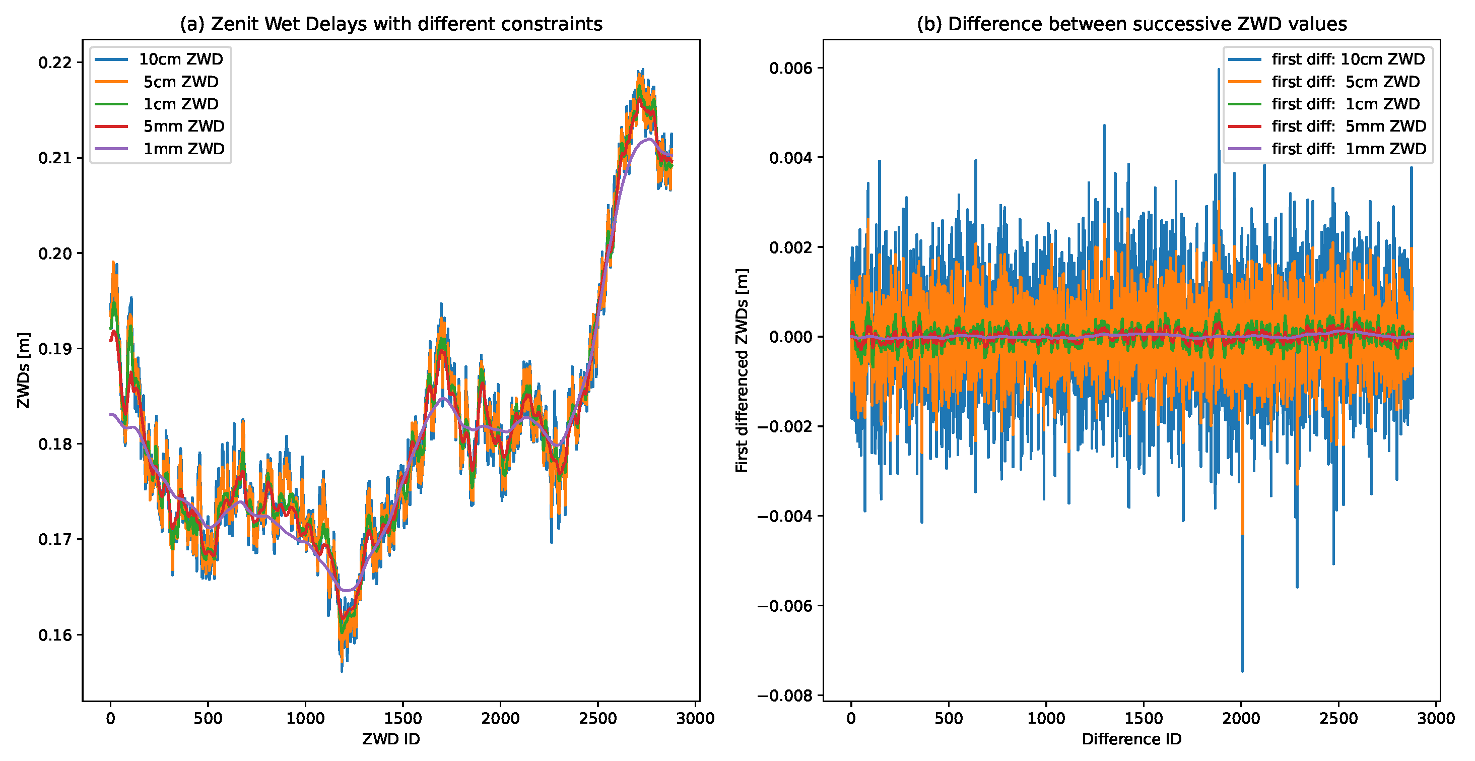
7.1. Zenith Wet Delay

This section presents the derived GPS meteorological parameters pertaining to water vapour transport and the detection of convective events. The estimated zenith wet delay from our PPP GPS processing is a proxy for the amount of water vapour in the troposphere. It can also be converted to integrated water vapour or PWV to provide more beneficial information in meteorological applications and easily compared with other in situ observations. The scaling parameter to convert from ZWD to PWV or IWV largely depends on the integrated mean temperature between the GPS station and the satellite path. The mean temperature $T_m$ is typically estimated from the surface temperature $T_s$ observed at the GPS station or from the model surface temperature following a linear relationship between them. [91] have proposed a linear relationship between $T_m$ and $T_s$ based on radiosonde data over the USA. [90] have used eight radiosonde sites using more than 4000 profiles over Turkey and computed a more appropriate model to convert the surface temperature to mean temperature.

$$T_m=0.80\times T_s+48.55$$

(10)

Figure 4 shows the precipitable water vapour every 30 s epoch in millimetres for selected stations (ISTN, KARB, SLEE, ZONG) along the coast of the Black Sea, Turkey, from our PPP solutions on DOY 208 in 2017. Similar maximum PWV values were collectively attained from the four stations as the convective storm passed the area. The PWV started to increase at a rapid rate at approximately 12 UTC at the ISTN, KARB, and SLEE stations, possibly indicating the onset of a convective storm near these stations and continued to increase until 15:15 UTC and 16 UTC for at KARB and SLEE stations, respectively. The maximum PWV content was noted in the city of Sile, Turkey, just before 16 UTC. This result correlates well with the maximum precipitation zone period based on satellite rainfall data. The rainfall estimates were obtained from the Integrated Multisatellite Retrievals for Global Precipitation Measurement (IMERG) product of the Global Precipitation Measurement (GPM) satellite program [92]. Local precipitation totals can be much more significant when measured from the ground. Soon after 16:00 UTC, the water vapour began to weaken and slowly decreased; its minimum value was found at 19:00 UTC and 20 UTC at the KARB and SLEE stations, respectively. The GPM rainfall also moved north-east towards the Black Sea, further away from Istanbul and the surrounding coastal areas. The PWV started to increase again at 17:45 sharply at the ZONG station before intense rainfall overwhelmed the area surrounding the station; it was therefore preponderant before the onset of intense precipitation. However, the PWV at ZONG station started to drop sharply and the minimum PWV was noted at approximately 21:30 UTC. One possible explanation for the drop in PWV is the transformation of water vapour into liquid water, i.e., water phase change. The wet delay is linked to the inherent dipole moment of water vapour [93]. The wet delay during GPS measurements by liquid water is proportional to the dielectric properties and, as a result, is significantly lower than the water vapour’s delay.

Landfall movement of the rainfall moved mainly from the south-west; we deduced this movement of the precipitation using the dense array of GPS stations within Turkey. By estimating the maximum cross correlation between pairs of PWV time series, it was feasible to directly estimate the time interval between the PWV crest of one station, and that of another station, or how long it takes to get from one station to another. As an example, we matched the crests of KARB and SLEE stations, as shown in Figure 5a. The maximum cross correlation between the two stations appears to match when we shifted the data from the KARB station, which is located 79 km west of the SLEE station by approximately 35 min; this implies a wind speed of up to 125 km/h. In Figure 5b, we did a similar cross-correlation between SLEE and ZONG stations, which are 186 km apart, a time shift of 265 min was needed to produce the maximum correlation with the respective PWV time series. We further expounded the cross-correlations between 17 selected stations, as shown in Figure 5d. This resulted in the heatmap plot shown in Figure 5c, which is representative of the maps of water vapour transport in the area. This indicates that the transport of the water vapour moisture field along the coast of the Black Sea revealed a maximum wind speed as the water vapour moves with much severity. In particular, the GPS-derived IWV indicated enhanced transport along Kıyıköy-Karaburun-Sile on the Black Sea coast. This transport was reduced as the water vapour field moisture moved towards Zonguldak city. Baltaci et al. [56] have shown an observed wind speed at 31.9 m/s (115 km/h) around the Kadikoy area, not far from the city of Istanbul. We also estimated a comparable wind speed in the area between the stations ISTN and IZMT, see Figure 5c,d.

7.2. Exploring Post-Fit Residuals

The post-fit residuals from the phase observations derived from our GPS processing can be used to examine each station’s data quality and environmental characteristics [54]. The post-fit residuals are a function of azimuth and elevation angles and vary depending on the multipaths scattering environment [72]. After correcting for the influence of site-specific multipath, the “cleaned” phase residual may provide more insight into the higher-order atmospheric signature during severe weather events and during the passage of convective systems. Unlike the two directional horizontal linear gradient estimates from our GPS processing, which provides the mean field, the post-fit residuals may also provide a higher-order anisotropic water vapour field from individual GPS stations along the ray path between the GPS station and a satellite (see also, [94]). Figure 6 shows the changes in the post-fit residuals for two satellites, PRN10 and PRN21, plotted as a function of the azimuth and elevation angles for DOY 206, a dry day. Figure 7 shows the severe weather conditions (DOY 208) at SLEE station. The post-fit residuals in wetter areas (positive values, shown in red) and drier areas (negative values, shown in yellow) reflect an excursion normal to the satellite tracks. Regarding the satellite tracks for both satellites on DOY 208, the post-fit residual size dramatically increased at approximately 16:00 UTC, suggesting weather condition and anisotropic atmospheric variations. To confirm the sources of these elevated post-fit residuals, we plotted the global gridded precipitation from the Integrated Multi-SatellitE Retrievals for GPM (IMERG), a product of the Global Precipitation Measurement (GPM) satellite mission [92]. Indeed, the lower panels in Figure 7 show a significant precipitation rate at approximately 16:00 UTC, which coincides with significant variations in the post-fit residuals at both the ISTA and SLEE stations. This indirectly shows that this atmospheric phenomenon is poorly modelled using GPS processing; instead, this signal is relegated as part of the error budget in the form of post-fit residuals. As for DOY 206, a dry day, the phase residuals do not reflect any enhancements; on the other hand, the post-fit residuals on DOY 208, a wet day, reflect changes in the weather conditions in the area. The RMS scatter significantly increased from 4.5 mm to 11.4 mm for the PRN21 satellite on DOYs 206 and 208, respectively. The RMS scatter for the PRN10 satellite changed from 4.1 mm to 14.1 mm on DOYs 206 and 208, respectively. These results suggest that the post-fit residuals contain additional anisotropic atmospheric moisture fields that are not present in the isotropic background precipitable water vapour typically estimated from the zenith wet delay, albeit site-specific multipaths could potentially be present. If uncorrected, the multipath maps could be mismodelled onto the phase residuals. One caveat is that the post-fit carrier phase residuals show some dependencies in the amount of constraint applied to the ZWD and horizontal linear gradients. We performed five runs of constraint variations of ZWD and horizontal linear gradients by a random walk process with the following noise intensities: 1 mm /$\surd h$ and 0.1 mm /$\surd h$; 5 mm/$\surd h$ and 0.5 mm /$\surd h$; 10 mm/$\surd h$ and 0.1 mm/$\surd h$; 50 mm/$\surd h$ and 5 mm/$\surd h$; and finally, 100 m/$\surd h$ and 10 mm/$\surd h$. The modulus of the post-fit variations from the five runs is shown in Figure 8 and varies according to the constraint set to ZWD and horizontal linear gradients during our GPS processing. The post-fit residual variations are more apparent, particularly when the convective storm strikes the area as captured by the SLEE station in Figure 8a and the ISTN station in Figure 8b. When the ZWD and horizontal gradients are constrained tightly, i.e., at noise intensities of 1 mm /$\surd h$ and 0.1 mm /$\surd h$, respectively, the post-fit residuals become unusually higher during severe weather events, shown in solid red colour. In contrast, the post-fit residuals are of a smaller magnitude when the constraint is loose/relaxed, as shown in solid pink colour in Figure 8a,b. For the two extreme constraints, up to 60 mm differences in post-fit residuals could be observed as shown in Figure 8a for the station SLEE. However, well before the storm strikes the area, the post-fit residuals show negligible dependencies on the amount of constraint set to the post-fit residuals. On the other hand, the ZWD estimate shows more variability when the constraint is loose and less variability when the constraint is tight, as shown in Figure 9.

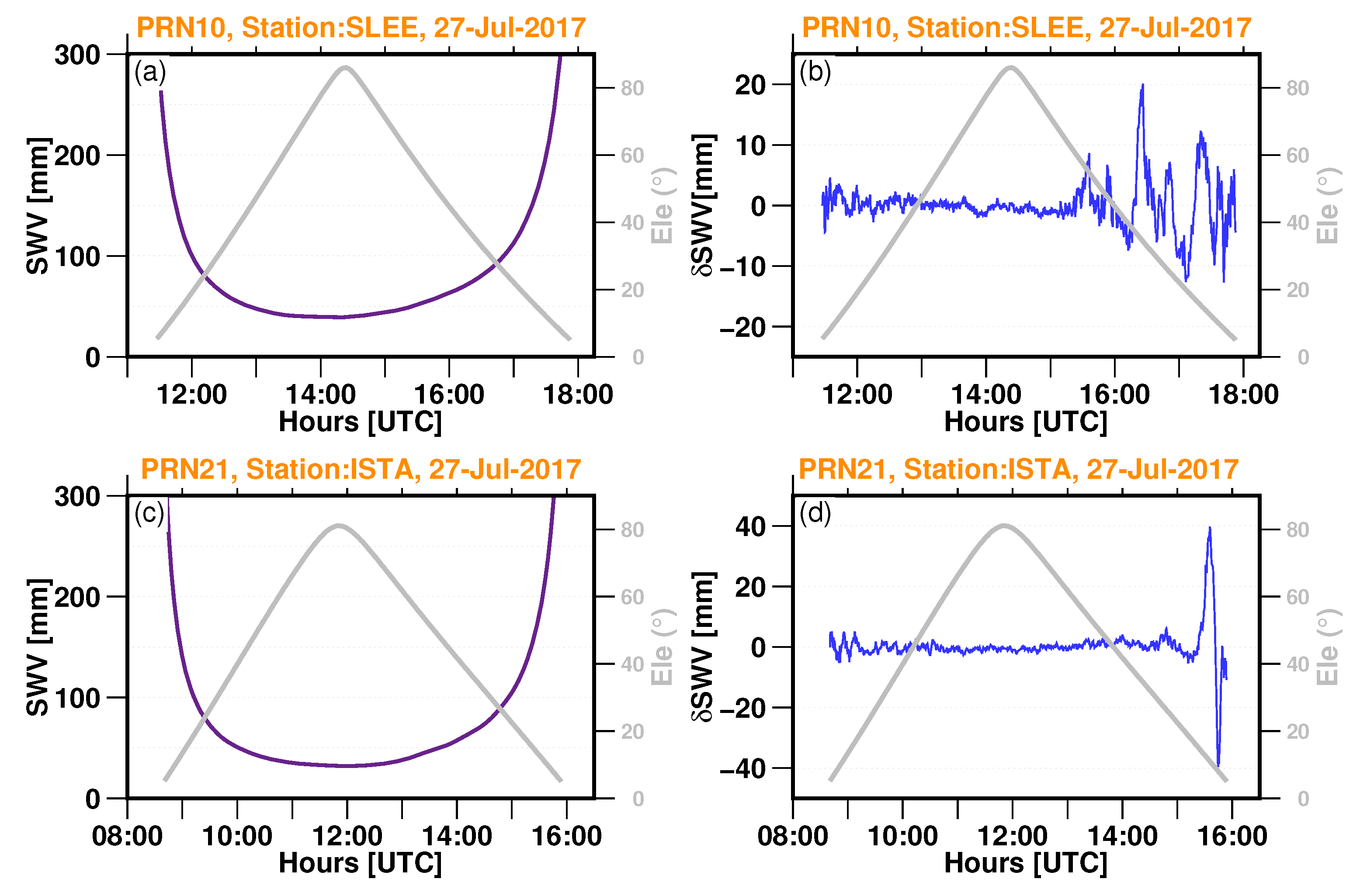
7.3. Isotropic and Anisotropic Slant Perceptible Water Vapour

In this section, we show the influence of moisture and small-scale variation observed in the anisotropic component of the slant precipitable water vapour ($\delta \mathrm{SWV}$) associated with severe weather convective storms. In general, the isotropic component is the dominant factor the SWD measurements (with the implicit assumption that the dry component is already subtracted from the total slant delay), and its temporal variation closely mirrors the changes in PWV. The anisotropic component, $\delta {\mathrm{SWV}}_r^s$, can be estimated by first modelling and consequently removing the delay that contributes to geometrical delays (troposphere, ionosphere), and clock delays, using the second term in Equation (9). The anisotropic component of the SWD, is therefore, constructed from phase observations minus the model, which invariably may contain unmodelled useful information for weather models. Figure 10a,c show the isotropic component of the slant precipitable water vapour, SWV, along the direction of individual satellites during severe weather events. Figure 10b,d show the anisotropic component the precipitable slant water vapour, and its magnitude attains a maximum of 20 mm the SLEE station and as large as 40 mm at the ISTA station. At the SLEE station, the anisotropic variation is as large as 12 mm, scaled to the zenith, of the equivalent isotropic precipitable water vapour, and at the ISTA station, this variation is as large as 7 mm in equivalent perceptible water vapour. In these severe weather conditions, the $\delta \mathrm{SWV}$ is reconstructed from the unmodelled line-of-sight post-fit residuals with magnitudes that are as much as 20% of the isotropic component, i.e., the SWV. The elevation angle in Figure 10 is shown in grey, indicating the longer paths each individual satellite takes through the planetary boundary layer.

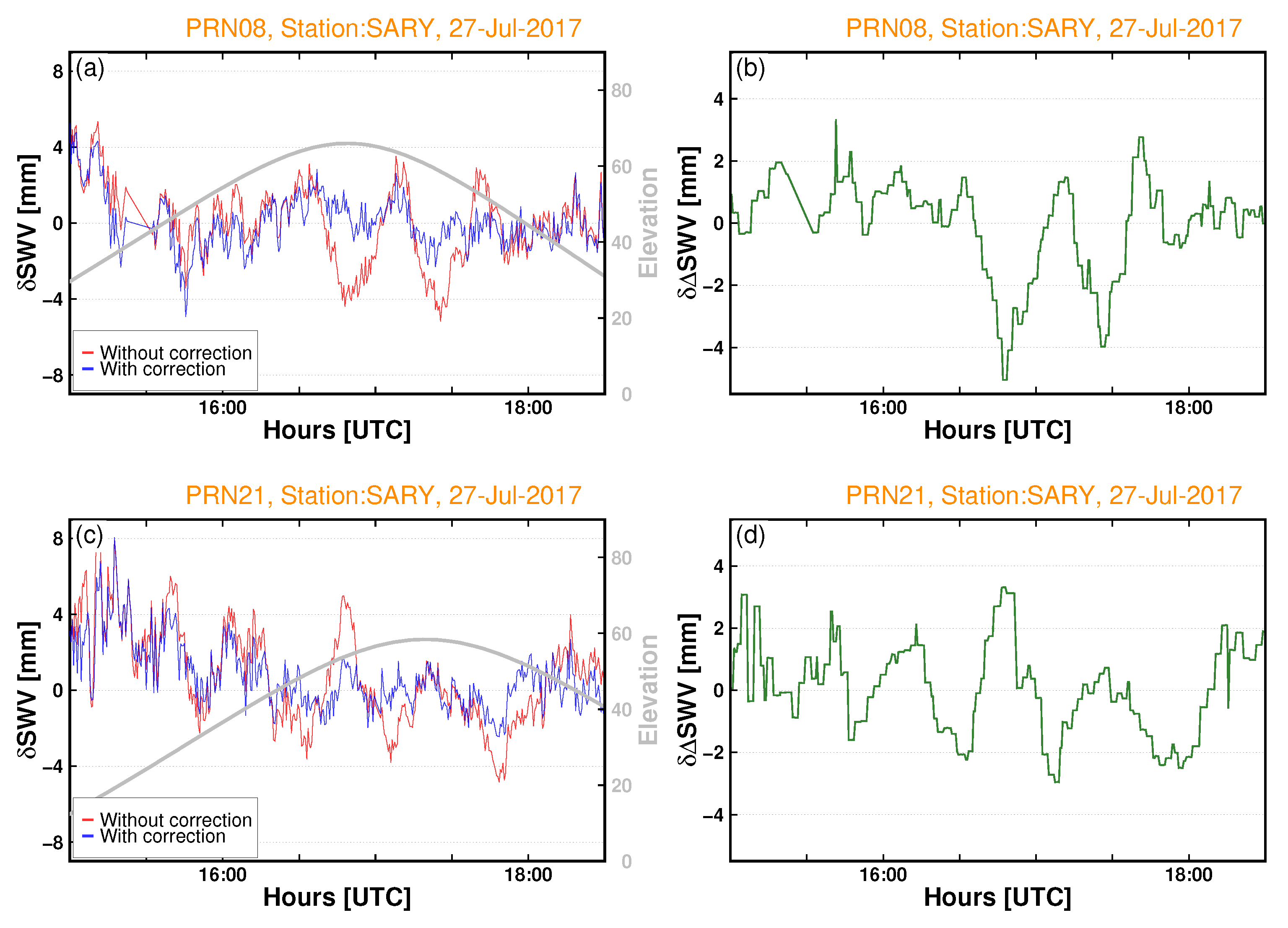
7.4. Influence of the MPS on the Anisotropic Perceptible Slant Water Vapour

Following the construction of the MPS maps in Section 5, we applied the multipath signature to reduce its influence before converting the post-fit residuals to the anisotropic precipitable slant water vapour component. As stated in Section 5, the post-fit residuals contain primarily multipaths in addition to higher-order atmospheric signals. To reduce these errors, the post-fit residuals were averaged for 21 days to produce the MPS maps as shown in Figure 3. The time series in Figure 11 shows the anisotropic precipitable slant water vapour observations in the direction of an individual satellite with and without applying site-specific multipath correction modelling. Figure 11a,b contain the anisotropic, $\delta \mathrm{SWV}$, without multipath corrections in red and with multipath corrections in blue. Figure 11c again shows the anisotropic slant precipitable water vapour for satellite PRN21 before (in red) and after (in blue) the MPS map corrections are enforced. It is again evident that the multipath effect at the SARY station shows a pronounced effect even at such a high satellite elevation angle and shows all the multipath characteristics. It is therefore necessary to apply multipath corrections. As a result, this effect is reduced; see the blue solid line in Figure 11c. Figure 11b,d show the difference between the corrected and uncorrected anisotropic slant precipitable water vapour, with magnitudes ranging between $-5$ mm to 3 mm. At the SARY station, 5 mm variations in SPWV can induce as much as 4.3 mm in equivalent PWV at the ${60}^{\circ }$ elevation angle. The satellite elevation angles for PRN08 and PRN12 as seen from the SARY station are plotted in grey.

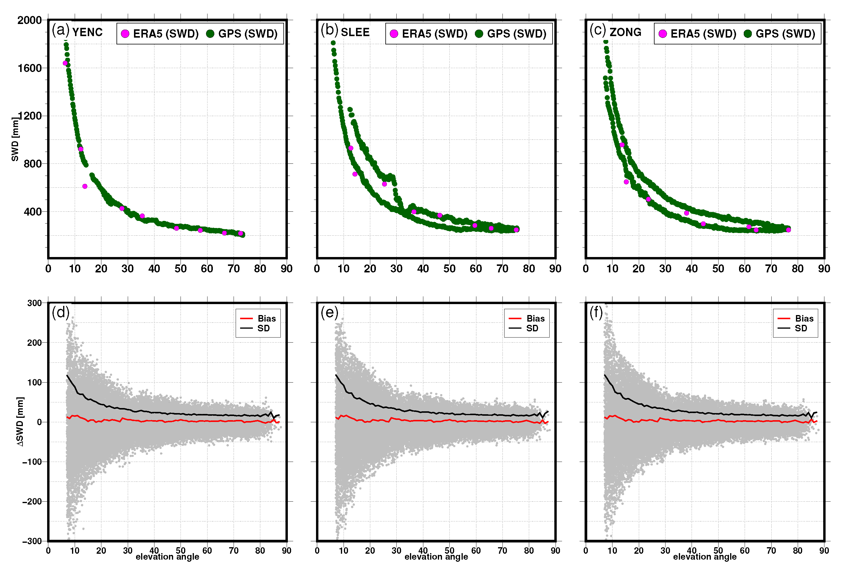
8. Validation Comparisons of GPS-Based Slant Water Vapour with ERA5

Our PPP processing does not directly determine the SWD. However, we reconstructed the slant wet delay from the zenith wet delay projected to the line-of-sight and incorporated the linear gradients and the anisotropic residuals from the post-fit residuals. Typically, a collocated water vapour microwave radiometer (WVR) measurement is used to compare the GPS-derived slant water delay [25,26]. Because no GPS station in our study area is equipped with a WVR instrument, we instead focused our comparisons with that of the ERA5 model derived slant total delay using ray-tracing techniques [65,66]. ERA5 has limited temporal and spatial resolution and offers no small-scale water vapour fluctuations; thus, the comparison with the GPS slant delay has some caveats. Because the slant wet delay in Figure 12 exhibits a considerable elevation angle dependency (the smaller the elevation angles are, the greater the GPS signal travel time delays generated by the atmosphere), it is, therefore, advantageous to plot the discrepancies between GPS and ERA5 SWDs as a function of elevation angle. At a higher elevation angle, the agreement is much better, as depicted for the YENC station in Figure 12a, for the SLEE station in Figure 12b, for the ZONG station in Figure 12c. The green circles represent the GPS-derived SWD at 30 s epoch resolution, and the magenta circles represent the ERA5 model-derived SWD at an hourly resolution. As shown in Figure 12b for the SLEE station, the ERA5 model is incapable of resolving the atmospheric variability structure of the SWD between 15 and 20-degree elevation angles, for DOY 208, coinciding with the severe weather event. Figure 12d–f shows, more conveniently, the differences between ERA and GPS-derived SWD ($\Delta \mathrm{SWD}$) for the case where the post-fit residuals along with the MPS correction maps are incorporated, only the residuals are included in the SWD and finally for the case where neither the post-fit residuals nor the MPS correction maps are incorporated, respectively. The $\Delta \mathrm{SWD}$ is depicted in solid grey circle represents an individual SWD difference with outlying differences initially identified using the widely known 3-sigma rule and consequently removed. Finally, the derived average bias (red line) and standard deviations (SDs) (in black line) of the differences for all the 55 GPS stations for DOY 206, 2017 until DOY 210, 2017 is depicted in Figure 12d–f. The SDs and the bias were computed for the elevation angles $7^{\circ }$–${90}^{\circ }$ with a step size of $1^{\circ }$. In particular, the standard deviation shows elevation angle dependencies, whereas the bias shows little to no elevation angle dependencies. The bias between GPS and ERA5 SWD is about 2.91 mm and the SD at 40.96 mm for the case neither the post-fit residuals nor the MPS correction maps are incorporated in the comparisons. The bias between GPS and ERA5 SWD is about 3.00 mm, and the SD becomes 42.96 mm including the raw post-fit residuals only. For the case with post-fit residuals and MPS corrections are applied in the GPS-derived SWD, the bias difference is 2.99 mm and the standard deviation becomes 42.50 mm.

9. Discussion

In this study, we estimated the isotropic component of the slant wet delay (SWD) and the unmodelled line-of-sight related to the anisotropic component of the SWD. For studies concerning severe atmospheric conditions and other convective initiation processes, a numerical weather prediction model will benefit from a more spatially detailed reconstruction of isotropic and anisotropic components of the SWD from the line-of-sight observations. In order to determined whether the observed high anisotropic values are the signature of atmospheric properties, we compared our PWV with the rainfall data from GPM and a good match was noted. We showed that the $\delta \mathrm{SWV}$ constructed from our GPS post-fit residuals significantly increased during severe atmospheric conditions; a similar result was also found in [10]. An elevated value of $\delta \mathrm{SWV}$ was not found for the same station during a drier day, and thus suggesting that the $\delta \mathrm{SWV}$ enhancement during storm events was due to rain scattering. During the severe weather event in Turkey, we found the anisotropic component to be as large as 20% of the isotropic component of the precipitable water vapour; a similar result was also achieved in [82]. Thus, the reconstructing of $\delta \mathrm{SWV}$ from post-fit residuals from GPS processing could be useful for rain characterization for tomography studies [86] and data assimilation in NWP models [10]. However, the direct construction of the $\delta \mathrm{SWV}$ from post-fit residuals is not possible. The post-fit residuals include several noise sources, mainly due to site-specific multipaths, unmodelled satellite orbits, clocks, antenna phase centre variations, and errors in mapping functions. Thus, a filtering technique is necessary to reduce these sources of noise. In this study, a multipath stacking map was devised using 21 days of post-fit residuals, and a correction was applied to reduce the multipath noise, which has been shown to severely affect the SARY station in Turkey, likely due to the nearby electric power lines. Our multipath stacking filter reduced the RMS values from 13 mm to 1 mm, a significant improvement using an almost congruent cell technique [30], which improves the number of post-fit residuals represented across all elevation angles. The study further elucidated that the multipath effect for severely affected areas due to many scattering environments around the GPS station adversely affects the estimated post-fit residuals. For a station such as SARY, where the scattering environment affected the GPS signal at even higher elevations, as depicted in Figure 4, the effect on the anisotropic component of the slant wet delay reached up to 5 mm, that is an equivalent precipitable water vapour signal of 4.3 mm when scaled to the zenith direction. For global NWP models, the accuracy threshold for PWV (IWV) is 5 mm, as shown in the EUMETNET EIG GNSS water vapour program [95] or based on the World Meteorological Organisation (https://space.oscar.wmo.int/variables/view/integrated_water_vapour_iwv accessed on 15 November 2022). Thus, the induced error of 4.3 mm due to the uncorrected multipath to the anisotropic contributions almost reached the threshold of what is required for numerical weather prediction but is certainly much larger than the goal, which is an accuracy threshold of with a goal of 1 mm [95]. Given the variability of the atmospheric heterogeneity during severe weather events, in this respect, we used a 30 s sampling interval for tropospheric delay estimation using the GipsyX v1.7 software, but also looked at the impact of the processing parameters in particular random walk parameters of the noise in the zenith wet delay and horizontal gradients. Depending on the choice of the random walk constraint, the post-fit residuals varied significantly. If the constraint was chosen loosely, the post-fit residuals decreased, as most of the variability goes to the estimated ZWD and gradients, and when the constraint became tighter, the post-fit residuals become significantly larger while the variability in the ZWD and horizontal gradients estimate decreased. Nevertheless, this is not the case during a dry day, with almost negligible dependency on the constraints applied to the random walk process. We showed the findings of comparing the ERA5 NWM ray tracing results with the GPS-derived slant wet delay. The biases between the GPS-derived and ERA5 show almost negligible differences whether or not we took into account the post-fit residuals, cleaned post-fit residuals by including MPS correction maps and without the post-fit residuals. The impact of incorporating the cleaned post-fit residuals only show a marginal improvement in the bias and standard deviations, with a somewhat worse bias and standard deviation relative to the raw SWD estimate from GPS solution.

10. Conclusions

The results of the case studies suggest that slant tropospheric delay based on post-fit residuals represents the inhomogeneous distribution of water vapour along the ray path between the satellite and receiving antennas, which is not modelled by the mapping function and a linear tropospheric gradient model. During the drier days, the post-fit residual offers little to no information regarding the atmosphere is inhomogeneity compared to the wetter days, as most of the variations are captured by ZTD and/or horizontal gradients. On the other hand, during the passage of the severe weather system that caused a catastrophic flood in Istanbul, Turkey, in July 2017, the one-way post-fit residuals at multiple GPS stations exhibited significant increases in their values. We thus conclude that the slant tropospheric delay contains physically meaningful information for monitoring water vapour activity during periods of convective weather conditions. The technique of sensing precipitable slant water vapour has the potential to provide finer atmosphere variability and can be further input to numerical weather models for nowcasting and forecasting. In the event of severe weather, the reconstructed anisotropic atmospheric structure from post-fit residuals provides a fine structure of the atmosphere; nevertheless, it is highly impacted by site-specific multipaths at low elevation angles and, even surprisingly, at higher elevation angles. We found that the anisotropic component of the precipitable water vapour during the severe weather event in Turkey could reach as large as $20\%$ of the isotropic component. With the numerical weather prediction requirements of the accuracy of PWV, i.e., a threshold of 5 mm, this study shows that the multipath errors need to be reduced to provide sufficiently accurate PWV estimates. Our new multipath stacking maps include any intrinsic antenna phase centre variations and any stationary site-specific noise resulting in the surrounding scattering environment that occurs at a regular spatial interval as a function of elevation and azimuth. Thus, the MPS maps perform well; in doing so, the stacking map can potentially be used to improve the accuracy of other geodetic parameter estimates as well and be useful to provide further information in GPS water tomography modelling. Furthermore, the constraints as a random walk process significantly impact the post-fit residuals during the passage of convective weather event. The choice of the constraint determines the magnitude of the anisotropic information resulting from our GPS processing to reflect the rapid variability of the atmosphere. In GPS processing, the inferred zenith wet delay and horizontal gradient temporal variation as a random walk stochastic process are assumed but are not adequately represented during high-impact weather events. Our sensitivity study of the constraints shows that the choice of stochastic process noise results in significant differences in the magnitude of post-fit residuals. An optimal choice of the constraint can be inferred from using nearby collocated microwave radiometer measurements. The results of our GPS-based slant wet delay are compared with those of the ERA5 reanalysis estimated slant wet delay. The differences in SWD between GPS and ERA5 show a dependency on the elevation angle, with higher differences manifested at lower elevations indicating longer path traversed by individual satellites take through the planetary boundary but much lower values close to the zenith direction. On the other hand, the fractional SWD showed no dependencies to elevation angle. However, the model slant wet delay from the ERA5 model is far from resolving the atmospheric variability during severe weather events.

References

1. Liang, X.Z. Extreme rainfall slows the global economy. Nature 2022, 601, 193–194. [Google Scholar] [CrossRef] [PubMed]
2. IPCC. Fifth Assessment Report (AR5): Climate Change 2013/2014. Climate Change 2014: Impacts, Adaptation, and Vulnerability; Cambridge University Press: New York, NY, USA, 2014; OCLC: 956694305. [Google Scholar]
3. Trenberth, K.E.; Smith, L. The Mass of the Atmosphere: A Constraint on Global Analyses. J. Clim. 2005, 18, 864–875. [Google Scholar] [CrossRef]
4. Houghton, J.T.; Callander, B.A.; Varney, S.K.; Intergovernmental Panel on Climate Change (Eds.) Climate Change 1992: The Supplementary Report to the IPCC Scientific Assessment; Cambridge University Press: Cambridge, UK; New York, NY, USA, 1992. [Google Scholar]
5. Ahrens, C.D.; Samson, P.J. Extreme Weather and Climate, 1st ed.; Brooks/Cole, Cengage Learning: Belmont, CA, USA, 2010. [Google Scholar]
6. Jones, J.; Guerova, G.; Douša, J.; Dick, G.; Haan, S.d.; Pottiaux, E.; COST Association (Eds.) Advanced GNSS Tropospheric Products for Monitoring Severe Weather Events and Climate: COST Action ES1206 Final Action Dissemination Report; Springer: Cham, Switzerland, 2020. [Google Scholar]
7. Baltaci, H. Meteorological characteristics of dust storm events in Turkey. Aeolian Res. 2021, 50, 100673. [Google Scholar] [CrossRef]
8. Brenot, H.; Ducrocq, V.; Walpersdorf, A.; Champollion, C.; Caumont, O. GPS zenith delay sensitivity evaluated from high-resolution numerical weather prediction simulations of the 8–9 September 2002 flash flood over southeastern France. J. Geophys. Res. 2006, 111, D15105. [Google Scholar] [CrossRef] [Green Version]
9. Moore, A.W.; Small, I.J.; Gutman, S.I.; Bock, Y.; Dumas, J.L.; Fang, P.; Haase, J.S.; Jackson, M.E.; Laber, J.L. National Weather Service Forecasters Use GPS Precipitable Water Vapor for Enhanced Situational Awareness during the Southern California Summer Monsoon. Bull. Am. Meteorol. Soc. 2015, 96, 1867–1877. [Google Scholar] [CrossRef]
10. Champollion, C.; Masson, F.; Bouin, M.N.; Walpersdorf, A.; Doerflinger, E.; Bock, O.; Van Baelen, J. GPS water vapour tomography: Preliminary results from the ESCOMPTE field experiment. Atmos. Res. 2005, 74, 253–274. [Google Scholar] [CrossRef] [Green Version]
11. Singh, R.; Ojha, S.P.; Puviarasan, N.; Singh, V. Impact of GNSS Signal Delay Assimilation on Short Range Weather Forecasts Over the Indian Region. J. Geophys. Res. Atmos. 2019, 124, 9855–9873. [Google Scholar] [CrossRef]
12. Iwabuchi, T.; Rocken, C.; Wada, A.; Kanzak, M. True Real-time Slant Tropospheric Delay Monitoring System with Site Dependent Multipath Filtering. In Proceedings of the 24th International Technical Meeting of the Satellite Division of The Institute of Navigation (ION) GNSS 2011), Portland, OR, USA, 20–23 September 2011; pp. 579–587. [Google Scholar]
13. Ducrocq, V.; Ricard, D.; Lafore, J.P.; Orain, F. Storm-Scale Numerical Rainfall Prediction for Five Precipitating Events over France: On the Importance of the Initial Humidity Field. Weather. Forecast. 2002, 17, 1236–1256. [Google Scholar] [CrossRef]
14. Benevides, P.; Catalao, J.; Miranda, P.M.A. On the inclusion of GPS precipitable water vapour in the nowcasting of rainfall. Nat. Hazards Earth Syst. Sci. 2015, 15, 2605–2616. [Google Scholar] [CrossRef] [Green Version]
15. Benevides, P.; Catalao, J.; Nico, G. Neural Network Approach to Forecast Hourly Intense Rainfall Using GNSS Precipitable Water Vapor and Meteorological Sensors. Remote Sens. 2019, 11, 966. [Google Scholar] [CrossRef]
16. Hocke, K.; Navas-Guzman, F.; Moreira, L.; Bernet, L.; Mätzler, C. Diurnal Cycle in Atmospheric Water over Switzerland. Remote Sens. 2017, 9, 909. [Google Scholar] [CrossRef] [Green Version]
17. Shoji, Y.; Kunii, M.; Saito, K. Assimilation of Nationwide and Global GPS PWV Data for a Heavy Rain Event on 28 July 2008 in Hokuriku and Kinki, Japan. SOLA 2009, 5, 45–48. [Google Scholar] [CrossRef] [Green Version]
18. Ejigu, Y.G.; Teferle, F.N.; Klos, A.; Bogusz, J.; Hunegnaw, A. Tracking Hurricanes Using GPS Atmospheric Precipitable Water Vapor Field; Springer: Berlin/Heidelberg, Germany, 2020. [Google Scholar]
19. Ejigu, Y.G.; Teferle, F.N.; Klos, A.; Bogusz, J.; Hunegnaw, A. Monitoring and prediction of hurricane tracks using GPS tropospheric products. GPS Solut. 2021, 25, 76. [Google Scholar] [CrossRef]
20. Järvinen, H.; Eresmaa, R.; Vedel, H.; Salonen, K.; Niemelä, S.; de Vries, J. A variational data assimilation system for ground-based GPS slant delays. Q. J. R. Meteorol. Soc. 2007, 133, 969–980. [Google Scholar] [CrossRef]
21. Kawabata, T.; Shoji, Y.; Seko, H.; Saito, K. A Numerical Study on a Mesoscale Convective System over a Subtropical Island with 4D-Var Assimilation of GPS Slant Total Delays. J. Meteorol. Soc. Jpn. Ser. II 2013, 91, 705–721. [Google Scholar] [CrossRef] [Green Version]
22. Ware, R.; Alber, C.; Rocken, C.; Solheim, F. Sensing integrated water vapor along GPS ray paths. Geophys. Res. Lett. 1997, 24, 417–420. [Google Scholar] [CrossRef] [Green Version]
23. Masoumi, S.; McClusky, S.; Koulali, A.; Tregoning, P. A directional model of tropospheric horizontal gradients in Global Positioning System and its application for particular weather scenarios: Directional Tropospheric Gradients. J. Geophys. Res. Atmos. 2017, 122, 4401–4425. [Google Scholar] [CrossRef]
24. Eresmaa, R.; Järvinen, H.; Niemelä, S.; Salonen, K. Asymmetricity of ground-based GPS slant delay data. Atmos. Chem. Phys. 2007, 7, 3143–3151. [Google Scholar] [CrossRef] [Green Version]
25. Braun, J.; Rocken, C.; Ware, R. Validation of line-of-sight water vapor measurements with GPS. Radio Sci. 2001, 36, 459–472. [Google Scholar] [CrossRef] [Green Version]
26. Braun, J.; Rocken, C.; Liljegren, J. Comparisons of Line-of-Sight Water Vapor Observations Using the Global Positioning System and a Pointing Microwave Radiometer. J. Atmos. Ocean. Technol. 2003, 20, 606–612. [Google Scholar] [CrossRef]
27. Shoji, Y.N.N.; Iwabuchi, T.; Aonashi, K.; Seko, H.; Mishima, K.; Itagaki, A.; Ichikawa, R.; Ohtani, R. Tsukuba GPS Dense Net Campaign Observation: Improvement in GPS Analysis of Slant Path Delay by Stacking One-way Postfit Phase Residuals. J. Meteorol. Soc. Jpn. 2004, 82, 301–314. [Google Scholar] [CrossRef] [Green Version]
28. Li, X.; Zus, F.; Lu, C.; Ning, T.; Dick, G.; Ge, M.; Wickert, J.; Schuh, H. Retrieving high-resolution tropospheric gradients from multiconstellation GNSS observations. Geophys. Res. Lett. 2015, 42, 4173–4181. [Google Scholar] [CrossRef] [Green Version]
29. Sidorov, D.; Teferle, F. Impact of Antenna Phase Centre Calibrations on Position Time Series. Preliminary Results; Springer: Berlin/Heidelberg, Germany, 2016; Volume 143, pp. 117–123. [Google Scholar]
30. Fuhrmann, T.; Luo, X.; Knöpfler, A.; Mayer, M. Generating statistically robust multipath stacking maps using congruent cells. GPS Solut. 2015, 19, 83–92. [Google Scholar] [CrossRef]
31. Zumberge, J.F.; Heflin, M.B.; Jefferson, D.C.; Watkins, M.M.; Webb, F.H. Precise point positioning for the efficient and robust analysis of GPS data from large networks. J. Geophys. Res. Solid Earth 1997, 102, 5005–5017. [Google Scholar] [CrossRef] [Green Version]
32. Nilsson, T.; Elgered, G. Long-term trends in the atmospheric water vapor content estimated from ground-based GPS data. J. Geophys. Res. 2008, 113, D19101. [Google Scholar] [CrossRef] [Green Version]
33. Bertiger, W.; Bar-Sever, Y.; Dorsey, A.; Haines, B.; Harvey, N.; Hemberger, D.; Heflin, M.; Lu, W.; Miller, M.; Moore, A.W.; et al. GipsyX/RTGx, a new tool set for space geodetic operations and research. Adv. Space Res. 2020, 66, 469–489. [Google Scholar] [CrossRef]
34. Miyazaki, S.; Iwabuchi, T.; Heki, K.; Naito, I. An impact of estimating tropospheric delay gradients on precise positioning in the summer using the Japanese nationwide GPS array. J. Geophys. Res. Solid Earth 2003, 108. [Google Scholar] [CrossRef]
35. Gelb, A.; Analytic Sciences Corporation (Eds.) Applied Optimal Estimation, 14th ed.; MIT Press: Cambridge, MA, USA, 1996. [Google Scholar]
36. Herring, T.A.; Davis, J.L.; Shapiro, I.I. Geodesy by radio interferometry: The application of Kalman Filtering to the analysis of very long baseline interferometry data. J. Geophys. Res. 1990, 95, 12561. [Google Scholar] [CrossRef]
37. Hadas, T.; Teferle, F.N.; Kazmierski, K.; Hordyniec, P.; Bosy, J. Optimum stochastic modeling for GNSS tropospheric delay estimation in real-time. GPS Solut. 2017, 21, 1069–1081. [Google Scholar] [CrossRef] [Green Version]
38. Kouba, J.; Héroux, P. Precise Point Positioning Using IGS Orbit and Clock Products. GPS Solut. 2001, 5, 12–28. [Google Scholar] [CrossRef]
39. Dach, R.; Lutz, S.; Walser, P.; Fridez, P. (Eds.) Bernese GNSS Software Version 5.2: User Manual; Astronomical Institute, University of Bern: Bern, Switzerland, 2015. [Google Scholar]
40. de Oliveira, P.S.; Morel, L.; Fund, F.; Legros, R.; Monico, J.F.G.; Durand, S.; Durand, F. Modeling tropospheric wet delays with dense and sparse network configurations for PPP-RTK. GPS Solut. 2017, 21, 237–250. [Google Scholar] [CrossRef] [Green Version]
41. Hersbach, H.; Bell, B.; Berrisford, P.; Hirahara, S.; Horányi, A.; Muñoz-Sabater, J.; Nicolas, J.; Peubey, C.; Radu, R.; Schepers, D.; et al. The ERA5 global reanalysis. Q. J. R. Meteorol. Soc. 2020, 146, 1999–2049. [Google Scholar] [CrossRef]
42. Bruyninx, C.; Legrand, J.; Fabian, A.; Pottiaux, E. GNSS metadata and data validation in the EUREF Permanent Network. GPS Solut. 2019, 23, 106. [Google Scholar] [CrossRef]
43. Ganas, A.; Drakatos, G.; Rontogianni, S.; Tsimi, C.; Petrou, P.; Papanikolaou, M.; Argyrakis, P.; Boukouras, K.; Melis, N.; Stavrakakis, G. NOANET: The new permanent GPS network for Geodynamics in Greece. In Geophysical Research Abstracts; EGU: Munich, Germany, 2008; Volume 10. [Google Scholar]
44. Chousianitis, K.; Papanikolaou, X.; Drakatos, G.; Tselentis, G.A. NOANET: A continuously operating GNSS network for solid-earth sciences in Greece. Seismol. Res. Lett. 2021, 92, 2050–2064. [Google Scholar] [CrossRef]
45. Altamimi, Z.; Rebischung, P.; Métivier, L.; Collilieux, X. ITRF2014: A new release of the International Terrestrial Reference Frame modeling nonlinear station motions. J. Geophys. Res. Solid Earth 2016, 121, 6109–6131. [Google Scholar] [CrossRef] [Green Version]
46. Lyard, F.; Lefevre, F.; Letellier, T.; Francis, O. Modelling the global ocean tides: Modern insights from FES2004. Ocean Dyn. 2006, 56, 394–415. [Google Scholar] [CrossRef]
47. International Earth Rotation and Reference Systems Service. IERS Conventions (2010); Number 36 in IERS Technical Note; Verl. des Bundesamts fur Kartographie und Geodasie: Frankfurt am Main, Germany, 2010. [Google Scholar]
48. Boehm, J.; Werl, B.; Schuh, H. Troposphere mapping functions for GPS and very long baseline interferometry from European Centre for Medium-Range Weather Forecasts operational analysis data: TROPOSPHERE MAPPING FUNCTIONS FROM ECMWF. J. Geophys. Res. Solid Earth 2006, 111. [Google Scholar] [CrossRef]
49. Kedar, S.; Hajj, G.A.; Wilson, B.D.; Heflin, M.B. The effect of the second order GPS ionospheric correction on receiver positions. Geophys. Res. Lett. 2003, 30. [Google Scholar] [CrossRef]
50. Thébault, E.; Finlay, C.C.; Alken, P.; Beggan, C.D.; Canet, E.; Chulliat, A.; Langlais, B.; Lesur, V.; Lowes, F.J.; Manoj, C.; et al. Evaluation of candidate geomagnetic field models for IGRF-12. Earth Planets Space 2015, 67, 112. [Google Scholar] [CrossRef] [Green Version]
51. Schmid, R.; Steigenberger, P.; Gendt, G.; Ge, M.; Rothacher, M. Generation of a consistent absolute phase-center correction model for GPS receiver and satellite antennas. J. Geod. 2007, 81, 781–798. [Google Scholar] [CrossRef]
52. Christina Selle, S.D. Optimization of Tropospheric Delay Estimation Parameters by Comparison of GPS-Based Precipitable Water Vapor Estimates with Microwave Radiometer Measurements; IGS: Sydney, Australia, 2016. [Google Scholar]
53. Bertiger, W.; Desai, S.D.; Haines, B.; Harvey, N.; Moore, A.W.; Owen, S.; Weiss, J.P. Single receiver phase ambiguity resolution with GPS data. J. Geod. 2010, 84, 327–337. [Google Scholar] [CrossRef]
54. Herring, T.A.; Melbourne, T.I.; Murray, M.H.; Floyd, M.A.; Szeliga, W.M.; King, R.W.; Phillips, D.A.; Puskas, C.M.; Santillan, M.; Wang, L. Plate Boundary Observatory and related networks: GPS data analysis methods and geodetic products: PBO Data Analysis Methods and Products. Rev. Geophys. 2016, 54, 759–808. [Google Scholar] [CrossRef]
55. Montenbruck, O.; Steigenberger, P.; Khachikyan, R.; Weber, G.; Langley, R.; Mervart, L.; Hugentobler, U. GS-MGEX: Preparing the ground for multi-constellation GNSS science. Inside GNSS 2014, 9, 42–49. [Google Scholar]
56. Baltaci, H.; Akkoyunlu, B.O.; Tayanc, M. AN Extreme Hailstorm on 27 July 2017 in Istanbul, Turkey: Synoptic Scale Circulation and Thermodynamic Evaluation. Pure Appl. Geophys. 2018, 175, 3727–3740. [Google Scholar] [CrossRef]
57. Toker, E.; Ezber, Y.; Sen, O.L. Numerical simulation and sensitivity study of a severe hailstorm over Istanbul. Atmos. Res. 2021, 250, 105373. [Google Scholar] [CrossRef]
58. Bevis, M.; Businger, S.; Chiswell, S.; Herring, T.A.; Anthes, R.A.; Rocken, C.; Ware, R.H. GPS Meteorology: Mapping Zenith Wet Delays onto Precipitable Water. J. Appl. Meteorol. 1994, 33, 379–386. [Google Scholar] [CrossRef]
59. Thayer, G.D. An improved equation for the radio refractive index of air. Radio Sci. 1974, 9, 803–807. [Google Scholar] [CrossRef]
60. Eresmaa, R.; Järvinen, H. An observation operator for ground-based GPS slant delays. Tellus A Dyn. Meteorol. Oceanogr. 2006, 58, 131–140. [Google Scholar] [CrossRef] [Green Version]
61. Boehm, J. Vienna mapping functions in VLBI analyses. Geophys. Res. Lett. 2004, 31, L01603. [Google Scholar] [CrossRef]
62. Hobiger, T.; Ichikawa, R.; Takasu, T.; Koyama, Y.; Kondo, T. Ray-traced troposphere slant delays for precise point positioning. Earth Planets Space 2008, 60, e1–e4. [Google Scholar] [CrossRef] [Green Version]
63. Hoffmann, L.; Günther, G.; Li, D.; Stein, O.; Wu, X.; Griessbach, S.; Heng, Y.; Konopka, P.; Müller, R.; Vogel, B.; et al. From ERA-Interim to ERA5: The considerable impact of ECMWF’s next-generation reanalysis on Lagrangian transport simulations. Atmos. Chem. Phys. 2019, 19, 3097–3124. [Google Scholar] [CrossRef]
64. Li, W.; He, Y. A fast piecewise 3D ray tracing algorithm for determining slant total delays. J. Geod. 2022, 96, 7. [Google Scholar] [CrossRef]
65. Zus, F.; Dick, G.; Douša, J.; Heise, S.; Wickert, J. The rapid and precise computation of GPS slant total delays and mapping factors utilizing a numerical weather model. Radio Sci. 2014, 49, 207–216. [Google Scholar] [CrossRef]
66. Kačmařík, M.; Douša, J.; Dick, G.; Zus, F.; Brenot, H.; Möller, G.; Pottiaux, E.; Kapłon, J.; Hordyniec, P.; Václavovic, P.; et al. Inter-technique validation of tropospheric slant total delays. Atmos. Meas. Tech. 2017, 10, 2183–2208. [Google Scholar] [CrossRef] [Green Version]
67. Wilgan, K.; Dick, G.; Zus, F.; Wickert, J. Towards operational multi-GNSS tropospheric products at GFZ Potsdam. Atmos. Meas. Tech. 2022, 15, 21–39. [Google Scholar] [CrossRef]
68. Hurter, F.P. GNSS Meteorology in Spatially Dense Networks; Number Einundneunzigster Band in Geodatisch-Geophysikalische Arbeiten in der Schweiz; Schweizerische Geodtische Kommission: Zurich, Switzerland, 2014; OCLC: ocn909618289. [Google Scholar]
69. Hadas, T.; Bosy, J. IGS RTS precise orbits and clocks verification and quality degradation over time. GPS Solut. 2015, 19, 93–105. [Google Scholar] [CrossRef] [Green Version]
70. Araszkiewicz, A.; Völksen, C. The impact of the antenna phase center models on the coordinates in the EUREF Permanent Network. GPS Solut. 2017, 21, 747–757. [Google Scholar] [CrossRef]
71. Ejigu, Y.G.; Hunegnaw, A.; Abraha, K.E.; Teferle, F.N. Impact of GPS antenna phase center models on zenith wet delay and tropospheric gradients. GPS Solut. 2019, 23, 5. [Google Scholar] [CrossRef]
72. Hunegnaw, A.; Teferle, F.N. Evaluation of the Multipath Environment Using Electromagnetic-Absorbing Materials at Continuous GNSS Stations. Sensors 2022, 22, 3384. [Google Scholar] [CrossRef]
73. Alber, C.; Ware, R.; Rocken, C.; Braun, J. Obtaining single path phase delays from GPS double differences. Geophys. Res. Lett. 2000, 27, 2661–2664. [Google Scholar] [CrossRef] [Green Version]
74. Iwabuchi, T.; Sihimada, S.; Nakamura, H. Tsukuba GPS densenet campaign observations: Comparison of the stacking maps of post-fit phase residuals estimated from three software packages. J. Meteorol. Soc. Jpn. 2004, 82, 315–330. [Google Scholar] [CrossRef]
75. Moore, M.; Watson, C.; King, M.; McClusky, S.; Tregoning, P. Empirical modelling of site-specific errors in continuous GPS data. J. Geod. 2014, 88, 887–900. [Google Scholar] [CrossRef]
76. Bilich, A.; Larson, K.M. Mapping the GPS multipath environment using the signal-to-noise ratio (SNR. ) Radio Sci. 2007, 42, 6. [Google Scholar] [CrossRef]
77. Bender, M.; Dick, G.; Wickert, J.; Schmidt, T.; Song, S.; Gendt, G.; Ge, M.; Rothacher, M. Validation of GPS slant delays using water vapour radiometers and weather models. Meteorol. Z. 2008, 17, 807–812. [Google Scholar] [CrossRef] [Green Version]
78. Hanssen, R.F.; Weckwerth, T.M.; Zebker, H.A.; Klees, R. High-Resolution Water Vapor Mapping from Interferometric Radar Measurements. Science 1999, 283, 1297–1299. [Google Scholar] [CrossRef] [PubMed] [Green Version]
79. Eresmaa, R.; Healy, S.; Järvinen, H.; Salonen, K. Implementation of a ray-tracing operator for ground-based GPS Slant Delay observation modeling. J. Geophys. Res. 2008, 113, D11114. [Google Scholar] [CrossRef] [Green Version]
80. Wilgan, K.; Siddique, M.; Strozzi, T.; Geiger, A.; Frey, O. Comparison of Tropospheric Path Delay Estimates from GNSS and Space-Borne SAR Interferometry in Alpine Conditions. Remote Sens. 2019, 11, 1789. [Google Scholar] [CrossRef] [Green Version]
81. Bar-Sever, Y.E.; Kroger, P.M.; Borjesson, J.A. Estimating horizontal gradients of tropospheric path delay with a single GPS receiver. J. Geophys. Res. Solid Earth 1998, 103, 5019–5035. [Google Scholar] [CrossRef] [Green Version]
82. Davis, J.L.; Elgered, G.; Niell, A.E.; Kuehn, C.E. Ground-based measurement of gradients in the “wet” radio refractivity of air. Radio Sci. 1993, 28, 1003–1018. [Google Scholar] [CrossRef]
83. Elósegui, P.; Ruis, A.; Davis, J.; Ruffini, G.; Keihm, S.; Bürki, B.; Kruse, L. An experiment for estimation of the spatial and temporal variations of water vapor using GPS data. Phys. Chem. Earth 1998, 23, 125–130. [Google Scholar] [CrossRef]
84. Hofmann-Wellenhof, B.; Lichtenegger, H.; Wasle, E. GNSS–Global Navigation Satellite Systems: GPS, GLONASS, Galileo, and More; Springer: Wien, Austria; New York, NY, USA, 2008. [Google Scholar]
85. Van Der Marel, H.; Gündlich, B. Slant Delay Retrieval and Multipath Mapping Software Report for WP6100—TOUGH; Technical Report Deliverable D33; Department of Earth Observation and Space Systems (DEOS): Delft, The Netherlands, 2006. [Google Scholar]
86. Trzcina, E.; Hanna, N.; Kryza, M.; Rohm, W. TOMOREF Operator for Assimilation of GNSS Tomography Wet Refractivity Fields in WRF DA System. J. Geophys. Res. Atmos. 2020, 125, e2020JD032451. [Google Scholar] [CrossRef]
87. de Haan, S.; van der Marel, H.; Barlag, S. Comparison of GPS slant delay measurements to a numerical model: Case study of a cold front passage. Phys. Chem. Earth Parts A/B/C 2002, 27, 317–322. [Google Scholar] [CrossRef]
88. MacMillan, D.S. Atmospheric gradients from very long baseline interferometry observations. Geophys. Res. Lett. 1995, 22, 1041–1044. [Google Scholar] [CrossRef]
89. Chen, G.; Herring, T.A. Effects of atmospheric azimuthal asymmetry on the analysis of space geodetic data. J. Geophys. Res. Solid Earth 1997, 102, 20489–20502. [Google Scholar] [CrossRef]
90. Mekik, C.; Deniz, I. Modelling and validation of the weighted mean temperature for Turkey: Modelling and validation of T m for Turkey. Meteorol. Appl. 2017, 24, 92–100. [Google Scholar] [CrossRef]
91. Bevis, M.; Businger, S.; Herring, T.A.; Rocken, C.; Anthes, R.A.; Ware, R.H. GPS meteorology: Remote sensing of atmospheric water vapor using the global positioning system. J. Geophys. Res. 1992, 97, 15787. [Google Scholar] [CrossRef]
92. Huffman, G.J.; Bolvin, D.T.; Braithwaite, D.; Hsu, K.L.; Joyce, R.J.; Kidd, C.; Nelkin, E.J.; Sorooshian, S.; Stocker, E.F.; Tan, J.; et al. Integrated Multi-satellite Retrievals for the Global Precipitation Measurement (GPM) Mission (IMERG). In Satellite Precipitation Measurement; Levizzani, V., Kidd, C., Kirschbaum, D.B., Kummerow, C.D., Nakamura, K., Turk, F.J., Eds.; Springer International Publishing: Cham, Switzerland, 2020; Volume 1, pp. 343–353. [Google Scholar] [CrossRef]
93. Askne, J.; Nordius, H. Estimation of tropospheric delay for microwaves from surface weather data. Radio Sci. 1987, 22, 379–386. [Google Scholar] [CrossRef]
94. Nahmani, S.; Bock, O.; Guichard, F. Sensitivity of GPS tropospheric estimates to mesoscale convective systems in West Africa. Atmos. Chem. Phys. 2019, 19, 9541–9561. [Google Scholar] [CrossRef]
95. Offiler, D.; Jones, J.; Bennit, G.; Vedel, H. IG EUMETNET GNSS Water Vapour Programme (E-GVAP-II); Technical Report; MetOffice: Exeter, UK, 2010. [Google Scholar]
Figure 1. Locations of the GPS sites used for this study. The grey shaded area in the larger scaled map depicts the city boundaries of Istanbul.
Atmosphere 14 00219 g001
Figure 2. The GPS station SARY in Turkey and its surrounding multipath scattering environment.
Atmosphere 14 00219 g002
Figure 3. (a) Sky plot of raw post-fit residuals at station SARY, Turkey, from the observed 21 days post-fit residuals. Followed by (b), the MPS and (c) for the final corrected post-fit residuals obtained by subtracting the MPS map and (d) shows 21 days of post-fit residuals as in (b) but interpolated multipath map or so-called multipath footprint.
Atmosphere 14 00219 g003
Figure 4. The propagation of the convective event as seen in GPS derived PWV at KARB (pink), ISTN (slate blue), SLEE (light pink), and ZONG (dark pink). The GPS-derived PWV time series of four (3) stations oriented on an east–west axis on 27 July 2017. Separation distance between KARB and SLEE is 79 km and that of SLEE and ZONG is 186 km. The GPS names follow the local toponymy. Precipitation rate can also be plotted with different colour bars.
Atmosphere 14 00219 g004
Figure 5. To measure the movements of the landfall (proxy to the maximum water vapour PWV) between GPS stations, we measured the time elapsed between PWV crests of two stations by first locating the maximum cross-correlation involving the PWV time series for a pair of stations. (a) The red and the blue vertical line depicts the PWV crests for stations KARB and SLEE, respectively, and (b) for stations SARY and SLEE. (c) We expounded the crest correlations between 17 pairs of GPS stations and produced a heatmap that translates the time interval to the propagation speed pf the storm. (d) shows all 17 stations used for the heatmap.
Atmosphere 14 00219 g005
Figure 6. Sky plots of GPS post-fit residuals as a function of satellite azimuth and elevation angles for station ISTA (a) and SLEE (b), Turkey for DOY 206 during calmer atmospheric conditions. The post-fit residuals, red (positive) and yellow (negative), show an excursion normal to the satellite tracks with small signature. The lower panels (c,d) represent precipitation provided by the IMERG product on DOY 206 during the calmer atmospheric conditions.
Atmosphere 14 00219 g006
Figure 7. Sky plots of GPS post-fit residuals as a function of satellite azimuth and elevation angles for the station ISTA (a) and SLEE (b), Turkey, for DOY 208 during severe atmospheric conditions. The post-fit residuals, red (positive) and yellow (negative), show an excursion normal to the satellite tracks with significantly larger signature. The lower panels (c,d) represent precipitation rate estimates provided by the IMERG product on DOY 208. The precipitation rate is much more intense during this period, and the post-fit residuals show significant variations around 17:00 UTC local time. The deepest reds depict areas getting the most rainfall. Local rainfall could be notably higher when measured from the ground level, see Section 3.
Atmosphere 14 00219 g007
Figure 8. Constraint sensitivity of post-fit residuals by random walk process with different noise intensity when estimating ZWD and gradients. We allow the noise constraints in ZWD to vary from 100, 50, 10, 5, and 1 mm/ h and for the gradients to vary 10, 5, 1, 0.5, and 0.1 mm/ h . (a) For station SLEE and (b) for station ISTN.
Atmosphere 14 00219 g008
Figure 9. Constraint sensitivity of (a) ZWD estimates by random walk processing with a noise intensity at different values for post-fit residuals, and (b) first differenced ZWD estimates, that is, the difference of successive values of random walk process, which is equivalent to white noise process. The applied constraints for ZWD estimates vary from 100, 50, 10, 5, and 1 mm/ h , whereas those for horizontal gradients vary from 10, 5, 1, 0.5, and 0.1 mm/ h .
Atmosphere 14 00219 g009
Figure 10. Time series of GPS slant water vapour observations in the direction of individual satellites. (a,c) contain the isotropic component of the precipitable slant water vapour for satellite PRN10 and PRN21 for the station SLEE and ISTA, respectively. (b,d) show the anisotropic component of the precipitable slant water vapour for PRN10 and PRN21 for the station SLEE and ISTA, respectively. The satellite elevation angle is depicted in all panels as the grey line.
Atmosphere 14 00219 g010
Figure 11. Time series of anisotropic slant precipitable water vapour ( δ SWV ) observations in the direction of PRN08 and PRN21 satellites with and without applying site-specific multipath correction at station SARY. The panels (a,c) contain the anisotropic, δ SWV , without multipath corrections in red and with multipath corrections in blue. The panels (b,d) contain the differences between the blue and the red lines. The satellite elevations angle for PRN08 and PRN21 as seen from the SARY GPS station is plotted in grey.
Atmosphere 14 00219 g011
Figure 12. Slant wet delay estimates from GPS (green circles) and the corresponding ERA5 reanalysis derived SWD (magenta circles) for stations YENC (a), SLEE (b), and ZONG (c). (d) shows the SWD differences between GPS and ERA5 SWD for DOY between 206 and 210, 2017, for all 55 stations. The GPS-derived SWD includes post-fit residuals, and MPS correction maps are incorporated. (e) shows the SWD differences, where the GPS-derived SWD includes only post-fit residuals. (f) shows the SWD differences, where the GPS-derived SWD does not include both post-fit residuals and MPS correction maps. The red line represents the average biases for all the stations and the black line for the average standard error as a function of elevation angle. The ERA5 SWD has a temporal estimate every hour, while our GPS-derived SWD provides solutions every 30 s.
Atmosphere 14 00219 g012