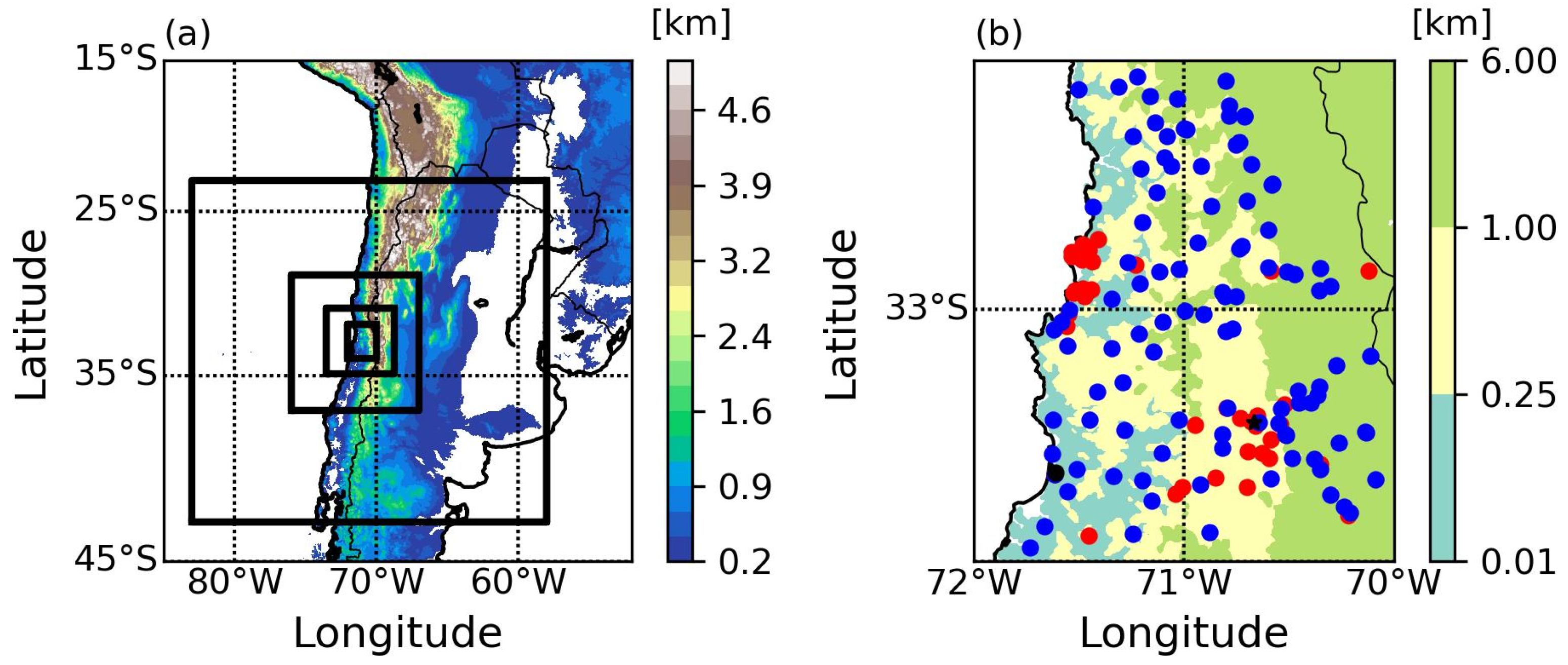
Figure 1.
(a) The WRF 4-nested domain configuration and (b) the location of atmospheric weather stations (red circles), the rain gauges (blue circles), and the Santo Domingo radiosonde station (black circle) superimposed on domain D4. The black star shows the location of Santiago’s center and the shaded colors represent the terrain altitude from D4, separated by the three ranges used to select coastal, interior valley, and mountainous locations in the study.
Figure 2.
Height–longitude cross-section of terrain height from Google Earth (∼0.44 km) and WRF domain 4 (1 km horizontal resolution) at the latitude −33.45° S. The black star represents the location of Santiago city.
Figure 2.
Height–longitude cross-section of terrain height from Google Earth (∼0.44 km) and WRF domain 4 (1 km horizontal resolution) at the latitude −33.45° S. The black star represents the location of Santiago city.
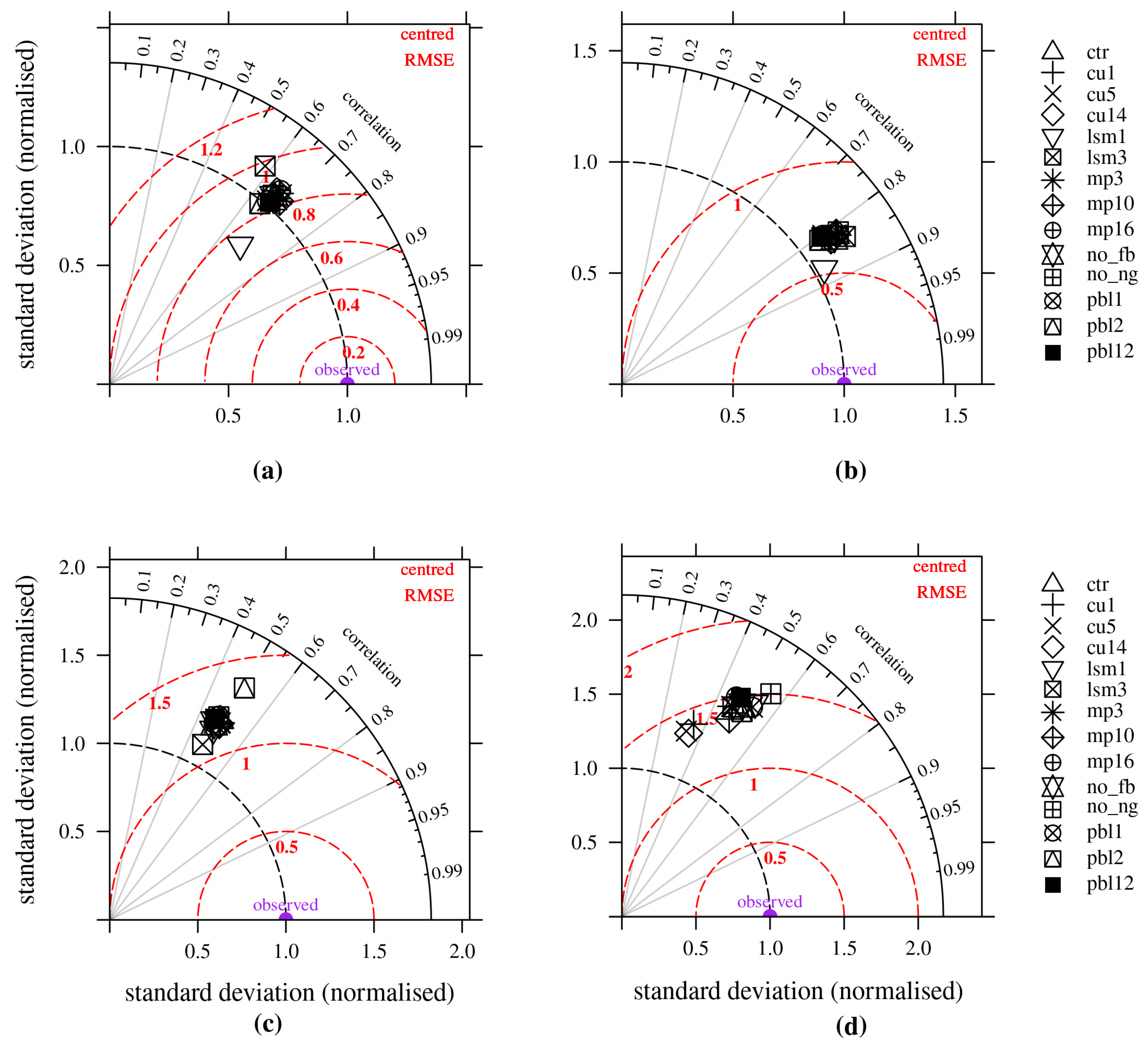
Figure 3.
Taylor diagrams of (a) 2 m RH, (b) 2 m temperature, (c) 10 m wind speed, and (d) daily accumulated precipitation for all simulations averaged over the whole domain and period of study. Diagrams include the normalized standard deviation (nsdev) on the x- and y-axis, the Pearson correlation coefficient along the azimuth, and the centered RMSE difference (radially from nsdev reference value 1).
Figure 4.
Mean (thick line) and standard deviation (thin line) profiles for the observed (black line) and simulated (a) temperature, (b) water vapor mixing ratio, and (c) wind speed. The blue and red lines on each panel show the simulations with the lowest and largest RMSE with the Santo Domingo radiosondes between 1 September and 14 October 2014. See the legend for details.
Figure 5.
Mean RMSE for (a) 2 m RH, (b) 2 m temperature, and (c) 10 m wind speed for each simulation for perturbed and unperturbed days over the domain of study. (d–f) Same as (a–c), but for the mean bias.
Figure 5.
Mean RMSE for (a) 2 m RH, (b) 2 m temperature, and (c) 10 m wind speed for each simulation for perturbed and unperturbed days over the domain of study. (d–f) Same as (a–c), but for the mean bias.
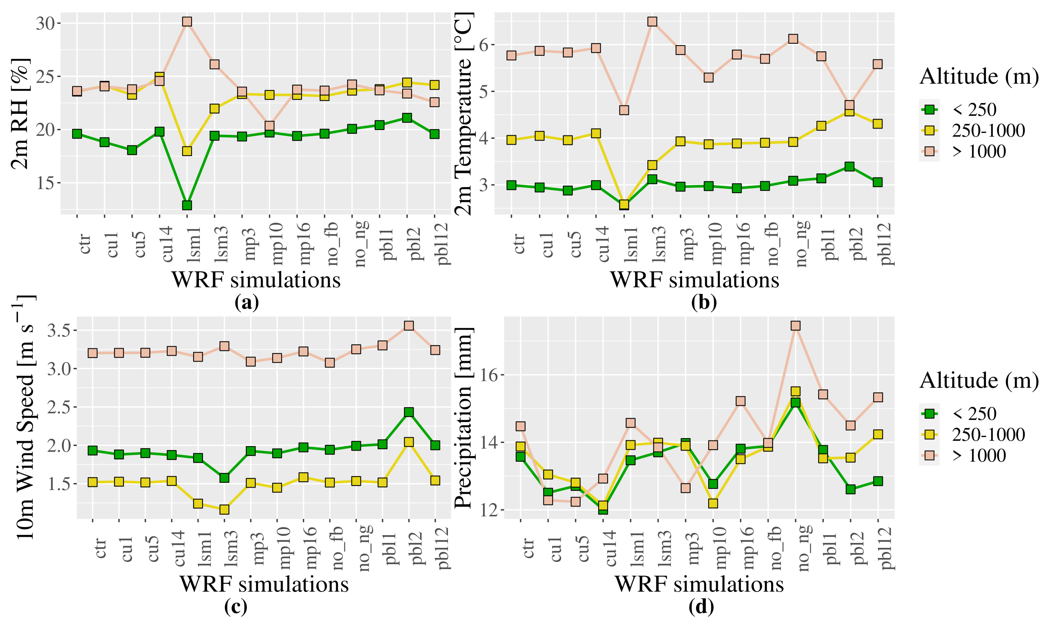
Figure 6.
The RMSE between WRF simulations and observations for (a) 2 m RH, (b) 2 m temperature, (c) 10 m wind speed, and (d) accumulated precipitation over each sub-region.
Figure 6.
The RMSE between WRF simulations and observations for (a) 2 m RH, (b) 2 m temperature, (c) 10 m wind speed, and (d) accumulated precipitation over each sub-region.
Figure 7.
Diurnal variation of (a) 2 m RH, (b) 2 m temperature, and (c) 10 m wind speed, averaged over the period of study and for each sub-region.
Figure 7.
Diurnal variation of (a) 2 m RH, (b) 2 m temperature, and (c) 10 m wind speed, averaged over the period of study and for each sub-region.
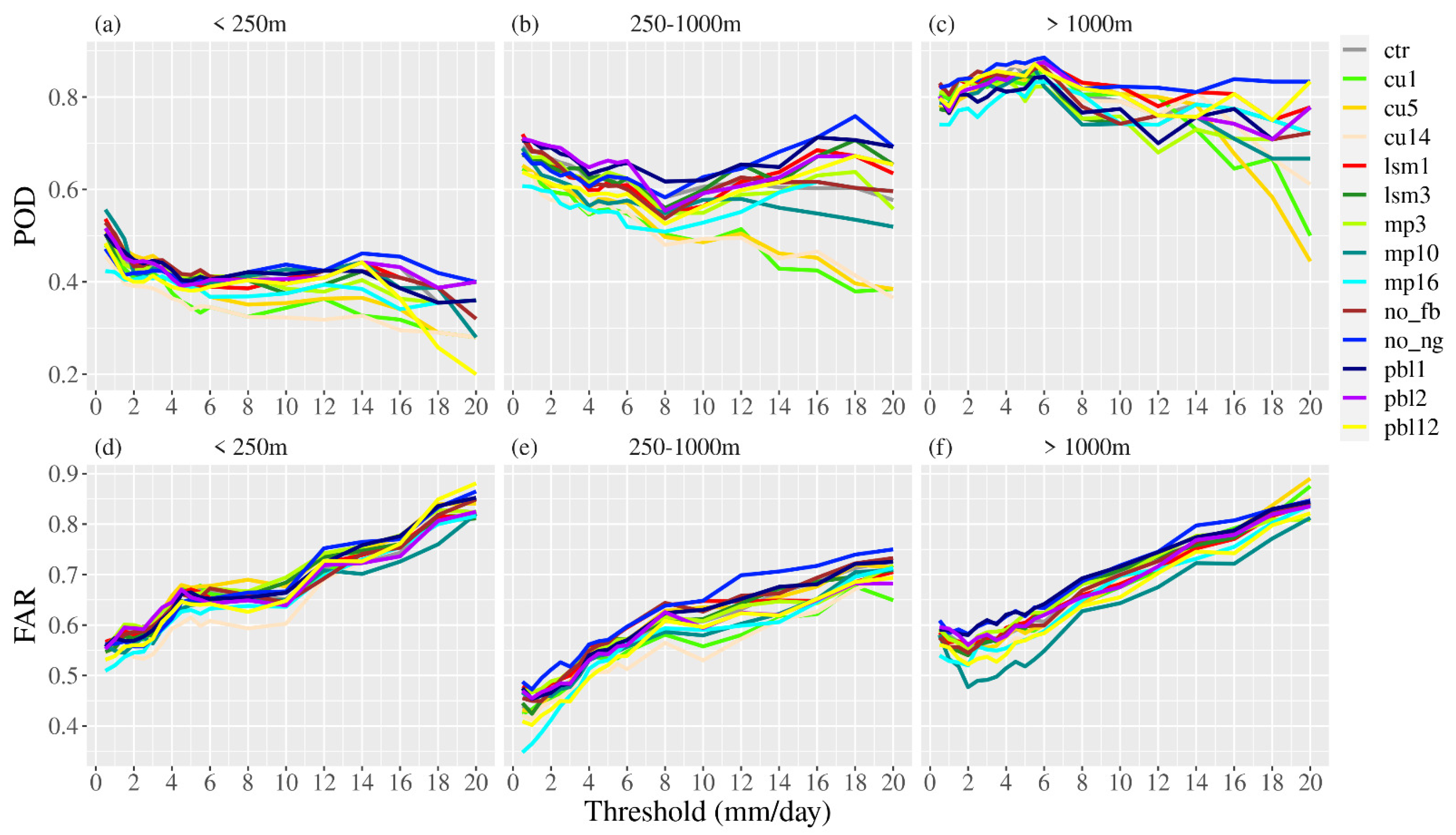
Figure 8.
Probability of detection (POD) as a function of rainfall threshold for all WRF simulations and for (a) coastal, (b) interior valleys, and (c) mountain locations over the period of study. (d–f) Same as (a–c), but for the false alarm ratio (FAR).
Figure 8.
Probability of detection (POD) as a function of rainfall threshold for all WRF simulations and for (a) coastal, (b) interior valleys, and (c) mountain locations over the period of study. (d–f) Same as (a–c), but for the false alarm ratio (FAR).
Figure 9.
Bias score (BS) as a function of rainfall threshold for all WRF simulations and for (a) coastal, (b) interior valleys, and (c) mountain locations over the period of study. (d–f) Same as (a–c), but for the critical success index (CSI).
Figure 9.
Bias score (BS) as a function of rainfall threshold for all WRF simulations and for (a) coastal, (b) interior valleys, and (c) mountain locations over the period of study. (d–f) Same as (a–c), but for the critical success index (CSI).
Figure 10.
Horizontal distributions of (a) PWV (color shaded), MSLP (white contours), geopotential height at 500 hPa (black contours), and wind vectors at 10 m, and (b) wind speed (color shaded), geopotential height (black contours), and wind vectors at 300 hPa for 6 August 2014 at 0000 UTC from ERA5 reanalysis. The black star shows the location of Santiago city.
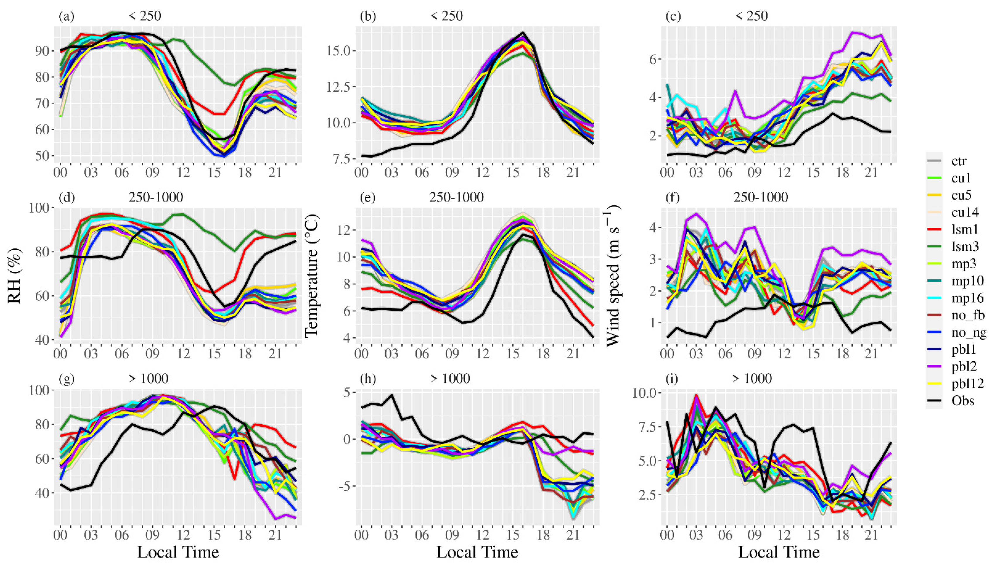
Figure 11.
Diurnal variation of (a) 2 m RH, (b) 2 m temperature, and (c) 10 m wind speed from WRF simulations and observations for 6 August 2014, averaged over coastal stations. (d–f) and (g–i) same as (a–c), but for interior valleys and mountain locations, respectively.
Figure 11.
Diurnal variation of (a) 2 m RH, (b) 2 m temperature, and (c) 10 m wind speed from WRF simulations and observations for 6 August 2014, averaged over coastal stations. (d–f) and (g–i) same as (a–c), but for interior valleys and mountain locations, respectively.
Figure 12.
Horizontal distribution of daily accumulated precipitation (shaded color) from (a) rain gauges, (b) IMERG data, (c) WRF cu14 simulation, and (d) WRF no_ng simulation for 6 August 2014. The black solid lines represent the terrain height (intervals every 1 km, starting at 1 km). The black star and circle show the locations of DGA Santiago and Pirque rain gauges, respectively.
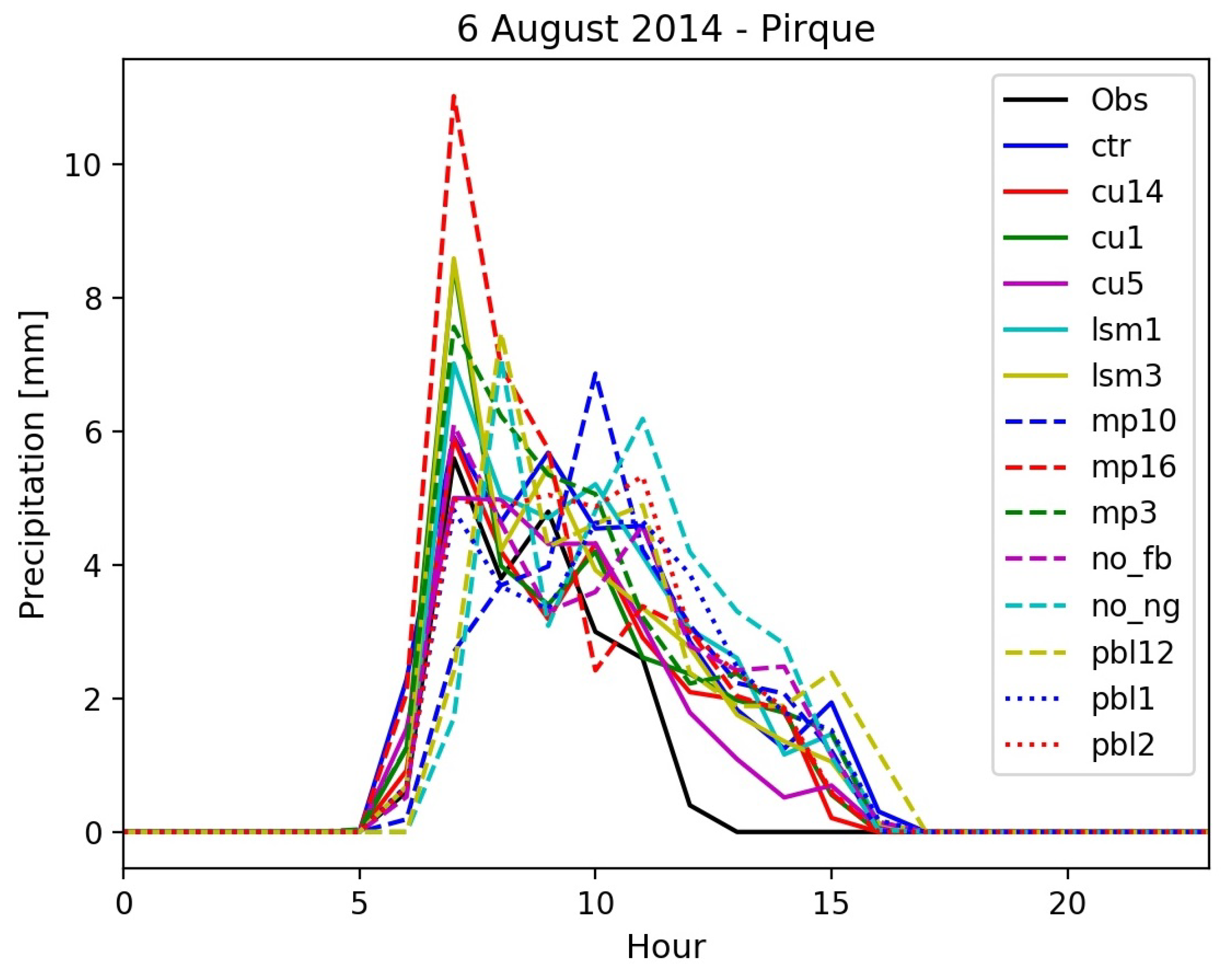
Figure 13.
Hourly precipitation from rain gauges and WRF simulations at Pirque station (33.6739° S, 70.58694° W, and 663 m height).
Figure 13.
Hourly precipitation from rain gauges and WRF simulations at Pirque station (33.6739° S, 70.58694° W, and 663 m height).
Figure 14.
(a) The temperature (color shaded) and wind field at 500 hPa, and the 1000–500 hPa thickness (contours), and (b) the wind speed (color shaded), geopotential height (contours), and wind vectors at 300 hPa for 13 September 2014 at 1200 UTC from ERA5 reanalysis. The white star shows the location of Santiago city.
Figure 15.
Same as
Figure 11, but for 13 September 2014.
Figure 15.
Same as
Figure 11, but for 13 September 2014.
Figure 16.
Horizontal distribution of daily accumulated precipitation (shaded color) from (a) rain gauges, (b) IMERG data, (c) WRF cu14 simulations, and (d) WRF no_ng simulation for 13 September 2014. The black solid lines represent the terrain height (intervals of 1 km, starting at 1 km). The black star shows the location of the DGA Santiago rain gauge.
Table 1.
Description of the configuration used in each of the 14 model runs. Changes with respect to the ctr simulation are highlighted in bold, depending on the land-surface model (LSM), microphysics (MP), cumulus, and planetary boundary layer (PBL) schemes employed, and the decision to use nudging or 1–2 feedback options.
| No. | Sim | LSM | PBL | Cumulus | MP | Nudging | Feedback |
|---|
| 1 | ctr | Noah | MYNN2 | Tiedtke | WSM6 | Yes | 2 way |
| 2 | cu1 | Noah | MYNN2 | KF | WSM6 | Yes | 2 way |
| 3 | cu5 | Noah | MYNN2 | Grell | WSM6 | Yes | 2 way |
| 4 | cu14 | Noah | MYNN2 | SAS | WSM6 | Yes | 2 way |
| 5 | lsm1 | 5L | MYNN2 | Tiedtke | WSM6 | Yes | 2 way |
| 6 | lsm3 | RUC | MYNN2 | Tiedtke | WSM6 | Yes | 2 way |
| 7 | mp3 | Noah | MYNN2 | Tiedtke | WSM3 | Yes | 2 way |
| 8 | mp10 | Noah | MYNN2 | Tiedtke | Morr | Yes | 2 way |
| 9 | mp16 | Noah | MYNN2 | Tiedtke | WTM6 | Yes | 2 way |
| 10 | no_fb | Noah | MYNN2 | Tiedtke | WSM6 | Yes | 1 way |
| 11 | no_ng | Noah | MYNN2 | Tiedtke | WSM6 | No | 2 way |
| 12 | pbl1 | Noah | YSU | Tiedtke | WSM6 | Yes | 2 way |
| 13 | pbl2 | Noah | MYJ | Tiedtke | WSM6 | Yes | 2 way |
| 14 | pbl12 | Noah | GBM | Tiedtke | WSM6 | Yes | 2 way |
Table 2.
Date and type of 14 perturbed days and the dates of 14 unperturbed days analyzed in this study.
Table 2.
Date and type of 14 perturbed days and the dates of 14 unperturbed days analyzed in this study.
| Date | Event |
|---|
| 5–6 August 2014 | Cold front |
| 22–24 August 2014 | Cold front |
| 29 August–5 September 2014 | Cold front |
| 13 September 2014 | Cut-off low |
| 9 August 2014 | Unperturbed |
| 12–15 August 2014 | Unperturbed |
| 18–20 August 2014 | Unperturbed |
| 26–27 August 2014 | Unperturbed |
| 11 September 2014 | Unperturbed |
| 15–17 September 2014 | Unperturbed |
Table 3.
Contingency table between the observed and simulated rainy events that defines the hits, misses, and false alarms for each specific threshold.
Table 3.
Contingency table between the observed and simulated rainy events that defines the hits, misses, and false alarms for each specific threshold.
| | Observed |
|---|
| | | Yes
| No
|
|---|
| Simulated | Yes | Hits | False alarms |
| | No | Misses | Correct non-events |
Table 4.
The RMSE, bias, and Spearman’s rank correlation coefficient () between each simulation and the observed 2 m RH and temperature, and the 10 m wind speed, averaged over the whole domain and the period of study. The simulations with the lowest value for RMSE, bias, and the highest rank correlation coefficient for each variable are shown in boldface.
| | RH | Temperature | Wind Speed |
|---|
| Sim | RMSE | Bias | ρ | RMSE | Bias | ρ | RMSE | Bias | ρ |
|---|
| ctr | 22.4 | −13.2 | 0.7 | 3.9 | 1.6 | 0.8 | 1.9 | 0.9 | 0.4 |
| cu1 | 22.6 | −13.2 | 0.7 | 3.9 | 1.6 | 0.8 | 1.9 | 0.8 | 0.4 |
| cu5 | 21.8 | −12.1 | 0.7 | 3.9 | 1.5 | 0.8 | 1.9 | 0.8 | 0.4 |
| cu14 | 23.4 | −14.3 | 0.7 | 4.0 | 1.7 | 0.8 | 1.9 | 0.8 | 0.4 |
| lsm1 | 18.0 | 8.5 | 0.7 | 2.8 | −0.2 | 0.9 | 1.8 | 0.6 | 0.4 |
| lsm3 | 21.6 | −4.7 | 0.6 | 3.7 | 1.1 | 0.8 | 1.6 | 0.4 | 0.4 |
| mp3 | 22.2 | −13.0 | 0.7 | 3.9 | 1.5 | 0.8 | 1.9 | 0.8 | 0.4 |
| mp10 | 22.0 | −13.1 | 0.7 | 3.8 | 1.5 | 0.8 | 1.9 | 0.8 | 0.4 |
| mp16 | 22.2 | −12.2 | 0.7 | 3.8 | 1.4 | 0.8 | 1.9 | 0.9 | 0.4 |
| no_fb | 22.2 | −12.7 | 0.7 | 3.8 | 1.5 | 0.8 | 1.9 | 0.8 | 0.4 |
| no_ng | 22.7 | −13.3 | 0.7 | 3.9 | 1.5 | 0.8 | 1.9 | 0.9 | 0.4 |
| pbl1 | 22.8 | −13.8 | 0.6 | 4.1 | 2.0 | 0.8 | 2.0 | 1.0 | 0.4 |
| pbl2 | 23.3 | −14.7 | 0.6 | 4.2 | 2.4 | 0.8 | 2.4 | 1.4 | 0.5 |
| pbl12 | 22.7 | −14.0 | 0.7 | 4.1 | 2.0 | 0.8 | 2.0 | 0.9 | 0.4 |
Table 5.
The RMSE, bias, and Spearman’s rank correlation coefficient () for the daily accumulated precipitation (>1 mm) between each simulation and observations, averaged over the whole domain and the period of study. The simulation with the lowest value of RMSE and bias, and the highest rank correlation coefficient, is shown in boldface.
| | Precipitation |
|---|
| Sim | RMSE | Bias | ρ |
|---|
| ctr | 15.3 | 7.5 | 0.4 |
| cu1 | 13.7 | 4.2 | 0.3 |
| cu5 | 13.5 | 4.5 | 0.3 |
| cu14 | 13.1 | 3.7 | 0.4 |
| lsm1 | 15.2 | 7.4 | 0.4 |
| lsm3 | 15.3 | 7.5 | 0.4 |
| mp3 | 14.8 | 6.4 | 0.4 |
| mp10 | 13.6 | 5.2 | 0.4 |
| mp16 | 16.0 | 7.4 | 0.4 |
| no_fb | 15.0 | 7.3 | 0.4 |
| no_ng | 18.1 | 11.4 | 0.5 |
| pbl1 | 15.4 | 8.3 | 0.4 |
| pbl2 | 14.6 | 7.0 | 0.4 |
| pbl12 | 15.9 | 7.7 | 0.4 |
Table 6.
The RMSE and bias for 2 m temperature (temp), 2 m RH, 10 m wind speed (Wsp), and the daily accumulated precipitation (values > 1 mm), averaged over all simulations, for each sub-region of central Chile.
Table 6.
The RMSE and bias for 2 m temperature (temp), 2 m RH, 10 m wind speed (Wsp), and the daily accumulated precipitation (values > 1 mm), averaged over all simulations, for each sub-region of central Chile.
| | RMSE | Bias |
|---|
| Variable | <250 m | 250–1000 m | >1000 m | <250 m | 250–1000 m | >1000 m |
|---|
| 2 m RH (%) | 19.1 | 23.2 | 24.1 | −9.8 | −14.8 | 9.1 |
| 2 m Temp (°C) | 3.0 | 3.9 | 5.7 | 1.1 | 2.5 | −3.4 |
| 10 m Wind Speed (ms−1) | 1.9 | 1.5 | 3.2 | 1.1 | 0.7 | −0.4 |
| Precipitation (mm) | 13.4 | 13.6 | 14.3 | −1.9 | 1.5 | 5.9 |
Table 7.
RMSE and bias of daily accumulated precipitation for cu14 and no_ng simulations over each sub-region for 6 August 2014 and 13 September 2014 study cases.
Table 7.
RMSE and bias of daily accumulated precipitation for cu14 and no_ng simulations over each sub-region for 6 August 2014 and 13 September 2014 study cases.
| | | RMSE | Bias |
|---|
| Day | Sim | <250 m | 250–1000 m | >1000 m | <250 m | 250–1000 m | >1000 m |
|---|
| 6 August 2014 | cu14 | 13.9 | 8.9 | 10.5 | 10.8 | 6.2 | 9.3 |
| 6 August 2014 | no_ng | 17.5 | 11.4 | 11.2 | 14.6 | 9.2 | 9.8 |
| 13 September 2014 | cu14 | 4.8 | 8.5 | 7.8 | −2.5 | −2.3 | −0.6 |
| 13 September 2014 | no_ng | 5.2 | 8.7 | 11.8 | −3.2 | −5.2 | 2.9 |

 ,
, 


