
The Reexamination of the Moisture–Vortex and Baroclinic Instabilities in the South Asian Monsoon
1
Key Laboratory of Meteorological Disaster, Ministry of Education (KLME)/Joint International Research Laboratory of Climate and Environmental Change (ILCEC)/Collaborative Innovation Center on Forecast and Evaluation of Meteorological Disasters (CIC-FEMD), Nanjing University of Information Science and Technology, Nanjing 210044, China
2
Department of Atmospheric Sciences, School of Ocean and Earth Science and Technology, University of Hawaii at Manoa, Honolulu, HI 96822, USA
*
Author to whom correspondence should be addressed.
Atmosphere 2024, 15(2), 147; https://doi.org/10.3390/atmos15020147
Submission received: 20 December 2023
/
Revised: 20 January 2024
/
Accepted: 22 January 2024
/
Published: 24 January 2024
(This article belongs to the Section Meteorology)
Abstract
:Observational analyses reveal that a dominant mode in the South Asian Monsoon region in boreal summer is a westward-propagating synoptic-scale disturbance with a typical wavelength of 4000 km that is coupled with moistening and precipitation processes. The disturbances exhibit an eastward tilt during their development before reaching their maximum activity center. A 2.5-layer model that extends a classic 2-level quasi-geostrophic model by including a prognostic lower-tropospheric moisture tendency equation and an interactive planetary boundary layer was constructed. The eigenvalue analysis of this model shows that the most unstable mode has a preferred zonal wavelength of 4000 km, a westward phase speed of 6 m s−1, an eastward tilt vertical structure, and a westward shift of maximum moisture/precipitation center relative to the lower-tropospheric vorticity center, all of which agree with the observations. Sensitivity experiments show that the moisture–vortex instability determines, to a large extent, the growth rate, while the baroclinic instability helps set up the preferred zonal scale. Ekman-pumping-induced vertical moisture advection prompts an in-phase component of perturbation moisture relative to the low-level cyclonic center, allowing the generation of available potential energy and perturbation growth, regardless of whether or not a low-level mean westerly is presented. In contrast to a previous study, the growth rate is reversely proportional to the convective adjustment time. The current work sheds light on understanding the moisture–vortex and the baroclinic instability in a monsoonal environment with a pronounced easterly vertical shear.
1. Introduction
The South Asian summer monsoon (SASM) is a major circulation system in the Northern Hemisphere in boreal summer. It is characterized by an annual reversal of prevailing wind and a strong contrast of a wet and a dry season [1,2,3,4,5]. The monsoon rain impacts the lives of more than one billion people [6,7,8,9,10,11]. The low-level circulation over the SASM is characterized by zonally oriented westerly winds from the Arabian Sea all the way to the South China Sea. Accompanied with the low-level westerly jet (LLJ) is intense convection and precipitation along the 10–20° N latitudinal zone and northward cross-equatorial flow [12,13,14,15,16,17].
A unique feature of the SASM, compared to the other regions of the globe, is the positive meridional gradient of the mean temperature and moisture, that is, the mean temperature and moisture increase with latitude [6,18,19,20,21,22]. As a consequence, there is a pronounced background easterly vertical shear in the region [2,19,22,23,24,25]. Under such background conditions, synoptic-scale waves or disturbances with intense precipitation often develop in this region [20,26,27,28]. Some of the disturbances grow into the tropical cyclone category [2,29,30,31,32,33]. These disturbances move northwestward, causing devastating floods in South Asia [14,20,34].
The occurrence of the dominant synoptic-scale variability over the SASM region requires further theoretical understanding of the physical mechanisms behind the observational phenomenon. The classic baroclinic instability theory clearly explains the preferred wavelength, phase propagation, and energy source of the dominant synoptic perturbations in mid-latitudes during boreal winter [35,36,37,38,39,40,41]. Without the involvement of diabatic heating processes, the winter synoptic-scale perturbations may gain energy directly from the mean kinetic and potential energy, as demonstrated by a two-level model under a constant background vertical shear [37,41].
The development of boreal summer synoptic-scale disturbances over the SASM region differs significantly from the classic baroclinic instability (BI) theory in the following perspectives. Firstly, moistening and condensational heating processes become critical so that the diabatic heating effect cannot be ignored. Secondly, the background vertical shear and meridional gradients of temperature and specific humidity reverse their signs so that processes through which perturbation-available potential energy is generated differ. This prompted earlier studies of a moist baroclinic instability (Shukla 1978, Mak 1983) [42,43] that linked diabatic heating to mid-tropospheric vertical motion induced by quasi-geostrophic (QG) dynamics. The key assumption behind the earlier moist BI theory was the direct link of diabatic heating to QG lifting-induced advection of mean moisture so that perturbation moisture and its tendency were neglected. A necessary condition for the dry or moist BI to work is an upshear tilt vertical structure, but such a tilt was not observed in monsoon depressions (MDs), as demonstrated in Cohen and Boos (2016) [44].
Another potential mechanism in the SASM is a moist barotropic instability. The classic barotropic instability theory requires a sign reversal of meridional gradient of absolute vorticity () (Kuo 1949) [45]. While the realistic background flow in the SASM does not satisfy the barotropic instability criterion, a coupling between moisture and convection may provide additional energy for a perturbation to grow, as demonstrated by Diaz and Boos (2019) [46], using an anomaly atmospheric model. A least damped mode with a preferred perturbation structure was first stimulated by dry dynamics, and the perturbation became unstable and grew when the moisture–convection–circulation feedback kicked in. However, how a preferred wavelength was selected due to the moist barotropic instability is unclear. Nevertheless, the moist barotropic instability could serve as a potential mechanism for understanding the preferred variability of the SASM.
The third possible mechanism in the SASM is the moisture–vortex instability (MVI). This theory was first proposed by Adames and Ming (2018) [47] using a shallow water model. A caveat of the simple theoretical work is the inconsistency in specified background mean fields. While a background meridional temperature gradient is specified, its associated vertical shear is not presented so that the background state is not in a thermal wind balance. Adames (2021) [48] corrected this problem by constructing a two-level QG model with consistent background vertical shear and meridional temperature gradient fields. A key process for the MVI to work in Adames (2021) [48] was anomalous zonal moisture advection by low-level mean westerly, which shifted meridional advection generated moisture anomalies eastward toward the low-level cyclonic center, so that there was an in-phase component of perturbation moisture with low-level vorticity. Without this zonal advection, perturbation moisture and vorticity would be in a quadrature phase relation, which would lead to no instability. The unstable development of a synoptic-scale wave train in the tropical western North Pacific due to the convection-vortex feedback was demonstrated in Li (2006) [49] under a low-level easterly background condition. The cause of the instability lies on positive feedback between low-level cyclonic vortex and condensational heating induced by Ekman-pumping-induced boundary-layer moisture convergence. This poses the question of whether or not the presence of low-level westerly is a necessary background condition for the MVI to operate.
It has been shown that the vertical profile of anomalous vertical velocity evolves at different phases of convection development. For example, in front of a MJO center, perturbation moisture first develops in the lower troposphere due to PBL convergence (Hsu and Li 2012) [50]. At this phase, a major moistening process is Ekman-pumping-induced vertical advection, while mid-tropospheric vertical motion is weak. Later, shallow convection develops into deep convection, and at that phase, maximum ascent appears in the mid-troposphere. Given that the mean moisture decreases rapidly with height with a typical e-folding scale of 2.2 km (Wang and Li 1993) [51], Ekman-pumping-induced vertical advection at the top of the planetary boundary layer (PBL) should play a critical role in affecting lower-tropospheric moistening. However, such a process was omitted in Adames (2021) [48]. Instead, the vertical advection in Adames (2021) [48] was controlled by a mid-tropospheric vertical motion. By assuming that low-level vertical velocity is in phase with mid-tropospheric vertical velocity (with a reduced amplitude), Adames (2021) [48] implicitly assumed that a mid-tropospheric ascent would lead to a positive vertical advection of moisture in the lower troposphere. Consider a flux form of moisture transport in the lower tropospheric box. At the base of the box, Ekman-pumping-induced ascent transports moisture from the PBL into the box, increasing the moisture in the box. At the top of the box, an ascent in the mid-troposphere tends to transport moisture out of the box, decreasing the moisture in the box. Thus, caution is needed to link the lower-tropospheric moisture tendency to the mid-tropospheric ascent.
An odd result in Adames (2021) [48] is the increase of the MVI with an increased convective adjustment time. This is unphysical because, given the same low-level vortex, the moisture tendency is determined (because it is primarily controlled by advective processes), and the same moisture would lead to greater precipitation and thus greater convection–circulation feedback and instability for a given smaller adjustment time.
The controversial issues above motivated us to re-examine the MVI and the BI in a more suitable model framework that contains an interactive PBL and Ekman-pumping-induced moisture advection. To validate the MVI and BI theories, an observational analysis is carried out. While previous observational validations focused on MDs (e.g., Cohen and Boos 2016) [44], here we examine the structure and evolution characteristics of general synoptic-scale perturbations, including tropical waves.
The remaining part of this paper is organized as follows: A brief description of the data and the model is given in Section 2. Section 3 describes the observed characteristics of the background mean state and synoptic-scale disturbances in boreal summer over the SASM region. Special attention is paid to revealing the spatial phase relationships among the perturbation moisture, precipitation, and circulation. The construction of a 2.5-layer QG model with a prognostic moisture equation and its eigenvalue solutions are described in Section 4. In Section 5, we discuss a few special issues relevant to the MVI and BI. Finally, a conclusion is presented in the last section.
2. Data and Model
A daily interpolated outgoing longwave radiation (OLR) product obtained from the National Oceanic and Atmospheric Administration (NOAA) polar-orbiting satellites [52] was used in this study. The OLR field reflects atmospheric convection and precipitation over the South Asian Monsoon region [5]. The OLR dataset spans from 1979 to 2016, at a horizontal resolution of 1.0° × 1.0°.
In addition, we employed the European Center for Medium-Range Weather Forecasts (ECMWF) Re-Analysis 5 (ERA5; [53]). This dataset is interpolated into a horizontal resolution of 1.0° × 1.0° with 12 pressure levels to match the OLR product. The reanalysis dataset contains zonal and meridional wind fields (u, v), specific humidity (q), air temperature (T), and geopotential height () from 1979 to 2016. This dataset is used to reveal the structure and evolution characteristics of synoptic-scale disturbances in the South Asian monsoon region.
As we focus on the boreal summer season, our analyses are confined to the period from June to August. The synoptic-scale fields were derived by applying a 10-day high-pass filter to the original datasets. The climatological annual cycle was removed first from the original data before the temporal decomposition was applied.
A 2.5-layer QG theoretical model is constructed, following Adames (2021) [48] and Yang and Li (2023) [54]. The model was an extension of a conventional 2-level QG model [41] by including a prognostic lower-tropospheric moisture tendency equation and a well-mixed PBL that interacts with the free-atmospheric circulation [51]. In the current model, the reference latitude is set to be 16° N. For a detailed derivation of the model equations and methodology to solve the equations, readers are referred to Yang and Li (2023) [54] as well as Section 4.
3. Observed Characteristics of the Background Field and Synoptic-Scale Variability in the SASM
3.1. Background Field Features
The summer mean circulation in the South Asian monsoon region is characterized by an enhanced rainfall belt along the monsoon trough zone (10–20° N latitudinal band), pronounced low-level westerlies, and an upper-tropospheric easterly jet [12,13,14,15,16,17,22,23]. Figure 1a displays the summer climatological mean Outgoing Longwave Radiation (OLR) and 850-hPa wind fields. It can be discerned from this figure that the minimum centers of the OLR field [i.e., the dark blue region (10–20° N, 60–120° E)] represents the region of intense convection, which is a key region of the South Asian monsoon. Along the intense convective zone, there are three prominent centers elongated from east to west, the South China Sea, the Bay of Bengal, and the western Arabian Sea.
Accompanying the convective zone is the marked westerly wind at 850 hPa. The low-level westerlies originate from the Southern Hemisphere, linked with southeasterly trades south of the equator and northward cross-equatorial flow. The equatorially antisymmetric flow is part of a large-scale monsoon circulation driven by the hemispherically asymmetric solar radiative forcing in northern summer.
The upper-tropospheric jet is a unique feature of the global atmosphere. While the westerly jet is pronounced in middle latitudes, being consistent with a southward temperature gradient in the northern hemisphere, the easterly jet over the South Asia monsoon region implies a northward temperature gradient according to the thermal wind relation. This implies that the temperature increases with increased latitude in the region, which is rarely seen in other parts of the globe. Thus, the easterly vertical shear stands out as a prominent characteristic of the South Asian monsoon (Figure 1b), distinguishing itself from other tropical regions and higher latitudes. Here, the vertical wind shear is computed by the subtraction of the zonal wind component of the climatological 850-hPa wind field from the zonal wind component of the climatological 200-hPa wind field. The Bay of Bengal and the Arabian Sea are identified as the primary regions characterized by maximum easterly vertical shear, with a maximum value of about −30 m s−1.
Another unique feature of the South Asian monsoon is the increase of the background mean-specific humidity with latitude, setting it apart from other parts of the globe. Figure 1c depicts the climatological mean-specific humidity field in boreal summer at 925-hPa. The figure clearly indicates that the South Asian monsoon is the region of maximum specific humidity, which provides favorable conditions for the development of tropical disturbances. Over the Bay of Bengal, the Arabian Sea, and the South China Sea, there is a distinct increasing trend of specific humidity from south to north, with a maximum value of about 20 g kg−1 around 20° N.
Similar to the moisture field, the vertically integrated temperature from either 850 hPa to 200 hPa or 500 hPa to 200 hPa shows a northward increasing trend over the South Asian monsoon region (Figure 1d). The increased temperature results primarily from the condensational heating along the monsoon trough zone. It is in the thermal wind relation with the easterly vertical shear in the region.
3.2. Dominant Variability
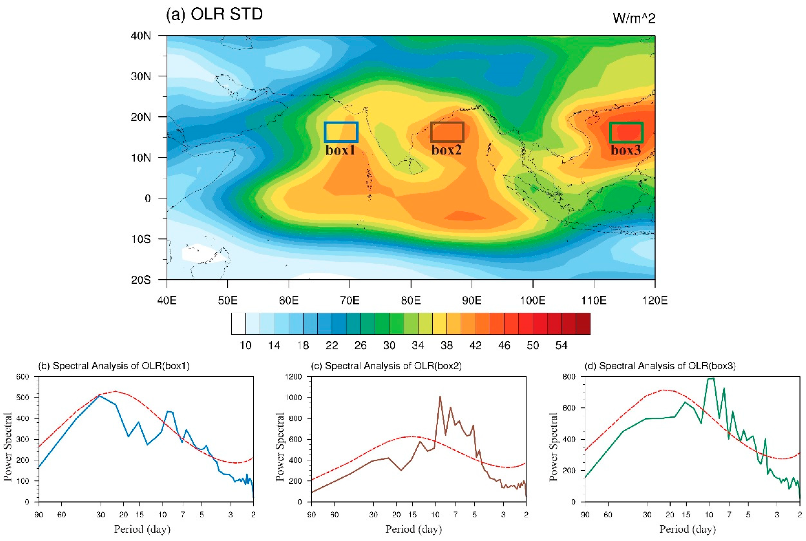
To illustrate the variability centers over the South Asian monsoon region, we plotted the standard deviation map of the daily OLR field for the period of 1979–2016. Along the climatological mean convective zone (10–20° N), three significant OLR variability centers are identified. They are located over the Arabian Sea, Bay of Bengal, and the South China Sea, respectively. The three centers are labeled as box1, box2, and box3, as shown in Figure 2a.
To reveal the dominant periods of the OLR variability over the Arabian Sea, Bay of Bengal, and the South China Sea, we conduct a power spectral analysis for the averaged OLR anomalies over box1, box2, and box3, and the results are illustrated in Figure 2b–d. In these figures, solid curves with different colors represent the power spectrum over the corresponding boxes, while the dashed red curves denote the 95% confidence level. A common feature among the three regions is a dominant period of below 10 days, indicating that the dominant perturbations in the region are synoptic-scale disturbances. The resemblance in the power spectral features across the three regions suggests that synoptic-scale signals across the regions might be physically linked, representing a zonally propagating mode. It also implies that the dynamic origin of the synoptic-scale disturbances in the regions may arise from the same instability mechanism.
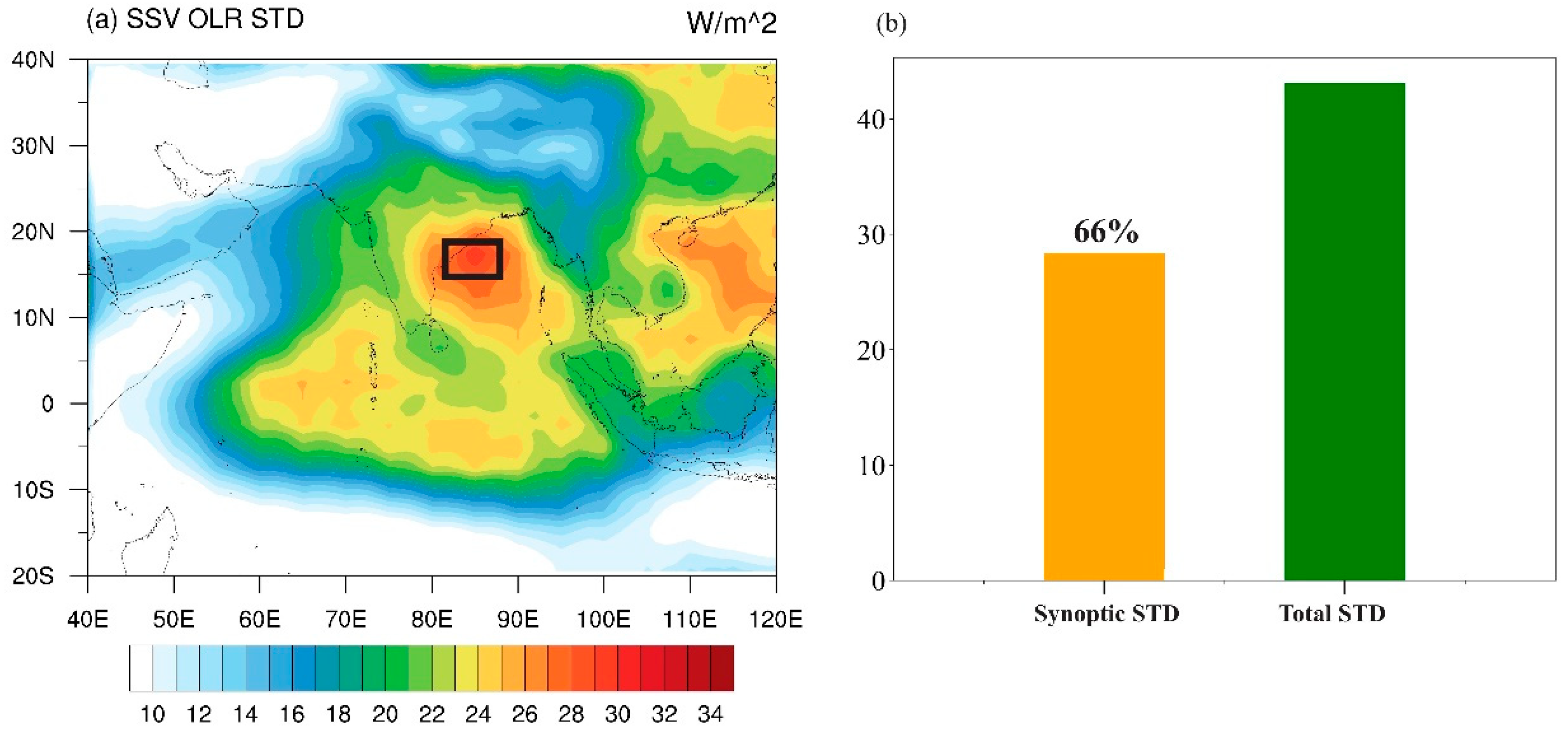
To clearly illustrate the dominance of the synoptic-scale variability, we plotted the standard deviation map of 10-day high-pass filtered OLR field. As seen in Figure 3a, the synoptic-scale variability exhibits a maximum center over the northern part of the Bay of Bengal (10–20° N, 80–90° E), with a second maximum center over the South China Sea. To quantitatively measure the relative contribution of the synoptic-scale variability to the total variability, we computed the ratio of the area-averaged standard deviation of the synoptic-scale OLR signal to the total standard deviation in the Bay of Bengal (14–18° N, 83–87° E). As shown in Figure 3b, the synoptic-scale OLR variability constitutes 66% of the total variability. In other words, the synoptic-scale disturbances are indeed the dominant perturbations in the South Asian monsoon region. Therefore, in the subsequent analysis, we focus on examining the structure and evolution characteristics of the synoptic-scale disturbances in this region.
3.3. The Evolving Horizontal Patterns and Vertical Structure
Figure 4 illustrates the temporally evolving patterns of the synoptic-scale OLR, 700-hPa specific humidity, 850 hPa geopotential height and 850 hPa wind fields regressed onto the synoptic-scale OLR time series averaged in the reference region (14–18° N, 83–87° E) (the black box shown in Figure 3a) from day −2 to day 0, the synoptic-scale disturbance shows a clear westward-propagating feature. In the journey of the westward movement, the synoptic disturbance steadily intensifies prior to day 0. A low-level cyclonic anomaly is accompanied by a negative geopotential height anomaly, exhibiting a quasi-geostrophic nature. The maximum specific humidity and minimum OLR centers are located to the west of the low-level cyclonic center. Given that OLR is a good indicator of convective activity [52], one may regard a minimum OLR center as a maximum convective center.
At day −2, a maximum convective center (yellow dot) is located approximately at 13° N, 95° E, with a high-pressure (anticyclonic) center prevailing to its west and a low-pressure (cyclonic) center appearing to its east. The anticyclone to the west and the cyclone to the east promote conspicuous northerly winds in between, leading to a positive moisture advection in situ and, thus, the increase of local specific humidity. As shown in Figure 4d, a positive specific humidity anomaly appears at 15° N, 100° E (Figure 4a,d).
At day −1, the maximum convective center moves to 15° N, 88° E. Similar to the OLR, anomalous wind, the geopotential height and specific humidity fields all exhibit westward phase propagation. The positive specific humidity anomaly appears at 18° N, 90° E, somewhere between the high- and low-pressure centers (Figure 4b,e). Considering the northward background-specific humidity gradient (depicted in Figure 1c), northerly winds to the west of the low-level cyclone advect higher mean moisture southward, favoring a low-tropospheric moistening and the strengthening of convection.
At day 0, the synoptic-scale disturbance reaches its maximum as both the convective center and the specific humidity center move to near 18° N, 85° E (Figure 4c,f). Meanwhile, the low-pressure system to their east also attains maximum amplitude, accompanied by a strong cyclonic circulation.
One may estimate the zonal phase speed of the developing synoptic-scale disturbance based on the OLR evolution shown in Figure 4. Our calculation shows that the approximate westward propagation speed is 6 m s−1. The half-wavelength of the synoptic-scale disturbance may also be estimated based on the zonal distance between the high- and low-pressure centers shown in Figure 4. Our calculation shows that the wavelength is approximately 4000 km.
After revealing the horizontal structure, next, we examine the vertical structure of the synoptic-scale disturbances. Figure 5 illustrates the zonal-vertical cross-sections of the synoptic-scale specific humidity and geopotential height fields averaged over 16–18° N from day −2 to day 0. As shown in Figure 3, the maximum synoptic-scale variability center appears at a longitudinal zone of 83–87° E. Thus, the developing phase of the synoptic perturbations should be confined to the east of this zone. Figure 5 shows that to the east of 95° E, the geopotential height anomaly field exhibits an eastward tilting vertical structure during the developing period from day −2 to day 0. This upshear tilt was also seen in Luo et al. (2023) [55] (e.g., in their Figure 5). Such an upshear tilt implies a possible role of dry or moist BI during the perturbation development. The upshear tilt becomes less apparent as the disturbance moves to or near the maximum variability center. The growth of the disturbance can be inferred from the rapid increase of specific humidity anomalies from day −2 to day 0 (Figure 5).
To sum up, the observational analysis above reveals that the synoptic-scale disturbances are the most dominant mode in the SASM region. They are characterized by a westward phase speed of 6 m s−1, a zonal wavelength of 4000 km, and a strong coupling among circulation, moisture, and convection. An eastward tilt is observed to the west of the maximum activity center. While the perturbation moisture and convection are approximately in phase, they are located to the west of the low-level cyclonic center. In the following section, we intend to construct a theoretical model to understand the preferred wavelength, phase speed, and horizontal and vertical structures of the observed synoptic-scale disturbances over the SASM region.
4. Construction of a 2.5-Layer Model and Eigenvalue Solutions
Given the unique feature of the South Asian monsoon with pronounced easterly vertical shear and northward meridional temperature and moisture gradients, we constructed a 2.5-layer model in a way similar to Yang and Li (2023) [54]. This model involves both the QG dynamics [41] and moistening and condensational heating processes. The model contains a 2-level free atmosphere and a well-mixed PBL.
As shown in Figure 6, the model vertical levels 0, 1, 2, 3, and 4 denote, respectively, the top of the atmosphere, the upper troposphere, the middle troposphere, the lower troposphere, and the top of PBL. Assume that the vertical velocity vanishes at the top and the bottom. At the top of PBL, the Ekman-pumping-induced vertical velocity is determined by relative vorticity in the lower troposphere, and it can be expressed as
where represents the Ekman pumping coefficient.
The vorticity equations are written at levels 1 and 3 as follows:
where is the pressure interval between level 1 and 3 (or between level 0 and 2), and the subscript notation is used to designate the vertical level.
Term at level 2 may be estimated using the following formula:
Thus, the thermodynamic equation at level 2 can then be expressed as follows:
Following Adames and Ming (2018) [47] and Adames (2021) [48], a simplified Betts–Miller scheme is used, that is, perturbation precipitation is proportional to low-level specific humidity but is oppositely proportional to a convective adjustment time (see Equation (6)). Therefore, perturbation diabatic heating in the middle troposphere may be expressed as a function of precipitation anomaly, that is,
where and represents the convective adjustment time.
By combining the QG vorticity and thermodynamics equations with a lower-tropospheric specific humidity equation, one may derive a close set of linearized governing equations with three dependent variables, barotropic and baroclinic stream-function fields and lower-tropospheric specific humidity field, as follows:
where , , , , and ; denotes the vertically averaged mean flow, and denotes the background vertical shear; represents the mid-tropospheric perturbation stream-function, and is proportional to the mid-tropospheric perturbation temperature. For more detailed derivations of the equations above, readers are referred to Yang and Li (2023) [52].
Considering wave-like solutions for Equations (9)–(11) with the following forms:
where A, B, and C represent the amplitude, k denotes zonal wavenumber, i = (−1)1/2, and real and imaginary parts of c relate to phase speed and growth rate, respectively. By substituting the wave-like solutions into the governing Equations (9)–(11), one may derive a dispersion equation and obtain eigenvalue solutions with the use of Newton’s iterative method. The key control parameters used in the current model are listed in Table 1. These parameter values are derived from observational analyses (e.g., Figure 1).
Figure 7 shows the eigenvalue solution with the use of the control parameter values. It shows the growth rate (kci) and phase speed (cr) as a function of zonal wavenumber (k). It is interesting to note that the growth rate peaks at 4000 km. This implies that the most unstable mode in the South Asian monsoon region is the synoptic-scale perturbation with a typical wavelength of 4000 km. This result is in good agreement with the observational analysis shown in Section 3. The wavelength derived from the current model is roughly twice as large as that derived from Adames (2021). Similar to the classic BI theory, the most unstable mode prefers an intermediate-length scale, while both long and short-length scales are unfavorable. The maximum growth rate is 13 × 10−6 s−1 (Figure 7a), which corresponds to an e-folding scale of about one day, being proper for the development of the synoptic-scale disturbances. The zonal westward phase speed of the most unstable mode is about 6 m s−1 (Figure 7b). Again, this agrees with the observations.
The zonal phase structures of three dependent variables of the moist baroclinic model for the most unstable mode are illustrated in Figure 8. Note that the perturbation baroclinic stream-function lags approximately 90° behind the perturbation barotropic stream-function . Meanwhile, the perturbation specific humidity () is approximately zonally in phase with .
Under the QG regime, the perturbation geopotential height is proportional to the following perturbation stream-function:
and the following hydrostatic equation:
implies that the perturbation baroclinic stream-function is proportional to perturbation temperature ().
The growth mechanisms in the current framework may be understood through the following qualitative analysis of perturbation available potential energy equation. The perturbation thermodynamic equation may be written as follows:
Multiplying at both sides of the equation, we have the following:
where the term at the left-hand side is proportional to the tendency of available potential energy (APE); the first term in the right-hand side represents the APE generation due to the conversion from the mean APE, a main process for perturbation growth under the classic BI theory; and the second term in the right-hand side represents the APE generation due to condensational heating. A tilted bar represents phase integration within a complete phase cycle (i.e., 0–360°).
Given the in-phase relationship between perturbation specific humidity and diabatic heating , Figure 8 clearly indicates that and are positively correlated, that is as follows:
Because the classic BI theory did not consider the diabatic heating, here we demonstrate that the moistening and precipitation process is critical in affecting the growth rate over the SASM. Another noted feature from Figure 8 is the out-of-phase relation between mid-tropospheric perturbation meridional wind () and . Because is proportional to the zonal gradient of , a minimum of is located to the east of the maximum. As a result, the following is true:
In the classic BI theory, a positive correlation between and corresponds to the generation of perturbation APE, because the mean meridional temperature gradient in the middle latitudes is negative. On the other hand, over the SASM region a negative correlation between and corresponds to the generation of perturbation APE due to the reversed mean meridional temperature gradient (Figure 1d). This implies that additional APE generation mechanism associated with the classic BI may also operate in the SASM region.
Figure 9a shows the zonal phase relationship among lower- and upper-tropospheric steam-function, perturbation moisture, and precipitation fields in the control experiment. Note that the peak phases of and are co-located to the west of the low-level trough center, due to the combined effect of anomalous horizontal and vertical moisture advection. A nearly in-phase relationship between the perturbation moisture/precipitation and low-level trough prompts the MVI. Meanwhile, an eastward tilt of the stream-function field implies that the BI induced by the background vertical shear also operates.
The theoretical model result above is compared against the observational counterpart, as shown in Figure 9b. For example, maximum precipitation and specific humidity anomaly centers are located to the west of the low-level cyclonic center, and an eastward tilt appears in the geopotential height field to the east of the reference longitude. This indicates that the model can well represent the observed features.
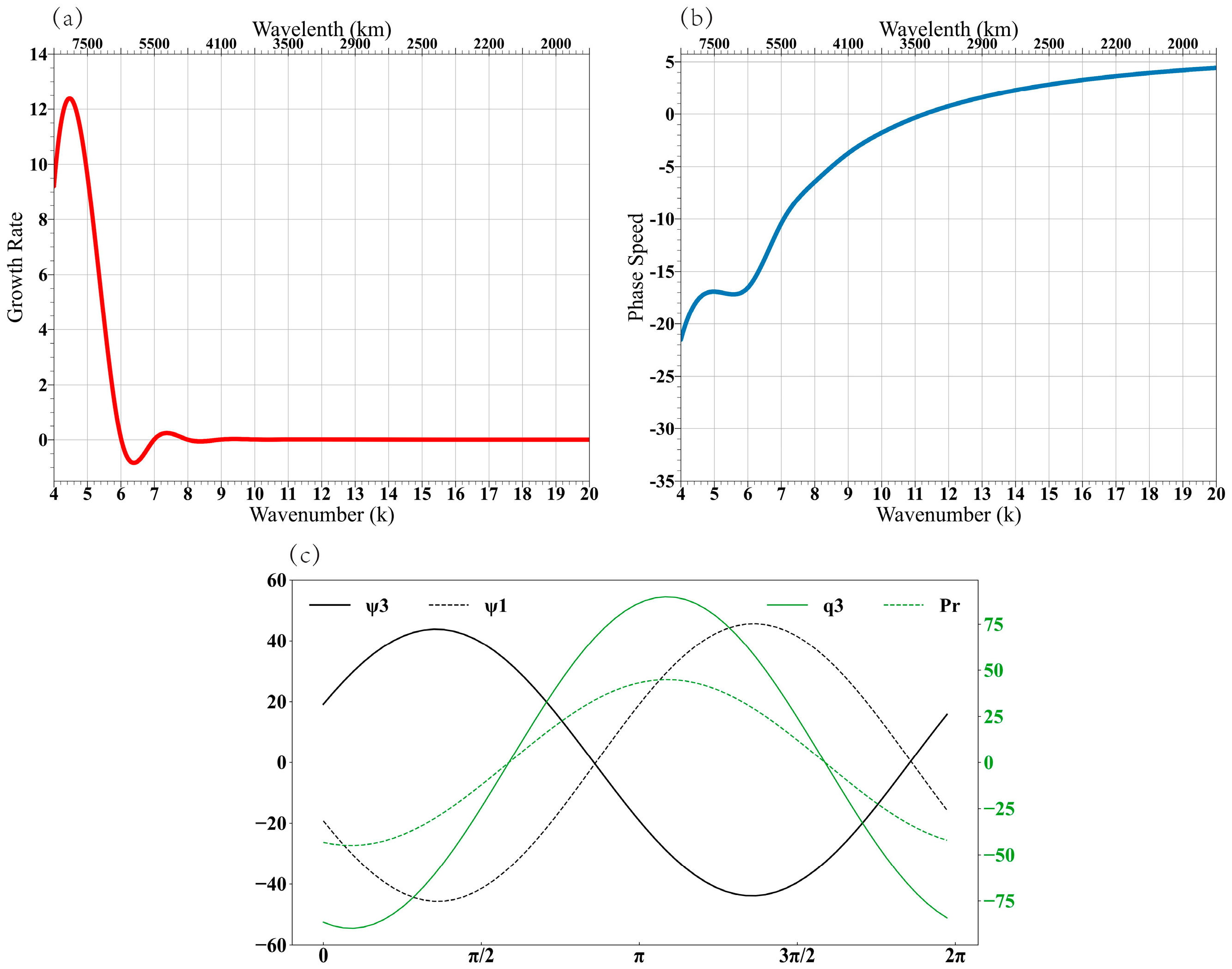
The pure effect of the MVI in affecting the growth rate may be assessed by removing the background vertical shear (simply by setting U1 = U3 = −3.5 m s−1). This sensitivity test result (Figure 10a) shows that in the absence of the background vertical shear, the growth rate decreases by 20% while the zonal wavelength of the most unstable mode increases to about 7500 km. This sensitivity experiment indicates that while the MVI is a dominant growth mechanism in the SASM and it explains about 80% of the total growth rate, the zonal scale selection depends on both the MVI and the BI. As shown later in Section 5, the vertical shear induced BI favors a shorter wavelength.
No vertical tilt is found in the absence of the background vertical shear (Figure 10c). The upper- and lower-tropospheric stream-function fields exhibit an out-of-phase relation, implying a first baroclinic mode vertical structure, triggered by the condensational heating in the mid troposphere.
The sensitivity experiment above also implies that the MVI can operate even in the absence of the low-level mean westerly. This contradicts the result of Adames (2021) [48], who emphasized the importance of the low-level mean westerly advection. Even in the presence of a low-level mean easterly, the MVI still operates, as long as Ekman-pumping-induced vertical moisture advection is in effect.
To sum up, the normal mode analysis of the current theoretical model indicates that in the presence of the moisture–convection–circulation feedback under a background easterly vertical shear, the model generates a very unstable mode that has a preferred synoptic-scale wavelength of about 4000 km, a westward phase speed of 6 m s−1, an eastward vertical tilt, and a westward shift of perturbation precipitation/moisture relative to the low-level cyclonic center. All of these features are in agreement with the observed counterparts. In the current framework, the MVI is a major mechanism determining the growth rate, while the vertical shear-induced BI plays an important role in modulating the preferred zonal scale of the perturbation.
5. Discussion
5.1. Does the Baroclinic Instability Operate in the Model?
Given the strong background easterly vertical shear, the classic BI may likely operate in the SASM. One way to reveal its effect in the current framework is to conduct a sensitivity experiment by setting the diabatic heating to zero.
Figure 11 shows the corresponding growth rate, phase speed, and zonal phase structures of the most unstable mode under the no-diabatic-heating scenario. In the absence of the heating, the QG dry dynamics are decoupled from the moistening process. The growth rate derived from this scenario reflects the pure effect of the classic BI.
Note that the growth rate decreases greatly (about 80%) in the absence of diabatic heating. This indicates that the vertical shear-induced BI is much weaker in the SASM than in the MVI. On the other hand, the BI alone favors a shorter zonal wavelength (about 3400 km). This implies that although its contribution to the growth rate is weak, the background vertical shear and associated BI still play an important role in modulating the perturbation zonal scale. In other words, the vertical shear effectively shortens the zonal wavelength of the developing disturbances.
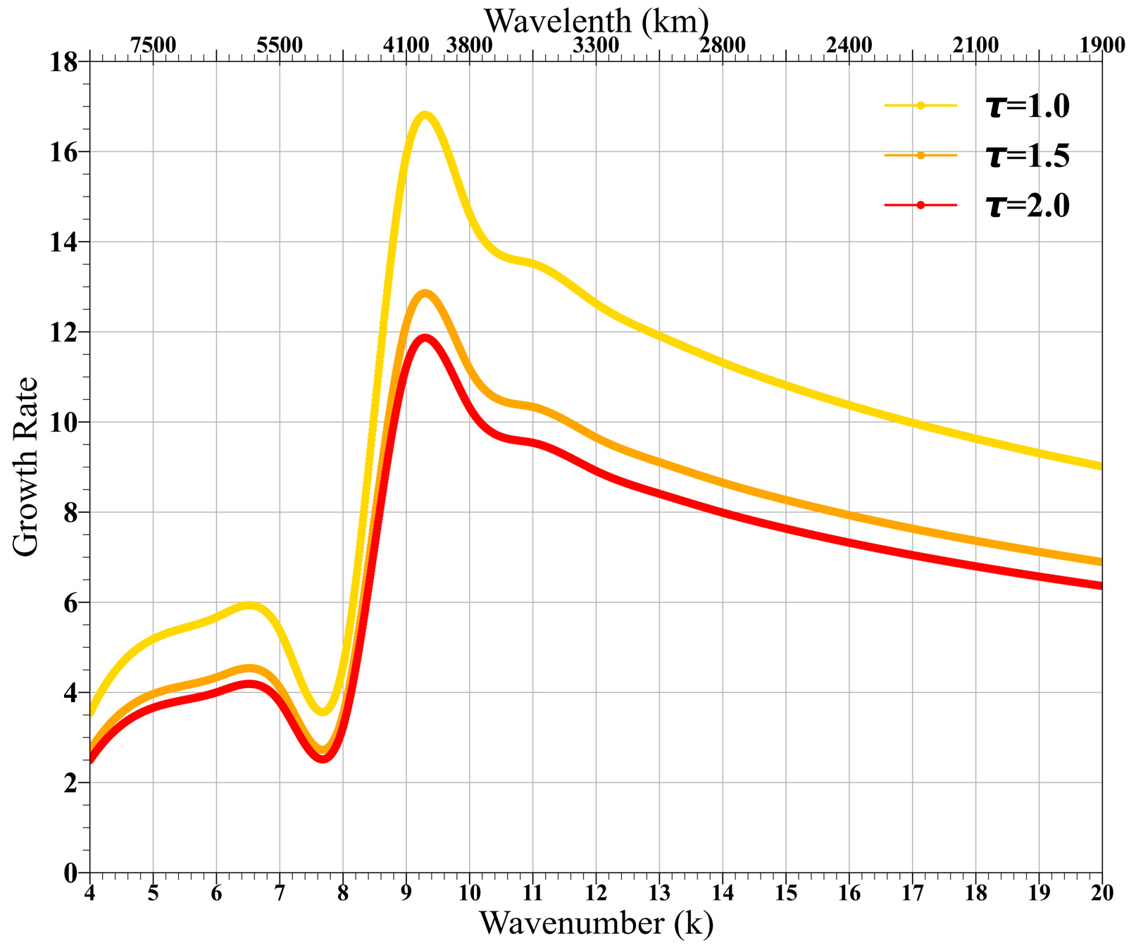
5.2. Dependence of the Growth Rate on Convective Adjustment Time
Equation (6) states that given the same amount of moisture, perturbation precipitation decreases with an increased convective adjustment time. This implies that a larger adjustment time should promote a weaker MVI. However, Adames (2021) [48] derived an opposite result. It is unclear why Adames (2021) obtained the controversial result. We speculate it might be attributed to simplifications and assumptions made during the derivation of the dispersion equation. In the current framework, the dispersion equation is derived directly from the three prognostic equations and solved with Newton’s iteration method (Yang and Li 2023) [54].
Figure 12 shows the sensitivity result of growth rates for given three different convective adjustment time values. As expected, the growth rate decreases as the adjustment time increases. Thus, the current MVI derives an opposite sensitivity of the growth rate to the adjustment time compared to that of Adames (2021) [48].
5.3. Issue of Observational Validation on the Role of the Baroclinic Instability in the SASM
Based on the observed composite of the vertical tilting structure of MDs, Cohen and Boos (2016) [44] proposed that the BI may not operate in the SASM region. Here, we argue that caution is needed in validating the BI theory against observations—one must focus on examining the vertical structure of a perturbation during its development phase. Note that selected MD cases in Cohen and Boos (2016) [44] were strong disturbances with a minimum surface pressure anomaly of 4-hPa. These MDs do not necessarily represent general synoptic disturbances in the region. Furthermore, the locations of the MDs in Cohen and Boos (2016) (see their Figure 1) are near the coast of India. Compared to the maximum synoptic variability center shown in Figure 3, most of the selected MDs are located either at or to the west of the maximum activity center. This implies that most of these depressions are either in their mature phase or during their decaying phase.
It is worth mentioning that despite the near coast tracks of the MDs, Cohen and Boos (2016) [44] looked at different lag days leading to the development of monsoon depressions. In contrast to Cohen and Boos (2016) [44], in the current observational analysis, we examined general synoptic-scale disturbances that have a period of less than 10 days. Our regression analysis with a much larger sample size shows that an easterly tilt does exist during the perturbation development phase to the east of the maximum variability center. This analysis result is consistent with a recent observational study by Luo et al. (2023) [55] (see their Figure 5). These results support the notion that the BI may somehow operate in the SASM.
6. Summary and Concluding Remarks
In this study, we re-examined the moisture–vortex instability (MVI) in a 2.5-layer model that considers Ekman-pumping-induced vertical moisture advection. To validate the model results with observations, an observational analysis of structure and evolution of dominant synoptic disturbances over the South Asian Monsoon region was carried out.
The observational analysis revealed that the south Asian monsoon is dominated by synoptic-scale disturbances that occupy 66% of total variabilities. The synoptic perturbations have a typical wavelength of 4000 km and a westward phase speed of 6 m s−1. A marked feature is the tight coupling of perturbation moisture and precipitation to circulation. The maximum moisture and precipitation anomalies are located to the west of the low-tropospheric cyclonic center, implying an important role of anomalous northerly in advecting higher mean moisture southward. An eastward tilt vertical structure is observed to the east of the maximum variability center during the disturbance development phase. This implies a possible role of the baroclinic instability in the region.
A 2.5-layer theoretical model was constructed to understand the origin of instability of the synoptic disturbances over the SASM region. This model is an extension of the classic QG two-level model of Phillips (1954) [37] by adding a prognostic lower-tropospheric moisture equation and an interactive PBL with Ekman-pumping-induced vertical moisture advection.
The normal mode analysis of the theoretical model shows that given realistic background vertical shear and meridional temperature/moisture gradients, the most unstable mode has a preferred zonal wavelength of 4000 km, a westward phase speed of 6 m s−1, and an eastward tilt vertical structure. These features are in agreement with the observations. In addition, the model also captures the observed zonal phase relationship among perturbation moisture, precipitation, and low-level cyclone, with maximum precipitation/ moisture anomaly centers located to the west of the anomalous cyclone.
Instability mechanisms through which perturbations grow in the current framework include both the MVI and the BI. As shown in Figure 8, a positive correlation between perturbation temperature and diabatic heating favors the increase of the perturbation APE. Meanwhile, a negative correlation between perturbation meridional wind and temperature in middle troposphere under a positive background meridional temperature gradient also favors the generation of the perturbation APE, providing an additional energy source.
Our sensitivity experiments reveal that the MVI plays a dominant role in controlling the growth rate, while the BI controls primarily the preferred zonal wavelength. This is demonstrated by removing the background vertical shear and the diabatic heating, respectively, in the model. In the absence of the vertical shear, only the MVI operates, and the growth rate under this special scenario attains 80% of that in the control experiment. The MVI preferred unstable wavelength, however, is much larger than the observed. In the absence of the diabatic heating, the model essentially returns to the classic QG model, and in such a system, only the BI operates. Our sensitivity result indicates that the BI alone favors a shorter wavelength. Thus, it is the combined effect of both the MVI and the BI that leads to an intermediate wavelength of 4000 km, agreeing with the observed.
It is worth mentioning that significant differences lie between the current model solution and that of Adames (2021) [48]. Firstly, the low-level mean westerly is no longer a necessary condition for the MVI to work. This is attributed to the effect of Ekman-pumping-induced vertical moisture advection. Secondly, the growth rate in the current model decreases as the convective adjustment time increases, which is opposite to Adames (2021) [48].
Although simple, the current theoretical framework is able to reproduce the observed preferred wavelength, phase speed, and horizontal and vertical structures. This suggests that both the MVI and the BI may operate in the SASM, and the combination of the two are capable of reproducing the observed characteristics of synoptic-scale disturbances over the SASM region. Given that moist barotropic instability may also operate in the SASM region, as demonstrated by Suhas and Boos (2023) [56], it is desirable to extend the current framework to include the meridional gradient of mean zonal flow, so that the relative roles of the MVI, moist barotropic and baroclinic instabilities may be assessed. One of such models is a three-dimensional anomaly general circulation model used by Li (2006) [49], who examined perturbation growth under either an idealized or a realistic three-dimentional background mean state. Such an effort will be carried out in the near future.
Author Contributions
H.C., T.L. and J.C. conceived the idea. H.C. conducted the data analyses and prepared Figures. H.C. wrote and reviewed the manuscript. All authors have read and agreed to the published version of the manuscript.
Funding
This research was supported by a NSFC grant 42088101.
Institutional Review Board Statement
Not applicable.
Informed Consent Statement
Not applicable.
Data Availability Statement
The daily interpolated OLR product is available from https://www.ncdc.noaa.gov/cdr/atmospheric (accessed on 1 September 2023). The ERA5 reanalysis data were downloaded from https://climate.copernicus.eu/climate–reanalysis (accessed on 1 September 2023).
Acknowledgments
Not applicable.
Conflicts of Interest
The authors declare no conflicts of interest.
References
- Wang, B.; Clemens, S.C.; Liu, P. Contrasting the Indian and East Asian monsoons: Implications on geologic timescales. Mar. Geol. 2003, 201, 5–21. [Google Scholar] [CrossRef]
- Yihui, D.; Chan, J.C. The East Asian summer monsoon: An overview. Meteorol. Atmos. Phys. 2005, 89, 117–142. [Google Scholar] [CrossRef]
- Ding, Y. The variability of the Asian summer monsoon. 気象集誌. 第 2 輯 2007, 85, 21–54. [Google Scholar] [CrossRef]
- Ding, Y. Seasonal march of the East-Asian summer monsoon. In East Asian Monsoon; World Scientific: Singapore, 2004; pp. 3–53. [Google Scholar]
- Qian, W.; Lee, D.K. Seasonal march of Asian summer monsoon. Int. J. Climatol. A J. R. Meteorol. Soc. 2000, 20, 1371–1386. [Google Scholar] [CrossRef]
- Turner, A.G.; Annamalai, H. Climate change and the South Asian summer monsoon. Nat. Clim. Chang. 2012, 2, 587–595. [Google Scholar] [CrossRef]
- Huang, R.; Sun, F. Impacts of the tropical western Pacific on the East Asian summer monsoon. J. Meteorol. Soc. Jpn. Ser. II 1992, 70, 243–256. [Google Scholar] [CrossRef]
- Zhang, L.; Liao, H.; Li, J. Impacts of Asian summer monsoon on seasonal and interannual variations of aerosols over eastern China. J. Geophys. Res. Atmos. 2010, 115, D00K05. [Google Scholar] [CrossRef]
- Zhao, C.; Wang, Y.; Yang, Q.; Fu, R.; Cunnold, D.; Choi, Y. Impact of East Asian summer monsoon on the air quality over China: View from space. J. Geophys. Res. Atmos. 2010, 115, D09301. [Google Scholar] [CrossRef]
- Saeed, F.; Hagemann, S.; Jacob, D. Impact of irrigation on the South Asian summer monsoon. Geophys. Res. Lett. 2009, 36. [Google Scholar] [CrossRef]
- Sun, Y.; Kutzbach, J.; An, Z.; Clemens, S.; Liu, Z.; Liu, W.; Liu, X.; Shi, Z.; Zheng, W.; Liang, L. Astronomical and glacial forcing of East Asian summer monsoon variability. Quat. Sci. Rev. 2015, 115, 132–142. [Google Scholar] [CrossRef]
- Li, T.; Wang, B. REVIEW A review on the western north Pacific monsoon: Synoptic-to-interannual variabilities. TAO Terr. Atmos. Ocean. Sci. 2005, 16, 285. [Google Scholar] [CrossRef] [PubMed]
- Li, T.; Hsu, P.-C.; Li, T.; Hsu, P.-C. Tropical cyclone formation. In Fundamentals of Tropical Climate Dynamics; Springer: Cham, Switzerland, 2018; pp. 107–147. [Google Scholar]
- Vogel, B.; Günther, G.; Müller, R.; Grooß, J.-U.; Hoor, P.; Krämer, M.; Müller, S.; Zahn, A.; Riese, M. Fast transport from Southeast Asia boundary layer sources to northern Europe: Rapid uplift in typhoons and eastward eddy shedding of the Asian monsoon anticyclone. Atmos. Chem. Phys. 2014, 14, 12745–12762. [Google Scholar] [CrossRef]
- Wang, D.; Zhang, Y.; Huang, A. Climatic features of the south-westerly low-level jet over southeast China and its association with precipitation over east China. Asia-Pac. J. Atmos. Sci. 2013, 49, 259–270. [Google Scholar] [CrossRef]
- Xavier, A.; Kottayil, A.; Mohanakumar, K.; Xavier, P.K. The role of monsoon low-level jet in modulating heavy rainfall events. Int. J. Climatol. 2018, 38, e569–e576. [Google Scholar] [CrossRef]
- Liu, H.; He, M.; Wang, B.; Zhang, Q. Advances in low-level jet research and future prospects. J. Meteorol. Res. 2014, 28, 57–75. [Google Scholar] [CrossRef]
- Li, X.; Ting, M.; You, Y.; Lee, D.E.; Westervelt, D.M.; Ming, Y. South Asian summer monsoon response to aerosol-forced sea surface temperatures. Geophys. Res. Lett. 2020, 47, e2019GL085329. [Google Scholar] [CrossRef]
- Zhang, Z.; Chan, J.C.; Ding, Y. Characteristics, evolution and mechanisms of the summer monsoon onset over Southeast Asia. Int. J. Climatol. A J. R. Meteorol. Soc. 2004, 24, 1461–1482. [Google Scholar] [CrossRef]
- Latif, M.; Syed, F.; Hannachi, A. Rainfall trends in the South Asian summer monsoon and its related large-scale dynamics with focus over Pakistan. Clim. Dyn. 2017, 48, 3565–3581. [Google Scholar] [CrossRef]
- Shukla, R.P. The dominant intraseasonal mode of intraseasonal South Asian summer monsoon. J. Geophys. Res. Atmos. 2014, 119, 635–651. [Google Scholar] [CrossRef]
- Ashfaq, M.; Shi, Y.; Tung, W.W.; Trapp, R.J.; Gao, X.; Pal, J.S.; Diffenbaugh, N.S. Suppression of south Asian summer monsoon precipitation in the 21st century. Geophys. Res. Lett. 2009, 36, L01704. [Google Scholar] [CrossRef]
- Huang, R.; Liu, Y.; Du, Z.; Chen, J.; Huangfu, J. Differences and links between the East Asian and South Asian summer monsoon systems: Characteristics and variability. Adv. Atmos. Sci. 2017, 34, 1204–1218. [Google Scholar] [CrossRef]
- Saeed, F.; Hagemann, S.; Jacob, D. A framework for the evaluation of the South Asian summer monsoon in a regional climate model applied to REMO. Int. J. Climatol. 2012, 32, 430–440. [Google Scholar] [CrossRef]
- Qian, W.; Zhu, Y. The comparison between summer monsoon components over East Asia and South Asia. J. Geosci. China 2002, 4, 17–32. [Google Scholar]
- Sikka, D.R. Synoptic and meso-scale weather disturbances over South Asia during the Southwest Summer monsoon season. In The Global Monsoon System: Research and Forecast; World Scientific: Singapore, 2011; pp. 183–204. [Google Scholar] [CrossRef]
- Nikumbh, A.C.; Chakraborty, A.; Bhat, G.; Frierson, D.M. Large-scale extreme rainfall-producing synoptic systems of the Indian summer monsoon. Geophys. Res. Lett. 2020, 47, e2020GL088403. [Google Scholar] [CrossRef]
- Huangfu, J.; Chen, W.; Lai, X.; Chen, D.; He, Z. Roles of synoptic-scale waves and intraseasonal oscillations in the onset of the South China Sea summer monsoon. Int. J. Climatol. 2022, 42, 2923–2934. [Google Scholar] [CrossRef]
- Wu, G.; Ren, S.; Xu, J.; Wang, D.; Bao, Q.; Liu, B.; Liu, Y. Impact of tropical cyclone development on the instability of South Asian High and the summer monsoon onset over Bay of Bengal. Clim. Dyn. 2013, 41, 2603–2616. [Google Scholar] [CrossRef]
- Huang, Q.; Guan, Y. Does the Asian monsoon modulate tropical cyclone activity over the South China Sea? Chin. J. Oceanol. Limnol. 2012, 30, 960–965. [Google Scholar] [CrossRef]
- Wang, X.; Zhou, W.; Li, C.; Wang, D. Effects of the East Asian summer monsoon on tropical cyclone genesis over the South China Sea on an interdecadal time scale. Adv. Atmos. Sci. 2012, 29, 249–262. [Google Scholar] [CrossRef]
- Chang, C.P.; Lei, Y.; Sui, C.H.; Lin, X.; Ren, F. Tropical cyclone and extreme rainfall trends in East Asian summer monsoon since mid-20th century. Geophys. Res. Lett. 2012, 39, L18702. [Google Scholar] [CrossRef]
- Kumar, V.; Krishnan, R. On the association between the Indian summer monsoon and the tropical cyclone activity over northwest Pacific. Curr. Sci. 2005, 88, 602–612. [Google Scholar]
- Loo, Y.Y.; Billa, L.; Singh, A. Effect of climate change on seasonal monsoon in Asia and its impact on the variability of monsoon rainfall in Southeast Asia. Geosci. Front. 2015, 6, 817–823. [Google Scholar] [CrossRef]
- Charney, J.G. The dynamics of long waves in a baroclinic westerly current. J. Atmos. Sci. 1947, 4, 136–162. [Google Scholar] [CrossRef]
- Eady, E.T. Long waves and cyclone waves. Tellus 1949, 1, 33–52. [Google Scholar] [CrossRef]
- Phillips, N.A. Energy transformations and meridional circulations associated with simple baroclinic waves in a two-level, quasi-geostrophic model. Tellus 1954, 6, 274–286. [Google Scholar]
- Pedlosky, J. An initial value problem in the theory of baroclinic instability. Tellus 1964, 16, 12–17. [Google Scholar] [CrossRef]
- Smagorinsky, J.; Manabe, S.; Holloway, J.L. Numerical results from a nine-level general circulation model of the atmosphere. Mon. Weather. Rev. 1965, 93, 727–768. [Google Scholar] [CrossRef]
- Hide, R.; Fowlis, W. Thermal convection in a rotating annulus of liquid: Effect of viscosity on the transition between axisymmetric and non-axisymmetric flow regimes. J. Atmos. Sci. 1965, 22, 541–558. [Google Scholar] [CrossRef]
- Holton, J.R. An introduction to dynamic meteorology. Am. J. Phys. 1973, 41, 752–754. [Google Scholar] [CrossRef]
- Shukla, J. CISK-barotropic-baroclinic instability and the growth of monsoon depressions. J. Atmos. Sci. 1978, 35, 495–508. [Google Scholar] [CrossRef]
- Mak, M. On moist quasi-geostrophic baroclinic instability in a general model. Sci. Sin. B 1983, 26, 850–864. [Google Scholar]
- Cohen, N.Y.; Boos, W.R. Perspectives on moist baroclinic instability: Implications for the growth of monsoon depressions. J. Atmos. Sci. 2016, 73, 1767–1788. [Google Scholar] [CrossRef]
- Kuo, H.L. Dynamic instability of two-dimensional nondivergent flow in a barotropic atmosphere. J. Atmos. Sci. 1949, 6, 105–122. [Google Scholar] [CrossRef]
- Diaz, M.; Boos, W.R. Monsoon depression amplification by moist barotropic instability in a vertically sheared environment. Q. J. R. Meteorol. Soc. 2019, 145, 2666–2684. [Google Scholar] [CrossRef]
- Adames, Á.F.; Ming, Y. Interactions between water vapor and potential vorticity in synoptic-scale monsoonal disturbances: Moisture vortex instability. J. Atmos. Sci. 2018, 75, 2083–2106. [Google Scholar] [CrossRef]
- Adames, Á.F. Interactions between water vapor, potential vorticity, and vertical wind shear in quasi-geostrophic motions: Implications for rotational tropical motion systems. J. Atmos. Sci. 2021, 78, 903–923. [Google Scholar] [CrossRef]
- Li, T. Origin of the summertime synoptic-scale wave train in the western North Pacific. J. Atmos. Sci. 2006, 63, 1093–1102. [Google Scholar] [CrossRef]
- Hsu, P.-c.; Li, T. Role of the boundary layer moisture asymmetry in causing the eastward propagation of the Madden–Julian oscillation. J. Clim. 2012, 25, 4914–4931. [Google Scholar] [CrossRef]
- Wang, B.; Li, T. A simple tropical atmosphere model of relevance to short-term climate variations. J. Atmos. Sci. 1993, 50, 260–284. [Google Scholar] [CrossRef]
- Liebmann, B.; Smith, C.A. Description of a complete (interpolated) outgoing longwave radiation dataset. Bull. Am. Meteorol. Soc. 1996, 77, 1275–1277. [Google Scholar]
- Hersbach, H. Global reanalysis: Goodbye ERA-Interim, hello ERA5. ECMWF Newsl. 2019, 159, 17. [Google Scholar]
- Yang, G.; Li, T. Moist Baroclinic Instability along the Subtropical Mei-Yu Front. J. Clim. 2023, 36, 805–822. [Google Scholar] [CrossRef]
- Luo, H.; Adames Corraliza, Á.F.; Rood, R.B. Barotropic and Moisture–Vortex Growth of Monsoon Low Pressure Systems. J. Atmos. Sci. 2023, 80, 2823–2836. [Google Scholar] [CrossRef]
- Suhas, D.; Boos, W.R. Monsoon depression amplification by horizontal shear and humidity gradients: A shallow water perspective. J. Atmos. Sci. 2023, 80, 633–647. [Google Scholar] [CrossRef]
Figure 1.
The climatological JJA mean patterns of (a) OLR (shading; W m−2) and 850-hPa wind (vector; m s−1) fields; (b) vertical wind shear (shading; m s−1) obtained by subtracting 850-hPa zonal wind from 200-hPa zonal wind; (c) 925-hPa specific humidity (shading; g kg−1); and (d) the temperature averaged from 850-hPa to 200-hPa (shading; K) and from 500-hPa to 200-hPa (contour; K).

Figure 2.
(a) The standard deviation of daily OLR anomalies (shading; W m−2). The blue, brown, and green boxes denote three significant OLR variability centers. (b–d) Power spectra of daily OLR anomalies averaged over the three boxes: 14–18° N, 67–71° E (blue box), 14–18° N, 83–87° E (brown box), and 14–18° N, 113–117° E (green box), respectively. The dashed red curves denote the 95% confidence level.

Figure 3.
(a) The standard deviation of synoptic-scale OLR (shading; W m−2) field; and (b) the standard deviation of synoptic-scale (orange bar) and total (green bar) OLR (unit: W m−2) fields averaged over 14–18° N, 83–87° E (i.e., the black box shown in Figure 3a).
Figure 3.
(a) The standard deviation of synoptic-scale OLR (shading; W m−2) field; and (b) the standard deviation of synoptic-scale (orange bar) and total (green bar) OLR (unit: W m−2) fields averaged over 14–18° N, 83–87° E (i.e., the black box shown in Figure 3a).

Figure 4.
Horizontal patterns of (a–c) regressed synoptic-scale OLR field (shading; W m−2), 850-hPa wind (vector; m s−1), and 850-hPa geopotential height (contour; m2 s−2) fields from day −2 to day 0. (d–f) As in (a–c), but for synoptic-scale 700-hPa specific humidity (shading; g kg−1), 850-hPa wind (vector; m s−1) and 850-hPa geopotential height (contour; m2 s−2) fields from day −2 to day 0. The yellow dots represent the maximum convective centers. Magenta and blue arrows show the westward phase propagation and a half-zonal wavelength of the synoptic-scale disturbances, respectively.

Figure 5.
(a–c) Zonal-vertical cross-sections of regressed synoptic-scale specific humidity (shading; g kg−1) and geopotential height (contour; m2 s−2) fields averaged from 16–18° N from day −2 to day 0. The selection of this latitude zone is to take into consideration both the specific humidity and geopotential height center locations. Positive contours are represented by solid lines and negative contours are dashed.

Figure 6.
Schematic for the vertical levels of the 2.5-layer moist baroclinic model.

Figure 7.
(a) Growth rate (unit: 10−6 s−1); and (b) phase speed (unit: m s−1) as a function of zonal wavenumber (k) derived from the current theoretical model.
Figure 7.
(a) Growth rate (unit: 10−6 s−1); and (b) phase speed (unit: m s−1) as a function of zonal wavenumber (k) derived from the current theoretical model.

Figure 8.
Zonal phase relations among barotropic stream-function (unit: 107 m2 s−1), baroclinic stream-function (unit: 107 m2 s−1) and lower-tropospheric specific humidity (unit: g kg−1) for the most unstable mode in the moist baroclinic model.
Figure 8.
Zonal phase relations among barotropic stream-function (unit: 107 m2 s−1), baroclinic stream-function (unit: 107 m2 s−1) and lower-tropospheric specific humidity (unit: g kg−1) for the most unstable mode in the moist baroclinic model.

Figure 9.
(a) Zonal phase relations among lower-tropospheric stream-function (unit: 107 m2 s−1), upper-tropospheric stream-function (unit: 107 m2 s−1), lower-tropospheric specific humidity (unit: g kg−1) and precipitation (unit: mm day−1) derived from the theoretical model. (b) Zonal phase relations of observed synoptic-scale geopotential height fields at 850 hPa and 500 hPa (unit: m2 s−2), specific humidity at 700 hPa (: unit: 10−1 g kg−1) and -OLR (shading; 101 W m−2) derived based on the composite of day −1 and day 0 in Figure 5, with the low-level low-pressure center as a reference longitude.

Figure 10.
(a) Growth rate (unit: 10−6 s−1); and (b) phase speed (unit: m s−1) as a function of zonal wavenumber (k) derived from the current model in the absence of background vertical shear with U1 = U3 = −3.5 m s−1; (c) corresponding zonal phase relations among lower and upper stream-function and (unit: 107 m2 s−1), lower-tropospheric specific humidity (unit: g kg−1) and (unit: mm day−1) for the most unstable mode in the absence of background vertical shear with U1 = U3 = −3.5 m s−1.

Figure 11.
(a) Growth rate (unit: 10−6 s−1); and (b) phase speed (unit: m s−1) as a function of zonal wavenumber (k) derived from the analytical model in the absence of the diabatic heating; (c) Zonal phase relations among lower and upper tropospheric stream-function and (unit: 107 m2 s−1) and lower-tropospheric specific humidity (unit: g kg−1) and (unit: mm day−1) for the most unstable mode in the absence of the diabatic heating.

Figure 12.
Growth rate (unit: 10−6 s−1) as a function of zonal wavenumber (k) calculated from the model with three convective adjustment time values, 1.0, 1.5, and 2.0 days.
Figure 12.
Growth rate (unit: 10−6 s−1) as a function of zonal wavenumber (k) calculated from the model with three convective adjustment time values, 1.0, 1.5, and 2.0 days.


Table 1.
Controlled parameter values used in the 2.5-layer model.
| Angular speed of rotation of the Earth | |
| Radius of the Earth | |
| Reference latitude | |
| Gas constant for dry air | |
| Specific heat of dry air at constant pressure | |
| Ratio of gas constant to specific heat at constant pressure | |
| Latent heat of vaporization | |
| Density scale height | |
| Pressure interval between level 1 and 3 | |
| Mean zonal velocity at levels 1 | |
| Mean zonal velocity at levels 3 | |
| Mean meridional specific humidity gradient | |
| Mean vertical specific humidity gradient | |
| Eddy viscosity coefficient | |
| Ekman friction coefficient | |
| Static stability parameter | |
| Convective adjustment time |
Disclaimer/Publisher’s Note: The statements, opinions and data contained in all publications are solely those of the individual author(s) and contributor(s) and not of MDPI and/or the editor(s). MDPI and/or the editor(s) disclaim responsibility for any injury to people or property resulting from any ideas, methods, instructions or products referred to in the content. |
© 2024 by the authors. Licensee MDPI, Basel, Switzerland. This article is an open access article distributed under the terms and conditions of the Creative Commons Attribution (CC BY) license (https://creativecommons.org/licenses/by/4.0/).
Share and Cite
MDPI and ACS Style
Chen, H.; Li, T.; Cui, J. The Reexamination of the Moisture–Vortex and Baroclinic Instabilities in the South Asian Monsoon. Atmosphere 2024, 15, 147. https://doi.org/10.3390/atmos15020147
AMA Style
Chen H, Li T, Cui J. The Reexamination of the Moisture–Vortex and Baroclinic Instabilities in the South Asian Monsoon. Atmosphere. 2024; 15(2):147. https://doi.org/10.3390/atmos15020147
Chicago/Turabian StyleChen, Hongyu, Tim Li, and Jing Cui. 2024. "The Reexamination of the Moisture–Vortex and Baroclinic Instabilities in the South Asian Monsoon" Atmosphere 15, no. 2: 147. https://doi.org/10.3390/atmos15020147
Note that from the first issue of 2016, this journal uses article numbers instead of page numbers. See further details here.