Novel Intelligent Methods for Channel Path Classification and Model Determination Based on Blind Source Signals

Abstract

In this paper, the urban signal propagation characteristics based on the location of blind sources are investigated. To address the issue of blind electromagnetic radiation sources in complex urban environments, intelligent methods for propagation channel path classification, and model determination are brought forth based on field test data. The intelligent classification method distinguishes between the Line-of-Sight (LoS) path channel and a direct path, the LoS multipath channel with a direct path and other multiple paths, and the Non-Line-of-Sight (NLoS) multipath channel without a direct path from the source to the test point. The modeling aspect determines the model type to which the received signal belongs based on the statistical model derived from the tested data of a specific source. A validation measurement system was constructed for the FM broadcasting band, and validation campaigns were conducted in the city of Wuhan. The process and analysis of the data using this method demonstrate the accurate distinction of the different propagation path channels and models and involve the construction of a statistical model for the FM band in Wuhan’s urban area.

1. Introduction

The channel path classification and the model determination of electromagnetic wave propagation play a crucial role in wireless system applications and relevant research. In the field of radio wave propagation research, it is essential to develop classification methods for propagation channel paths and distinguish between different propagation modeling methods. This will help in obtaining research results that can explain the propagation mechanism and phenomena, guide the design of wireless systems, and facilitate the development of new wireless applications. The development of new wireless mobile communication technologies like 5G, 5G-beyond, and 6G necessitates accurate information on wireless propagation channels, timely automated classification of their propagation channel paths, and the determination of propagation models to ensure the proper functioning of the systems. Traditional research on radio wave propagation adopts a point-to-point approach to construct dedicated propagation paths for analyzing channel path types and establishing propagation models. This approach forms the fundamental method and research outcomes for signal observation and data processing in subsequent studies [1]. However, these methods and results have not been able to meet the demands of mobile applications and the rapid development of new wireless technologies, particularly in the emerging field of integrated smart wireless communication and sensing. Specifically, real-time estimation of channel path types and propagation models is necessary. The advancement of signal-sensing technology in mobile networks has enabled the development of novel methods for classifying and modeling propagation channels. Support Vector Regression, matrix dimensionality reduction techniques, artificial neural networks, and Vehicle-to-Vehicle channel measurements are contributing to the continuous improvement of channel modeling and analysis methods [2,3,4,5].

In various channel research scenarios, self-constructed transmitters, omnidirectional antennas, antenna arrays, receivers, and other RF equipment are mostly used [6,7,8]. In the analysis of propagation channels involving propagation mechanisms, path classification, and propagation modeling, path classification is influenced by various factors in the system’s geo-topological structure, in addition to the system equipment. In propagation modeling, the empirical model of radio wave propagation in various environments (also known as the empirical statistical model) is based on extensive measured data [9,10,11], and the deterministic model based on physical principles is commonly used [12,13,14]. These two models can be combined to develop a semi-empirical model. This often poses challenges in terms of facility establishment, test duration, facility maintenance, personnel security, and applicability to different scenarios. The above problems bring some inconvenience to channel modeling. Nowadays, it is possible to collect signal observation data in real time and in different locations within the application area. These data can be utilized to develop novel methods and techniques for classifying propagation channel paths and determining propagation models based on wireless mobile network signals [15,16,17]. However, the challenge lies in the blind source of the observed signal whose information, such as location and radiation characteristics, is unknown. By addressing the blind source problem of the radiated source information, new methods for classifying propagation channels and modeling propagation should be developed. The blind source problem was initially introduced by Jeanny Herault and Christian Jutten in the field of signal separation [18]. Exploring the acquisition of the blind sources of wireless signal radiation and their utilization for propagation between the source and the receiving site remains an area that requires further investigation [19,20,21]. Therefore, in order to simplify the scenarios of channel research, meet the new scenarios of future radio applications, and explore the possibility of blind source channel modeling, this paper puts forward a new method.

Based on this, novel intelligent methods for channel path classification and model determination based on blind source signals are investigated. The specific sections are as follows: Section 2 presents the theory for propagation channel path classification and model determination. Section 3 presents the localization method, the channel path classification method, and the verification measurement system established to obtain the required data. Section 4 illustrates the results of the analysis of the FM measurements at 92.7 MHz and 95.6 MHz, which validates the method proposed in this paper. Section 5 gives conclusions and prospects.

2. Propagation Channel Paths and Models

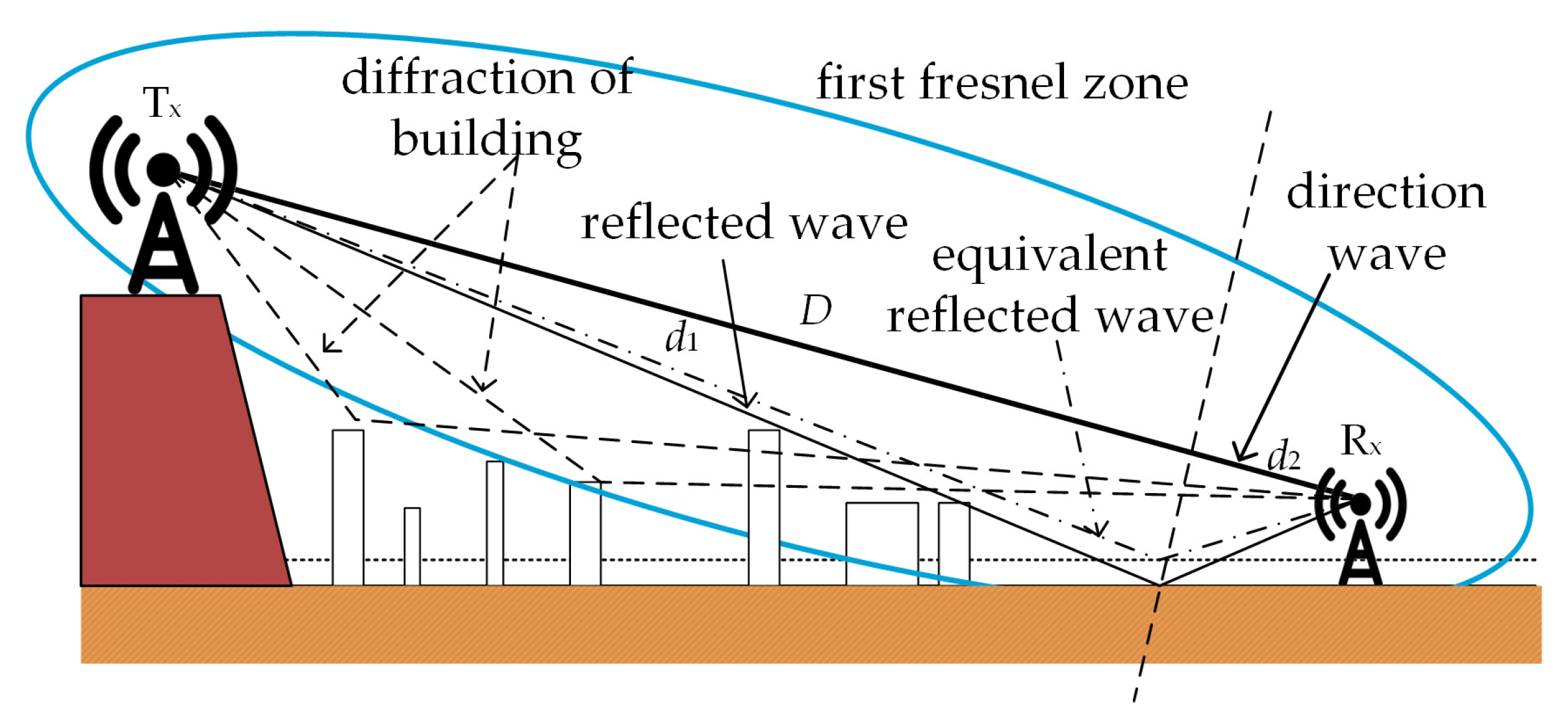
2.1. Propagation Channel Paths

In real scenarios, the propagation environment can be complex. Changes in the environment between the receiving and transmitting sites can result in different propagation models. Factors such as varying building heights and terrain can lead to multiple propagation paths, including direct wave rays (the direct path) and reflected wave rays, diffraction wave rays, and scattered rays (the non-direct path), forming different types of path channels. The actual received signal is a combination of signals from the various paths at the receiving site. Figure 1 illustrates a common wireless system setup in a city, where the transmitter (Tx) is typically located at a high point, while the mobile user (Rx) is closer to the ground. If the object between the user and the transmitter is low enough, the wave can propagate straight through, forming a direct wave path channel. However, if the object blocks the wave, it creates a non-direct wave path channel. For example, the top of a building, as shown in Figure 1, can generate a diffraction wave path channel, while flatter ground can produce a reflected path wave.

According to the theory of radio wave propagation, the direct and non-direct path channels are influenced by factors such as the frequency (wavelength) of the wireless signal, the size of the object, and the antenna configuration of the transceiver. The resulting measurement signal is a combination of these contributions, which can lead to coherent enhancement or attenuation in different regions. By utilizing the Fresnel zones, it is possible to effectively classify between different channel paths.

The Fresnel zone is an elliptical space with two focal points representing the transmitting and receiving antennas. While there are an infinite number of Fresnel zones, the first Fresnel zone (the blue ellipse in Figure 1) is typically sufficient. The radius of the first Fresnel zone is defined as follows:

$$R=\sqrt{\frac{\lambda d_1{d}_2}{D}}$$

(1)

where D is the distance from the transmitting point to the receiving point in m, d₁ is the distance between the intersection point, which is the vertical line through the reflection point and D and the transmitting point in m, d₂ is the distance between the intersection point which is the vertical line through the reflection point and D and the receiving point in m, $\lambda$ is the wavelength of the transmitting signal in m.

The channel classification in this paper categorizes the channels between the transmitting site and the receiving sites into three groups based on the paths observed in the first Fresnel zone. The propagation channel is a Line-of-sight (LoS) path channel if there is only a direct path between the transmitter and receiver. A channel that consists of the direct and non-direct path is referred to as a multi-Line-of-sight (multi-LoS) channel, while channels without a LoS path but with multipath waves are called Non-Line-of-Sight (NLoS) multipath channels.

2.2. Statistical Model of Wave Propagation

This is the basic approach for large-scale channel modeling, encompassing wireless signal networks across a range of frequency bands, including traditional bands, modern Sub-6 GHz bands, and even higher frequency bands like mm-waves that are being developed for mobile communications. However, modeling for different frequency bands, such as 3G, 4G, 5G, and potentially 6G, requires certain adjustments based on the application characteristics and physical properties of the bands [22,23,24,25]. In this paper, the VHF frequency band, which has numerous applications in the modern communication field, is selected. For the VHF or near-VHF band, there are two established models, namely the Okumura–Hata model and the Egli model.

2.2.1. Basic Statistical Model

These models are statistical models that have been derived from empirical formulas based on observed signals and propagation scenarios. The propagation loss of a wireless signal at a specific frequency is determined by the ground distance d. To simplify the fitting process, the multiplicative factors related to frequency and distance are kept constant. In summary, the models can be summarized as follows:

$$L_{new}=A+M\log (d)+M\log (f)+\chi$$

(2)

where A is the constant of the corresponding fitting function of the model large-scale propagation, M is the constant corresponding to the inverse of the square of the distance and frequency in the free space, and $\chi$ is the fading caused by multipaths and other factors. This describes the channel characteristics in a certain space or time, and it contains the multipath delay and doppler shift brought about by the small-scale fading. The information about small-scale fading can be obtained by studying its distribution over distance in detail [26]. Equation (2) can be used to fit the measured dataset, allowing the construction of an average propagation model. This model captures the variations in the propagation environment as signals travel from the transmitting site to different receiving sites.

2.2.2. Okumura–Hata Model

Hata studied and analyzed Okumura’s prediction curves and obtained an empirical formula for easy computation [27], which is applicable to the 150 MHz–1500 MHz, with the requirement of 1–20 km for the ground distance between the receiving and transmitting site.The effective height of the transmitting antenna is 30–200 m, as the effective height of the receiving antenna is 1–10 m.

The model formula is as follows:

$$L_U=69.55+26.16\log (f)-13.82\log (h_B)+[44.9-6.55\log (h_B)]\log (d)-\alpha (h_M)$$

(3)

In Equation (3), L_U is the propagation loss in the urban area in dB, h_B is the height of the transmitting antenna in m, f is the transmitting frequency in MHz, d is the ground distance between the transmitting and receiving site in km, and α(h_M) is the factor related to the height and frequency of the receiving antenna. In the small and medium cities, α(h_M) is as follows:

$$\alpha (h_M)=[1.1\log (f)-0.7]h_M-[1.56\log (f)-0.8]$$

(4)

In the large city, α(h_M) is as follows:

$$\alpha (h_M)=\{\begin{array}{l}8.29{[\log (1.54h_M)]}^2-1.1,150\mathrm{MHz}\le f\le 200\mathrm{MHz}\\ 3.2{[\log (11.75h_M)]}^2-4.97, 200\mathrm{MHz}\le f\le 1500\mathrm{MHz}\end{array}$$

(5)

where h_M is the height of the receiving antenna. In the FM band, which is considered in this paper for modeling, the wavelength falls within the range of 2.7 to 3.4 m. The Okumura–Hata model, which has a minimum wavelength requirement of about 3 m, can still be applied in this case. Although there may be a systematic error due to the limited applicable range of the model, the error is expected to be consistent in the same direction. Hence, the Okumura–Hata model can be used for modeling in the FM band.

2.2.3. Egli Model

Egli proposed this model for predicting the propagation of radio waves over irregular terrain in the frequency band 40–1000 MHz [28]. After post-optimization, the formula of the model is as follows:

$$L_U=20\log (f)+40\log (d)-20\log (h_B)-K_h+\{\begin{array}{l}76.3-10\log (h_M),h_M\le 10\\ 85.9-20\log (h_M),h_M>10\end{array}$$

(6)

In the above equation, L_U, f, d, h_M, and h_B have the same meaning as the Okumura–Hata model. When d is less than 30 km, the frequency range is 40–450 MHz, and there are no specific requirements for the transceiver’s height. K_h is the terrain correction factor in dB, which is used to reflect the effect of terrain on propagation loss. The frequency band involved in this paper is the FM band, so it is determined by the following equation:

$$K_h=1.667-0.1094\Delta h$$

(7)

where Δh is the undulation height of the terrain, which in this paper is 23.3 m in the campaign area of the city. The test scenario in this paper satisfies the requirements of the above two models.

2.3. Deterministic Model of Wave Propagation

Deterministic models determine the propagation loss through numerical calculation based on electromagnetic wave propagation theory, and a representative model is the one-way standard atmosphere parabolic equation (hereafter called standard atmosphere).

One-way Standard Atmospheric Parabolic Equation

The formula of radio wave propagation in the right-angle coordinate system is as follows:

$$\left[\frac{{\partial }^2}{\partial x^2}+2ik\frac{\partial }{\partial x}+\frac{{\partial }^2}{\partial z^2}+k^2(n^2-1)\right]u(x,z)=0$$

(8)

If the atmospheric refraction factor n does not change with distance x, the above equation can be decomposed as follows:

$$\left[\frac{\partial }{\partial x}+ik(1-Q)\right]\left[\frac{\partial }{\partial x}+ik(1+Q)\right]u(x,z)=0$$

(9)

where $Q=\sqrt{\frac{1}{k^2}\frac{{\partial }^2}{\partial z^2}+n^2(x,z)}$, considering the forward propagation only, it can be further separated as follows:

$$\frac{\partial u}{\partial x}=-ik(1-Q)u$$

(10)

The propagation loss is obtained from Equation (10) in [29].

3. The Intelligent Methods and Data Acquisition System

3.1. The Method of Positioning the Blind Source

The method described in the paper utilizes the particle swarm algorithm as its main component, with the genetic algorithm embedded within it [30]. This combination effectively combines the strengths of global search and local search, resulting in improved search performance [31]. To prevent the algorithm from getting trapped in local optima, the inertia weights are set to decrease linearly. This ensures that the algorithm searches rapidly in the initial stages while producing more accurate results in the later stages [32]. The fusion algorithm in this paper employs the parameters shown in

Table 1. Parameters of fusion intelligence algorithm.

Parameter	Value
Maximum number of iterations	100
Population size	80
Individual learning factor	1.4
Social learning factor	1.4
Maximum inertia factor	0.9
Minimum inertia factor	0.4
Maximum exchange rate	0.2
Minimum exchange rate	0
Maximum mutation rate	0.2
Minimum mutation rate	0

. The number of iterations and population size are both correlated with the search space and search time. The typical range of population size is from 10 to 100. A larger population size allows for more exploration but may increase computation time. The inertia weight controls the balance between exploration and exploitation, with typical values ranging from 0.4 to 0.9. A higher value promotes exploration, while a lower value promotes exploitation. The individual learning factor and social learning factor are parameters that control the influence of the particle’s personal best position and the global best position, respectively; typical values range from 1 to 2. A higher cognitive weight emphasizes personal experience, while a higher social weight emphasizes the influence of the swarm. The exchange rate represents the probability of crossover occurring between two individuals during reproduction, with typical values ranging from 0.2 to 0.9 [33,34]. A higher crossover rate promotes exploration and genetic diversity. The mutation rate represents the probability of a gene mutation occurring during reproduction, with typical values ranging from 0.01 to 0.2. A higher mutation rate allows for more exploration and prevents premature convergence [35]. The parameter values in Table 1 are chosen considering the search accuracy and search time.

During the search, each particle carries three parameters of information, namely, longitude, latitude, and the EIRP (equivalent isotropic radiant power) of the radiation source. The fitness function is defined as follows:

$$f_{fitness}=\sqrt{{(P_{real}-P_{predict})}^2}$$

(11)

where P_real is the power of the signal received in dBm, and P_predict is the predicted received power in dBm. P_predict is defined as follows:

$$P_{predict}=EIRP-L$$

(12)

where L is the propagation loss in the free space in dB; its formula is expressed as follows:

$$L=32.4+20\log (d)+20\log (f)$$

(13)

where d and f are the same meaning mentioned in Section 2. After the iteration stops, the information carried by the particle with the smallest fitness is the desired information. The flowchart of the algorithm is shown in Figure 2:

The final position results are shown in the

Table 2. Result of fusion intelligence algorithm.

Latitude/Degree	Longitude/Degree	EIRP/dBm
114.27	30.55	91.27

:

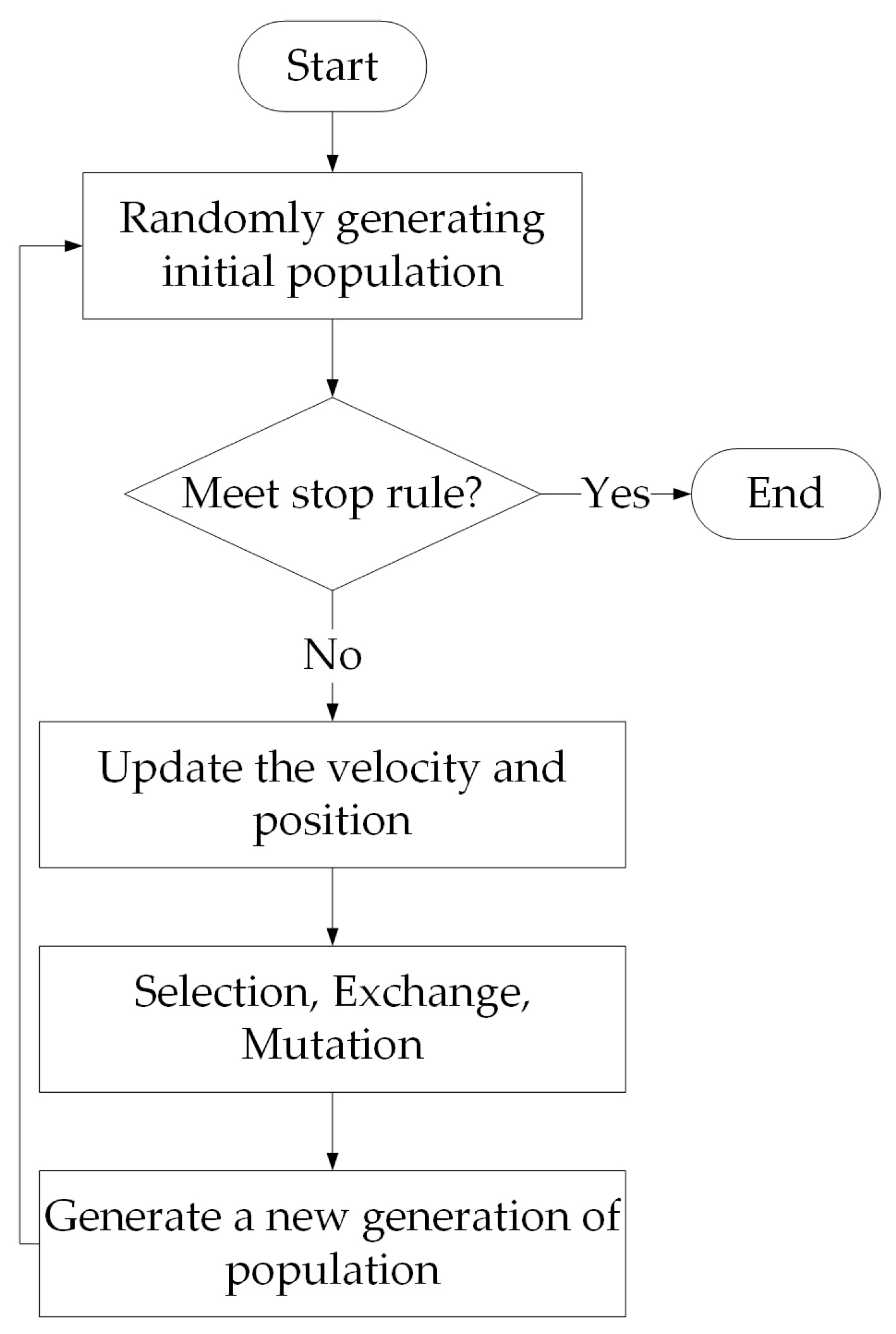
3.2. Methods of Channel and Model Type Differentiation

It can be seen that the max Fresnel radius is $\frac{\sqrt{\lambda D}}{2}$ in Equation (1), when d₁ = d₂, and if there are buildings or vegetation in this area, it will have a greater impact on the signal strength of the receiving site. On the basis of confirming the location of the blind source, determining whether there are buildings in the path between each receiving site and the source in the Fresnel zone to ensure the presence of NLoS channels and LoS channels. The method of channel classifying is as follows:

(1)

Obtain all the paths, the first Fresnel zone of the receiving point, and the source transmitting point.

(2)

If there is a blocker, such as a building, on this path, the channel is an NLoS channel (without a direct path).

(3)

If there is no blocker in the first Fresnel zone, it is a LoS channel (only the direct path).

(4)

If there is a blocker in the first Fresnel zone, but it is not blocking the direct link between Tx and Rx, then it is a multi-LoS channel (the direct and non-direct paths).

Based on the DBSCAN (Density-Based Spatial Clustering of Application with Noise) clustering method [36], the points that are more concentrated in the data can be considered as the same model, and the advantage of density-based clustering is that there is no need to specify the number of clusters. They can be considered as different propagation models when cluster 1 and cluster 2 are 3 dB away from each other. Based on this, different propagation models can be determined by solving the number of clusters in a segment of the spatial domain. The method of model determination is as follows:

(1)

Obtain a single standard parabolic equation, Egli, and Okumura–Hata model’s data.

(2)

The three models are used as the center to extend the domain radius outward, and the data within the radius of the connected neighborhood is a class of models.

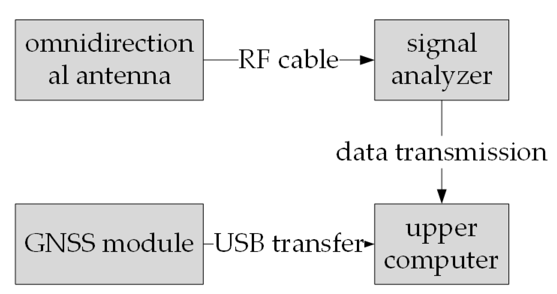
3.3. Data Acquisition System

To analyze the channel characteristics, the location of the transmitting source is required. In order to obtain these data, a system for monitoring radio signals from existing artificial sources is designed using intelligent data acquisition techniques. This system is capable of receiving a large number of radio signals from the study area through mobile measurements. The received data includes information such as time, longitude, latitude, altitude, and received power of the signals. The hardware system architecture for this monitoring system is depicted in the block diagram shown in Figure 3. The external shortwave FM antenna is connected to a signal analyzer, which captures the data within the specified bandwidth. These data are then transmitted to the host computer for further calculation and display. Additionally, a Global Navigation Satellite System (GNSS) module is directly connected to the host computer to provide real-time latitude, longitude, and altitude information. The host computer is responsible for measurement control, information display, and data acquisition.

Based on the data collected by the hardware system, intelligent algorithms can be used to obtain the location information of the transmitting source.

4. Validation Results and Analysis

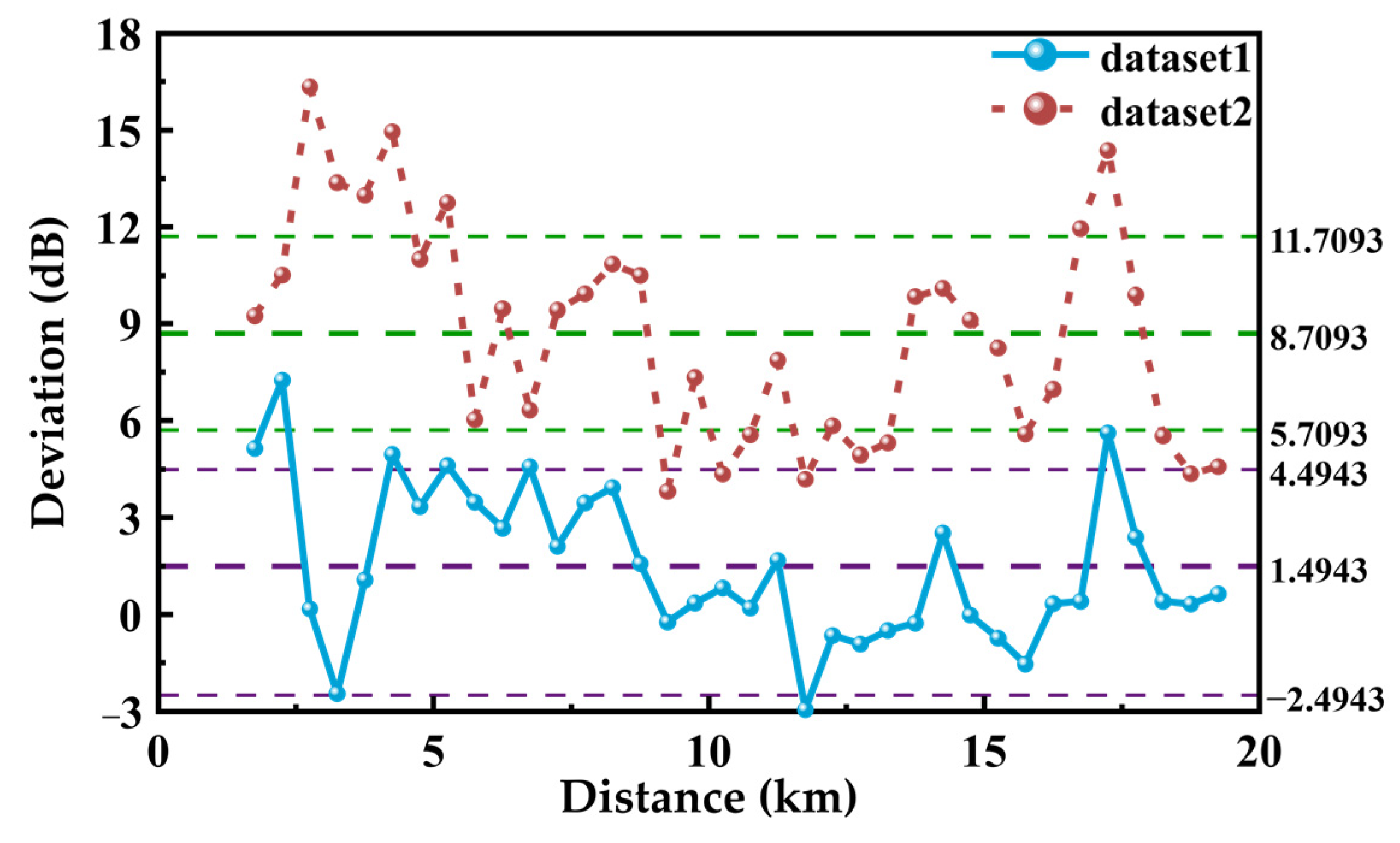
4.1. Measurement Data and Processing

The dataset used in this study was obtained from on-board mobile measurements conducted in Wuhan. Specifically, data from two FM radio station signals were selected, one at 92.7 MHz and the other at 95.6 MHz. These measurements were taken on two different dates, 5 November 2022 and 8 April 2023. The dataset consists of a total of 14,688 data points, with 7580 data points for dataset 1 and 7108 data points for dataset 2.

Due to the existence of small-scale fading, the signal power produces a change of 30–40 dB over spatial distances of the wavelength order of magnitude, which means that signal amplitude will change by a factor of 1000–10,000 when varying over short distances, and post-processing of the collected data is required for the classification of the large-scale channel models. In order to weaken the effects of small-local fading, the processing is based on the wavelength of the acquired signal, and the local received power needs to be in the range of 20–40$\lambda$ [37]. In this paper, the wavelength of the acquired signal is approximately 3.0 m. Additionally, the average speed of the experimental vehicle during the measurements is 44.9 km/h. Based on these parameters, the distance covered by the vehicle in 6 s is approximately 72 m. Since this distance is greater than 20 times the wavelength, an average is performed using six data points. During the averaging process, the position data of the third data point is used. After the averaging and processing steps, the number of data points in Dataset 1 is reduced to 1263, while Dataset 2 is reduced to 1184.

4.2. Channel Path Classification

Figure 4a shows the regional distribution of LoS path channels (LoS), LoS multipath channels (multi-LoS), and NLoS multipath channels (NLoS) in campaign 1. Figure 4b shows the regional distribution of LoS channels, multi-LoS channels, and NLoS channels in campaign 2 (The origin point is at the transmitting point).

Table 3. Percentage of each channel type.

Campaign Number	Channel Type	Percentage	Number
1	LoS	47.19%	596
	NLoS	44.26%	559
	Multi-LoS	5.38%	68
2	LoS	46.28%	548
	NLoS	48.82%	578
	Multi-LoS	2.45%	29

shows the number of LoS channels, multi-LoS channels, and NLoS channels on Path 1 and Path 2. The results calculated by the method proposed in Section 3 are shown in Figure 5 and Table 3.

Multi-LoS channels have the lowest percentage due to the vast majority of buildings and vegetation present in the city on the propagation path, making an NLoS channel when it is shaded by a building and a LoS channel when it is in the unshaded building gap or street. To generate a multi-LoS channel, it is necessary to have, firstly, an LoS channel. There must be a reflecting point that can reach the receiving site, and there are very few data that fulfill both conditions, so the multi-LoS channels produce the least. The results in Table 3 have an average of 93.28% of the number of LoS channels and NLoS channels, which is consistent with the actual situation. Not only that, the difference between this figure and the standard atmospheric propagation number of 93.90% in

Table 4. Percentage of spatial pattern clustering.

Model Type	Percentage	Number
Deterministic Model	93.90%	1186
Egli Model	2.05%	26
Okumura–Hata Model	4.03%	51

is less than 1%, indicating that the results of the determination between channels and models are also consistent.

4.3. Determination of Propagation Models

In order to analyze accurately the model to which the measured data belongs, the data of each point is distinguished from the deterministic model, Okumura–Hata model and Egli model in comparison. Figure 5a shows the distance loss obtained for dataset 1. The measured data fluctuates around the deterministic model. After the comparison of spatial clustering, the comparison results are obtained, as shown in Figure 6 in dataset 1. The mean of the deterministic model and the measured data are calculated every 500 m. Next, subtract the mean of the deterministic model from the measured data to obtain the deviation. There are two data points with large undulation; compared with the dataset mean line, the first location is at 2.25–4.75 km, which is the path conforming to the Okumura–Hata model, with a deviation of 3.07–5.76 dB; the second location is at 17.25 km, with a deviation of 3.07–5.76 dB, which is the path conforming to the Egli model; the rest of the data are roughly within 3 dB and are classified as path data of the deterministic model. Dataset 2, shown in Figure 4b, has an upward shift compared with the deterministic model, but the error shape in Figure 6 is consistent with that of dataset 1, with deviations of 4.04–7.63 dB and 5.66 dB at both locations. Considering deviations such as frequency variations and different paths, the correct channel model can be obtained as well.

The number of various channel model data obtained after classification is shown in Table 4, where 93.90% in dataset 1 fluctuates around the deterministic model. Within 10 km, the number outside 3 dB from the standard atmospheric propagation is more consistent with the Okumura–Hata propagation model, and between 15 and 20 km, there is a certain amount of propagation data close to the Egli propagation. Dataset 2 maintains the same trend as Dataset 1.

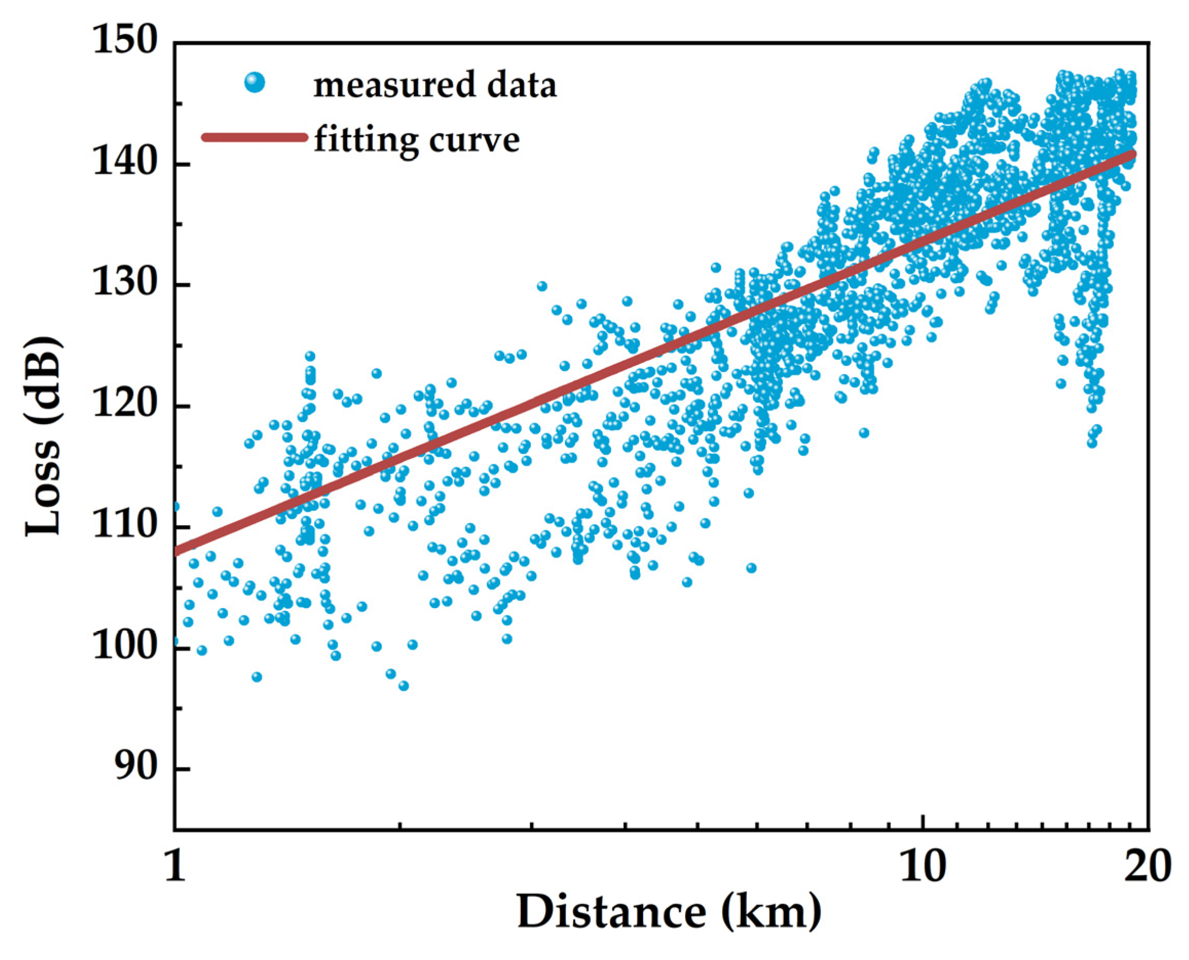
4.4. Measurement Modeling

A curve is fitted from Equation (2), where d is determined by the position of the source and the receive site, and it is the independent variable; L_new is determined by the actual received power, and it is the dependent variable; M and A are the coefficients to be fitted. The results are depicted in Figure 7.

This was fitted by the nonlinear fitting method, and the model parameters are shown in

Table 5. Results of fitting coefficient.

M	A	$\mathit{\chi }$
25.64 (25.05, 26.23)	57.54 (55.85, 59.24)	1.55

. Values in parentheses in the second column denote 95% confidence intervals, and the third column denotes the labeled deviation.

As can be seen from Table 5, the measured statistical model of Wuhan is as follows:

$$L=57.54+25.64\log (d)+25.64\log (f)+\chi$$

(14)

4.5. Discussion

The focus of this subsection is to analyze the three channel types from the transmitting point to the receiving point as well as the modeling of propagation in urban areas. The presence of multiple modes highlights the complexity of radio wave propagation in urban areas, and the proposed method can be applied to a wide range of fields. For example, the method can find applications in the field of atmospheric inversion. By capturing the signal source, it is possible to localize it and analyze its propagation mode and atmospheric environment. By utilizing the proposed techniques, the accuracy of atmospheric inversion can be improved, leading to a better understanding and analysis of atmospheric conditions [38].

5. Conclusions

In this paper, a novel intelligent channel path classification method and a channel modeling method are proposed to address the complexity of the urban electromagnetic environment and the challenge of blind source constraints. The hybrid intelligent method, combining the particle swarm algorithm and genetic algorithm, is used for blind source localization to obtain the location and transmit power information of the radiated source.

A mobile measurement system is constructed based on ambient radio signals, and the proposed method is validated through a comprehensive study using the FM band signals at 92.7 MHz and 95.6 MHz. The study analyzes different channel types, including the LoS, multi-LoS, and NLoS channels. Additionally, propagation models applicable to test point propagation are examined. The proposed method successfully distinguishes the channel types between transmitting and receiving points and demonstrates that the broadcast signal propagation model closely aligns with the actual spatial propagation characteristics of radio waves. These results confirm the effectiveness of the method proposed in this study and suggest the feasibility of using a propagation characterization method based on blind source signals.

Furthermore, the statistical models of urban areas are provided to further characterize the propagation properties based on the measured data. Looking ahead, we expect the field of mobile communication to make new breakthroughs in artificial intelligence and big data. The system presented in this paper can be utilized to confirm the propagation channel paths and model the propagation characteristics of future signals in higher frequency bands [39,40].

References

1. Liu, C.; Xiong, D.; Duan, K.; Hu, W.; Cao, L.; Huang, L.; Guo, X.; Wang, H. Field test investigation on microwave transhorizon propagation over sea surface. Chin. J. Radio Sci. 2022, 37, 214–221. (In Chinese) [Google Scholar]
2. Zhao, X.; Liang, X.; Li, S.; Ai, B. Two-Cylinder and Multi-Ring GBSSM for Realizing and Modeling of Vehicle-to-Vehicle Wideband MIMO Channels. IEEE Trans. Intell. Transp. Syst. 2016, 17, 2787–2799. [Google Scholar] [CrossRef]
3. Wang, J.; Wu, Z.; Hao, Y.; Yang, C.; Shi, Y. An SVR-Based Radio Propagation Prediction Model for Terrestrial FM Broadcasting Services in Beijing and Its Surrounding Area. IEEE Trans. Broadcast. 2023, 13, 1–12. [Google Scholar] [CrossRef]
4. Zhao, X.; Du, F.; Geng, S.; Fu, Z.; Wang, Z.; Zhang, Y.; Zhou, Z.; Zhang, L.; Yang, L. Playback of 5G and Beyond Measured MIMO Channels by an ANN-Based Modeling and Simulation Framework. IEEE J. Sel. Areas Commun. 2020, 38, 1945–1954. [Google Scholar] [CrossRef]
5. Zhao, X.; Abdo, A.M.A.; Xu, C.; Geng, S.; Zhang, J.; Memon, I. Dimension Reduction of Channel Correlation Matrix Using CUR-Decomposition Technique for 3-D Massive Antenna System. IEEE Access 2018, 6, 3031–3039. [Google Scholar] [CrossRef]
6. Tajvidy, A. Diffraction loss model at 0.3–6 GHz for 5G cellular system in microcell urban areas. Electromagnetics 2019, 39, 168–185. [Google Scholar] [CrossRef]
7. Zhang, H. mmWave Indoor Channel Measurement Campaign for 5G New Radio Indoor Broadcasting. Trans. Broadcast. 2022, 68, 331–344. [Google Scholar] [CrossRef]
8. Paul, B.S.; Bhattacharjee, R. MIMO Channel Modeling: A Review. IETE Tech. Rev. 2008, 25, 315–319. [Google Scholar] [CrossRef]
9. Nisirat, M.A.; Ismail, M.; Nissirat, L.; AlKhawaldeh, S.; Yuwono, T. A Hata based model utilizing terrain roughness correction formula. In Proceedings of the 2011 6th International Conference on Telecommunication Systems, Services, and Applications (TSSA), Denpasar, Indonesia,, 20–21 October 2011; pp. 284–287. [Google Scholar]
10. Nisirat, M.A.; Ismail, M.; Nissirat, L.; AlKhawaldeh, S.; Tahbuob, A. Micro cell path loss estimation by means of terrain slope for the 900 and 1800 MHz. In Proceedings of the 2012 International Conference on Computer and Communication Engineering (ICCCE), Kuala Lumpur, Malaysia, 3–5 July 2012; pp. 670–674. [Google Scholar]
11. Castro, B.S.L.; Gomes, I.R.; Ribeiro, F.C.J.; Cavalcante, G.P.S. COST231-Hata and SUI Models performance using a LMS tuning algorithm on 5.8GHz in Amazon Region cities. In Proceedings of the Fourth European Conference on Antennas and Propagation, Barcelona, Spain, 12–16 April 2010; pp. 1–3. [Google Scholar]
12. Levy, M. Parabolic Equation Methods for Electro-Magnetic Wave Propagation; Institution of Engineering and Technology Press: London, UK, 2000; pp. 20–41. [Google Scholar]
13. Son, H.W.; Myung, N.H. A deterministic ray tube method for microcellular wave propagation prediction model. IEEE Trans. Antennas Propag 1999, 47, 1344–1350. [Google Scholar] [CrossRef]
14. Zhao, Y.; Yang, C.; Ji, T.F. Propagation characteristics of 3.6 GHz typical application scenarios based on parabolic equation. Chin. J. Radio Sci. 2021, 36, 604–610. (In Chinese) [Google Scholar]
15. Bender, A. A Flexible System Architecture for Acquisition and Storage of Naturalistic Driving Data. IEEE Trans. Intell. Transp. Syst. 2016, 17, 1748–1761. [Google Scholar] [CrossRef]
16. Duan, K.Y.; Liu, C.G. Automatic mm Wave channel measurement and modeling technology. Comput. Eng. Des. 2022, 43, 1459–1466. (In Chinese) [Google Scholar]
17. Kielgast, M.R.; Rasmussen, A.C.; Laursen, M.H.; Nielsen, J.J.; Popovski, P.; Krigslund, R. Estimation of Received Signal Strength Distribution for Smart Meters with Biased Measurement Data Set. IEEE Wirel. Commun. Lett. 2017, 6, 2–5. [Google Scholar] [CrossRef]
18. Herault, J.; Jutten, C. Space or time adaptive signal processing by neural network models. AIP Conf. Proc. 1986, 151, 206. [Google Scholar]
19. Wang, C.X.; Bian, J.; Sun, J.; Zhang, W.; Zhang, M. A Survey of 5G Channel Measurements and Models. IEEE Commun. Surv. Tutor. 2018, 20, 3142–3168. [Google Scholar] [CrossRef]
20. Liu, P.; Jiang, T. Channel Estimation Performance Analysis of Massive MIMO IoT Systems with Ricean Fading. IEEE Internet Things J. 2021, 8, 6114–6126. [Google Scholar] [CrossRef]
21. Wang, Y.; Lv, Y.; Yin, X.; Duan, J. Measurement-based experimental statistical modeling of propagation channel in industrial IoT scenario. Radio Sci. 2020, 55, 1–14. [Google Scholar] [CrossRef]
22. Wang, X.Y.; Mei, N.; Wang, X.; Fan, X.; Shi, S. Three-Dimensional Channel Modeling and Analysis of Electromagnetic Field for WiFi. In Proceedings of the 2021 13th International Symposium on Antennas, Propagation and EM Theory (ISAPE), Zhuhai, China, 1–4 December 2021; pp. 1–3. [Google Scholar]
23. Wang, J.; Hao, Y.; Yang, C. A Comprehensive Prediction Model for VHF Radio Wave Propagation by Integrating Entropy Weight Theory and Machine Learning Methods. IEEE Trans. Antennas Propag. 2023, 71, 6249–6254. [Google Scholar] [CrossRef]
24. Wang, J.; Hao, Y.; Yang, C. An entropy weight-based method for path loss predictions for terrestrial services in the VHF and UHF bands. Radio Sci. 2023, 58, e2023RS007769. [Google Scholar] [CrossRef]
25. Kong, L.J.; Liu, Y.L.; Zhang, X.C.; Zhang, X.Y.; Zhao, H.T.; Wei, J. Channel measurement and modeling for VHF bands in typical urban scenarios. Chin. J. Radio Sci. 2020, 35, 542–550. (In Chinese) [Google Scholar]
26. Yu, J.; Chen, W.; Li, F.; Li, C.; Yang, K.; Liu, Y.; Chang, F. Channel Measurement and Modeling of the Small-Scale Fading Characteristics for Urban Inland River Environment. IEEE Trans. Wirel. Commun. 2020, 19, 3376–3389. [Google Scholar] [CrossRef]
27. Hata, M. Empirical formula for propagation loss in land mobile radio services. IEEE Trans. Veh. Technol. 1980, 29, 317–325. [Google Scholar] [CrossRef]
28. Egli, J.J. Radio Propagation above 40 MC over Irregular Terrain. Proc. IRE 1957, 45, 1383–1391. [Google Scholar] [CrossRef]
29. Hu, W.T.; Liu, C.G.; Lin, F.J. Characteristics of atmospheric ducts and its impacts on FM broadcasting in Wuhan. Chin. J. Radio Sci. 2020, 35, 856–867. (In Chinese) [Google Scholar]
30. Cao, L.F.; Liu, C.G.; Cheng, R.S. An Optimized PSO Method for EM Radiation Source Positioning. In Proceedings of the National Conference of Microwave and Millimeter Wave 2023 (NCMMW2023), Qingdao, China, 14–17 May 2023. (In Chinese). [Google Scholar]
31. Kennedy, J.; Eberhart, R. Particle swarm optimization. In Proceedings of the ICNN’95—International Conference on Neural Networks, Perth, WA, Australia, 27 November–1 December 1995; pp. 1942–1948. [Google Scholar]
32. Srinivas, M.; Patnaik, L.M. Genetic algorithms: A survey. Computer 1994, 27, 17–26. [Google Scholar] [CrossRef]
33. Bansal, J.C.; Singh, P.K.; Saraswat, M.; Verma, A.; Jadon, S.S.; Abraham, A. Inertia Weight strategies in Particle Swarm Optimization. In Proceedings of the 2011 Third World Congress on Nature and Biologically Inspired Computing, Salamanca, Spain, 19–21 October 2011; pp. 633–640. [Google Scholar]
34. Wu, X.; Zhong, M. Particle Swarm Optimization with Hybrid Velocity Updating Strategies. In Proceedings of the 2009 Third International Symposium on Intelligent Information Technology Application, Nanchang, China, 21–22 November 2009; pp. 336–339. [Google Scholar]
35. Dziwiński, P.; Bartczuk, Ł. A New Hybrid Particle Swarm Optimization and Genetic Algorithm Method Controlled by Fuzzy Logic. IEEE Trans. Fuzzy Syst. 2020, 28, 1140–1154. [Google Scholar] [CrossRef]
36. Ester, M.; Kriegel, H.P.; Sander, J.; Xu, X. A density-based algorithm for discovering clusters in large spatial databases with noise. In KDD-96 Proceedings; AAAI Press: Washington, DC, USA, 1996; Volume 96, pp. 226–231. [Google Scholar]
37. Dupleich, D. Multi-Band Propagation and Radio Channel Characterization in Street Canyon Scenarios for 5G and Beyond. IEEE Access 2019, 7, 160385–160396. [Google Scholar] [CrossRef]
38. Cheng, R.S.; Liu, C.G.; Cao, L.F. The Influence of PE Initial Field Construction Method on Radio Wave Propagation Loss and Tropospheric Duct Inversion. Atmosphere 2024, 15, 46. [Google Scholar] [CrossRef]
39. Wang, J.; Hao, Y.; Yang, C. The Current Progress and Future Prospects of Path Loss Model for Terrestrial Radio Propagation. Electronics 2023, 12, 4959. [Google Scholar] [CrossRef]
40. Wang, J.; Yang, C.; Yan, N.N. Study on digital twin channel for the B5G and 6G communication. Chin. J. Radio Sci. 2021, 36, 340–348. (In Chinese) [Google Scholar]
Figure 1. Complex environment radio wave propagation.
Atmosphere 15 00280 g001
Figure 2. Basic flowchart of PSO_GA.
Atmosphere 15 00280 g002
Figure 3. Hardware system architecture diagram.
Atmosphere 15 00280 g003
Figure 4. Distribution of each channel area. (a) Dataset 1 (b) Dataset 2.
Atmosphere 15 00280 g004
Figure 5. Comparison of datasets with each model. (a) Dataset 1 (b) Dataset 2.
Atmosphere 15 00280 g005
Figure 6. Deviation of the measured data and the deterministic model.
Atmosphere 15 00280 g006
Figure 7. Datasets fitted plot.
Atmosphere 15 00280 g007