Characteristics and Formation Mechanism of Ozone Pollution in Demonstration Zone of the Yangtze River Delta, China

Abstract

Emerging research indicates that ground-level ozone (O₃) has become a leading contributor to air quality concerns in many Chinese cities, with the Yangtze River Delta (YRD) region facing particular challenges. This study investigated the characterization of air pollutants in Wujiang, which is located within the YRD demonstration zone, during the warm season (April–September) of 2022. The contributions of emission and meteorology to O₃ were identified, the O₃-NO_X-VOC sensitivities were discussed, and the VOC sources and their contributions to O₃ formation were analyzed. A random forest model revealed that the high O₃ concentration was mainly caused by a combination of increased emission intensity due to the resumption of work and production after the COVID-19 pandemic, along with adverse meteorological conditions. The results revealed more than 92% of the pollution days were related to O₃ during the warm season, and the impact of O₃ precursor emissions was slightly greater than that of the meteorological conditions. O₃ formation was in the VOC-limited regime, and emission reduction strategies targeting VOCs, particularly aromatics such as toluene and xylene, have been identified as the most effective approach for mitigating O₃ pollution. Changes in O₃-NO_X-VOC sensitivity were also observed from the VOC-limited regime to the transitional regime, which was primarily driven by variations in the NO_X concentrations. The VOC source analysis results showed that the contributions of gasoline vehicle exhaust and diesel engine exhaust (mobile source emissions) were significantly greater than those of the other sources, accounting for 20.8% and 16.5% of the total VOC emissions, respectively. This study highlights the crucial role of mobile source emission control in mitigating O₃ pollution. Furthermore, prioritizing the control of VOC emission sources with minimal NO_X contributions is highly recommended within the VOC-limited regime.

1. Introduction

As a key product of atmospheric photochemical reactions, ozone (O₃) is one of the oxidizing trace gases that exist naturally in the atmosphere [1]. However, elevated ground-level O₃ concentrations pose significant threats to human health, agricultural productivity, and the ecological environment [2,3,4]. Moreover, O₃ ranks as the third most influential greenhouse gas, contributing to global warming [5]. Due to its crucial role in atmospheric chemistry, ecological impacts, and climate change, O₃ has garnered substantial scientific attention.

Starting in 2013, China’s central government launched a series of initiatives aimed at improving air quality [6,7]. A series of stricter emission standards and pollution control measures have been enacted [8,9,10,11], leading to significant improvements in China’s ambient air quality. Notably, fine particulate matter (PM_2.5) concentrations have substantially decreased, along with a significant reduction in the number of days with polluted air. However, a critical challenge persists in the form of regional photochemical pollution, evidenced by the stagnating O₃ concentrations and the growing extent of the polluted area [12,13,14,15]. The concentration of ground-level O₃ is rapidly increasing, which is a critical air quality concern in China, necessitating a shift in focus to future pollution control strategies under the context of declining PM_2.5 concentrations.

The Yangtze River Delta (YRD), a powerhouse of China’s economy, also faces a critical challenge in the form of O₃ pollution [1,14,16]. Currently, O₃ stands as the primary impediment to air quality improvement in the YRD region, making its control the most pressing environmental concern. Some researchers have conducted studies on the sensitivity of O₃ formation and the source of O₃ precursors in the YRD region. The calculation results of using air quality models and observation-based models suggest O₃ formation in the urban areas of the YRD region is in a VOC-limited regime or a transition regime of VOCs and NO_X, and O₃ formation is most sensitive to anthropogenic VOCs, especially alkenes and aromatics [17,18,19,20]. In recent years, the concentration of ambient air pollutants has changed significantly, and the composition and concentration of VOCs and NO_X have obvious inter-year differences in the YRD region. Studies on the concentration changes in O₃ precursors in typical urban areas and their impacts on O₃ pollution remain limited, and this makes it difficult to develop more efficient and refined O₃ control strategies for the YRD region.

To better facilitate the integrated development and implement an eco-green integrated development strategy, the YRD demonstration zone of green and integrated ecological development (demonstration area) was established in 2019 [21]. The demonstration area covers approximately 2300 km² in the Qingpu district of Shanghai city, Wujiang district of Suzhou of Jiangsu province, and Jiashan county of Zhejiang province. This demonstration area is used as a research case to verify the applicability of strategies to improve the eco-environment. A field experiment on air pollutants was conducted in Wujiang, one of the constituent districts in the demonstration area. Monitoring data for O₃ and its precursors collected from April to September of 2022 were employed to analyze the concentration levels and changing characteristics of O₃ and its precursors. This study investigated the contributions of meteorological conditions and pollution source emissions to O₃ concentration and examined the monthly variations in O₃-NO_X-VOCs sensitivities throughout the warm season (April–September). Additionally, VOC sources were identified, and their O₃ formation potentials were calculated. These findings aim to establish a theoretical foundation for O₃ pollution control within the demonstration area.

2. Methods

2.1. Experimental Sites and Periods

This study utilized the monitoring data collected at the VOC monitoring site located in Wujiang, Suzhou, a typical urban area in the demonstration area (Figure 1). The layout of the site complied with the relevant requirements of the Technical Regulation for Selection of Ambient Air Quality Monitoring Stations (on trial) (HJ 664-2013). Situated within a predominantly mixed residential and commercial area and free from significant local air pollution sources, this site is representative of the ambient air quality in the demonstration area and well-suited for the analysis of O₃ pollution characteristics and formation mechanisms.

The ambient VOC concentrations were continuously monitored using an online system equipped with a custom-built cryogen-free cooling device capable of achieving an ultra-low temperature (−165 °C), a dual-channel sampling and pre-concentration unit, and a commercially available gas chromatograph coupled with both a flame ionization detector and mass spectrometer (GC-FID/MS). This system could analyze 29 alkanes, 11 alkenes, 1 acetylene, 17 aromatics, 35 halocarbons, 21 oxygen-containing VOCs (OVOCs) and 1 sulfur-containing VOC (a total of 115 VOCs). The following paper has provided a detailed description of the system [22].

2.2. Data Processing and Analytical Methods

2.2.1. Data Processing

The daily assessment value of O₃ is based on the maximum daily 8 h average concentration of O₃ (MDA8h O₃), while the other pollutants (SO₂, NO₂, CO, PM_2.5 and PM₁₀) were evaluated using their arithmetic means. This evaluation and calculation of the air quality index (AQI) adhere to the Technical Regulation on Ambient Air Quality Index (on trial) (HJ 633-2012) [23]. The concentrations of all the pollutants are reported using standard reference conditions (1 atm, 298.15 K).

2.2.2. Meteorological Normalization Method

Meteorological normalization is a technique used to decouple the influence of meteorology on pollutant concentrations in air quality time series. This approach allows for the quantitative separation of the effects of emissions and meteorological factors on pollutants. Grange et al. [24] first applied the random forest model to the meteorological normalization of pollutants in 2018. The random forest model is an ensemble model consisting of hundreds of independent decision tree models. The bagging algorithm (bootstrap aggregation) used in the model can effectively prevent overfitting during the training process of the random forest model [24,25]. The random forest model takes the hourly data of Unix timestamp (date_unix, the number of seconds since 1 January 1970), Julian date (date_julian), weekday (weekday), hour value (hour), air temperature (Temp), relative humidity (RH), wind speed (WS), wind direction (WD) and pressure (Pres) during the whole observation period as input parameters for training, and can accurately describe the hourly concentration of air pollutants and their input parameter characteristics. The entire dataset is randomly divided into a training dataset for constructing the random forest model and a test dataset for testing the performance of the model. The training dataset includes 70% of all the data, and the remaining data are used as test data. To determine the optimal values of model parameters, such as the number of trees (n_tree), the number of samples (n_sample), and the minimum number of nodes, a series of random forest simulations and model cross-validations were carried out under different model parameters. After obtaining the optimal values of the model parameters, they were input into the model for training. The random sampling process of observation data is automatically repeated 1000 times to generate the final input dataset, and then 1000 datasets are input into the random forest model for 1000 pollutant concentration predictions. A total of 1000 predictions were used to calculate the meteorologically normalized trend. The random forest model was constructed using the “rmweather” package in R by Grange et al. [25].

After meteorological normalization, the new time series represents the pollutant concentration excluding the influence of meteorological factors under the condition of constant emission factors. The difference between the new time series and the actual observed data is the contribution of meteorological influence, which is presented as follows in Equations (1) and (2):

$$M_i=O_i-P_i$$

(1)

$$E_i=O_i-M_i-O_{i-1}$$

(2)

where M_i represents the contribution of meteorological conditions in year i, E_i represents the contribution of emission factors in year i, O_i represents the actual observed concentration of pollutant in year i, and P_i represents the concentration of pollutant after meteorological normalization in year i.

Due to the impact of the COVID-19 (coronavirus disease 2019) pandemic in 2020–2021, this period serves as a suitable reference for pollution levels in 2022. Therefore, by decoupling the impact of meteorological changes on the pollutants, we obtained a more nuanced understanding of how pollution levels during the warm season in 2022 were shaped by both meteorological factors and emission sources.

In this study, the observation data encompass monitoring data from April to June across 2020, 2021 and 2022, totaling 13,078 datasets, which had been audited by relevant government technical departments. All the data were randomly divided into a training set of 9154 datasets and a testing set of 3924 datasets. Only the observations with complete data for both meteorological data and O₃ concentrations were included in the training process. To optimize the model performance and ensure the consistency of input variables, a hyperparameter optimization procedure was employed, and 1000 trees (n_tree) and 3 features considered at each split (mtry) were employed.

It is worth noting that the emission factors in this study included not only changes in primary emissions in the atmosphere, but also secondary pollution caused by changes in emission levels.

2.2.3. Observation-Based Model

This study adopted an observation-based chemical box model (OBM) to quantify the in situ O₃ formation rate and sensitivity to its precursors; the OBM model equipped the Master Chemical Mechanism (MCM, v3.3.1, https://mcm.york.ac.uk/MCM/ accessed on 15 September 2023) offered a comprehensive description of atmospheric chemical processes from emission to decomposition for 143 VOCs species, involving 17,000 inorganic and organic reactions for approximately 6700 species. There were great simulated results in modeling the formation and consumption of O₃ and other secondary gaseous pollutants using the OBM model [26,27,28,29]. Hourly observational data for temperature, humidity, pressure and O₃, NO_X, CO, and VOCs were used as inputs to the OBM to estimate the in situ O₃ formation rate and consumption rate. For the OBM calculations in this study, the Framework for 0-D Atmospheric Modeling (F0AM) was employed [30].

Developed in the 1970s, the empirical kinetics modeling approach (EKMA) was designed to reveal O₃ sensitivity towards VOCs and NO_X to identify mitigation strategies for O₃ precursor emissions [31]. Hourly data were averaged to provide the mean diurnal variation as a base case input for the OBM model. A total of 196 scenarios were established by systematically varying the VOC and NO_X concentrations across a range from 10% to 200% increases and decreases. The isopleths of the maximum O₃ formation rates were generated based on the relationship of O₃-NO_X-VOC. Acknowledging the uncontrollability of biogenic emissions, the EKMA model calculations excluded any scaling of this source [28,32,33].

Here, we used the relative incremental reactivities (RIRs) of different O₃ precursors to analyze the sensitivities of O₃ formation to its precursors [34]. The calculation of RIRs is presented in Equation (3).

$${\mathrm{RIR}}^{\left(\mathrm{s}\right)}\left(\mathrm{X}\right)=\frac{\frac{{\mathrm{P}}_{\mathrm{O}3\mathrm{-NO}}^{\mathrm{s}}\left(\mathrm{X}\right)-{\mathrm{P}}_{\mathrm{O}3\mathrm{-NO}}^{\mathrm{s}}\left(\left[\mathrm{X}\right]-\mathsf{\Delta }\left[\mathrm{X}\right]\right)}{{\mathrm{P}}_{\mathrm{O}3\mathrm{-NO}}^{\mathrm{s}}\left(\mathrm{X}\right)}}{\frac{\mathsf{\Delta }\mathrm{S}\left(\mathrm{X}\right)}{\mathrm{S}\left(\mathrm{X}\right)}}$$

(3)

where ${\mathrm{P}}_{\mathrm{O}3\mathrm{-NO}}\left(\mathrm{X}\right)$ is the mean formation rate of the O₃ precursor (X) from 8:00 to 18:00, and the relative change in the precursor (ΔS(X)/S(X)) was set at 20%. The RIRs of the O₃ precursors (including NO_X, CO, anthropogenic VOCs (AHC) and biogenic VOCs (BHC)) were calculated. The RIRs of the different VOC categories (including alkanes, alkenes, alkyne, aromatics, halocarbons and OVOCs) were also calculated to precisely assess the sensitivity of O₃ formation to AHC.

2.2.4. O₃ Formation Potential

To assess the contributions of VOCs to O₃ formation potential (OFP), the concept of maximum incremental reactivity (MIR) was studied, as detailed in Equation (4).

$$\mathrm{OFP}={\displaystyle \sum }{\mathrm{MIR}}_{\mathrm{i}}\times \left[{\mathrm{VOC}}_{\mathrm{i}}\right]$$

(4)

where [VOC_i] and OFP are the mass concentration (in μg/m³).

2.2.5. Positive Matrix Factorization (PMF) Model

VOC source apportionment was performed on the measured concentrations using positive matrix factorization (PMF, version 5.0) [35]. We evaluated the model robustness by examining the Q_robust/Q_expected change rates for different factor solutions. As the number of factors increases, a decrease in the rate of change for these values indicates the overfitting of data [36,37,38].

Based on the observed VOC characteristics and source emission profiles within the demonstration area, the tracer species exhibiting representative source contributions and obvious temporal variations were selected for source analysis. The ozone formation potentials (OFPs) of these identified VOC sources were calculated to evaluate their maximum potential contribution to O₃ formation.

3. Results and Discussion

3.1. Overall Characteristics of O₃ Pollution

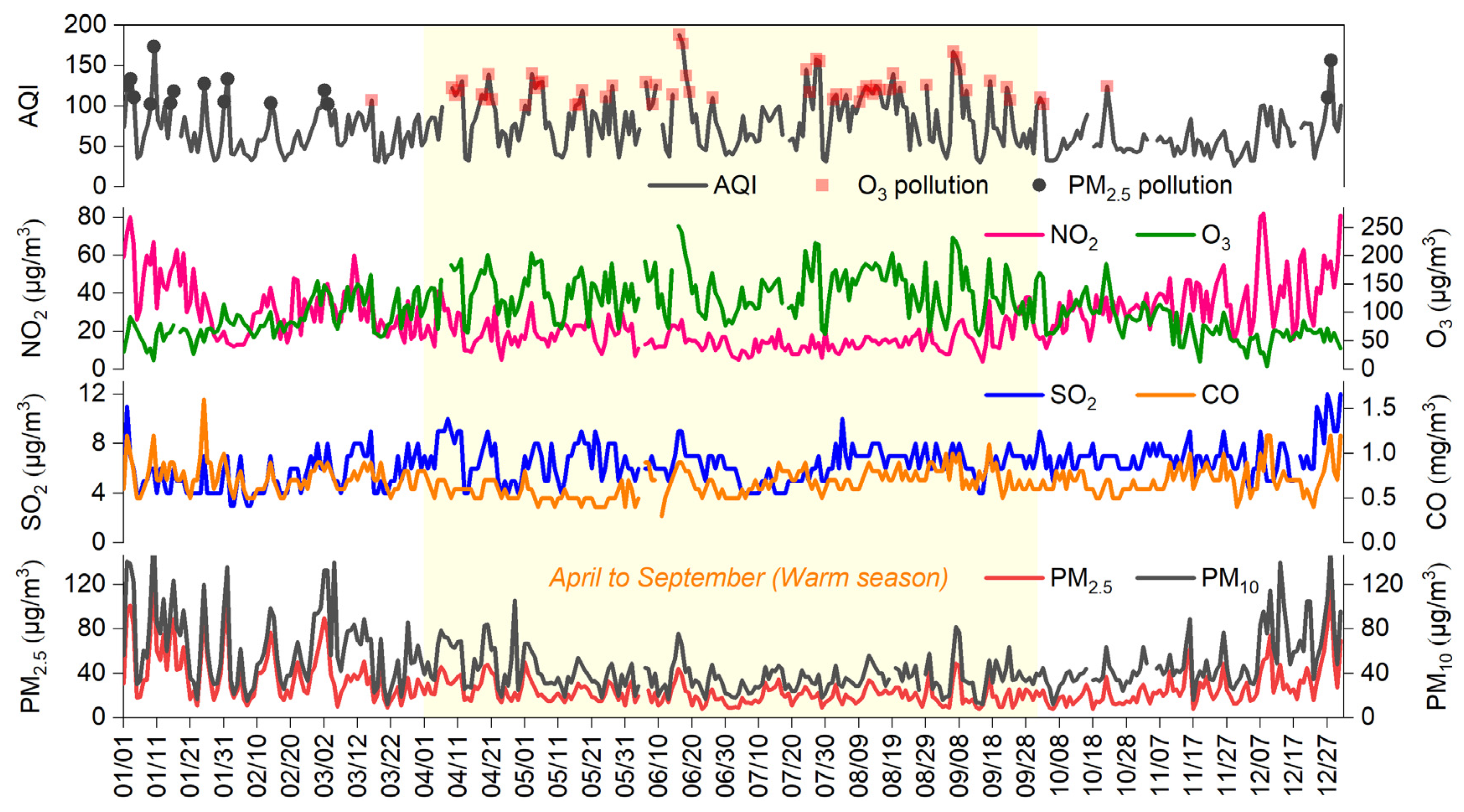
During 2022, Wujiang experienced a total of 73 pollution days, during which O₃ was polluted on 56 days (76.7% of the total pollution days) (Figure 2), highlighting its emergence as the most concerning ambient air quality issue in the district. Fifty-two (92%) of these O₃ pollution days occurred during the warm season, characterized by higher temperatures and less humidity, which promote enhanced atmospheric photochemical reactions. Adverse meteorological conditions or elevated O₃ precursor concentrations can further exacerbate O₃ formation. Therefore, in the following analysis of O₃ formation sensitivity and VOC source apportionment, this study focused on observational data in the warm season (April–September) in 2022.

3.2. Contributions of Meteorological Factors and Emission Factors to O₃

The deweathered and detrended data were used to better understand how the air quality responds to changes in source emissions and meteorological conditions.

The assessment of the effectiveness of the proposed machine learning models involves the evaluation of a comprehensive set of performance metrics, including the determination coefficient (R²), root-mean-square error (RMSE), and normalized mean bias (NMB), which are given in Equation (5), Equation (6), and Equation (7), respectively. Here,$y_i^{\prime }$represents prediction, $y_i$represents observation, and $\overline{y}$represents the average value of $y_i$.

$$R^2=\frac{{{\displaystyle \sum }}_{i=1}^n{\left(y_i^{\prime }-\overline{y}\right)}^2}{{{\displaystyle \sum }}_{i=1}^n{\left(y_i-\overline{y}\right)}^2}$$

(5)

$$\mathrm{RMSE}=\sqrt{\frac{1}{n}{{\displaystyle \sum }}_{i=1}^n{\left(y_i^{\prime }-\overline{y}\right)}^2}$$

(6)

$$\mathrm{NMB}=\frac{{{\displaystyle \sum }}_{i=1}^n{\left(y_i^{\prime }-\overline{y}\right)}^2}{{{\displaystyle \sum }}_{i=1}^n{y}_i}$$

(7)

The statistical metrics of our random forest model simulation of pollutants are as follows—R² value: 0.94; RMSE: 12.99 μg/m³; and NMB: 9 × 10⁻⁴. The results confirm that the simulation of the model is good and demonstrate the suitability of further applications.

After the procedure of meteorological normalization, the O₃ daily average concentrations (arithmetic means) during the warm seasons of 2020, 2021 and 2022 in Wujiang were 87, 86 and 89 μg/m³, respectively, while the observed values were 84, 82 and 95 μg/m³, respectively. From Equations (1) and (2), it can be calculated that, in 2022, due to adverse meteorological conditions, the concentration of O₃ increased by 5 μg/m³ (5.7%), and due to emission factors, the concentration of O₃ increased by 7 μg/m³ (7.7%). Therefore, the high O₃ concentration in the warm season of 2022 was caused by the superposition of adverse meteorological conditions and increased emission intensity from the resumption of work and production after the implementation of the dynamic zero COVID-19 guidelines during the pandemic, in which the emission factors were slightly greater than the meteorological factors.

3.3. O₃-NO_X-VOC Sensitivity

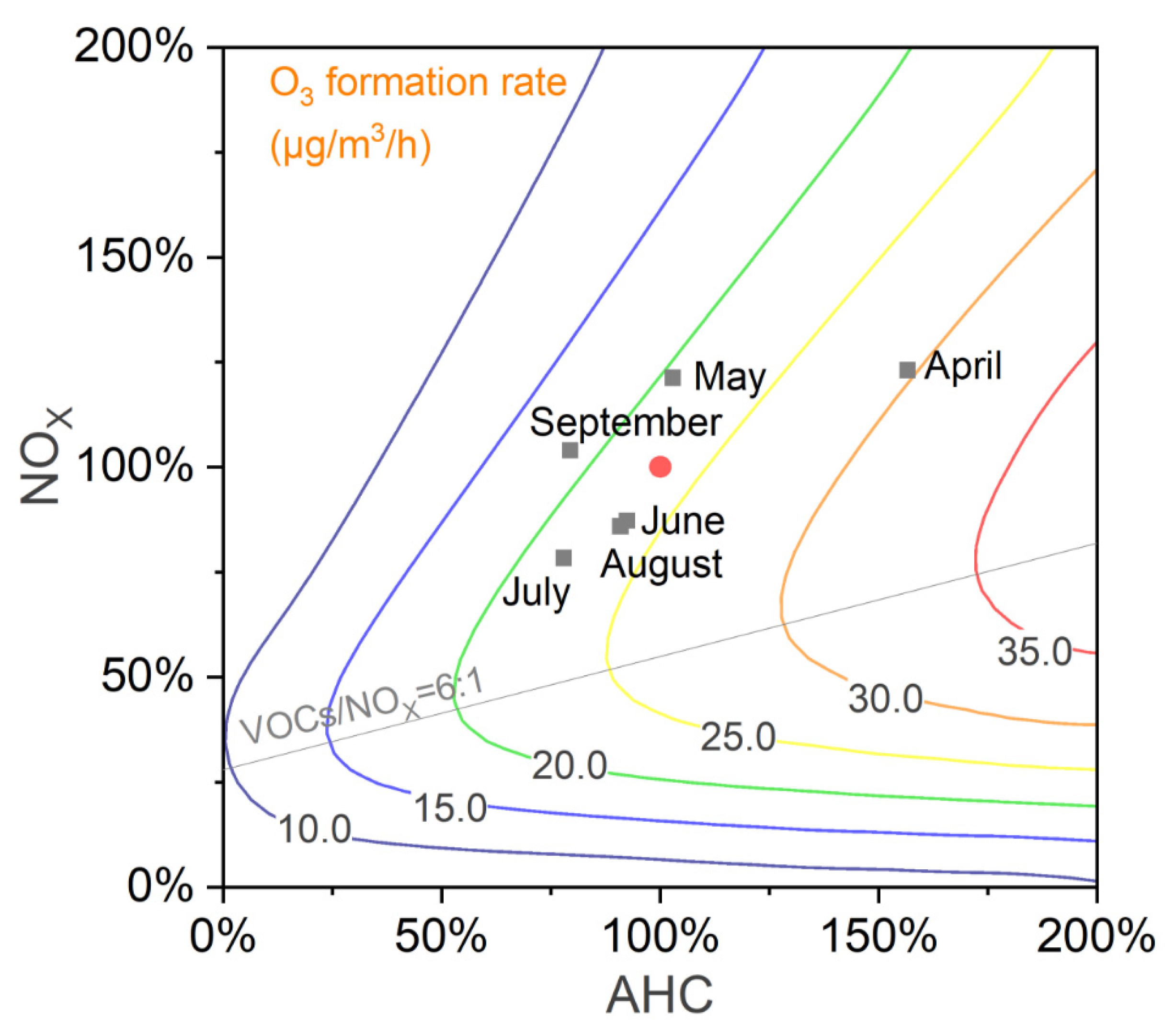
This study employed the OBM to calculate the net in situ O₃ formation rate as a function of NOx and anthropogenic VOC (AHC) reactivities during the warm season. The results are presented as an isopleth diagram. The results indicated that O₃-NO_X-VOC sensitivity was in the VOC-limited regime. O₃ formation exhibited the greatest sensitivity to VOCs, and emission reduction focused on VOCs could be the most effective strategy for mitigating O₃ pollution. Reducing the NO_X concentrations could weaken the NO_X titration effect, potentially leading to the unintended enhancement of O₃ formation. Thus, NO_X emission reduction may not be the optimal strategy for mitigating O₃ pollution in the short term.

From the perspective of different months during the warm season, April exhibited the highest O₃ formation potential, with a formation rate approaching 30 micrograms per cubic meter per hour (μg/m³/h), coinciding with elevated concentrations of the O₃ precursors. From May to July, both the VOC and NO_X concentrations showed a monthly decreased trend. Especially in July, those of VOC and NO_X dropped by 50% and 64% more than those in April, respectively. This decrease was also accompanied by a significant decline in the O₃ formation rate (approximately 22 μg/m³/h). Compared with those in July, the VOC and NO_X concentrations rose slightly more in August. In September, the VOC concentration maintained at a similar level to that in July and August, but the NO_X concentration increased significantly. Notably, the September increase in NO_X concentration led to a substantial reduction in the O₃ formation rate (Figure 2 and Figure 3). Overall, in the warm season of 2022, the changes in O₃ formation regime were mainly driven by the variations in NO_X concentration and less by the VOCs (Figure 4). While both NO_X and the VOCs are key precursors of PM_2.5 and O₃, a coordinated reduction strategy remains crucial. The isopleth diagram shows a value of approximately six for the VOCs and NO_X, suggesting that control strategies prioritizing VOC reductions should maintain a ratio of six or higher for optimal O₃ mitigation in the demonstration area.

3.4. RIR Analysis of O₃ Precursors

According to the sensitivity analysis of O₃ formation (Figure 5), O₃ formation in the demonstration area was in the VOC-limited regime, although exhibiting slight monthly variations. The O₃ formation sensitivities in April, May and September were in the strong VOC-limited regime. The O₃ formation sensitivities shifted towards the weak VOC-limited regime from June to August, implying that the titration effect of NO_X for O₃ formation is neglected. However, the contribution of anthropogenic VOCs to O₃ formation consistently displayed the highest across all the months, while the contributions of biogenic VOCs and carbon monoxide were relatively minor.

In terms of various VOC species, aromatics originating from anthropogenic VOC sources emerged as the most significant contributors to O₃ formation, followed by alkenes. Alkanes and OVOCs also exhibited a certain level of contribution. This study further investigated the O₃ formation sensitivity to typical high-reactive VOCs (including ethylene, propylene, toluene and xylene); the results show that toluene and xylene contributed significantly to O₃ formation, followed by ethylene and propylene. The total RIRs of toluene and xylene were slightly lower than those of the aromatics, and the similar contributions of ethylene and propylene to alkenes also mean that the specifically high-reactive VOCs species were the dominated compounds for O₃ formation. These findings suggested that prioritizing the control of aromatics, particularly toluene and xylene, is crucial for mitigating O₃ pollution in the demonstration area. Concurrently, coordinated control strategies targeting alkenes, especially ethylene and propylene, are also recommended.

3.5. Source Analysis of VOCs

The observed VOC concentrations were input into the PMF model for source allocation. This analysis identified seven distinct source profiles, including gasoline evaporation, gasoline vehicle exhaust and industrial emissions, solvent use, biogenic emissions, diesel engine exhaust and fossil fuel combustion.

The identification of VOC sources relies on specific tracer species (Figure 6). Large contributions of propane, n-pentane and iso-pentane indicate gasoline evaporation, with this source exhibiting pronounced diurnal variations characterized by higher concentrations during the day and lower concentrations at night [39]. Low-carbon alkenes, such as propylene and 1-butene, are primarily associated with gasoline vehicle exhaust [40]. Industrial emissions are distinguished by the dominance of n-butane and benzene, along with a notable presence of other alkanes [41]. Toluene is a key tracer for solvent use, reflecting its widespread application as an organic solvent [41,42]. Biogenic emissions are identified by the presence of isoprene, which exhibits peak concentrations during the daytime, reflecting its light-dependent production processes [43,44]. Due to the well-developed water transport network and the frequent use of off-road machinery in factories and construction in the demonstration area, the diesel engines in this study are composed of diesel trucks, diesel off-road machinery and inland vessels. Diesel engine combustion is distinguished by the high proportion of propane and m/p-xylene, along with the elevated proportion of n-heptane and ethylbenzene, all of which are known to be abundant in diesel combustion [45,46,47]. Fossil fuel combustion is identified by the relatively high ratio of acetylene to benzene [48,49].

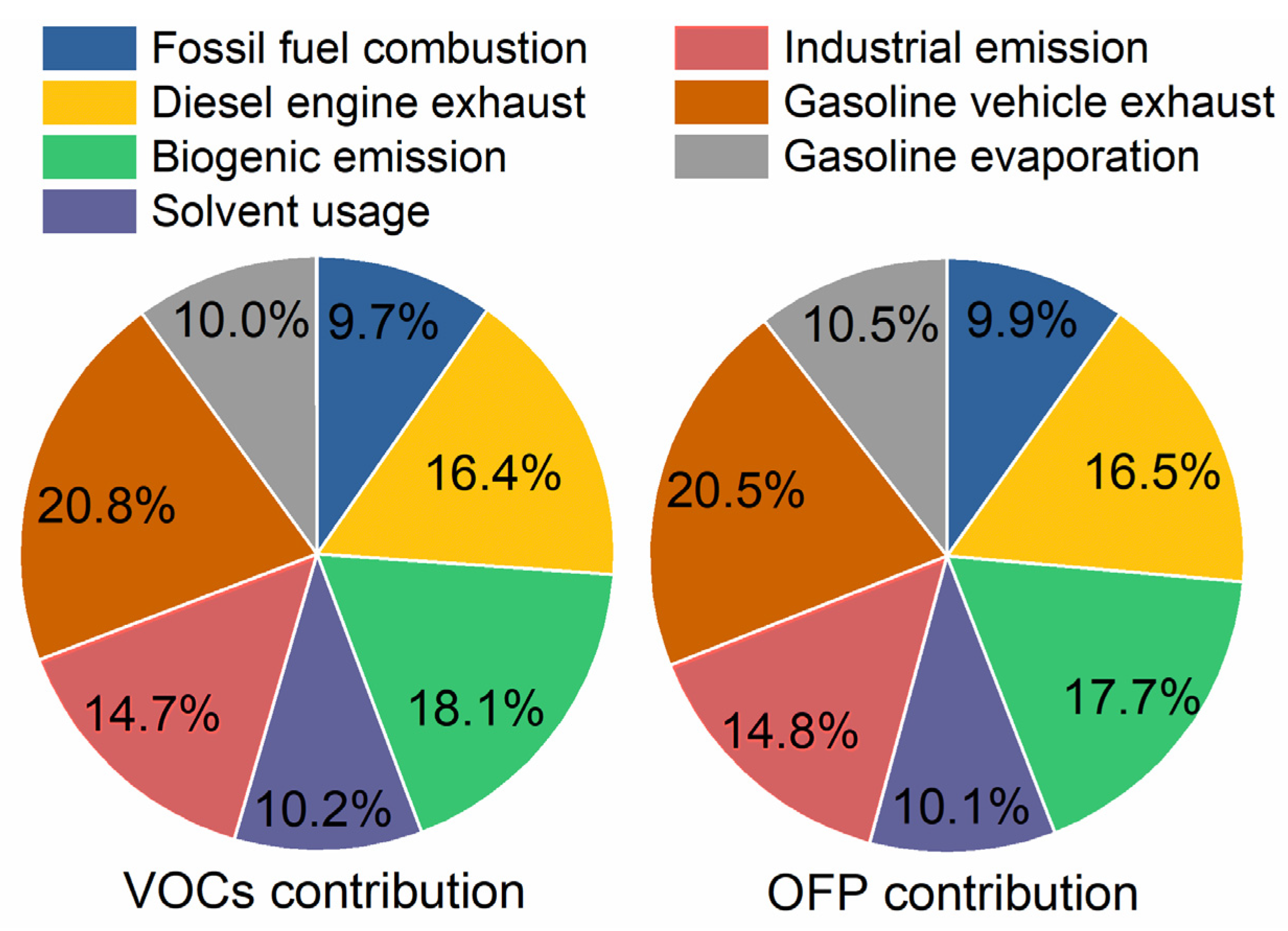
The source apportionment of VOCs (Figure 7) showed that gasoline vehicle exhaust are the most prominent contributor (20.8%), likely attributable to the extensive vehicle population and well-developed road traffic network in the demonstration area. The contributions of biogenic emissions and diesel engine exhaust to VOCs ranked in the second and third positions (18.1% and 16.5%), followed by industrial emissions (14.7%). The relatively high vegetation coverage in the demonstration area contributed to the higher biogenic VOC contribution compared to the Suzhou average [27]. Solvent use, gasoline evaporation and fossil fuel combustion exhibited similar contributions, ranging from 9.7% to 10.2%. Notably, mobile sources (gasoline and diesel vehicle exhaust) constituted the largest contributor to VOC emissions, accounting for 37.3%.

This study redistributed the contributions of the VOC species in each emission source according to their MIR value and calculated the OFP contributions of the VOC emission sources. On the whole, the OFP contributions of all the emission sources were 20.5%, 17.7%, 16.5%, 14.8%, 10.5%, 10.1% and 9.9% from the highest to the lowest for gasoline vehicle exhaust, biogenic emission, diesel engine exhaust, industrial emission, gasoline evaporation, solvent use and fossil fuel combustion, respectively. Compared with the proportion of each source in concentration analysis, the proportion of fossil fuel combustion, industrial emissions and gasoline evaporation increased, indicating that the VOCs emitted from the above three sources had higher reactivity. Comprehensive analysis emphasizes the critical need for prioritizing control strategies that target VOC emissions from gasoline vehicles and diesel engines (trucks, off-road machinery and inland vessels) for effective O₃ pollution mitigation, which is similar to the findings of other studies [27,50,51]. Additionally, controlling the VOC sources from solvent use and gasoline evaporation, which are characterized by minimal NO_X contributions, can provide additional environmental benefits beyond O₃ mitigation.

4. Conclusions

This study investigated the characteristics of air pollutants in Wujiang, one of three areas within the demonstration zone of the YRD region, during the warm season (April–September) in 2022. The findings revealed that O₃ has become the most critical pollutant, and more than 92% of pollution days are O₃ pollution days during the warm season.

A random forest model revealed that adverse meteorological conditions contributed 5 μg/m³ (5.7%) to the increase in O₃ concentration, while the pollution source emissions played a slightly larger role, contributing 7 μg/m³ (7.7%) to the increase in the O₃ concentration. The high O₃ concentration was mainly caused by a combination of increased emission intensity due to the resumption of work and production after the COVID-19 pandemic, along with adverse meteorological conditions. The impact of emission factors was slightly greater than that of the meteorological conditions.

O₃-NO_X-VOC sensitivity occurred in the VOC-limited regime during the warm season. The reduction of VOC emissions is the most effective method for O₃ control, particularly aromatics and alkenes, while NO_X emission reduction is not conducive to mitigate O₃ pollution. Changes in O₃-NO_X-VOC sensitivity were observed from the VOC-limited regime to the transitional regime, primarily driven by variations in the NO_X concentrations and less by the VOCs.

The VOC source analysis results showed that the contribution of gasoline vehicle exhaust and diesel engine exhaust (trucks, off-road machinery and inland vessels) were significantly higher than those of the other sources, accounting for 20.8% and 16.5%, respectively, of the total VOC emissions. Therefore, prioritizing the control strategies targeting mobile VOC emissions (gasoline vehicle and diesel engine exhaust) are crucial for mitigating O₃ pollution. Furthermore, it is suggested that the emission sources with minimal NO_X contributions should be controlled under the VOC-limited regime.

References

- Wang, T.; Xue, L.; Brimblecombe, P.; Lam, Y.F.; Li, L.; Zhang, L. Ozone pollution in China: A review of concentrations, meteorological influences, chemical precursors, and effects. Sci. Total Environ. 2017, 575, 1582. [Google Scholar] [CrossRef]
- Mirowsky, J.E.; Carraway, M.S.; Dhingra, R.; Tong, H.; Neas, L.; Diaz-Sanchez, D.; Cascio, W.; Case, M.; Crooks, J.; Hauser, E.R.; et al. Ozone exposure is associated with acute changes in inflammation, fibrinolysis, and endothelial cell function in coronary artery disease patients. Environ. Health 2017, 16, 126. [Google Scholar] [CrossRef]
- Ruan, Z.; Qian, Z.M.; Guo, Y.; Zhou, J.; Yang, Y.; Acharya, B.K.; Guo, S.; Zheng, Y.; Cummings-Vaughn, L.A.; Rigdon, S.E.; et al. Ambient fine particulate matter and ozone higher than certain thresholds associated with myopia in the elderly aged 50 years and above. Environ. Res. 2019, 177, 108581. [Google Scholar] [CrossRef]
- Feng, Z.; Hu, E.; Wang, X.; Jiang, L.; Liu, X. Ground-level O3 pollution and its impacts on food crops in China: A review. Environ. Pollut. 2015, 199, 42–48. [Google Scholar] [CrossRef]
- IPCC. Climate Change 2023: Synthesis Report; IPCC: Geneva, Switzerland, 2023.
- The Central People’s Government of the People’s Republic of China. Air Pollution Prevention and Control Action Plan. Available online: http://www.gov.cn/zwgk/2013-09/12/content_2486773.htm (accessed on 12 September 2013).
- The Central People’s Government of the People’s Republic of China. Circular of the State Council on Printing and Issuing the Three-year Action Plan for Fighting to Win the Battle against Air Pollution. Available online: http://www.gov.cn/zhengce/content/2018-07/03/content_5303158.htm (accessed on 3 July 2018).
- Zhang, Q.; Zheng, Y.; Tong, D.; Shao, M.; Wang, S.; Zhang, Y.; Xu, X.; Wang, J.; He, H.; Liu, W.; et al. Drivers of improved PM2.5 air quality in China from 2013 to 2017. Proc. Natl. Acad. Sci. USA 2019, 116, 24463–24469. [Google Scholar] [CrossRef]
- Wu, Y.; Zhang, S.; Hao, J.; Liu, H.; Wu, X.; Hu, J.; Walsh, M.P.; Wallington, T.J.; Zhang, K.M.; Stevanovic, S. On-road vehicle emissions and their control in China: A review and outlook. Sci. Total Environ. 2017, 574, 332–349. [Google Scholar] [CrossRef]
- Tang, L.; Qu, J.; Mi, Z.; Bo, X.; Chang, X.; Anadon, L.; Wang, S.; Xue, X.; Li, S.; Wang, X.; et al. Substantial emission reductions from Chinese power plants after the introduction of ultra-low emissions standards. Nat. Energy 2019, 4, 929–938. [Google Scholar] [CrossRef]
- The Central People’s Government of the People’s Republic of China. Air Pollution Prevention Group Revamped. Available online: http://www.gov.cn/zhengce/content/2018-07/11/content_5305678.htm (accessed on 11 July 2018).
- Sun, L.; Xue, L.; Wang, T.; Gao, J.; Ding, A.; Cooper, O.R.; Lin, M.; Xu, P.; Wang, Z.; Wang, X.; et al. Significant increase of summertime ozone at Mount Tai in Central Eastern China. Atmos. Chem. Phys. 2016, 16, 10637–10650. [Google Scholar] [CrossRef]
- Ma, Z.; Xu, J.; Quan, W.; Zhang, Z.; Lin, W.; Xu, X. Significant increase of surface ozone at a rural site, north of eastern China. Atmos. Chem. Phys. 2016, 16, 3969–3977. [Google Scholar] [CrossRef]
- Lu, X.; Zhang, L.; Wang, X.; Gao, M.; Li, K.; Zhang, Y.; Yue, X.; Zhang, Y. Rapid Increases in Warm-Season Surface Ozone and Resulting Health Impact in China Since 2013. Environ. Sci. Technol. Lett. 2020, 7, 240–247. [Google Scholar] [CrossRef]
- Li, K.; Jacob, D.J.; Liao, H.; Shen, L.; Zhang, Q.; Bates, K.H. Anthropogenic drivers of 2013-2017 trends in summer surface ozone in China. Proc. Natl. Acad. Sci. USA 2019, 116, 422–427. [Google Scholar] [CrossRef] [PubMed]
- Wang, T.; Xue, L.; Feng, Z.; Dai, J.; Zhang, Y.; Tan, Y. Ground-level ozone pollution in China: A synthesis of recent findings on influencing factors and impacts. Environ. Res. Lett. 2022, 17, 063003. [Google Scholar] [CrossRef]
- Tan, Y.; Wang, T. What caused ozone pollution during the 2022 Shanghai lockdown? Insights from ground and satellite observations. Atmos. Chem. Phys. 2022, 22, 14455–14466. [Google Scholar] [CrossRef]
- Li, X.; Qin, M.; Li, L.; Gong, K.; Shen, H.; Li, J.; Hu, J. Examining the implications of photochemical indicators for O3–NOx–VOC sensitivity and control strategies: A case study in the Yangtze River Delta (YRD), China. Atmos. Chem. Phys. 2022, 22, 14799–14811. [Google Scholar] [CrossRef]
- Wang, H.; Liu, Y.; Chen, X.; Gao, Y.; Qiu, W.; Jing, S.; Wang, Q.; Lou, S.; Edwards, P.M.; Huang, C.; et al. Unexpected fast radical production emerges in cool seasons: Implications for ozone pollution control. Natl. Sci. Open 2022, 1, 20220013. [Google Scholar] [CrossRef]
- Wang, H.; Huang, C.; Tao, W.; Gao, Y.; Wang, S.; Jing, S.; Wang, W.; Yan, R.; Wang, Q.; An, J.; et al. Seasonality and reduced nitric oxide titration dominated ozone increase during COVID-19 lockdown in eastern China. Npj Clim. Atmos. Sci. 2022, 5, 24. [Google Scholar] [CrossRef]
- The State Council’s Approval to the Overall Plan of the Demonstration Zone of Green and Integrated Ecological Development of Yangtze River Delta. Available online: https://www.gov.cn/zhengce/content/2019-10/29/content_5446300.htm (accessed on 29 October 2019).
- Wang, M.; Zeng, L.; Lu, S.; Shao, M.; Liu, X.; Yu, X.; Chen, W.; Yuan, B.; Zhang, Q.; Hu, M.; et al. Development and validation of a cryogen-free automatic gas chromatograph system (GC-MS/FID) for online measurements of volatile organic compounds. Anal. Methods 2014, 6, 9424–9434. [Google Scholar] [CrossRef]
- MEE. Technical Regulation on Ambient Air Quality Index (on Trial); China Environmental Science Press: Beijing, China, 2012. [Google Scholar]
- Grange, S.K.; Carslaw, D.C.; Lewis, A.C.; Boleti, E.; Hueglin, C. Random forest meteorological normalisation models for Swiss PM10 trend analysis. Atmos. Chem. Phys. 2018, 18, 6223–6239. [Google Scholar] [CrossRef]
- Wang, Y.; Wen, Y.; Wang, Y.; Zhang, S.; Zhang, K.M.; Zheng, H.; Xing, J.; Wu, Y.; Hao, J. Four-Month Changes in Air Quality during and after the COVID-19 Lockdown in Six Megacities in China. Environ. Sci. Technol. Lett. 2020, 7, 802–808. [Google Scholar] [CrossRef]
- Zhang, X.; Li, H.; Wang, X.; Zhang, Y.; Bi, F.; Wu, Z.; Liu, Y.; Zhang, H.; Gao, R.; Xue, L.; et al. Heavy ozone pollution episodes in urban Beijing during the early summertime from 2014 to 2017: Implications for control strategy. Environ. Pollut. 2021, 285, 117162. [Google Scholar] [CrossRef]
- Zhang, X.; Ma, Q.; Chu, W.; Ning, M.; Liu, X.; Xiao, F.; Cai, N.; Wu, Z.; Yan, G. Identify the key emission sources for mitigating ozone pollution: A case study of urban area in the Yangtze River Delta region, China. Sci. Total Environ. 2023, 892, 164703. [Google Scholar] [CrossRef]
- Tan, Z.; Lu, K.; Dong, H.; Hu, M.; Li, X.; Liu, Y.; Lu, S.; Shao, M.; Su, R.; Wang, H.; et al. Explicit diagnosis of the local ozone production rate and the ozone-NOx-VOC sensitivities. Sci. Bull. 2018, 63, 1067–1076. [Google Scholar] [CrossRef]
- Shen, H.; Liu, Y.; Zhao, M.; Li, J.; Zhang, Y.; Yang, J.; Jiang, Y.; Chen, T.; Chen, M.; Huang, X.; et al. Significance of carbonyl compounds to photochemical ozone formation in a coastal city (Shantou) in eastern China. Sci. Total Environ. 2021, 764, 144031. [Google Scholar] [CrossRef] [PubMed]
- Wolfe, G.M.; Marvin, M.R.; Roberts, S.J.; Travis, K.R.; Liao, J. The Framework for 0-D Atmospheric Modeling (F0AM) v3.1. Geosci. Model Dev. 2016, 9, 3309–3319. [Google Scholar] [CrossRef]
- Dodge, M.C. Proceedings of the International Conference on Photochemical Oxidant Pollution and Its Control; USEPA: Research Triangle Park, NC, USA, 1977; Volume II, pp. 881–889. [Google Scholar]
- He, Z.; Wang, X.; Ling, Z.; Zhao, J.; Guo, H.; Shao, M.; Wang, Z. Contributions of different anthropogenic volatile organic compound sources to ozone formation at a receptor site in the Pearl River Delta region and its policy implications. Atmos. Chem. Phys. 2019, 19, 8801–8816. [Google Scholar] [CrossRef]
- Yu, D.; Tan, Z.; Lu, K.; Ma, X.; Li, X.; Chen, S.; Zhu, B.; Lin, L.; Li, Y.; Qiu, P.; et al. An explicit study of local ozone budget and NOx-VOCs sensitivity in Shenzhen China. Atmos. Environ. 2020, 224, 117304. [Google Scholar] [CrossRef]
- Cardelino, C.A.; Chameides, W.L. An observation-based model for analyzing ozone precursor relationships in the urban atmosphere. J. Air Waste Manag. Assoc. 1995, 45, 161–180. [Google Scholar] [CrossRef] [PubMed]
- U. S. Environmental Protection Agency. EPA Positive Matrix Factorization (PMF) 5.0 Fundamentals and User Guide; U.S. Environmental Protection Agency: Washington, DC, USA, 2014.
- Liu, B.; Liang, D.; Yang, J.; Dai, Q.; Bi, X.; Feng, Y.; Yuan, J.; Xiao, Z.; Zhang, Y.; Xu, H. Characterization and source apportionment of volatile organic compounds based on 1-year of observational data in Tianjin, China. Environ. Pollut. 2016, 218, 757–769. [Google Scholar] [CrossRef]
- Li, Y.; Gao, R.; Xue, L.; Wu, Z.; Yang, X.; Gao, J.; Ren, L.; Li, H.; Ren, Y.; Li, G.; et al. Ambient volatile organic compounds at Wudang Mountain in Central China: Characteristics, sources and implications to ozone formation. Atmos. Res. 2021, 250, 105359. [Google Scholar] [CrossRef]
- Liu, Y.; Song, M.; Liu, X.; Zhang, Y.; Hui, L.; Kong, L.; Zhang, Y.; Zhang, C.; Qu, Y.; An, J.; et al. Characterization and sources of volatile organic compounds (VOCs) and their related changes during ozone pollution days in 2016 in Beijing, China. Environ. Pollut. 2020, 257, 113599. [Google Scholar] [CrossRef]
- Sun, L.; Zhong, C.; Peng, J.; Wang, T.; Wu, L.; Liu, Y.; Sun, S.; Li, Y.; Chen, Q.; Song, P.; et al. Refueling emission of volatile organic compounds from China 6 gasoline vehicles. Sci. Total Environ. 2021, 789, 147883. [Google Scholar] [CrossRef] [PubMed]
- Sha, Q.E. Methodological Improvement on Speciated Volatile Organic Compunds (VOCs) Emission Inventory and Reactivity Assessment: A Case Study of On-Road Mobile Source; South China University of Technology: Guangzhou, China, 2019. [Google Scholar]
- Wang, H.; Yang, Z.; Jing, S. Volatile Organic Compounds (VOCs) Source Profiles of Industrial Processing and Solvent Use Emissions: A Review. Environ. Sci. 2017, 38, 2617–2628. (In Chinese) [Google Scholar] [CrossRef]
- Cho, M.; Kim, K.-H.; Szulejko, J.E.; Dutta, T.; Jo, S.-H.; Lee, M.-H.; Lee, S.-h. Paint booth volatile organic compounds emissions in an urban auto-repair center. Anal. Sci. Technol. 2017, 30, 329–337. [Google Scholar] [CrossRef]
- Xie, X.; Shao, M.; Liu, Y.; Lu, S.; Chang, C.-C.; Chen, Z.-M. Estimate of initial isoprene contribution to ozone formation potential in Beijing, China. Atmos. Environ. 2008, 42, 6000–6010. [Google Scholar] [CrossRef]
- Cheng, X.; Li, H.; Zhang, Y.; Li, Y.; Zhang, W.; Wang, X.; Bi, F.; Zhang, H.; Gao, J.; Chai, F.; et al. Atmospheric isoprene and monoterpenes in a typical urban area of Beijing: Pollution characterization, chemical reactivity and source identification. J. Environ. Sci. 2018, 71, 150–167. [Google Scholar] [CrossRef] [PubMed]
- Sha, Q.e.; Zhu, M.; Huang, H.; Wang, Y.; Huang, Z.; Zhang, X.; Tang, M.; Lu, M.; Chen, C.; Shi, B.; et al. A newly integrated dataset of volatile organic compounds (VOCs) source profiles and implications for the future development of VOCs profiles in China. Sci. Total Environ. 2021, 793, 148348. [Google Scholar] [CrossRef] [PubMed]
- Yao, Z.; Shen, X.; Ye, Y.; Cao, X.; Jiang, X.; Zhang, Y.; He, K. On-road emission characteristics of VOCs from diesel trucks in Beijing, China. Atmos. Environ. 2015, 103, 87–93. [Google Scholar] [CrossRef]
- Wang, R.; Yuan, Z.; Zheng, J.; Li, C.; Huang, Z.; Li, W.; Xie, Y.; Wang, Y.; Yu, K.; Duan, L. Characterization of VOC emissions from construction machinery and river ships in the Pearl River Delta of China. J. Environ. Sci. 2020, 96, 138–150. [Google Scholar] [CrossRef]
- Zhang, H.; Li, H.; Zhang, Q.; Zhang, Y.; Zhang, W.; Wang, X.; Bi, F.; Chai, F.; Gao, J.; Meng, L.; et al. Atmospheric Volatile Organic Compounds in a Typical Urban Area of Beijing: Pollution Characterization, Health Risk Assessment and Source Apportionment. Atmosphere 2017, 8, 61. [Google Scholar] [CrossRef]
- Geng, C.; Yang, W.; Sun, X.; Wang, X.; Bai, Z.; Zhang, X. Emission factors, ozone and secondary organic aerosol formation potential of volatile organic compounds emitted from industrial biomass boilers. J. Environ. Sci. 2019, 83, 64–72. [Google Scholar] [CrossRef]
- Wu, Y.; Zhang, X.; Gu, J.; Miao, Q.; Wei, H.; Xiong, Y.; Yang, Q.; Wu, B.; Shen, W.; Ma, Q. Ozone Pollution in Suzhou during Early Summertime: Formation Mechanism and Interannual Variation. Environ. Sci. 2024, 45, 1392–1401. (In Chinese) [Google Scholar] [CrossRef]
- Yao, Y.; Wang, W.; Ma, K.; Tan, H.; Zhang, Y.; Fang, F.; He, C. Transmission paths and source areas of near-surface ozone pollution in the Yangtze River delta region, China from 2015 to 2021. J. Environ. Manag. 2023, 330, 117105. [Google Scholar] [CrossRef]
Figure 1.
Locations of the integrated demonstration area of the YRD region and the monitoring site.
Figure 2.
Time series of air quality index (AQI) and concentrations of NO2, SO2 and PM2.5 in Wujiang in 2022.
Figure 3.
Isopleth diagram of the net O3 in situ formation rate as a function of the reactivities of NOX and anthropogenic VOCs (AHC) in the demonstration area. (The red circle represents the average rate in the studied period).
Figure 4.
Monthly changes in anthropogenic VOCs and NOX in the warm season of 2022 (VOCs were calculated by their reactivity with OH radicals).
Figure 5.
The relative incremental reactivity (RIR) of key O3 precursors in the demonstration area in the 2022 warm season (the higher the value in the figure is, the greater the contribution to O3 formation is; a negative value indicates the consumption of O3).
Figure 6.
Source profiles resolved with the PMF model.
Figure 7.
The source apportionment of VOCs and OFP in the demonstration area in the warm season in 2022.
Disclaimer/Publisher’s Note: The statements, opinions and data contained in all publications are solely those of the individual author(s) and contributor(s) and not of MDPI and/or the editor(s). MDPI and/or the editor(s) disclaim responsibility for any injury to people or property resulting from any ideas, methods, instructions or products referred to in the content. |
© 2024 by the authors. Licensee MDPI, Basel, Switzerland. This article is an open access article distributed under the terms and conditions of the Creative Commons Attribution (CC BY) license (https://creativecommons.org/licenses/by/4.0/).
Share and Cite
MDPI and ACS Style
Wu, Y.; Gu, J.; Shi, X.; Shen, W.; Zhang, H.; Zhang, X. Characteristics and Formation Mechanism of Ozone Pollution in Demonstration Zone of the Yangtze River Delta, China. Atmosphere 2024, 15, 382. https://doi.org/10.3390/atmos15030382
AMA Style
Wu Y, Gu J, Shi X, Shen W, Zhang H, Zhang X. Characteristics and Formation Mechanism of Ozone Pollution in Demonstration Zone of the Yangtze River Delta, China. Atmosphere. 2024; 15(3):382. https://doi.org/10.3390/atmos15030382
Chicago/Turabian StyleWu, Yezheng, Jun Gu, Xurong Shi, Wenyuan Shen, Hao Zhang, and Xin Zhang. 2024. "Characteristics and Formation Mechanism of Ozone Pollution in Demonstration Zone of the Yangtze River Delta, China" Atmosphere 15, no. 3: 382. https://doi.org/10.3390/atmos15030382
Note that from the first issue of 2016, this journal uses article numbers instead of page numbers. See further details here.