Modeling Smoke Plume-Rise and Dispersion from Southern United States Prescribed Burns with Daysmoke

Abstract
: We present Daysmoke, an empirical-statistical plume rise and dispersion model for simulating smoke from prescribed burns. Prescribed fires are characterized by complex plume structure including multiple-core updrafts which makes modeling with simple plume models difficult. Daysmoke accounts for plume structure in a three-dimensional veering/sheering atmospheric environment, multiple-core updrafts, and detrainment of particulate matter. The number of empirical coefficients appearing in the model theory is reduced through a sensitivity analysis with the Fourier Amplitude Sensitivity Test (FAST). Daysmoke simulations for “bent-over” plumes compare closely with Briggs theory although the two-thirds law is not explicit in Daysmoke. However, the solutions for the “highly-tilted” plume characterized by weak buoyancy, low initial vertical velocity, and large initial plume diameter depart considerably from Briggs theory. Results from a study of weak plumes from prescribed burns at Fort Benning GA showed simulated ground-level PM2.5 comparing favorably with observations taken within the first eight kilometers of eleven prescribed burns. Daysmoke placed plume tops near the lower end of the range of observed plume tops for six prescribed burns. Daysmoke provides the levels and amounts of smoke injected into regional scale air quality models. Results from CMAQ with and without an adaptive grid are presented.1. Introduction
The forests of the southern United States (the 13 States roughly south of the Ohio River and from Texas to the Atlantic Coast) comprise one of the most productive forested areas in the United States. Approximately 200 million acres (80 million ha) or 40% of U.S. forests are found within this area—comprising only 24% of the U.S. land area [1]. These forests are dynamic ecosystems characterized by rapid growth within a favorable climate. The fire-return interval of every 3–5 years is the highest in the nation [2].
Approximately six million acres (2.4 million ha) of forest and agricultural land are burned each year in the southern United States to accomplish a number of land management objectives [3]. Smoke from these burns poses a threat—either as a nuisance, visibility, or transportation hazard [4,5], and/or as a health hazard [6]. The hazard can be local and/or regional depending on the number of prescribed burns being conducted on a given day.
Fires have been found to be an important source of PM2.5 (particulate matter with aerodynamic diameter of equal to or less than 2.5 micrometers) [7]. Forestry smoke in the southern United States contributes significantly to the budget of particulate matter in the atmosphere and efforts have been undertaken to include the smoke in regional air quality models [8–12]. Recent studies suggest that prescribed burning alone may be contributing up to 30% of the annual PM2.5 mass in the Southeastern United States [13] and may be the leading cause of high PM2.5 episodes in the region [14]. For example, the simulation studies of a number of prescribed burns in the Southern U.S. with the Community Multiscale Air Quality model (CMAQ, [15,16]) indicated that smoke plumes caused severe air quality problems in downwind metropolitan areas with the ground PM2.5 concentrations much higher than the daily (24-h) US National Ambient Air Quality Standard.
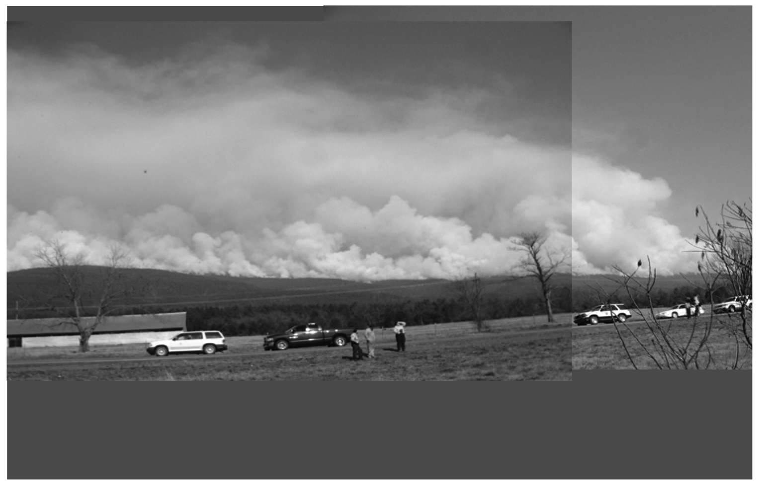
Regional scale air quality models require knowledge of how much smoke is discharged into the atmosphere as the plume rises to some maximum height. Plume rise ranges from hundreds of meters for prescribed fires to thousands of meters for wildfires. However, plume rise and dispersion from wildland fires is difficult to model because of complex plume dynamics. For example, Figure 1 shows the GOES satellite image of the plume produced by the 27 February 2004 Magazine Mountain, AR, prescribed burn (red area) at 1515 LST. The image, showing an expanding single plume transported towards northwestern Arkansas by the prevailing wind, gives an impression of being from a “scaled-up” version of an industrial plume. However, Figure 2 reveals a complex structure of merging multiple updraft “cores” when the plume is viewed from the ground.
Clearly the updraft structure of wildland fire plumes must be modeled correctly if accurate estimates for plume rise, amounts and heights of smoke injection in the atmosphere, and dispersion are to be made available for air quality models. Full-physics smoke plume models such as the active tracer high-resolution atmospheric model (ATHAM) [17,18] can model the complexity of wildland fire plume structures. Reference [19] simulated a prescribed burn in northwestern Washington which closely approximated measured elevations and concentrations of smoke. However, if the objective is to simulate hundreds of prescribed burns daily in the southern United States, much simpler modeling approaches would be required to make available plume rise data for operational air quality models such as CMAQ [16], its adaptive grid version [20] or WRF-Chem [21] for predicting air quality and assessing pollution control strategy development, exposure, impacts of regional climate change, and etc.
Reference [22] linked fuels information with meteorological data through VSMOKE, a Gaussian “screening” model for local smoke dispersion. VSMOKE attempted to account for plume complexity by placing 40% of smoke at the ground as an initial step. The Florida Fire Management Information System [23,24] merges the cross flow Gaussian horizontal dispersion properties of VSMOKE with three dimensional trajectories produced by HYSPLIT [25] to estimate smoke plume movement and the ground-level impact of PM2.5 concentrations on potentially hazardous visibility reductions.
This paper describes “Daysmoke”, an empirical-stochastic plume model designed to simulate multiple-core updraft smoke plumes from prescribed burns. Daysmoke is an extension of ASHFALL, a plume model developed to simulate deposition of ash from sugar cane fires [26]. As adapted for prescribed fire, Daysmoke consists of three models—an entraining turret model that calculates plume pathways, a particle trajectory model that simulates smoke transport through the plume pathways, and a meteorological “interface” model that links these models to weather data from high-resolution numerical weather models.
Model theory and assumptions are described in the next section. Results from validation studies for simulating weak plumes and applications to regional scale air quality modeling follow.
2. Model Theory and Description
Conceptually, a rising convective plume driven by heat from combustion entrains ambient air which adds to the plume mass while modulating its buoyancy and vertical velocity. Some plume air and particulate matter are detrained into the ambient air creating a “pall” of smoke extending downwind beneath the visible plume. The growing smoke plume ascends to near the top of the mixing layer. If the smoke plume is relatively weak (cool and slow-rising), all or part of it may be captured, torn apart, and dispersed by turbulence within the mixed layer before it rises to an altitude of thermal equilibrium. If the convective smoke plume is strong, most of the smoke may be ejected into the free atmosphere far above the top of the mixed layer with little or no smoke remaining to be dispersed within the mixed layer.
2.1. The Entraining Turret Model
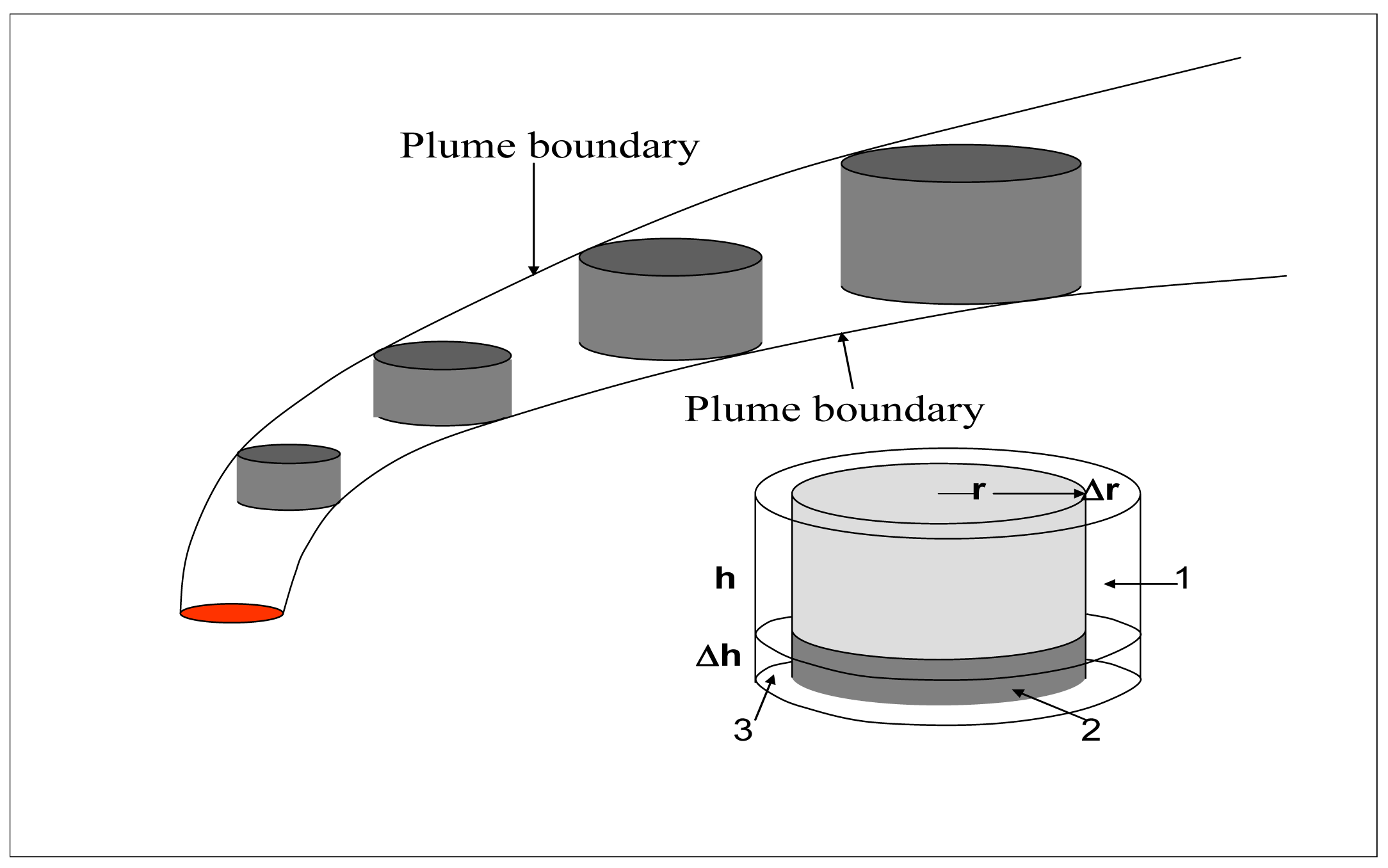
From photogrammetric analysis of video footage of smoke plumes from burning sugar cane, reference [27] determined that a rising smoke plume could be described by a train of rising turrets of heated air that sweep out a three-dimensional volume defined by plume boundaries on expanding through entrainment of surrounding air through the sides and bottoms as they ascend (Figure 3). The change in the volume (V) of radius (r) and height (h) of a rising turret by entrainment of ambient air as it passes from height z − 1 to z is,
Entrainment of heat and momentum (horizontal and vertical) is a function of the downwind tilt of the plume. For example, if the horizontal wind speed is zero (the plume rises vertically), all of the material entrained through the bottom and top of the turret is plume air while entrainment of ambient air takes place through the sides. As the plume tilts in the presence of wind, more ambient air is entrained through the bottom and top of the turret until, if the plume blows horizontally, all air entrained into the turret is ambient air.
Let Qe represent an ambient constituent, and Qz−1 represent the smoke plume constituent surrounding the turret at level z − 1. The constituent Qz at level z resulting from the mixing of the original turret with the entrained volume of mixed constituents is,
The derivation of the plume pathways is subject to two assumptions needed to make the problem tractable. First, changes in volume are equally distributed between deepening and expanding the turret. Second, the changes in volume will be functions of the rate of turret rise. Therefore,
Setting Q = T (temperature) in Equations (5) yields an equation for turret temperature for buoyancy calculations. Setting Q = (u, v, w) (any of the velocity components) yields an equation for plume drift. Setting Q = 1 yields an equation for the volume growth of the turret.
Initial conditions for plume temperature, rise rate, and volume start the plume rising through a veering/shearing horizontal wind field within a stratified atmosphere. Once the initial conditions are specified, Equation (5) is solved numerically to yield the plume pathway (Figure 3). In addition, the rise rate is adjusted for buoyancy through
Equation (5) does not include adiabatic expansion of the rising plume. For the vast majority of prescribed burns in the southeastern United States (for which plume tops are less than 2 km), scale analysis shows that omission of adiabatic expansion leads to errors in the calculation of plume expansion of less than 3%—an error far smaller than uncertainties in the measurement of fuel characteristics. However, should Daysmoke be used in modeling of large plumes from wildfires, the errors of omission of adiabatic expansion can become significant—perhaps as large as 30% for plumes growing above 10 km. Therefore adiabatic expansion is calculated from [29],
Moist processes activate a simple cloud parameterization in Daysmoke. A cumulus cloud forms when the moisture (mixing ratio) within a rising, entraining turret exceeds the saturation mixing ratio calculated for the turret temperature. Both turret temperature and mixing ratio are calculated via Equation (5). The entire turret is assumed to be saturated. All liquid water remains within the cloud. The cloud ascends by a weighted average of the dry and moist adiabatic lapse rates calculated for the rising turret at its temperature and pressure. The cloud top is the elevation where the cloud mixing ratio falls below the saturation mixing ratio at plume temperature and pressure. Though adequate for shallow cumulus clouds that may form over prescribed burn plumes, the cloud parameterization is not adequate for modeling deep, precipitating pyro-cumuli that form on occasion above intense wildfires.
In addition to ambient weather data, Equation (5) must be supplied with the entrainment coefficient (e) and initial values for the plume—effective plume diameter (D0 = 2r0), vertical velocity (w0), and the difference between plume and ambient temperatures (ΔT0). The effective plume diameter is defined as the diameter a plume would have if emissions from an irregular-shaped burning area were spread over a circular area.
Observations of plumes from large-perimeter prescribed fires reveal the presence of several updraft cores or subplumes. These updraft cores may vary in size depending on the type, loading, and distribution of various fuels. Multiple-core updraft plumes, being smaller in diameter than a single core updraft plume, would be more impacted by entrainment and thus would be expected to grow to lower altitudes. If the effective plume diameter and initial vertical velocity are replaced by initial volume flux,
Defining what constitutes updraft cores is complicated by the merging convective sub-plumes often observed with prescribed burns (Figure 2). Thus the multiple-core updraft capability of Daysmoke remains an oversimplification of complex plume structures from prescribed burns. It becomes convenient to assert that a particular plume “behaves as an n-core updraft plume” even though the number of observed updraft cores may differ from n.
The entrainment coefficient is calculated internally in Daysmoke. For calm air and neutral stratification, reference [28] found entrainment coefficients for vertical plumes from industrial stacks to range from 0.080 for “jets” (high momentum plumes of low buoyancy) to 0.155 for buoyant plumes. For bent-over plumes, Briggs reported entrainment coefficients in the range from 0.52 to 0.66. Thus, for the full range of buoyant plumes (from erect through bent-over), entrainment coefficients vary from 0.155 to 0.66. Let the entrainment coefficient be proportional to a plume “bent-overness” index B0 defined as
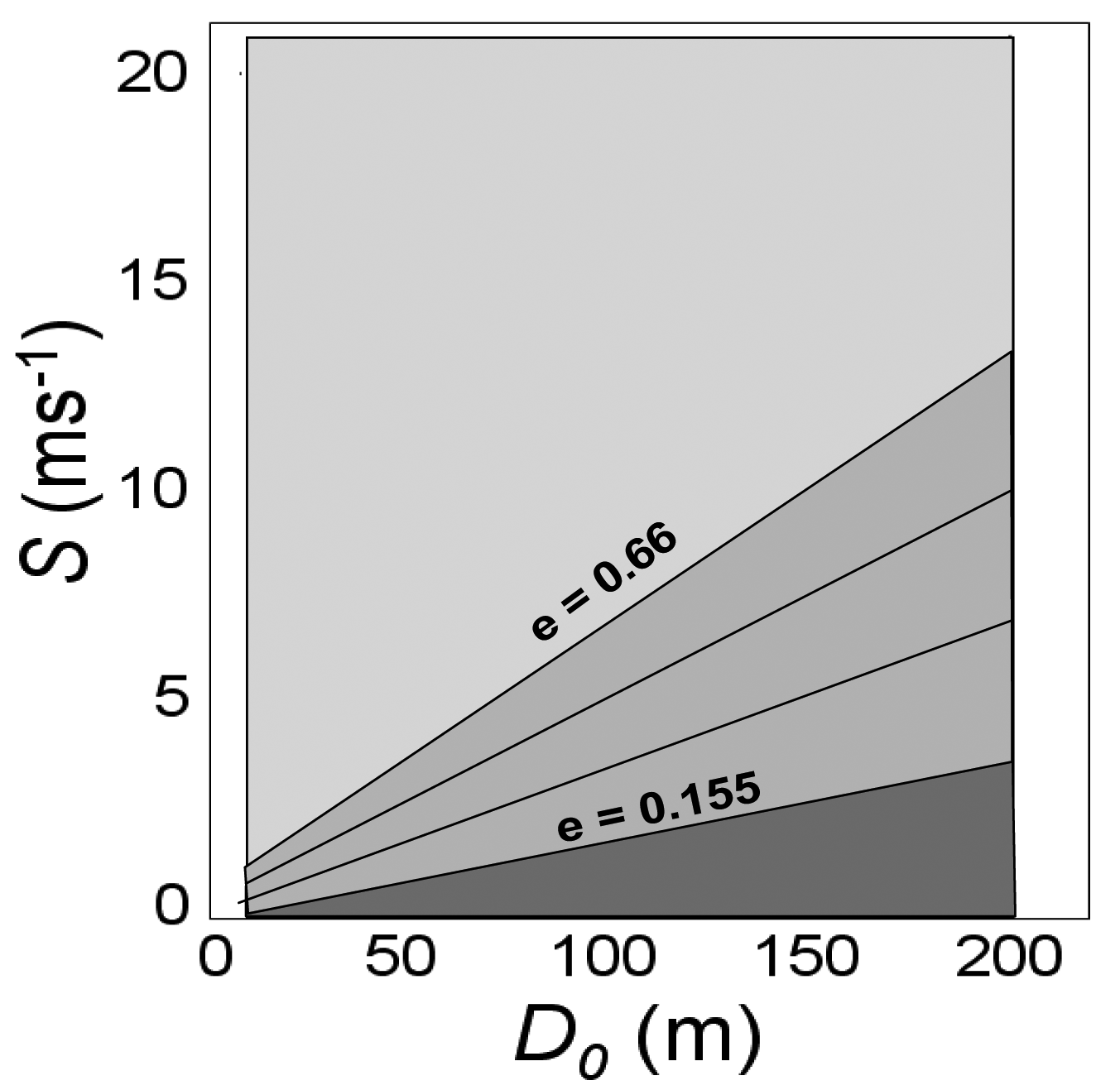
For prescribed burns, bent-overness can be represented as the ratio of the strength of the transport wind S with the strength of the plume as given by w0. However, w0 is fixed in Daysmoke and the strength of the plume is better represented by the effective plume diameter D0. Let the ratio Dm/Sm represent a scaling factor determined by the range of S (0 < S < 20 ms−1) and of D (0 < D < 200 m) for prescribed burns. The range of B0 is subject to the constraint that 0.155 < ek < 0.66. Thus ek becomes a dynamic variable that changes during the course of the day as the depth of the mixing layer and wind speeds change and during the course of the burn as plume conditions change.
Figure 4 maps entrainment coefficients for the ranges of transport wind speeds and initial plume diameters described above. Most of the area is assigned the maximum entrainment coefficient, ek = 0.66 (light gray area) meaning most prescribed burns fit the bent-over designation. However, for larger diameter burns and/or weak to moderate transport wind speeds, the entrainment coefficient is variable within the range defined by the medium gray area.
2.2. The Detraining Particle Model
Particles are released at the base of the multiple-core updraft plumes defined by the entraining turret module. Each particle represents a pre-assigned mass of smoke particulate matter. The particles ascend through each plume at the mean velocity components that define the three-dimensional wind speed for each level of the entraining turret module. The particles are spread laterally as the plume widens. At each time step there is added to these velocities a stochastic component that approximates turbulent spreading of smoke as it rises.
The location of a particle over an interval of time, Δt, as it traverses the plume volume is given by,
Each particle is tracked through the plume volume until it is discharged into the free atmosphere by either (1) detrainment across plume boundaries, (2) plume capture by convective circulations, or (3) discharge through the plume top when plume vertical velocity falls below a threshold vertical velocity wc.
2.3. The Meteorological Interface Model
The interface model can be of any design and complexity but, for operational considerations, it has been kept relatively simple. The interface model links Daysmoke with hourly vertical profiles of weather data taken from numerical weather prediction models. These data are hourly averages and do not represent high frequency processes that mix and disperse smoke within the boundary layer. Therefore the interface model includes a simple formulation for deep convective mixing.
After a particle is discharged from the plume, the change in its position is given by,
The formulation for convective circulations is described in Appendix A. A string of two-dimensional mass conservative sinusoidal circulation cells oriented normal to the mean wind vector within the mixing layer and with a translation speed equal to the mean wind vector describe the convective boundary layer. The cells are mutually independent—amplitude, phase, wavelength and time history may differ. The equations in Appendix A yield the convective velocity components (uce, vce, Wce) for each particle subject to knowledge of the reference rotor velocity, wr, for a mixing layer depth of 1 km.
3. Model Analysis (FAST Analysis and Comparison with Briggs Theory)
3.1. FAST Analysis
Table 1 lists coefficients, the range of values, the assigned values and the expected impacts on plume height (P. Hgt) and ground-level concentrations of particulate matter (GLC). The ranges of values have been determined through approximately 200 simulations to define “reasonable” facsimiles of prescribed fire smoke plumes.
The updraft core number n ranges between one and ten for prescribed burns typical of the southern United States. The updraft core number is specific to each burn and is critical for determining plume height and ground-level smoke concentration.
The small scale mixing coefficient cs is the only mechanism in Daysmoke for the horizontal spread (normal to the plume axis) of the smoke plume. The simulations determined that the small scale mixing coefficient must fall in the range 0 < cs < 1. There was no lateral plume spread with cs = 0. Simulations with cs = 1 spread the plume too broadly with ground-level smoke concentrations too low as compared with observed concentrations. A more realistic range for cs is 0.2 < cs < 0.5. Other factors of plume structure, such as the definition and persistence of convective eddies in vertical cross sections of smoke plumes simulated by Daysmoke, support the choice of cs = 0.3.
The threshold vertical velocity ranges between 0.1 < wc < 1.0 ms−1. It was found that vertical velocity profiles for strong plumes that penetrate into stable airmasses above the mixing height typically decline the final meter per second over a short distance—usually less then 20 m. Weak plumes that do not penetrate above the mixing height are broken up by turbulence and dispersed within the mixing layer. Thus the choice for wc for either strong or weak plumes has little impact on plume height or ground-level smoke concentrations.
The detraining particle module does require specification for two variables: terminal velocity wf and threshold vertical velocity wc. In Daysmoke, the terminal velocity is wf = −0.0002 ms−1. For the range of applications of Daysmoke, wf is negligible and has no impact on model calculations nor smoke sedimentation.
The expected range for the reference rotor velocity for a mixing layer of depth 1 km lies between 0.5 < wr 2.0 ms−1. Choosing wr too small reduces the rate smoke is transported from aloft to the ground thus yielding smoke concentrations that are too small relative to observations. Simulation results suggest wr = 1.0 ms−1.
Given assigned values for the coefficients in Table 1, only the updraft core number remains to be determined. Factors contributing to updraft core number include: size of the burn, shape of burn area, heterogeneity of fuels, fuel type, moisture, and loadings, distribution of fire on landscape, amount of fire on landscape, distribution of canopy gaps, transport wind speed, and mixing layer depth. The updraft core number is critical for modeling plume top height and ground-level smoke concentrations.
The relative impacts of these coefficients on plume height (second to the last column of Table 1) were assigned following a Fourier Amplitude Sensitivity Test (FAST) applied to a larger set of model coefficients (Table 2) derived from an earlier version of Daysmoke. (Note that the coefficient names in Table 2 do not necessarily correspond to the coefficient names in Table 1.)
The FAST analysis was introduced by [30] as a method to vary input variables simultaneously through their ranges of possible values following their given probability density functions (i.e., values which have a greater probability are chosen more often). All input parameters are assumed to be mutually independent and each is assigned a different frequency, which determines the number of times that the entire range of values is traversed. With each input parameter oscillating at a different characteristic frequency, a different set of input parameter values is obtained for each model run with every value used once. The mean and variance, which characterize the uncertainty due to the variability of the input parameters, are calculated for model output parameters. Fourier analysis of each output for all model runs is used to separate the response of the model to the oscillation of particular input parameters. Summation of those Fourier coefficients corresponding to a particular input parameter frequency and its harmonics determines the contribution of that input parameter to the model output variances. Finally, by scaling the relative contribution of the input parameters to the total variance, partial variances are obtained, which show the sensitivity of model output parameters to the variation of individual input parameters in terms of a percentage of the variance. The Fourier coefficients corresponding to input parameter frequencies and their harmonics do not account for the entire variance of the model outputs. The Fourier coefficients corresponding to linear combinations of more than one input parameter frequency account for the remaining fraction of the variance, which can be attributed to the combined influences of two or more parameters.
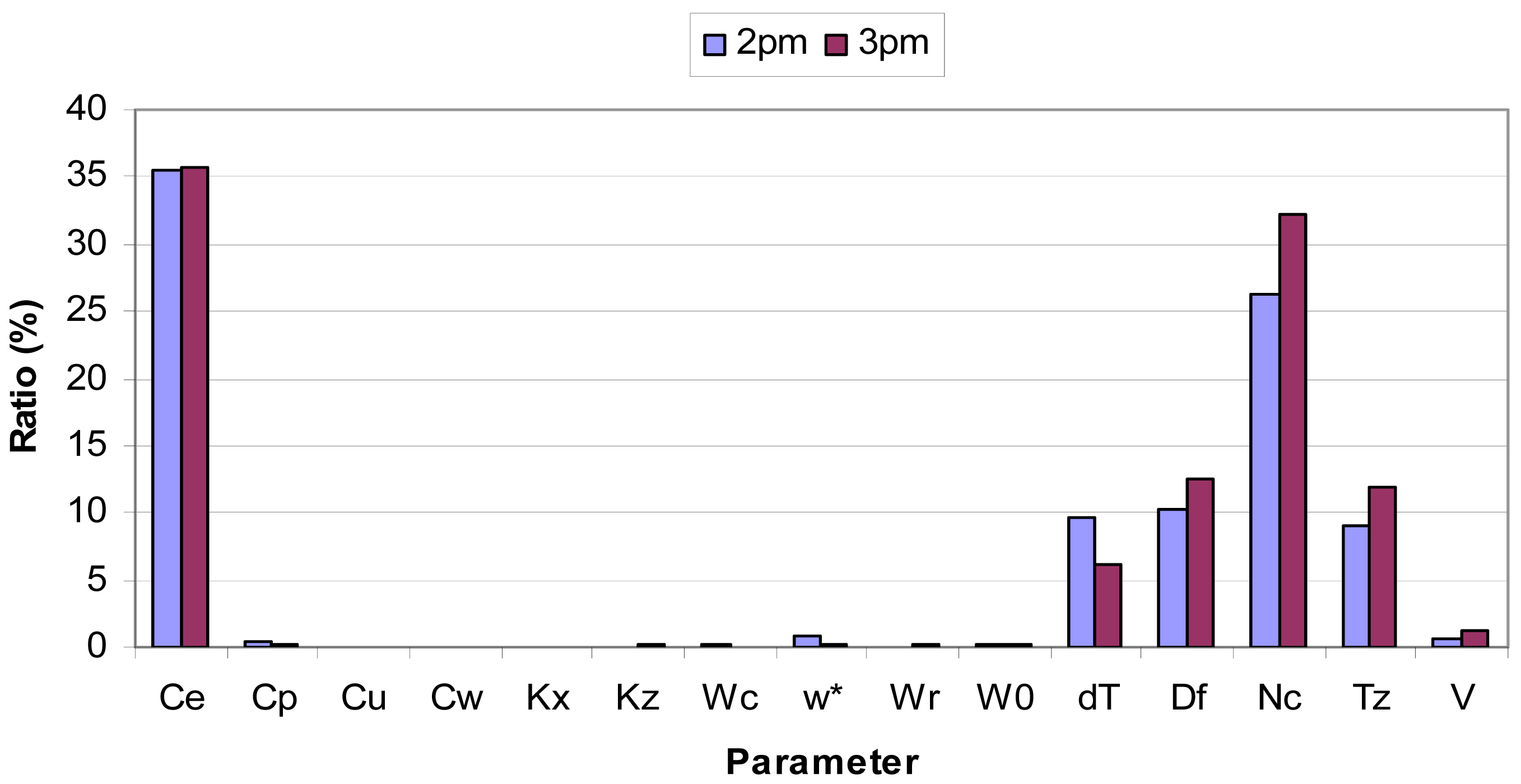
Details of the FAST analysis for a prescribed burn can be found in [10]. FAST results are shown in Figure 5. The ratio of partial variance of a parameter to total variance varies from one hour to another throughout the simulation period, but it only slightly affects the relative importance of this parameter to others. The results for two hours are shown to indicate this variation. The 15 parameters can be divided into three categories in terms of their importance. The first category includes the two most important parameters: the plume entrainment coefficient and number of plume updraft cores. Their ratios are about 35 and 26%, respectively, at 1400, and 35 and 32% at 1500. In other words, each parameter contributes one fourth to one third to the total variance. The second category includes three important parameters: the initial plume temperature anomaly, diameter of flaming area, and thermal stability. Their ratios are about 10% at 1400 and vary between 6 and 12% at 1500. Thus, each contribute about one tenth to total variance on average. The third category includes the remaining parameters, whose ratios are 1% or less. These parameters are not important to Daysmoke plume rise simulation.
The outcome of the FAST analysis was a redesign of Daysmoke with unimportant coefficients either pre-assigned or expressed in terms of other variables. The result is the reduced number of coefficients shown in Table 1.
3.2. Input Data
Initial and hourly weather data include vertical profiles of temperature, three-dimensional components of the wind, and moisture (mixing ratio) for a location representative of the meteorology in the vicinity of the prescribed burn.
As regards initial values for the plume—D0, w0, and ΔT0 fire activity data include fuel type/amount (currently determined by National Fire Danger Rating Sytem Fuel Model [31] the area burned, the location of the burn and the date/start time of the burn. In addition the Each firing technique: backing fire, strip-head fires, head fire, ring fire and aerial ignition [32] produces fires of differing intensity and spread rates.
The process of converting from this description of a prescribed burn to the required Daysmoke inputs proceeds in four basic steps: fuel consumption calculation, total emissions calculation, hourly emissions and determination of D0. The first three components are similar to those of the BlueSky Smoke Modeling Framework [33]. Total fuel consumption for each burn is determined using the single parameter regression equations for version 2.1 of CONSUME as given in appendix C of the User's Guide [34]. For each burn, total emissions for a number of chemical species are then calculated by multiplying the total consumed fuel by a species-specific emissions factor (Table 3). Values for the emissions factors are taken from the average emission factors of 26 intensively studied southeastern prescribed burns during 1995 and 1996 [35].
Hourly emissions are derived from this total value using the Emissions Production Model (EPM) [36] that derives time series of emissions and heat release for a fire based on a fairly simple source strength model. The time scale for completion of the flaming component is determined by the theoretical fire behavior. For a given wind speed, head/flanking/back fire spread rates are determined from BehavePlus [37] for the appropriate NFDRS fuel model.
The heat release rate (Q) is simply estimated as 50% of the product of the mass of fuel consumed per hour and the heat of combustion (1.85 × 10⁷ J kg−1) [38]. The assumed 50% reduction in the heat release rate is designed to restrict only a portion of the total heat released going into the plume with the other 50% going into the heating of surrounding vegetation and ground surface. The initial values for the plume—D0, w0, and ΔT0 can be related to the heat of the fire [39] by
Equation (15) with the above specified initial conditions is assumed to be valid at some reference height h0 defined as the base of the plume where flaming gasses and ambient air have been thoroughly mixed and where the incipient plume temperature ΔT0 of 40 °C is found. For small prescribed burns, h0 may be found approximately 10 m above ground and for wildfires, h0 may be found several 100's of meters above ground. For a typical grassfire [40] h0 can be found near 35 m.
The number of particles released per time step is determined from hourly emissions derived from the total fuel consumption [34] using the Emissions Production Model (EPM) of [36] modified for prescribed burns.
3.3. Comparison with Briggs and LES Model Plumes
Reference [41] used a high-resolution large eddy simulation (LES) model to explore the dynamics of buoyant plumes arising from a heat source representative of wildland fires. The model was designed to resolve the majority of the turbulent eddies in the plume and its environment, and thus does not suffer from approximations inherent in simple empirical plume models. Referenced [42] compared mean plume trajectories from the LES model with the two-thirds law plume rise model of [28] and its modification by [43] to account for finite-area sources. They found that within the first kilometer downwind from the heat source the mean plume rise seen in the simulations was well-described by the power law trajectory and is in reasonably good agreement with simple plume rise calculations. The LES and Briggs results place narrow bounds on mean plume trajectories and therefore provide a critical validation test for Daysmoke.
A version of the Briggs formulation provided by [44], and modified by [45] allows for insertion of the initial values used for Daysmoke.
Here,
x = the horizontal distance along the plume centerline downwind from the stack.
U = the mean horizontal wind speed (ms−1) for the air layer containing the plume.
ΔT0 = the plume temperature (K) anomaly.
w0 = the stack gas ejection speed (ms−1).
D0 = the internal exit diameter (m) of the stack.
H = the height of the plume axis above the source (stack) (m).
e = the entrainment coefficient (conventionally, 0.66) for the Briggs model.
g = gravitational acceleration (ms−2).
Te = plume exit temperature (K).
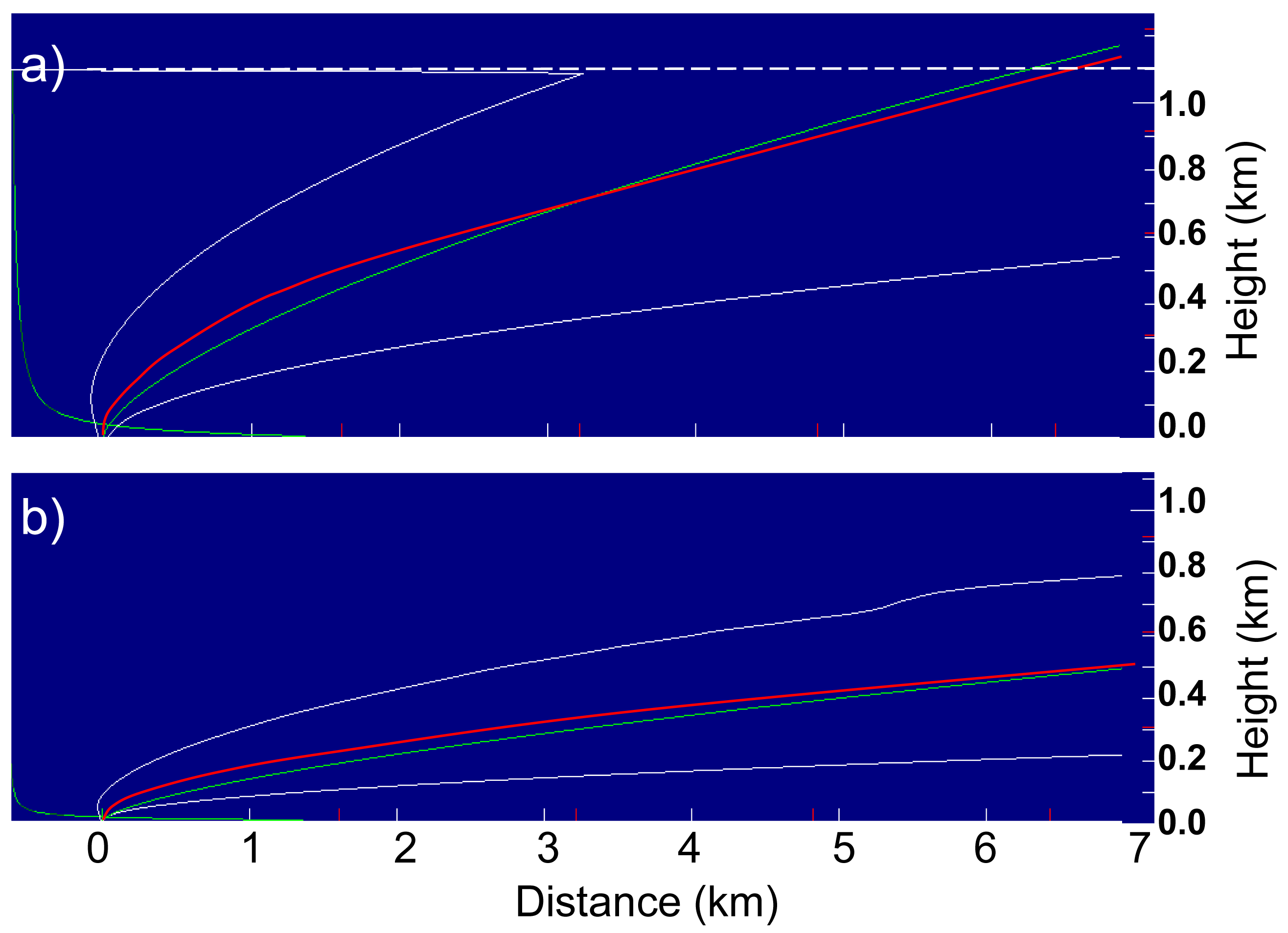
Daysmoke was run with a test profile of temperature and wind created from a WRF generated sounding for Ft. Benning, GA, for 23 January 2009. All winds below 1700 m were set to blow from the west with a speed of U = 9.0 ms−1 as the Briggs theory is set for a layer mean wind speed. The outcome of the comparison for the first seven kilometers downwind is shown in Figure 6. Plume boundaries calculated via Equation (5) are shown by the white lines. The green lines identify mean plume trajectories from the Briggs two-thirds law for a neutral atmosphere. For the initial effective plume diameter D0 = 62 m (Figure 6a), the Daysmoke plume, driven by the hyperbolic vertical velocity profile (alternating dark and light green lines at the left side of the figure), rose more steeply during the first 500 m downwind. Then the centerline for the Daysmoke plume declined from 60 m above the Briggs trajectory at 500 m downwind to intersecting the Briggs trajectory at 3.2 km downwind. The outcome was a more highly bent-over plume. Beyond 3.2 km, the Daysmoke centerline ran slightly below the Briggs trajectory—15 m below where the centerlines crossed the mixing height (dashed line) at 7.3 km downwind from the ignition site.
Similar results were found for the smaller D0 = 17.0 m plume (Figure 6b). This Daysmoke plume initially rose more steeply than the Briggs trajectory for the first 150 m downwind placing the plume approximately 25 m above the Briggs trajectory. Then the two curves gradually converged past 7.5 km downwind.
It is apparent that the Daysmoke plumes are initially more vigorous but, overall, the plume rise is well-explained by the power-law trajectory. The differences are minimal in comparison with the area swept out by the plume boundaries.
4. Model Evaluation (Study of Weak Plumes)
During 2008–2009, a smoke project was conducted at Fort Benning, GA. The site was chosen because of the large size of its prescribed burn operation and the aggressiveness of its burn program—typically a 1–3 year fire return interval. Burning when fuel loadings had increased to just carry fire would not be expected to release heat sufficient to loft a towering plume. Daysmoke simulations produced some plumes that ascended to the mixing height. Other simulated plumes rose partway through the mixing layer before losing identity as a plume—breaking up and being redistributed by convective circulations.
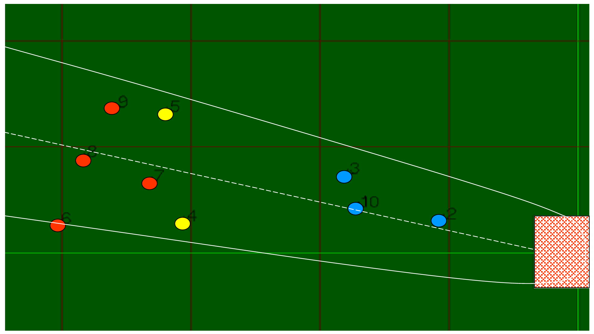
The project collected data on plume top height and ground-level PM2.5—both critical data sets for validation of Daysmoke—for eleven burns. Three mobile trucks, each equipped with pairs of DustTrak real-time PM2.5 samplers [46], were operated at distances of roughly 1 mile, 2 miles, and 4 miles downwind from the burn. The trucks were moved when wind shifts created the necessity to relocate beneath the smoke plumes. An example of the truck protocol is shown in Figure 7. The three trucks (color coded) were moved to various positions during the burn to maintain location under the plume (shown schematically by the parabolic boundaries) as judged by the truck crews. PM2.5 observations by the DustTrak samplers were corrected for wood smoke by multiplying by a factor of 0.275.
Daysmoke was run with hourly vertical profiles of wind, humidity, and temperature from high-resolution weather simulations by the WRF model. Emissions data were provided by the methodology described in c) Input Data above.
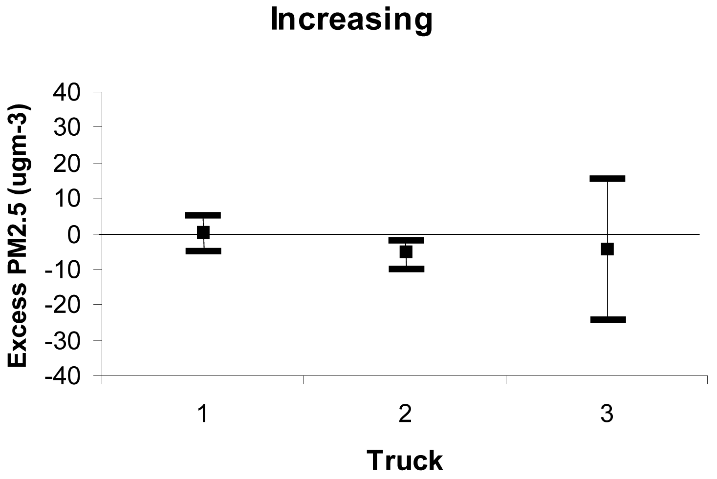
Our analysis placed the eleven burns in five categories (Table 4). The first column shows that three burns fell into the first category-ground-level smoke concentrations increased with distance from the burn. Plume statistics are summarized in Figure 8. Daysmoke contains stochastic terms for convective circulations that are set so they cannot be repeated. Thus successive Daysmoke runs will give slightly different answers. To smooth out the effects of the stochastic terms, we constructed ensemble averages of five simulations. The averages of the residuals (defined as the differences between ensemble averages and observed PM2.5) for the periods of the burns (defined as time of ignition until completion of ignition) for the three days are shown by the squares in Figure 8. The spreads of residuals are given by the horizontal bars connected by the vertical lines. Average residuals for all three trucks ranged less than ± 5 μgm−3. The magnitudes of the spreads for Truck1 and Truck 2 never exceeded 10 μgm−3. Given uncertainties in defining updraft core number and model errors in wind speed and direction, the results for the first category of Table 4 are as good as can be expected from an empirical-statistical modellike Daysmoke.
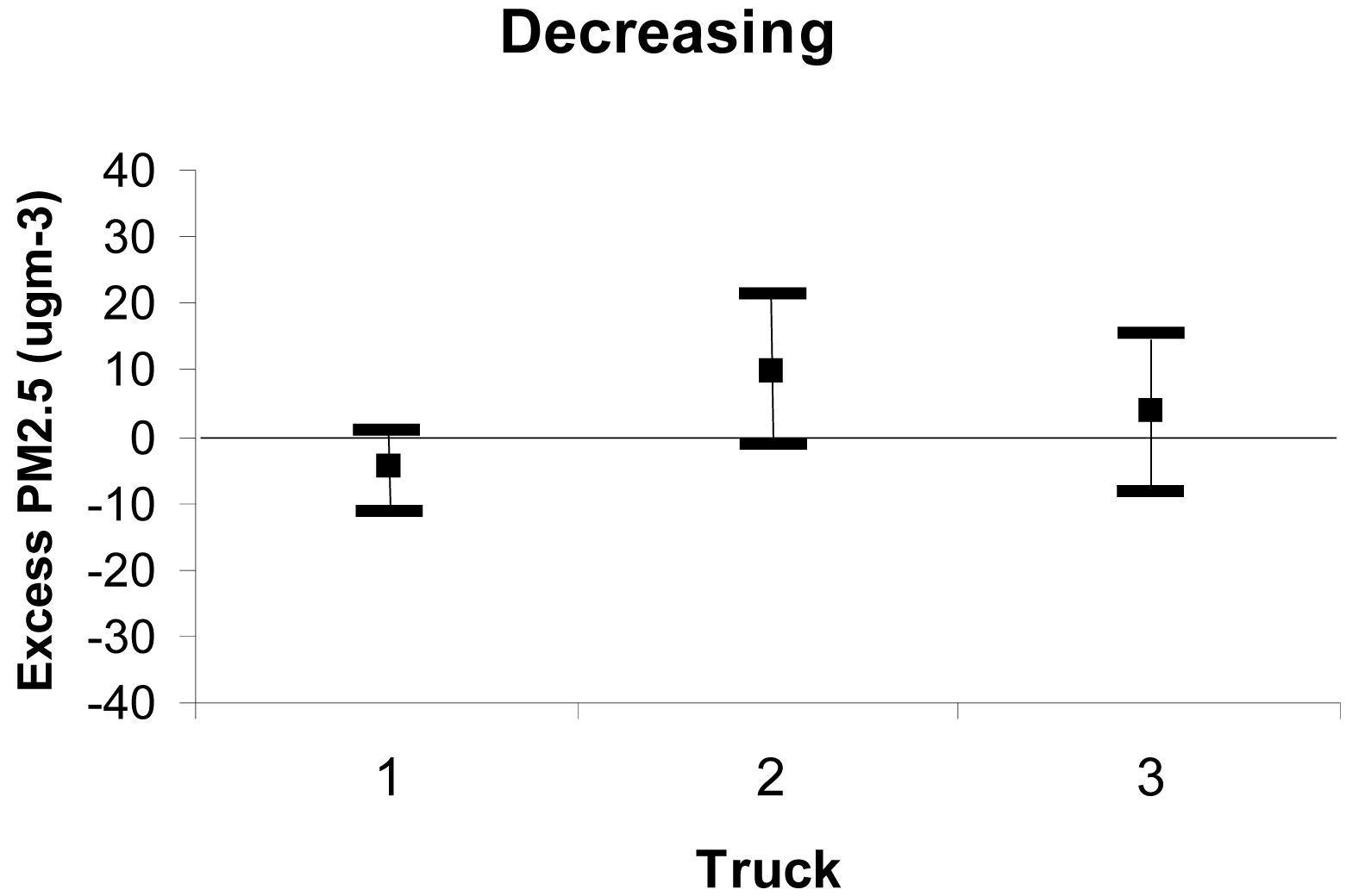
The results for the second category of Table 4—ground-level smoke concentrations decreased with distance from the burn - are shown in Figure 9. Daysmoke slightly under-predicted smoke at Truck 1 and over-predicted smoke at Truck 2 and Truck 3. The discrepancies are small—less than 10 μgm−3. Spreads also were small at all three trucks; the larges being 21 μgm−3.
The third column of Table 4 lists the two days with plumes characterized by very high concentrations of smoke at Truck 1 and very steep gradients of smoke concentration between the trucks (Figure 10). Daysmoke greatly under-predicted burn event smoke at Truck 1—minus 60 μgm−3 with a spread ranging from −32 to −89 μgm−3. The average residual was improved for Truck 2 (−12 μgm−3) but the spread remained high (−47 to 22 μgm−3). The better results at Truck 3 could be explained by the truck being located near the edges of the plumes.
The fourth and fifth columns of Table 4 list those days characterized by, respectively, truck locations away from the plume (either no roads or movement restricted by military activities) and corrupted or lost data.
The poor results from Daysmoke for the events characterized by high smoke concentrations at Truck 1 and steep gradients of PM2.5 between the trucks (column 3 of Table 4) needs further explanation. That these two events were extraordinary is shown by peak 30-s PM2.5 for the seven days for which complete data are available for all three trucks (Figure 11). Peak PM2.5 exceeding 600 μgm−3 for 15 January and 23 January 2009 imply that Truck 1 was located within the ascending plume on both days while Truck 2 and Truck 3 were located within particulate matter detrained from the plume as it passed overhead. This implication contrasts with Daysmoke solutions for the other days that placed the trucks either within detrained smoke or within remnants of the smoke plume torn apart and down-mixed by convective circulations.
Given the initial conditions of w0 = 25 m s−1 and ΔT0= 40 °C, no choice for updraft core number could produce both the very high smoke concentrations at Truck 1 nor the steep gradients of PM2.5 between the other trucks. Therefore the Daysmoke bent-over plume solution failed to reproduce the events of 15 January and 23 January 2009.
We varied the initial conditions subject to the constraint that the flux, given by the product of the initial velocity with the square of the initial effective plume diameter, was held constant. The top panel of Figure 12 shows the bent-over solution for a 1-core updraft plume for 23 January 2009. We reduced the initial conditions to w0 = 0.5 ms−1 and ΔT0 = 1.0 °C to obtain the solution for a “highly tilted” plume (middle panel of Figure 12). Conservation of total flux required increasing the initial effective plume diameter from 59 m to 417 m—a requirement that decreases the impact of entrainment on the plume. Thus the weakly buoyant highly-tilted plume was driven almost entirely by buoyancy and was capable of growth through the depth of the mixing layer.
The plume axis is characteristically quasi-linear as compared with the parabolic axis of the bent-over plume (upper panel). Running Daysmoke with the updraft core number set to eight (estimated for this burn) yielded the highly tilted plume solution shown in the lower panel of Figure 12. Note how this plume runs along the ground before ascending. The plume tilt of 15 degrees is greater than that for the 1-core plume (middle panel) and the plume is confined to the mixing layer. The red bars in Figure 10 show that the 30-min averaged PM2.5 difference between Daysmoke and observed smoke concentration at Truck 1 of −8 μgm−3 was greatly improved over the −89 μgm−3 calculated for the bent-over plume. Results for Truck 2 and Truck 3 showed minor changes from the original differences for 23 January 2009.
Is the highly-tilted plume represented by Briggs theory? Figure 13 shows plume boundaries (white lines) for the 1-core updraft 23 January 2009 simulation (aspect ratio: Δx/Δz = 2). The plume axis (red line) describes a plume that runs along the ground for approximately 0.6 km then rises at approximate 3.5 ms−1 (dark green/light green line) along a quasi-linear axis. The weak buoyancy of the plume, shielded from entrainment by its 417 m diameter, ascended to the mixing height 2 km downwind and rose 100 m above the mixing layer (light blue line). The Briggs solution (Equation 16), shown by the green line, has the plume ascending to 250 m 4 km downwind from the burn.
Is there independent evidence to support the Daysmoke solution for the highly-tilted plume? Figure 13 shows stack and cooling tower plumes from an electric power generating station. The stack plume shows the strongly bent-over parabolic structure (red line) typical of relative high velocity effluents rapidly slowed by entrainment on ejection through a relatively small plume diameter. The cooling tower plume, tilted along a linear axis (blue line), is characteristic of low velocity effluents ejected within a relative large plume diameter and driven by buoyancy. The plume structures modeled with Daysmoke compare favorably with the plumes shown in Figure 14.
Plume top heights (squares) and height ranges (connecting lines) for plumes simulated by Daysmoke (red squares in Figure 15) compare favorably with plume top heights measured by ceilometer (black squares). Relative to the observed lower range, Daysmoke plume tops were on the average 8 m high. However, relative to the observed higher range, Daysmoke tops were on the average −200 m low. Thus Daysmoke plume tops were, overall, slightly low.
5. Model Application (CMAQ)
An adaptive grid version of CMAQ (AG-CMAQ) has been recently developed to better resolve the processes involving plumes [20] AG-CMAQ integrates the adaptive grid algorithm of reference [47] into CMAQ version 4.5 and is based on the adaptive grid air pollution model described in [11,12]. AG-CMAQ employs r-refinement: the number of grid cells remains constant but grid nodes are moved to cluster in areas where plumes are detected. Although the nodes are relocated, their connectivity does not change and the structure of the grid is maintained. In AG-CMAQ, a curvilinear coordinate system is fitted to the adapted non-uniform grid and, using coordinate transformations, the governing equations are transformed to a space where the grid is uniform. Then the transformed equations are solved in this space by directly applying the CMAQ solution algorithms that are designed for uniform grids. A variable time-step algorithm [48] allows each cell in AG-CMAQ to be assigned a unique local time-step and was included in the model to improve computational efficiency.
The objective of grid adaptation in AG-CMAQ is to achieve more accurate representations of spatial fields by increasing grid resolution at locations where the error in numerical solutions is largest. The adaptation is achieved by estimating a weight function that efficiently quantifies numerical error and clustering grid nodes within the regions that result in the highest weights. The initial application of AG-CMAQ attempted to model biomass burning plumes impacting air quality in the Atlanta metropolitan area [20]. For that simulation, the Laplacian of the concentration of primary particulate matter from biomass burning was used as a weight function. Comparison of AG-CMAQ's performance to that of the static grid CMAQ model indicated that grid adaptation resulted in reduced numerical diffusion, better defined plumes, and closer agreement with site measurements. Here, we describe an application of AG-CMAQ to model prescribed burn plumes at Fort Benning, GA using information provided by Daysmoke.
Daysmoke can be applied as an emissions injector for AG-CMAQ in the same manner as it has been previously used with CMAQ. Detailed information describing plume rise or vertical distribution of buoyant prescribed burn emissions is necessary to achieve realistic results with gridded photochemical models that typically lack the mechanisms necessary to simulate this process. The fire emissions are injected into CMAQ's vertical layers following the vertical pollutant profile produced by Daysmoke at a downwind distance that allows full plume development. The location at which the emissions are injected within the horizontal CMAQ domain is not a straightforward choice. Injecting the emissions at the fire emissions source implies that a vertical profile modeled downwind of the fire is applied further upwind at the location of initial release. On the other hand, injection of emissions downwind at the location where the plume's fully developed vertical profile was estimated with Daysmoke entails neglecting chemistry and aerosol processes included in CMAQ but absent from Daysmoke up to this downwind distance. The error from either choice is greater as the downwind distance necessary to achieve a fully developed vertical plume profile increases relative to grid resolution. Plumes that rapidly reach their maximum plume rise and vertically distribute pollutants may not bring forth significant errors. However, given that full plume development may occur at distances larger than 15 km and grid resolution in CMAQ has been previously taken down to 1 km, this might not necessarily be the case. The significance of this issue is even greater in AG-CMAQ, where an initial increase in resolution around the source of emissions is meant to enhance chemical and physical processes shortly after release. In the future, a tighter coupling of Daysmoke with AG-CMAQ should address these issues.
In the following application we have modeled the effects on air quality from a prescribed burn at Fort Benning, GA on 9 April 2008. During this day, 300 acres of wildland were treated. Ignition occurred at 16:30 GMT and flaming continued until 18:45 GMT, with smoldering emissions continuing thereafter. This episode is of particular interest because peaking PM2.5 concentrations were recorded at the Columbus, GA airport air quality monitoring site, possibly due to the impact of the burn, providing an opportunity to compare modeled results to those observed at a regulatory network station.
Hourly emissions from the prescribed burn were estimated with the Fire Emission Production Simulator (FEPS) [49] using information provided by land managers at the site. Background emissions for the photochemical simulations were prepared using the Sparse Matrix Operator Kernel Emissions model (SMOKE, version 2.4) [50] with a 2002 “typical year” emissions inventory [51] projected to year 2008 using the existing control factors and the growth factors generated from the Economic Growth Analysis System (EGAS) Version 4.0. Meteorological data is provided through the Weather Research and Forecasting model (WRF, version 3.1) [52] at 1.333 km resolution and 34 vertical layers of increasing depth from the surface to the top. Initialization, boundary conditions constraining, and nudging at 6-hour intervals were performed using analysis products from the North American Mesoscale (NAM) model. The CMAQ domain covered 120 × 124 km over southwestern Georgia and southeastern Alabama with a 1.333 km horizontal grid spacing and 34 vertical layers.
Daysmoke simulations were undertaken using 6-updraft cores. For fire emissions injection into CMAQ we used the vertical plume profile estimated by Daysmoke 4 km downwind of the fire, and applied it at the location of the fire in the CMAQ domain. This length provided sufficient time for full plume development and was not exceedingly distant from the source (3 grid cells downwind). The time it takes the plume to reach a downwind distance of 4 km (3 × 1.33 km cells) varies with altitude and time, but for the majority of emissions in this particular fire, it takes about 15 minutes. During this time, some particles are discharged from the plume through the cited mechanisms. With slower wind speeds more particles are detrained, fall out, or get removed by convective eddies to be dispersed throughout the mixing layer.
The vertical distribution of PM2.5 fire emissions for the entire episode is shown in Figure 16. Note that the lower layers are thinner than are the higher layers and the distribution is not normalized. The maximum vertical injection height of fire emissions is at about 1 km (the 10th layer of the model). The WRF-simulated hourly mixing heights at the burning location during the flaming period (1100–1400 LST) were 753, 979, 1213 and 1334 meters, respectively. An additional 24 vertical layers extended the top of the CMAQ model domain to near 18 km.
The largest fraction of emissions is injected into layer 8, which spans an altitude from approximately 500 m to 680 m above the ground. Nearly 70% of fire emissions were distributed into layers 6, 7, and 8 which extend from approximately 335 m to 680 m above the ground. The same procedure was applied for fire emissions injection in the AG-CMAQ simulation. Grid adaptation was driven by the curvature in the fire emitted PM2.5 concentration field.
Figure 17 shows the time evolution of PM2.5 concentration at the Columbus Airport monitoring site 30 km from the location of the prescribed burn for both the CMAQ and AG-CMAQ runs, as well as available observational data. CMAQ overestimates the peak concentration while AG-CMAQ underestimates this value. However, the magnitude of the error in the maximum PM2.5 level for both models is approximately the same (4 μgm−3). A sharp increase in concentration is perceived in the observations after 21:00 UTC. Similarly, rapid increments are perceived in the CMAQ and AG-CMAQ simulations, although occurring at earlier times. The CMAQ-modeled PM2.5 concentrations fall abruptly after peaking, while the decrease is gentler with AG-CMAQ and more closely resembles that seen in the observations. Throughout the simulation, the mean fractional error in the modeled results relative to station observations was reduced by 17% on average using AG-CMAQ compared to CMAQ. A timing mismatch in observed and modeled peak pollutant levels is also evident. The fact that emissions estimated by FEPS are hourly starting at the top of the hour and ignition actually occurred 30 minutes past 16:00 GMT may at least partially account for the discrepancy.
Better understanding of the modeled results can be gained from the pollutant concentration fields shown in Figure 18. These pollutant fields correspond to the instance of maximum concentration at the Columbus airport location. The static grid CMAQ plume appears more diffused, relative to that produced with AG-CMAQ. It is also apparent that impact at the airport site is not direct, but rather a tangential hit. The pollutant field from the AG-CMAQ simulation shows a more concentrated plume with higher pollutant levels near a core that has persisted longer into the simulation. Significant grid refinement occurs at the source of emissions as well as along the plume centerline. The area surrounding the airport site also experiences appreciable refinement throughout the run. Figure 19 further contrasts the plumes produced with CMAQ and AG-CMAQ. These three-dimensional PM2.5 concentration plots show surface level concentrations as well as a 3D plume volume defined as a constant concentration surface for concentrations larger than 30 μgm−3. The viewer position has been rotated to better appreciate the plume volumes. From the images is it noticeable that the plume produced in the AG-CMAQ simulation offers a greater level of detail and is likely able to pick up finer details of the wind field to which it is subjected. The plume structures, undoubtedly, are highly dependent on the vertical pollutant distribution information provided by Daysmoke.
6. Summary and Concluding Remarks
In this paper we have presented the plume rise and dispersion model Daysmoke, intended for the simulation of smoke plumes from wildland fires. The model theory presented in this paper is the outcome of a former version that was subjected to a sensitivity analysis with the Fourier Amplitude Sensitivity Test (FAST). The FAST analysis identified empirical parameters important for plume height prediction. Therefore, many empirical coefficients have been pre-assigned or expressed in terms of other variables.
We compared Daysmoke plumes with Briggs theory and found good agreement for “bent-over” plumes although the two-thirds theory is not explicit in Daysmoke. However, the solutions for “highly-tilted” plumes characterized by weak buoyancy, low initial vertical velocity, and large initial plume diameter do not match Briggs theory.
We further evaluated Daysmoke by comparing simulations and observations of PM2.5 and plume height for weak plumes from eleven prescribed burns at Fort Benning, GA. Simulations of ground-level PM2.5 compared favorably with observations taken from three mobile trucks out to a distance of eight kilometers. Daysmoke plume tops were found near the lower end of the range of observed plume tops for six prescribed burns.
Daysmoke simulated vertical smoke profiles necessary for initializing the smoke concentrations in CMAQ (with and without adaptive grid). CMAQ simulation results show the detail and accuracy that can be obtained at the regional scale.
The initial plume vertical velocity of 25 ms−1 was assumed based on numerical simulations of coupled fire-atmosphere models [39] The vertical velocity was claimed to be an average over a 20 m grid square and representative of wildfires. However, plume diameters for the burns at Fort Benning, GA, were typically 60 m and the use of 25 ms−1 as an average initial vertical velocity for a 60 m diameter prescribed burn plume should be considered as problematic. In addition, canopy drag can further reduce the exit velocity. Forest canopies at Fort Benning ranged from open to partially closed. Positioning of field personnel away from the burns did not allow for observations. However, observations of trees rocking during plume passage at other prescribed burns are suggestive of significant momentum transfer from the plume to the crown. Furthermore, widespread crown scorch in the aftermath of prescribed burns is suggestive of significant heat transport from plume to trees. Thus the expected impact of canopies on an incipient plume would be to lower the initial vertical velocity and to reduce the initial temperature anomaly below those used for this study.
However, it is the mass flux determined by combustion equations that must be conserved. Reducing the initial average vertical velocity through canopy drag must necessarily be accompanied by a commensurate increase in initial plume diameter. That, in addition to reducing initial plume temperature anomaly through heat transfer to the crown, can lead to results that are counterintuitive because of the increased buoyancy efficiency of the larger diameter plume. For example, in this study (Figure 12), we reduced initial vertical velocity and initial plume temperature anomaly from, respectively, 25 ms−1 and 40 K for a 59 m diameter bent-over plume, to 0.5 ms−1 and 1.0 K for a highly-tilted plume and found the latter grew taller through an initial plume diameter seven times larger.
Thus the impact of the forest canopy may be to convert an incipient small diameter, fast-rising bent-over plume into a large diameter slow-rising highly-tilted plume capable of ascending farther than its bent-over counterpart. That Daysmoke plume heights scored slightly low in comparison with observations (refer to the discussion in reference to Figure 15) may in part be explained by our initialization for bent-over plumes. Further research will clarify this issue.
Finally, analyses just beginning of smoke observations of “strong plumes” from 55 prescribed burns should reveal the extent to which smoke from southern prescribed burns done by mass ignition penetrates above the mixing layer. In these events, a fraction of smoke emissions may not be available for dispersion locally downwind thus lowering threats to air quality below those predicted. However, smoke trapped within the free atmosphere above the mixing layer may be transported at different wind directions and speeds to be reintroduced into the mixing layer at unexpected locations.


| Constant | Definition | Range of Value | Assgn Value | Impact P Hgt. | GLC |
|---|---|---|---|---|---|
| n (none) | updraft core number | 1–10 | user input | major | major |
| cs (ms−1) | lateral plume spread | 0.2–0.5 | 0.30 | none | major |
| wc (ms−1) | threshold velocity | 0.1–1.0 | 0.3 | none | none |
| wf (ms−1) | particle terminal velocity | –––– | 0.0002 | none | none |
| wr (ms−1) | max rotor velocity | 0.5–2.0 | 1.0 | none | major |
| Model | Parameter | Meaning | Average | Range | Unit |
|---|---|---|---|---|---|
| ETM | Ce | Entrainment coefficient | 0.18 | 0.1∼0.5 | − |
| DPM | Cp | Plume detrainment coefficient | 0.03 | 0.01∼0.2 | − |
| Cu | Air horizontal turbulence coefficient | 0.15 | 0.1∼0.2 | − | |
| Cw | Air vertical turbulence coefficient | 0.01 | 0.01∼0.1 | − | |
| Kx | Thermal horizontal mixing rate | 1 | 1∼1.5 | km(m/s)/°C | |
| Kz | Thermal vertical mixing rate | 1 | 1∼1.5 | km(m/s)/°C | |
| Wc | Plume-to-environment cutoff velocity | 0.5 | 0.2∼0.8 | m/s | |
| w* | Air induced particle downdraft velocity | 0.01 | 0.01∼0.02 | m/s | |
| Wr | Large eddy reference vertical velocity | 1 | 1∼1.5 | m/s | |
| W0 | Initial plume vertical velocity | Computed | 5∼15 | m/s | |
| ΔT0 | Initial plume temperature anomaly | Computed | 5∼15 | °C | |
| Df | Effective diameter of flaming area | Computed | −25∼25% | m | |
| Nc | Number of updraft core | 1 | 1∼20 | (−) | |
| Tz | Atmospheric thermal lapse rate | Observed | −25∼25% | °C/km | |
| V | Average wind speed | Observed | −25∼25% | m/s |
| Chemical Species | Emission Factor (g/kg) | |
|---|---|---|
| Flaming Combustion | Smoldering Combustion | |
| CO2 | 1664.00 | 1649.00 |
| CO | 82.00 | 106.00 |
| CH4 | 2.32 | 3.42 |
| C2H4 | 1.30 | 1.30 |
| C2H2 | 0.50 | 0.48 |
| C2H6 | 0.32 | 0.46 |
| C3H6 | 0.51 | 0.59 |
| C3H8 | 0.09 | 0.11 |
| C3H4 | 0.05 | 0.05 |
| NMHC | 2.77 | 3.00 |
| PM2.5 | 11.51 | 10.45 |
| Increase | Decrease | Extreme Decrease | Out of Plume | Misc |
|---|---|---|---|---|
| 3 | 3 | 2 | 2 | 1 |
| 9 April 08 | 14 April 08 | 15 January 09 | 13 January 09 | 14 January 09 |
| 21 January 09 | 15 April 08 | 23 January 09 | 20 January 09 | |
| 8 April 09 |
Acknowledgments
The study is funded in part of the Southern Regional Models for Predicting Smoke Movement Project (01.SRS.A.5) funded by the USDA Forest Service National Fire Plan, the Joint Fire Sciences Program of the USDA and Department of Interior (JFSP 081606 and JFSP 081604), the Department of Energy-Savannah River Operations Office through the USDA Forest Service Savannah River under Interagency Agreement DE-AI09-00SR22188, the National Research Initiative Air Quality Program of the Cooperative State Research, Education, and Extension Service U.S. Department of Agriculture, (Agreement No. 2004-05240), and the U.S. Department of Defense through the Strategic Environmental Research and Development Program (SERDP-RC-1647).
7. Appendix A
A string of two-dimensional mass conservative sinusoidal circulation cells oriented normal to the mean wind vector within the mixing layer and with a translation speed equal to the mean wind vector describe the convective boundary layer. The cells are mutually independent—velocity amplitude, phase, wavelength and time history may differ. The equations for convective circulations at each particle location (x, y, z) are:
The variable, wr (ms−1), is the reference rotor velocity for convective eddies if the mixing layer depth is 1 km; h (m) is the depth of the mixing layer; um, vm, and S are, respectively, the mean u-component and mean v-component for the mixing layer, and the transport wind speed. C is a shape factor, here set to 1.0 so that the convective eddies will have equal horizontal and vertical dimensions. The constants, c1, c2, and c3 are amplitude weights: c1 = 1200 sets the lifetime of a convective eddy to 20 minutes, c2 = 2117 and c3 = 23 multiplies Cn (a set of 10 randomly selected numbers that range from 0–9). Many choices for c2 and c3 are possible. The selections are made so that adjacent eddy cells will have different time and amplitude histories.
References
- SRFRR. Southern Region Forest Research Report, 7th American Forest Congress; U.S. Department of Agriculture: Forest Service, Southern Research Station, Ashville, NC, USA; February; 1996. [Google Scholar]
- Stanturf, J.A.; Wade, D.D.; Waldrop, T.A.; Kennard, D.K.; Achtemeier, G.L. Fires in southern forest landscapes. In The Southern Forest Resource Assessment; Wear, D.M., Greis, J., Eds.; Gen. Tech. Rep. SRS-53; U.S. Department of Agriculture: Forest Service, Washington, DC, USA, 2002; pp. 607–630. [Google Scholar]
- Wade, D.D.; Brock, B.L.; Brose, P.H.; Grace, J.B.; Hoch, G.A.; Patterson, W.A., III. Fire in eastern ecosystems. In Wildland Fire in Ecosystems: Effects of Fire on Flora; Brown, J.K., Smith, J.K., Eds.; Gen. Tech. Rep. RMRS-42; U.S. Department of Agriculture, Forest Service, Rocky Mountain Research Station: Ogden, UT, USA, 2000; Volume 2, pp. 53–96. [Google Scholar]
- Achtemeier, G.L. Effects of moisture released during forest burning on fog formation and implications for visibility. J. Appl. Meteorol. Climatol. 2008, 47, 1287–1296. [Google Scholar]
- Achtemeier, G.L. On the formation and persistence of superfog in woodland smoke. Meteorol. Appl. 2009, 16, 215–225. [Google Scholar]
- Naeher, L.P.; Achtemeier, G.L.; Glitzenstein, J.S.; MacIntosh, D.; Streng, D.R. Real-time and time-integrated PM2.5 and CO from prescribed burns in chipped and non-chipped plots—Firefighter and community exposure and health implications. J. Exposure Sci. Environ. Epidemiol. 2006, 16, 351–361. [Google Scholar]
- Zheng, M.; Cass, G.R.; Schauer, J.J.; Edgerton, E.S. Source apportionment of PM2.5 in the Southeastern United States using solvent-extractable organic compounds as tracers. Environ. Sci. Technol. 2002, 56, 2361–2371. [Google Scholar]
- Liu, Y.-Q.; Achtemeier, G.L.; Goodrick, S. Sensitivity of air quality simulation to smoke plume rise. J. Appl. Remote Sens. 2008, 2, 1–12. [Google Scholar]
- Liu, Y.-Q.; Goodrick, S.; Achtemeier, G.L.; Jackson, W.A.; Qu, J.J.; Wang, W. Smoke incursions into urban areas: Simulation of a Georgia prescribed burn. Int. J. Wildland Fire 2009, 18, 336–348. [Google Scholar]
- Liu, Y.-Q.; Achtemeier, G.L.; Goodrick, S.; Jackson, W.A. Important parameters for smoke plume rise simulation with Daysmoke. Atmos. Poll. Res. 2010, 1, 250–259. [Google Scholar]
- Odman, M.T.; Khan, M.N.; McRae, D.S. Adaptive Grids in Air Pollution Modeling: Towards and Operational Model. In Air Pollution Modeling and its Application XIV, 1st ed.; Gryning, S.E., Schiermeier, F.A., Eds.; Kluwer Academic/Plenum Publishers: New York, NY, USA, 2001; pp. 541–549. [Google Scholar]
- Odman, M.T.; Khan, M.N.; Srivastava, R.K.; McRae, D.S. Initial Application of the Adaptive Grid Air Pollution Model. In Air Pollution Modeling and its Application XV, 1st ed.; Borrego, C., Schayes, G., Eds.; Kluwer Academic/Plenum Publishers: New York, NY, USA, 2002; pp. 319–328. [Google Scholar]
- Lee, S.; Russell, A.G.; Baumann, K. Source apportionment of fine particulate matter in the southeastern United States. J. Air Waste Manag. Assoc. 2007, 57, 1123–1135. [Google Scholar]
- Hu, Y.M.; Odman, T.; Chang, M.E.; Jackson, W.; Lee, S.; Edgerton, E.S.; Baumann, K. Simulation of air quality impacts from prescribed fires on an urban area. Environ. Sci. Technol. 2008, 42, 3676–3682. [Google Scholar]
- Byun, D.W.; Ching, J. Science Algorithms of the EPA Model-3 Community Multiscale Air Quality (CMAQ) Modeling System; National Exposure Research Laboratory: Research Triangle Park, NC, USA, 1999. [Google Scholar]
- Byun, D.W.; Schere, K.L. Review of the governing equations, computational algorithms, and other components of the Models-3 Community Multiscale Air Quality (CMAQ) modeling system. Appl. Mech. Rev. 2006, 59, 51–77. [Google Scholar]
- Herzog, M.; Graf, H.-F.; Textor, C.; Oberhuber, J.M. The effect of phase changes of water on the development of volcanic plumes. J. Volcanol. Geotherm. Res. 1998, 87, 55–74. [Google Scholar]
- Oberhuber, J.M.; Herzog, M.; Graf, H.-F.; Schwanke, K. Volcanic plume simulation on large scales. J. Volcanol. Geotherm. Res. 1998, 87, 29–53. [Google Scholar]
- Trentmann, J.; Andreae, M.O.; Graf, H.-F.; Hobbs, P.V.; Ottmar, R.D.; Trautmann, T. Simulation of a biomass-burning plume: Comparison of model results with observations. J. Geophys. Res. 2002, 107, 1–15. [Google Scholar]
- Garcia-Menendez, F.; Yano, A.; Hu, Y.; Odman, M.T. An adaptive grid version of CMAQ for improving the resolution of plumes. Atmos. Poll. Res. 2010, 1, 239–249. [Google Scholar]
- Grell, G.A.; Peckham, S.E.; Schmitz, R.; McKeen, S.A.; Wilczak, J.; Eder, B. Fully coupled online chemistry within the WRF model. Atmos. Environ. 2005, 39, 6957–6975. [Google Scholar]
- Lavdas, L.G. Program VSMOKE–Users Manual.; USDA Forest Service General Technical Report SRS-6; U.S. Department of Agriculture: Forest Service, Southern Region: Ashville, NC, USA, 1996; p. 147. [Google Scholar]
- Goodrick, S.L.; Brenner, J. Florida's Fire Management Information System. University of Idaho Press: Boise, ID, USA, 1999; 1, pp. 3–12. Available online: http://jfsp.nifc.gov/conferenceproc/Goodricketal.pdf accessed on 12 March 2009). [Google Scholar]
- Brenner, J.; Goodrick, S.L. Florida's Fire Management Information System. Proceedings of EastFire Conference; George Mason University: Fairfax, VA, USA, May 2005; pp. 11–13. [Google Scholar]
- Draxler, R.R.; Hess, G.D. Description of the Hysplit 4 Modeling System; NOAA Technical Memorandum ERL ARL-224: Washington, DC, USA; December; 1997. [Google Scholar]
- Achtemeier, G.L. Predicting dispersion and deposition of ash from burning cane. Sugar Cane 1998, 1, 17–22. [Google Scholar]
- Achtemeier, G.L.; Adkins, C.W. Ash and smoke plumes produced from burning sugar cane. Sugar Cane 1997, 2, 16–21. [Google Scholar]
- Briggs, G.A. Plume Rise Predictions. In Lectures on Air Pollution and Environmental Impact Analyses; American Meteorological Society: Boston, MA, USA, 1975; pp. 72–73. [Google Scholar]
- Hess, S.L. Introduction to Theoretical Meteorology; Henry Holt & Co.: New York, NY, USA, 1959. [Google Scholar]
- Cukier, R.I.; Fortuin, C.M.; Shuler, K.E.; Petschek, A.G.; Schaibly, J.H. Study of the sensitivity of coupled reaction systems to uncertainties in rate coefficients. I. Theory J. Chem. Phys. 1973, 59, 3873–3878. [Google Scholar]
- Deeming, J.E.; Lawrence, J.W.; Fosberg, M.A.; Furman, R.W.; Schroeder, M.J. National Fire Danger Rating System; Rocky Mountain Forest and Range Experiment Station Research Paper RM-84; U.S. Department of Agriculture: Forest Service, Fort Collins, CO, USA, 1972. [Google Scholar]
- Wade, D.D.; Lunsford, J.D. A Guide for Prescribed Fire in Southern Forests. In The Managed Slash Pine Ecosystem, 1st ed.; Stone, E.L., Ed.; School of Forest Resources and Conservation, University of Florida: Gainesville, FL, USA, 1983. [Google Scholar]
- O'Neill, S.M.; Ferguson, S.A.; Peterson, J.; Wilson, R. The BlueSky Smoke Modeling Framework. Proceedings of the 5th Symposium on Fire and Forest Meteorology, 16–20 November 2003; American Meteorological Society: Orlando, FL, USA.
- Ottmar, R.D.; Anderson, G.K.; DeHerrera, P.J.; Reinhardt, T.E. Consume Version 2.1 User's Guide; Department of Agriculture: Forest Service, Pacific Northwest Research Station, Portland, OR, USA, 1999. Available online: http://www.fs.fed.us/pnw/fera/products/consume/CONSUME21_USER_GUIDE.DOC (accessed on 19 July 2009).
- Hao, W.M. Personal communication; 2002. [Google Scholar]
- Sandberg, D.V.; Peterson, J. A Source Strength Model for Prescribed Fire in Coniferous Logging Slash. Proceeding of 1984 Annual Meeting of the Air Pollution Control Association, Pacific Northwest Section, Portland, OR, USA; 1984. [Google Scholar]
- Andrews, P.L.; Bevins, C.D.; Seli, R.C. BehavePlus Fire Modeling System, Version 3.0: User's Guide.; Gen. Tech. Rep. RMRS-GTR-106WWW Revised; U.S. Department of Agriculture: Forest Service, Rocky Mountain Research Station: Ogden, UT, USA, 2005. [Google Scholar]
- Byram, G.M. Combustion of forest fuels. In Forest Fire control and Use; Davis, K.P., Ed.; McGraw Hill: New York, NY, USA; pp. 155–182.
- Mercer, G.N.; Weber, R.O. Fire Plumes in Forest Fires: Behavioral and Ecological Effects; Johnson, E.A., Miyanishi, K., Eds.; Academic Press: New York, NY, USA, 2001; pp. 225–256. [Google Scholar]
- Jenkins, M.A.; Clark, T.; Coen, J. Coupling Atmospheric and Fire Models. In Forest Fires: Behavior and Ecological Effects; Johnson, E.A., Miyanishi, K., Eds.; Academic Press: San Diego, CA, USA, 2001; pp. 258–301. [Google Scholar]
- Clements, C.B.; Zhong, S.; Goodrick, S.; Li, J.; Potter, B.E.; Bian, X.; Heilman, W.E.; Charney, J.J.; Perna, R.; Jang, M.; et al. Observing the dynamics of wildland grass fires: FireFlux—A field validation experiment. Bull. Am. Meteorol. Soc. 2007, 88, 1369–1382. [Google Scholar]
- Cunningham, P.; Goodrick, S.L.; Hussaini, M.Y.; Linn, R.R. Coherent vertical structures in numerical simulations of buoyant plumes from wildland fires. Int. J. Wildland Fire 2005, 14, 61–75. [Google Scholar]
- Cunningham, P.; Goodrick, S.L. High-resolution numerical models for smoke transport in plumes from wildland fires. In Remote Sensing and Modeling Applications to Wildland Fires; Qu, J.J., Riebau, A., Yang, R., Sommers, W., Eds.; Springer Publishing: New York, NY, USA, 2011; pp. 74–88. [Google Scholar]
- Mills, M.T. Modeling the release and dispersion of toxic combustion products from pool fires. Proceedings International Conference on Vapor Cloud Modeling, Cambridge, MA, USA; 1987. [Google Scholar]
- Stern, A.C. Air Pollution Volume I; Academic Press: NewYork, NY, USA, 1968; p. 51. [Google Scholar]
- Fisher, B.E.A.; Metcalfe, E.; Vince, I.; Yates, A. Modelling plume rise and dispersion from pool fires. Atmos. Environ. 2001, 35, 2101–2110. [Google Scholar]
- Liu, S. Downwind Real-Time PM2.5 and CO Monitoring during Prescribed Forest Burns at Fort Benning GA. Master's Thesis, University of Georgia, Athens, GA, USA, 2010. [Google Scholar]
- Srivastava, R.K.; McRae, D.S.; Odman, M.T. An adaptive grid algorithm for air-quality modeling. J. Comput. Phys. 2000, 165, 437–472. [Google Scholar]
- Odman, M.T.; Hu, Y. A variable time-step algorithm for air quality models. Atmos. Polution Res. 2010, 1, 229–238. [Google Scholar]
- Anderson, G.; Sandberg, D.; Norheim, R. Fire Emission Production Simulator (FEPS) User's Guide Version 1.0; Department of Agriculture: Forest Service: Washington, DC, USA, 2004. [Google Scholar]
- CEP. Sparse Matrix Operator Kernel Emissions Modeling System (SMOKE) User Manual; Carolina Environmental Program: Chapel Hill, NC, USA, 2003. [Google Scholar]
- MACTEC. Documentation of the Revised 2002 Base Year, Revised 2018, and Initial 2009 Emission Inventories for VISTAS; Visibility Improvement State and Tribal Association of the Southeast (VISTAS): Ashville, NC, USA, 2005. [Google Scholar]
- Michalakes, J.; Dudhia, J.; Gill, D.; Henderson, T.; Klemp, J.; Skamarock, W.; Wang, W. The Weather Research and Forecast Model: Software Architecture and Performance. Proceedings of the Eleventh ECMWF Workshop on the Use of High Performance Computing in Meteorology; Zwieflhofer, W., Mozdzynski, G., Eds.; World Scientific: Singapore, 2005; pp. 156–168. [Google Scholar]
© 2011 by the authors; licensee MDPI, Basel, Switzerland. This article is an open access article distributed under the terms and conditions of the Creative Commons Attribution license (http://creativecommons.org/licenses/by/3.0/).
Share and Cite
Achtemeier, G.L.; Goodrick, S.A.; Liu, Y.; Garcia-Menendez, F.; Hu, Y.; Odman, M.T. Modeling Smoke Plume-Rise and Dispersion from Southern United States Prescribed Burns with Daysmoke. Atmosphere 2011, 2, 358-388. https://doi.org/10.3390/atmos2030358
Achtemeier GL, Goodrick SA, Liu Y, Garcia-Menendez F, Hu Y, Odman MT. Modeling Smoke Plume-Rise and Dispersion from Southern United States Prescribed Burns with Daysmoke. Atmosphere. 2011; 2(3):358-388. https://doi.org/10.3390/atmos2030358
Chicago/Turabian StyleAchtemeier, Gary L., Scott A. Goodrick, Yongqiang Liu, Fernando Garcia-Menendez, Yongtao Hu, and Mehmet Talat Odman. 2011. "Modeling Smoke Plume-Rise and Dispersion from Southern United States Prescribed Burns with Daysmoke" Atmosphere 2, no. 3: 358-388. https://doi.org/10.3390/atmos2030358