Radar-Based Analysis of Convective Storms over Northwestern Italy

Abstract

Thunderstorms may cause large damages to infrastructures and population, therefore the possible identification of the areas with the highest occurrence of these events is especially relevant. Nevertheless, few extensive studies of these phenomena with high spatial and temporal resolution have been carried out in the Alps and none of them includes North-western Italy. To analyze thunderstorm events, the data of the meteorological radar network of the regional meteorological service of Piedmont region (ARPA Piemonte) have been used in this work. The database analyzed includes all thunderstorms occurred during the warm months (April to September) of a 6-year period (2005–2010). The tracks of each storm have been evaluated using a storm tracking algorithm. Several characteristics of the storms have been analyzed, such as the duration, the spatial and the temporal distribution, the direction and the distance travelled. Obtained results revealed several important characteristics that may be useful for nowcasting purposes providing a first attempt of radar-based climatology in the considered region.

1. Introduction

Quantitative understanding of the spatial and temporal distribution of thunderstorms may provide a useful tool to define the most vulnerable areas and to improve the forecasting of such events. Many climatological studies about intense convective precipitation have been conducted to understand which geographical areas are prone to floods or damages caused by heavy rainfall [1,2].

These studies were accomplished using surface station reports which normally describe the thunderstorm tracks [1,3,4]. Most recently, the adoption of data provided by weather radars often combined with those of other meteorological networks (e.g., surface stations, lightning detection systems) produced more detailed and reliable results. In addition to ground rainfall, observations derived by weather radars enable the retrieval of many parameters as the vertical structure of precipitation, the ice particle distribution in clouds or the spatial coverage of the precipitation event. Furthermore, radar observations are usually available with a temporal resolution of ten minutes or higher.

Although many studies to investigate thunderstorms properties were performed in many regions of the United States (e.g., [2,5,6]), only a few were carried out in Europe [7,8,9].

The objective of this study is to identify the principal characteristics of thunderstorms over North-western Italy and to build a preliminary climatology of storm events in order to provide a statistical support for operational nowcasting activities. To this end, data from the two polarimetric C-band radars managed by Arpa Piemonte [10] have been used. Six years of data from 2005 to 2010 have been considered for the analysis. Even though the relatively short duration of the period is not sufficient for a complete climatological analysis, it can be considered adequate to detect the main features of local convective storms.

In order to identify convective cells, a storm identification and tracking algorithm has been employed. The storm tracking algorithm detects convective events with a maximum reflectivity larger than a given threshold and tracks them in space and time. Once the database including all the storm tracks have been created, the behavior of convective cells in the region has been analyzed to assess specific relations among the most relevant parameters of the storms. In addition, the local scale characteristics has been investigated in order to detect specific spatial patterns linked to the orography of the region. Finally, the thunderstorms location and motion have been compared with the mid-tropospheric winds deduced by radiosounding measurements.

The paper is organized as it follows: in Section 2 the radar network and the dataset characteristics, the storm tracking methodology and the post-processing operations are presented. In Section 3 the main climatological features of thunderstorms, their spatial and temporal distribution and their relation with tropospheric winds are discussed. Finally, in Section 4 the conclusions are drawn.

2. Data and Method

This study is based on the data collected by the operational radar network managed by Arpa Piemonte. The radar network is composed of two polarimetric C-band radars: the Bric della Croce radar (Bric hereafter), placed at 736 m a.s.l. on the top of the Torino hill and the Monte Settepani radar (Settepani hereafter), placed at 1386 m a.s.l. on the Apennines, at the border between Piemonte and Liguria regions. Arpa Piemonte also manages a third radar, a transportable X-band system, but since this system is not operational (it is used instead for specific measurement campaigns) it is not considered in this work. Main technical characteristics of the C-band systems are listed in

Table 1. Bric della Croce and Monte Settepani radar system specifications.

	Bric Della Croce	Monte Settepani
Radar type	Meteor 400C (Gematronik)	GPM 250C (Selex)
Polarization type	Simultaneous H and V	Alternate H and V
Antenna type	Central feed	Central feed
Antenna diameter	4.2 m	4.2 m
Beam width	1.0 deg max. w/o radome	1.0 deg max. w/o radome
Maximum sidelobe level	−28 dB	−28 dB
Maximum cross polar discrimination	−25 dB	−25 dB
Antenna gain	44.5 dB	44.5 dB
Radome type	Sandwich	Sandwich
Radome transmission loss	0.2 dB max., one way	0.2 dB max., one way
Transmitter type	Magnetron	Klystron
Frequency	5640 MHz	5625 MHz
Peak Power	250 kW	250 kW
Pulse length	0.5, 2.0 µs	0.5, 1.5, 3.0 µs
PRF	300–1200 Hz	300–1200 Hz
Range resolution	340 m (4 averaged samples)	375 m (5 averaged samples)

, while radars’ position is displayed in Figure 1a. The operational volume coverage pattern consists of a scan at 170 km range for the Bric radar (136 km for Settepani radar) with a set of 11 elevations (−0.1° to 28.5° for Bric, 0.3° to 28.5° for Settepani) and transmitting a short pulse (0.5 µs). Settepani also performs a secondary volume scan for qualitative monitoring at 250 km (3.0 µs pulse) with only three low elevations. The whole schedule is repeated every 10 min for both radars. Periodic six-monthly preventive maintenance is performed by the manufacturer on both radars. Electronic measurements during the maintenance tasks ensure that the radar constant is carefully checked and accurate within approximately 1 dB. In addition, an operational inter-calibration of the two radars is performed on a daily basis, when enough meteorological echoes are available in the overlapping region, by comparing the 3D volume scan intersecting bins. This check provides a useful way to detect eventual drift of one’s radar calibration.

The data considered for this study refer to the 6-year period 2005–2010. Due to the specific interest in convective precipitation, only the warm months from April to September have been considered. Both radars have dual-polarization capabilities since the beginning of the period analysed, i.e., in addition to horizontal reflectivity (Z_h), Doppler Velocity (V) and spectral width (σV ) they were able to measure the differential reflectivity Z_dr . Hardware upgrades performed afterwards increased the set of polarimetric parameters available. Specifically, during the summer of 2005 the Settepani signal processor was upgraded to measure differential propagation phase shift Φ_dp and correlation coefficient ρ_HV . The Bric radar had the same receiver upgrade in May 2008. At the same time a power splitter replaced the ferrite polar switch and the receiver was moved from the bottom of the radar tower to the antenna (mounted behind the dish). This involved a change from alternate transmission of orthogonal polarizations to simultaneous transmission. The Settepani radar, on the other hand, still uses alternate transmission. The change in the available polarimetric parameters (and the way they are calculated) during the period considered makes a statistical analysis extremely challenging. It was therefore decided to not consider the dual-polarization measurements for the storm characterization in this instance, but to focus instead on the horizontal reflectivity measurements only. The polarimetric information was however heavily exploited in the data quality control process, specifically for the clutter identification described in the following section. In a future work K_dp (the specific differential phase shift, i.e., the range derivative of Φ_dp) will be considered to extend the present reflectivity-based storm analysis. In fact K_dp has the remarkable advantages of being immune to calibration errors and to be closely related to the rainfall rate [11].

2.1. Fuzzy Logic Algorithm for Clutter Identification

The algorithm for clutter identification, mainly based on the work of [12], is operationally implemented on both C-band radars. An asymmetric beta distribution is used as the form of the radar and temperature membership functions (MBF), to allow more flexibility in shaping the probability density:

(1)

where the parameters m, a_l, a_r, b_l, b_r are derived for each hydrometeor and radar parameter, based on electromagnetic scattering models and statistical analysis over samples of known hydrometeor type [13]. With respect to [12] here the inference rule is not the product of all the MBF: the total probability (P_T ) for each hydrometeor type is given by the product of the temperature MBF and the weighted sum of the MBF of radar parameters Z_h, Z_dr , K_dp (specific differential phase shift, i.e., the range derivative of Φ_dp) and ρ_HV :

(2)

where N = 4, x₁ = Z_h, x₂ = Z_dr , x₃ = K_dp, x₄ = ρ_HV , w(x_i) are the weights associated with each radar parameter and T is the temperature from either sounding or model. The different treatment of temperature and radar variables is motivated by the need to mitigate the effect of measurement errors, especially on the dual-polarization parameters, which may show unreliable values mainly due to partial beam filling, side lobes effects, low signal to noise ratio. With the aim to decrease the measurement noise, all radar variables are averaged over a 3 beams × 3 range gates window in the polar volume. When the total probability is below 0.5, the radar cell is considered not classified. The hydrometeor classes are: large drops, drizzle, rain, heavy rain, hail mixed with rain, hail, graupel, wet snow, dry snow, crystals. A peculiarity of this implementation is that the clutter is treated exactly as an additional hydrometeor type and is identified within the same fuzzy logic volume processing, allowing a reduced total computation time. In this case five additional radar parameters are considered: ρ_HV , spatial variance of Z_dr , spatial variance of Φ_dp, Doppler velocity, difference between the actual and a statistical clear sky reflectivity map. When the total probability for the clutter class (Equation (2)) is above 0.5, the polar bin is flagged as contaminated, irrespective of the probability associated to the other meteorological classes. Out of the fuzzy scheme, further checks on the vertical gradient of reflectivity are performed to identify eventual anomalous propagation and second trip echoes. Figure 2 shows an example of a maximum reflectivity map for a convective event before and after the clutter removal process.

2.2. Composite of Lowest Level Reflectivity

Once the polar volume of reflectivity is flagged for clutter, a lowest level Cartesian map is derived for every radar. Initially a 2D polar map is computed, considering the first elevation free of orographic blocking at every (azimuth, range) location. The orographic blocking is estimated using the optical visibility calculated form a high resolution (50 m) digital elevation model. Subsequently the 2D polar map of lowest level reflectivity is transformed in Cartesian coordinates using a simple and fast nearest neighbor assignment. The geographical reference system for the Cartesian products is UTM ED50 (Universal Transverse Mercator, European Datum 1950). The coordinates of the radar maps are conventionally named utmX and utmY (distance along the x and y-directions in km within the fuse 32, covering North-Western Italy). The individual radar maps are then merged to form a radar composite for the North-Western Italy. Different criteria could be used in the merging process (mean, maximum, weighted mean, etc.). The operational procedure implements a weighted average for the merging, the weights being inversely proportional to the height of the radar beam above the ground (estimated from the same optical visibility maps used for the individual radar). The current Cartesian resolution of the radar composite is 0.8 km × 0.8 km. The dBZ reflectivity values are stored in the composite map, leaving to subsequent processing the conversion to rainfall intensity.

2.3. Processing for Cell Tracking

In order to characterize thunderstorms, cell parameters derived by the storm tracking algorithm operationally used in ARPA Piemonte since 2005 have been considered. Convective cells are identified analyzing relative maximum values of surface rainfall estimated by the radar composite [14]. To define a convective cell, all grid points on the composite map exceeding 40 dBZ are detected. Afterwards, all grid points exceeding 35 dBZ surrounding the relative maximum already detected are associated to it: a minimum of 5 grid points on the radar domain (which is about 3 km² at the current radar resolution) must be identified, otherwise the cell is discarded. In this way, for each cell a centroid is defined.

Once active cells are localized, several meaningful storm parameters are computed and associated to the centroid: they can be derived by other composite products, as storm top, storm vertical-integrated- liquid [VIL, 15] or associated probability of hail, or derived by satellite data as cloud top and cloud temperature. Tracking is performed in two steps. At first all possible children of a certain parent reflectivity core are searched using the well-known COTREC technique [16,17].

In order to increase the reliability of the assignments, some constraints (derived from previous analysis) are applied to reduce the number of possible children: the maximum distance between parent and child reflectivity core is fixed at 8 km, the speed associated with the child core must be less than 3 times the parent one, and finally the new cell cannot reverse the direction of propagation with respect to the previous tracked ones (i.e., the maximum angle is fixed at 180°). Thereafter the assignments are reduced to more probable ones. In this way, all active convective cores within the observation area of the Arpa Piemonte radar systems are identified and tracked, providing storm information about the maximum reflectivity, the duration, the area covered by the convective cell, the travelled distance and other meaningful parameters.

In order to exclude from the analysis possible artifacts and to have a sufficiently uniform database across the whole radar composite domain, the following post-processing operations were performed:

• all cells for which no tracking is available were excluded;
• to produce a reliable dataset, the region of the study was limited. Two criteria were used: (1) a radius of 150 km from the radar locations was imposed in order to consider only events occurred inside this circular area, mitigating the impact of beam broadening; (2) only regions characterized by good radar visibility, i.e., where the height of the lowest non-occluded beam is lower than 5000 m a.s.l., were considered. This second restriction was introduced to allow the detection of thunderstorms with relatively small vertical development.

The resulting area, extended for about 71,500 km² and hereafter referred as target area (Figure 1), includes almost the whole Liguria and Piemonte region. Two small exceptions are the far end of Val di Susa (Western sector) and Val d’Ossola (Northern sector). However, the target area extends in some territories of France (W), Val d’Aosta (NW), Lombardy (E) and Emilia-Romagna (SE) regions, as well as in the Ligurian Sea. The total number of tracks considered over the target area in the 6-year period analyzed is 36,253.

In the following sections several statistics over the cell tracks are presented. Since the reflectivity of the storm cells is in general roughly normally distributed in logarithmic units (dBZ), the statistics (mean, standard deviation, etc.) are calculated over the dBZ values, although this is not a physical unit. The median value may have also been considered, with very similar results, but due to the quantization error (reflectivity is recorded in 8-bit data, giving a 0.5 dB resolution), the arithmetic mean of the log values was finally preferred. This has the advantage of getting a more representative description of the actual distribution of the observations, compared to averaging the backscattered power (the linear reflectivity in mm⁶m⁻³), whose distribution is highly positively skewed. The logarithmic mean is always closer to the median values (generally within 1 dB), compared to the linear mean which may differ from the median by several dB. Mean values of reflectivity are expressed in dBZ while differences are expressed in dB, being non-dimensional quantities corresponding to ratios in linear units.

3. Results

3.1. The Storm Lifecycle

All storm tracks were classified according to their duration (see

Table 2. Number of thunderstorms tracked in function of their duration.

Duration (min)	20	30	40	50	60	70	80	90	100	>100
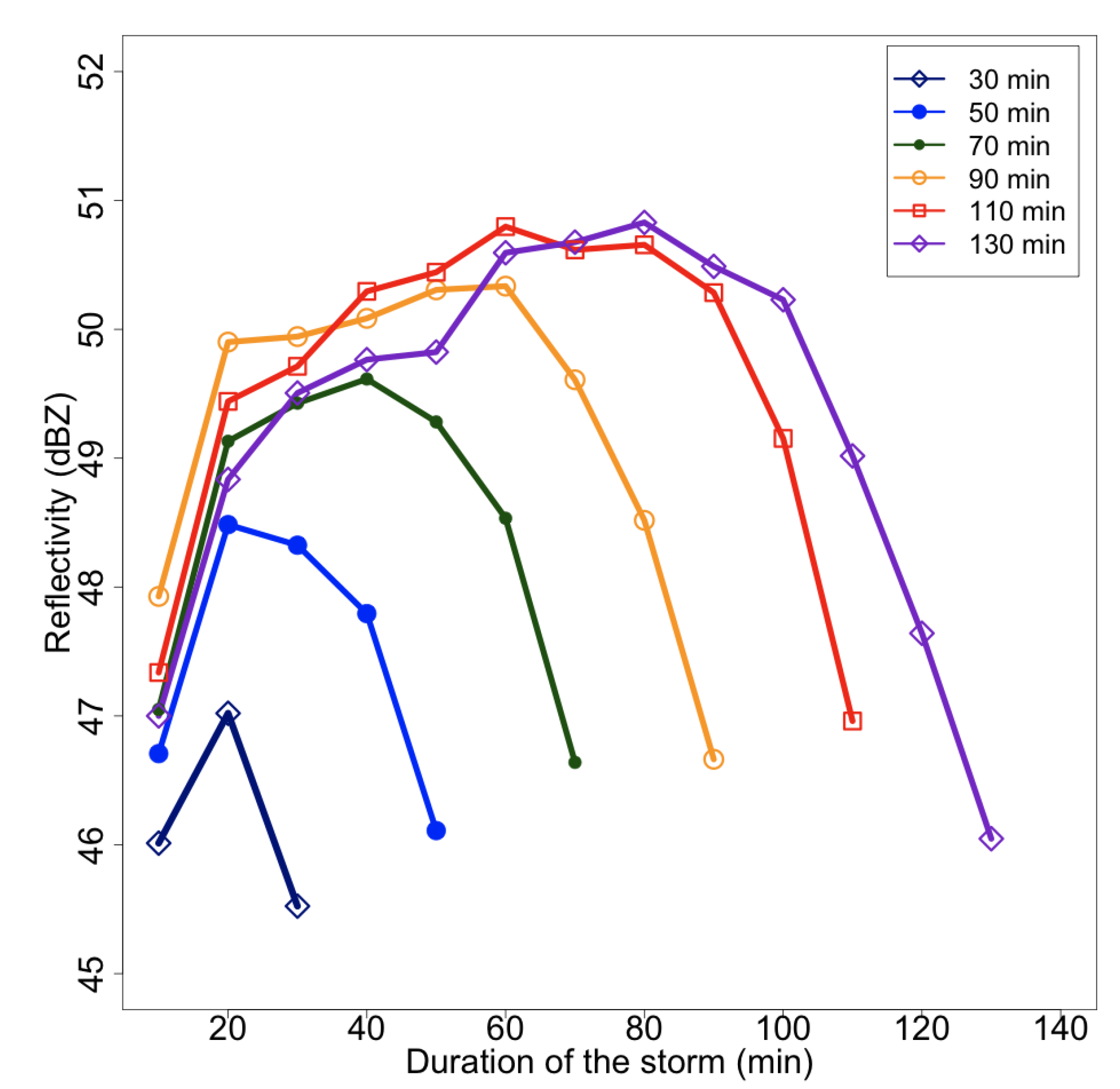
Number of events	18,013	7,757	4,034	2,272	1,405	857	558	364	237	756

), showing a rapid decrease of the tracks with duration. Due to the small number of tracks for the longest durations, a threshold of 100 events was imposed, to make each class statistically significant. In this way, only the cells whose maximum duration is 130 min have been considered in the following analysis. Average values of the maximum reflectivity, evaluated for all tracks belonging to a specific duration class for each instant of their lifecycle, were calculated and they are shown in Figure 3.

According to Figure 3, the cells rapidly increase their reflectivity in the first stages of their lifecycle, generally reaching the maximum value of maximum reflectivity at about the middle of their life or even earlier. After the peak, they slowly dissipate leading to lower values of reflectivity.

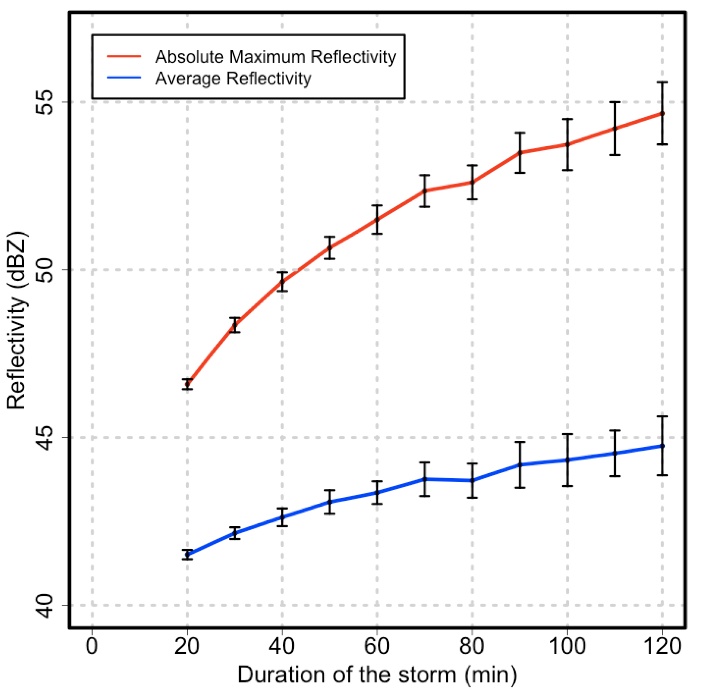
The duration of the tracks is linked with both the absolute maximum and the mean value of reflectivity of the cell during its life cycle, as shown in Figure 4. The average difference between a short and a long life thunderstorm, in terms of maximum reflectivity, is about 6 dB. Therefore a long lasting thunderstorm produces more rainfall than a shorter one for two reasons: (1) the longest persistence; and (2) the highest average intensity.

Despite the fact that it is not possible to forecast the duration of a storm on the only basis of its properties during the first stages of life [18], the results presented in Figure 3 suggest the existence of a relation between the maximum of reflectivity in the first stages of the thunderstorm life cycle and the duration of the entire convective event.

In an unstable atmospheric environment, a convective cell will undergo a rapid development (stronger updrafts are associated with higher instability). At the same time, the availability of unstable moist flows in the low troposphere will increase the chances for the storms to last longer and produce more severe weather.

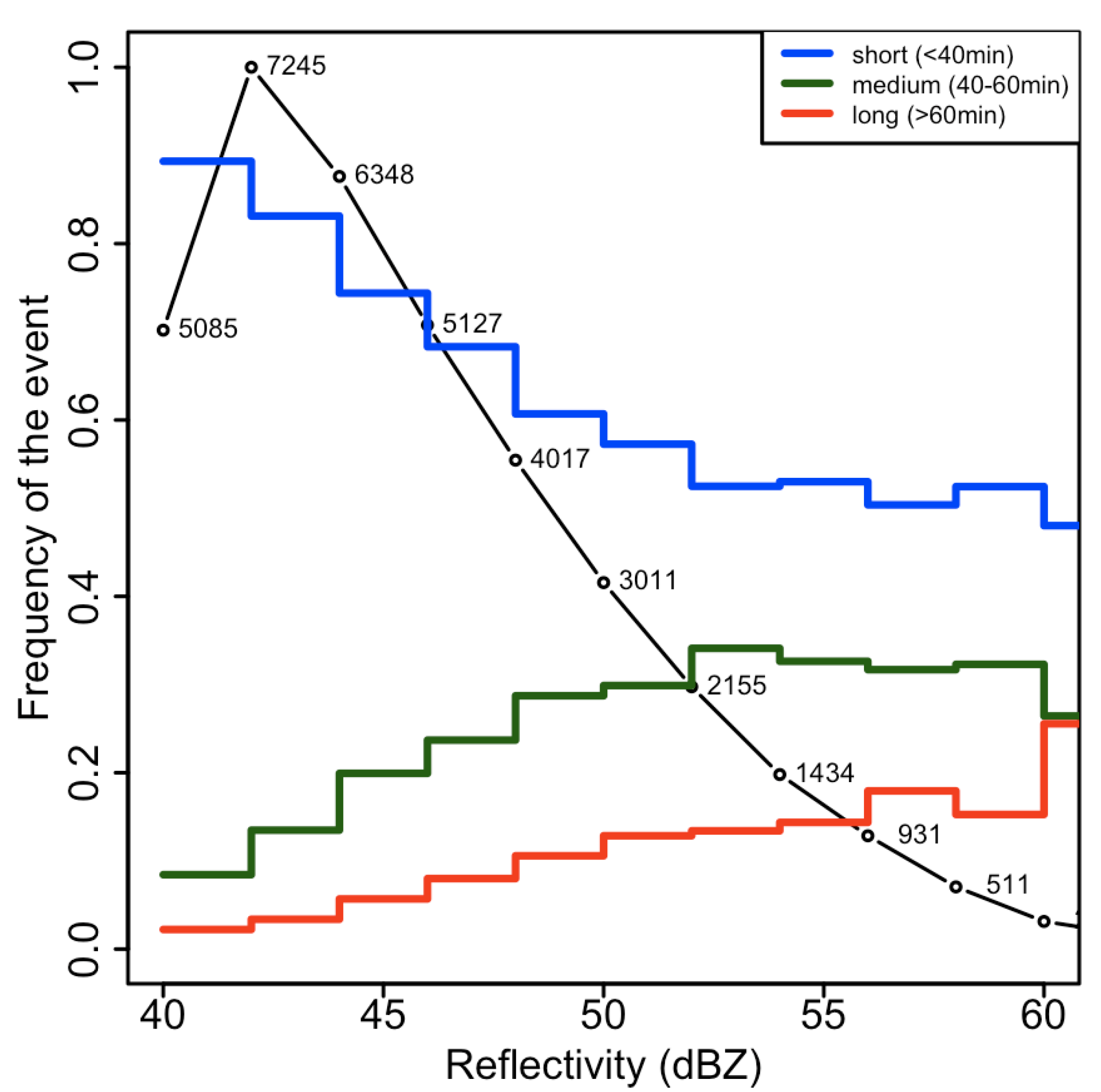
To analyse this behaviour, the tracks were divided into three categories, according to their duration: short (less than 40 min), medium (between 40 and 60 min) and long (more than one hour). The values of maximum reflectivity at the second stage of development of every cell was used in this analysis: they were clustered in 2 dB-wide classes ranging from 40 dBZ to the maximum value recorded.

In this way the relation between the storm duration and the storm maximum reflectivity at the second instant of detection (defined as the second detection of the same cell by the tracking algorithm) was investigated (Figure 5). The percentage of the shortest storms slowly decreases as the maximum reflectivity increases. A storm characterized by a maximum reflectivity in the 40–42 dBZ class at the second instant of detection has a probability of about 90% to deplete in the following 20 min. This probability decreases to about 50% when the maximum reflectivity increases to 55 dBZ. These results may provide a useful statistical clue for an automated nowcasting procedure, especially when the first and second value of the maximum reflectivity for a given cell are low, i.e., there is a very high probability that the considered cell will dissolve shortly.

Figure 5 and Table 2 show how the number of thunderstorms tracked is inversely dependent on duration. In particular, about 49% of the tracks in the dataset survived only 20 min. To focus the attention only on the most relevant phenomena, the shortest tracks (20 min) were excluded from the successive analyses. This choice is strengthened by observing that the rainfall associated with the thunderstorms is rapidly increasing with the duration of the storm (not shown): a storm lasting only 20 min produces about half of the rainfall with respect to one lasting 30 min, and about 16% of a storm lasting one hour. Therefore it is possible to conclude that convective cells lasting less than 30 min have a relatively low impact on the territory.

3.2. The Daily and Seasonal Distribution of Thunderstorms

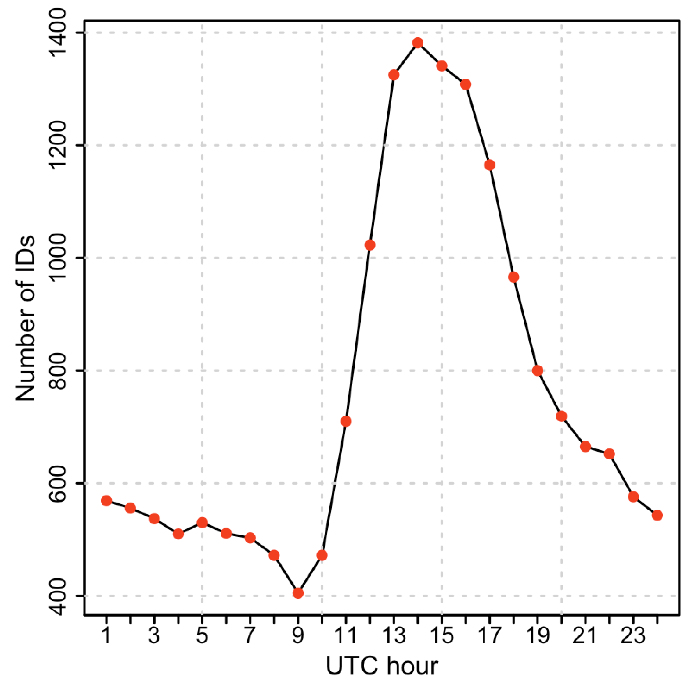
The number of thunderstorms lasting at least 30 min is 18,240 which means about 16 storms per day over the target area. This subset was subdivided according to the hour of the day in which the cell was identified for the first time. To this end, the centroid attributes (position, time, etc.) of the first cell identification are taken as a marker of the tracking itself and are hereafter referred as Initial Detection (ID). This instant is defined as the time in which the maximum reflectivity of the cell exceeds the threshold of 40 dBZ.

The analysis of the hourly distribution of the IDs of each track is plotted in Figure 6, and it shows a rapid and almost linear increase of the number of thunderstorms from the morning (9 UTC, i.e., 11 a.m. local time) to the early afternoon (13 UTC, 3 p.m. local time). After the peak at 2 UTC, the number of events detected decreases continuously and smoothly until 21 UTC (11 p.m. local time) and more irregularly afterwards.

The sharp timing of the peak suggests a prevalence of afternoon ordinary thunderstorms in the target area during the six spring/summer considered months. This is also confirmed by the time delay between the maximum of incoming solar radiation (normally at noon, local time) and the time of the initial detection maximum (3 p.m. local time). This delay is comparable to the theoretical delay between the peak of the forcing solar radiation flux and the peak of the soil surface temperature, in the hypothesis of a sinusoidal thermal forcing [19].

Another foremost feature is the delay found in the morning, between the sunrise and the moment of the abrupt increase of the initial detection IDs (around 11 a.m. local time). The reason is likely related to the feeble solar radiation in the first hours of the morning, which prevents the thermals from overcoming the resistance of the boundary layer inversion. Later in the morning, once the thermals become able to reach the lifting condensation level (LCL), over which the atmosphere often becomes unstable, a quick growth in the number of thunderstorms is observed (threefold increase over three hours).

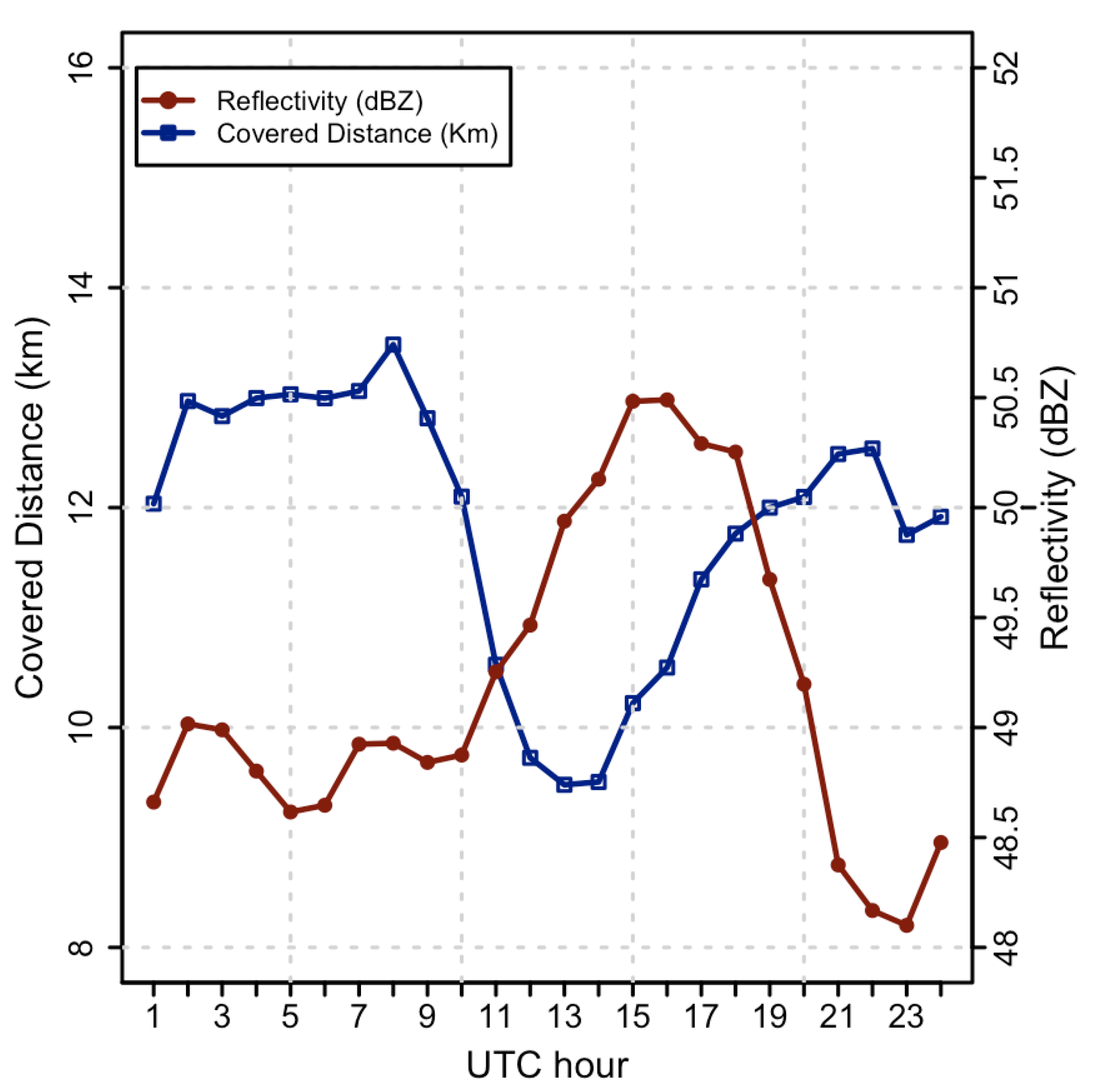
Figure 7 shows other data which may help to understand the dynamic of the thunderstorm daily variability: the maximum reflectivity and the distance travelled by the cells. To obtain the latter parameter (which represents the mean values of the distance travelled by a thunderstorm during its life cycle) the distance between the first and the last detection was calculated. With this method, however, no information about the irregularity of the trajectory is retained. The daily variation of both parameters is small (2 dB for reflectivity, and 5 km for the distance), but still significant. The maximum reflectivity shows a peak in the late afternoon (with an irregular plateau of 50.5 dBZ between 14 UTC and 17 UTC, i.e., 16 and 19 local time), occurring about 2–4 h after the observed the first detection maximum (Figure 6). A completely opposite behaviour is shown by the travelled distance (Figure 7), which is quite noisy at night and characterized by a well defined minimum during the afternoon (when thunderstorms are more frequent and intense). These results confirm the previously argued hypothesis about the prevalence of ordinary storms during the hottest hours of the day. In fact, these thunderstorms are often quasi-stationary and their downdrafts usually self-destroy their updrafts in the active phase of the storm [20].

As the data cover a period of 6 months, it was also possible to analyze the monthly variability of the above-mentioned physical parameters (not shown). The strongest thunderstorms are detected in July, the weakest in April. The mean maximum reflectivity difference between these two extremes is almost 4 dB. The distance travelled by thunderstorms is low from April to July, then peaks in August, and again it slightly decreases in September. The largest values observed in August and September may be explained considering that: (1) the higher number of cold advections, typical of the late Summer in this area, often generates storms along the cold front, thus able to cover longer distances; (2) the high values of the sea surface temperature in the late Summer favour the storms generation over the sea, which, as discussed later in Section 3.6, often travel longer distances.

3.3. The Spatial Distribution of IDs Over the Region

The analysis presented in the previous section highlighted the general behavior of convective cells over the entire target area. The objective of the following analysis is to focus on the small scale features, in order to detect possible preferential regions for thunderstorm development. The whole target area was split into pixels of fixed dimension, and all thunderstorms whose ID lay in the same pixel were studied together. In such way, different statistics regarding all the parameters studied were extracted.

In order to obtain a good spatial resolution and a low level of noise, an oversampling technique was used in order to extract a clearer pattern from a high-resolution map. In the specific case, the starting map has a resolution of 2 × 2 km². The oversampling was carried out adopting the Barnes 2D distance-dependent weight function [21] calculating the weighted average of each pixel with all the neighboring pixels in a radius of 5 km, according to the equation:

(3)

where t_k ^smoothed and t_i ^original represent respectively the pixels after and before the smoothing, r_i,k is the distance between the i-th and k-th pixels. The length scale L has been set to two times the data spacing (L = 4 km), according to [22].

Figure 8 shows the spatial distribution of the IDs density after the application of the oversampling algorithm. The highest densities are located on the western side of the target area, and four relative maxima are evident, from North to South: (1) near Biella (at the southeastern border of the Valle d’Aosta); (2) the Canavese region (from Val di Susa to Valli di Lanzo); (3) East of Mount Monviso; and (4) near Genova, over Mount Beigua, on the Apennines. The highest IDs densities are located close to the mountains, while there is a steep density decrease over the valleys and plains. There are other three areas where the densities are lower than the aforementioned maxima, but still relevant: (1) a large area near Torino; (2) an oblongly linear pattern along the Susa valley, at West; and (3) a scattered group of relative maxima near the Lake Maggiore, at the border with Lombardy region, at the North-East. On the other hand, Ligurian Sea and the provinces of Asti and Alessandria, placed on the eastern side of Piemonte region, show lower storm densities.

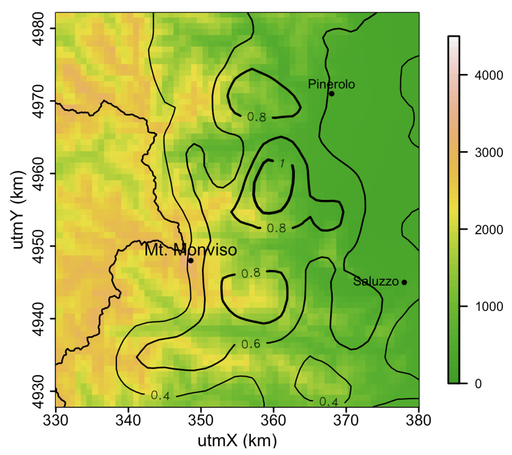
The two relevant maxima near the Mount Monviso and West of Torino are hereafter analyzed in more detail. A zoom over the Monviso area clearly shows two distinct IDs density maxima located at the eastern foot of the mountain (Figure 9). This mountain, whose top exceeds by about 1000 m the neighboring orography, forces the humid westward-moving air blowing from the plains to lift, increasing the chance of storm generation when the atmosphere is conditionally unstable. The isolines of IDs density seem to embrace the mountain tops in this area. The two symmetric relative maxima, disposed along the two sides of the high Po Valley, represent an outstanding example of storms triggered by the topography.

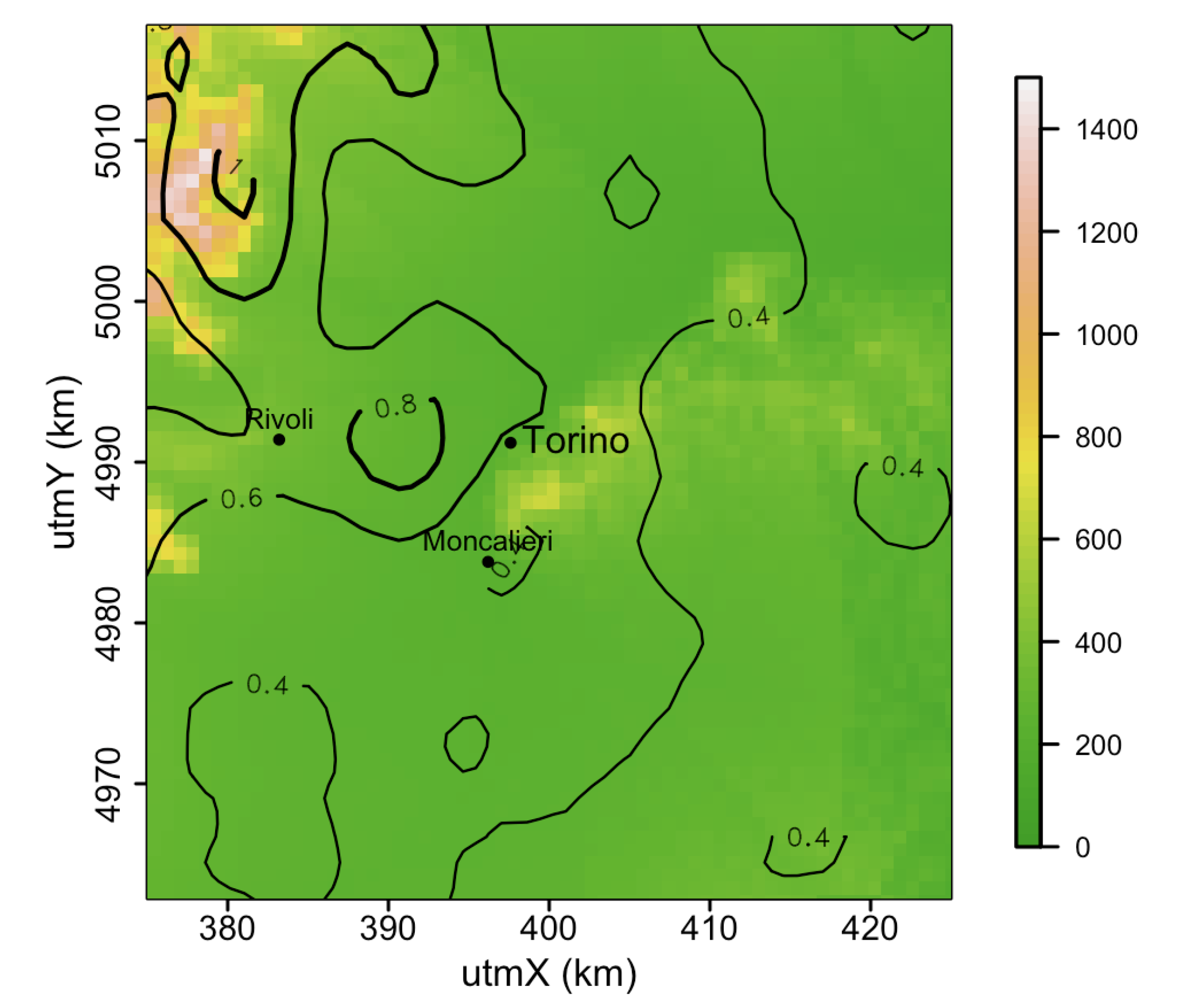
The value of IDs density relative maximum in the Torino area (Figure 10) is about the 30% less with respect to those near Mount Monviso. However, this area deserves a special interest due to the large number of inhabitants (about 1 million) and infrastructures. The maximum is located over the western side of the city, near the entrance of the Val di Susa which is the most highly populated part of the city.

To further investigate this maximum of IDs density, the main properties of the storms over the Torino area (defined as a box of 40 × 40 km centred over the city) was examined: whilst duration and mean covered distance are generally equal to the averages values of the target area, some differences are found in the reflectivity values. Storm occurring over the Torino area show higher values of both maximum reflectivity and mean value of reflectivity. In terms of precipitation, they discharge about 20% more rainfall than the average of storms over the target area.

To deepen this peculiar feature, a map of the distribution of average maximum reflectivity was computed (not shown). The increased reflectivity maximum is particularly evident about 20–40 km on the eastern side of the city. There are many possible causes of such a maximum, as the local breeze circulation associated to the peculiar topography of the area, or the close distance between the area and the Bric della Croce radar, or even possibly a Urban Heat Island effect. In any case, the analysis of this feature goes beyond the scope of this study.

3.4. The Spatial Distribution of IDs in the Different Hours of the Day

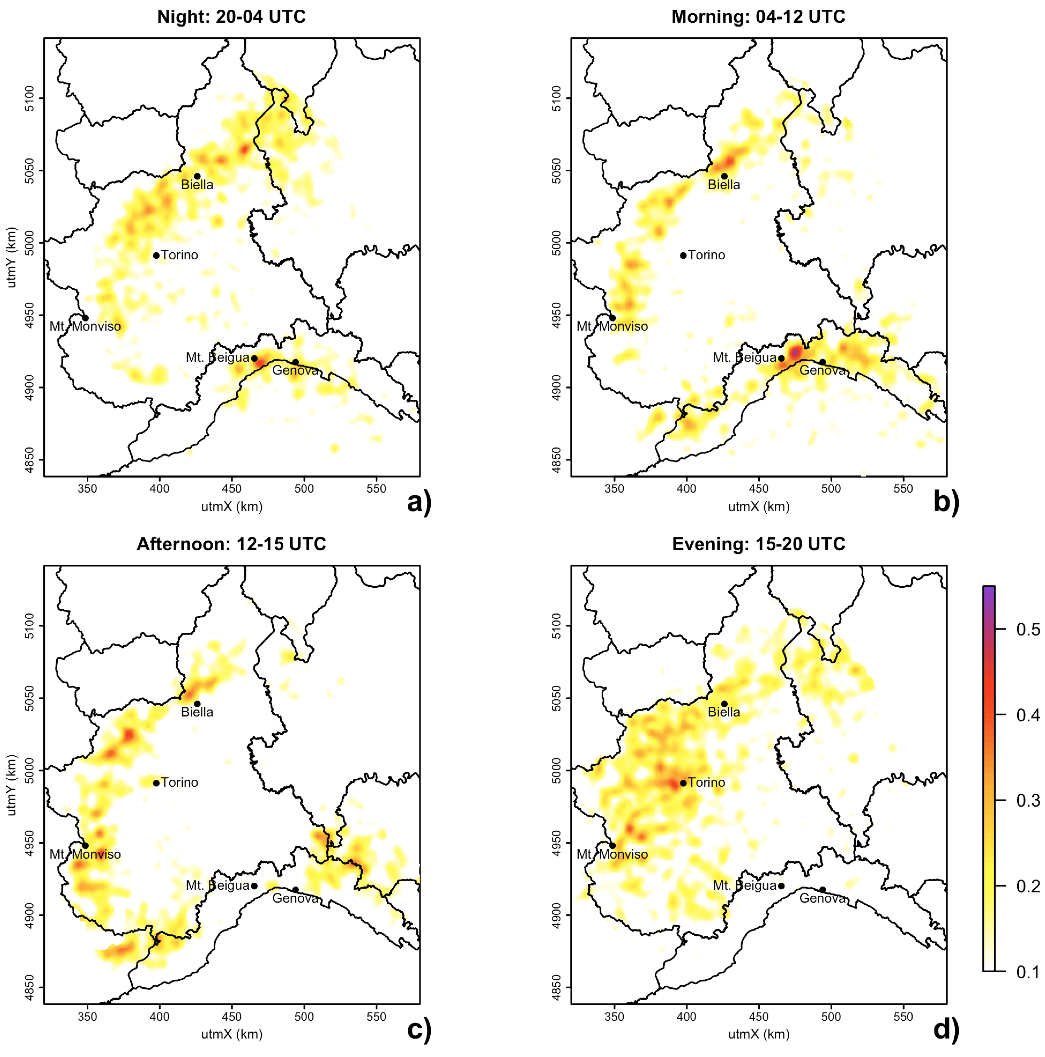
Figure 6 has shown that the largest number of IDs is concentrated in the afternoon hours. The variation of the location of the IDs during the day is hereafter considered. To this end, the day is subdivided in four periods: night (20–04 UTC), morning (04–12 UTC), afternoon (12–15 UTC) and evening (15–20 UTC).

During the morning (Figure 11b) many maxima are located in a narrow line skirting the Alps (in the so-called prealpine area). During the night (Figure 11a), in addition to the several density peaks located in the area close to the mountains, some other maxima are visible over the plains, so that storm locations at night look definitely more scattered than in the morning.

This specific pattern can be attributed to the prevailing mechanisms of thunderstorm generation during daytime and nighttime. In the morning the storms are mainly triggered by the heating brought by the solar radiation. At night time, due to radiative cooling of the valleys slopes, the storms may often be generated by the mountain-valley breeze, triggering convection where the mountain cool downward-flow encounters the warmer air over the plains.

Another peculiar point is that, during night-time, few IDs are observed over Liguria, except a maximum close to Mount Beigua, near Genova. On the contrary, in the morning hours, Liguria shows a high number of maxima, favored by the interaction of the daytime sea breeze circulation (directed towards the land) with the mountains.

Figure 11c,d shows the observed pattern of IDs distribution during the afternoon and the evening hours. In the afternoon (Figure 11c), thunderstorms are generated over almost the whole Alpine Arc. This pattern partially overlaps the morning density distribution, the main difference being represented by the storms detected on the French side in the South-Western sector. This feature clearly strengthen the hypothesis of the prevailing radiative origin of the storms in the mountainous regions: the exposure of the mountain sides to the solar radiation reinforces the breeze which favor the onset of enhanced upward motions. Indeed, most of the mountain slopes oriented Southward or South-eastward (i.e., those located in the western and northern sectors) show their local maxima of IDs already in the morning, while the South-westward oriented slopes in France show a relevant storm density in the afternoon.

The distribution of the evening maxima (Figure 11d) looks less defined and highly scattered. There are many maxima distributed not only along the Alps and Prealps, but also over the plains, covering the entire Western Piemonte. A wide area of maxima covers the area between Biella (at North) and the Canavese, at North-West. The Torino area shows a large density of IDs too, confirming the local common experience that in Torino thunderstorms frequently occur in the late afternoon.

Summarizing the above-mentioned findings, it can be stated that the most favorable areas for triggering storms are strongly linked in North-western Italy to the effect caused by the orographic reliefs and in particular to the presence of mountain-induced breeze regimes. This is particularly evident in some areas, specifically near to Mount Monviso and Mount Beigua, where maxima highly localized both in space and time are present.

3.5. The Preferential Direction of the Storms

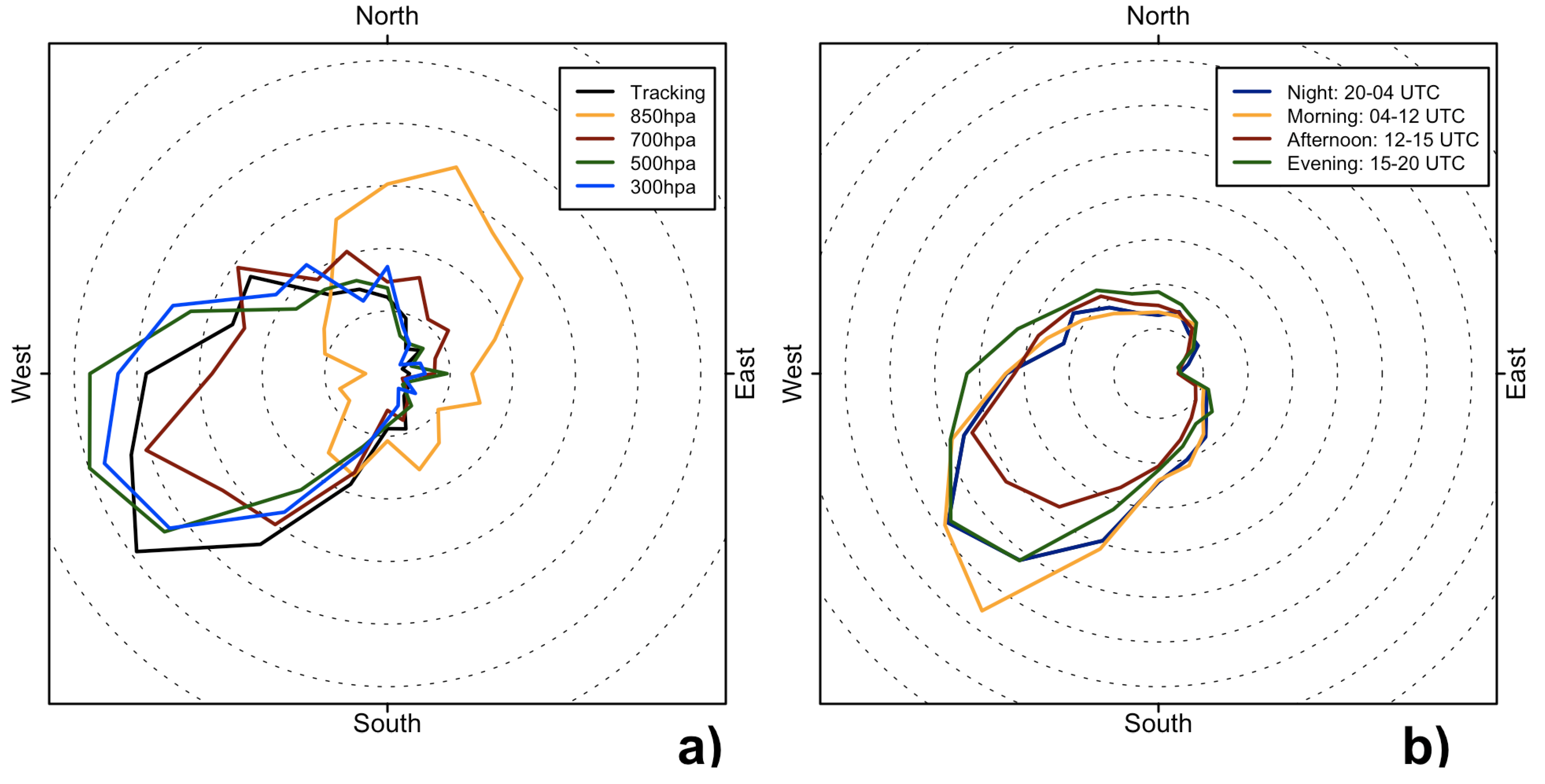
This section focuses on the tracked storms’ motion. To this end, using the starting and final point of each tracking, angles representing the average direction of the storm were evaluated. The obtained angles were grouped in sectors 10 degrees wide, and are represented as provenance directions, in order to be comparable with those of the upper-air winds (see Section 3.6). Figure 12a (black line) shows the distribution of the daily average of the above-mentioned angles. A prevailing direction emerges from this figure: the majority of the events moves from the sectors located between SSW and W, with a peak around South-West. About the 26% of the storms moved from sectors between 200°and 240°. In addition to this, in Figure 12b we reported the distribution of the tracking in different moments of the day, as defined in Section 3.4. Interestingly, even if the areas of storm triggering change significantly during the day, the average distribution of the storms direction is almost the same. This finding will be analyzed more in detail in Section 3.6.

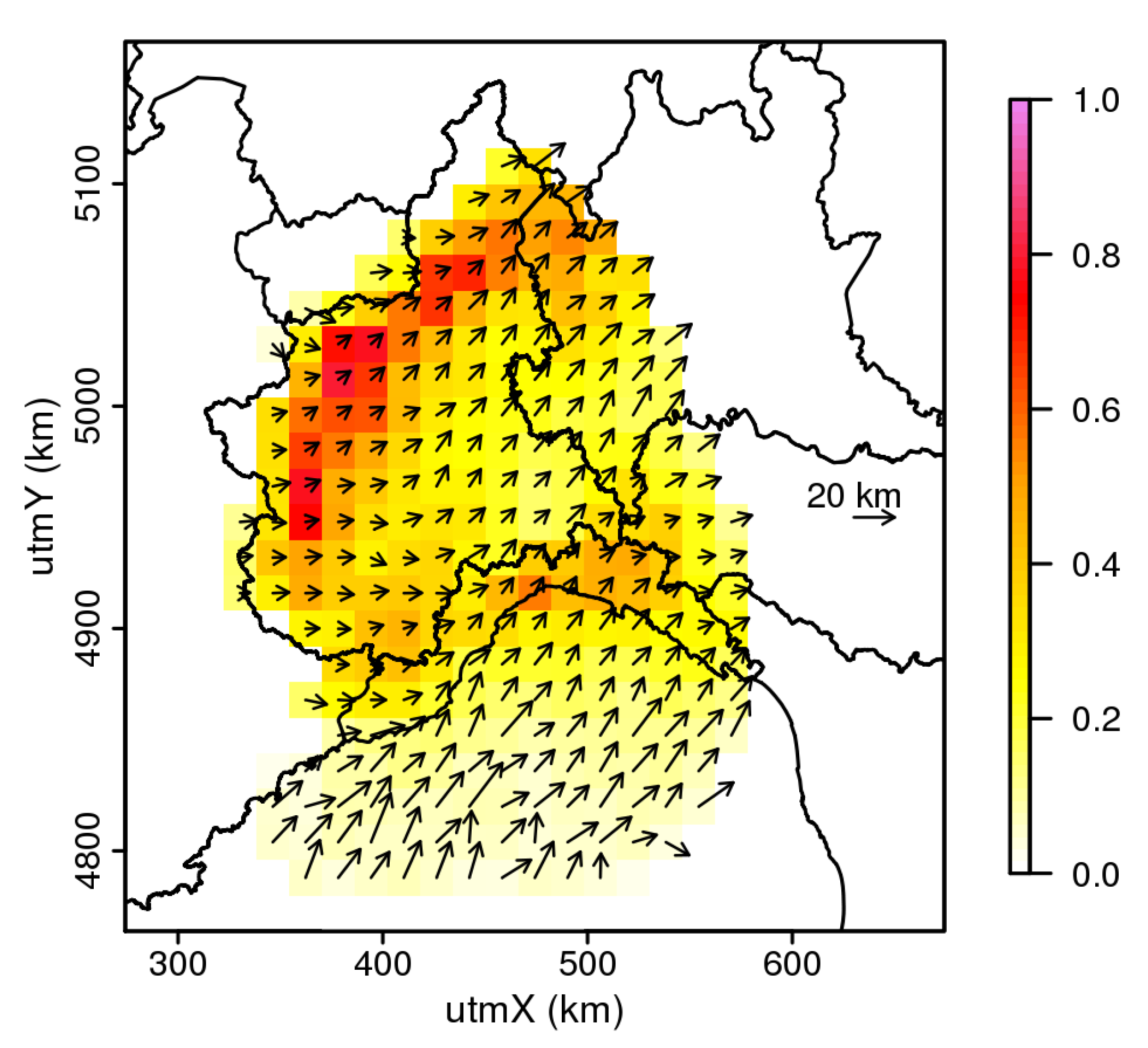
In any case, in order to get more insight on the spatial distribution of these angles, the domain was subdivided in a 16-km resolution grid box. The mean values of the direction and distance travelled, as well as the IDs mean densities, were calculated. To favour the reader, instead of the direction of provenance, the thunderstorms heading is reported in Figure 13. To keep the statistic results significant, the values of direction and travelled distance were plotted only when a sufficient number of storms (more than 5 events) was found in each pixel.

The figure highlights different preferential storm heading in the Northern (heading North-West) and South-Western (heading West) Piemonte. The field is relatively smooth and shows a gradual clockwise rotation and increased travelled distance in the central Piemonte, moving from the mountains to the plains. Concerning the Liguria region, the sparse storms which originate over the Ligurian Sea move from South-West to North-East and cover longer distances respect to the in-land storms.

3.6. The Relation with Free Atmosphere Winds

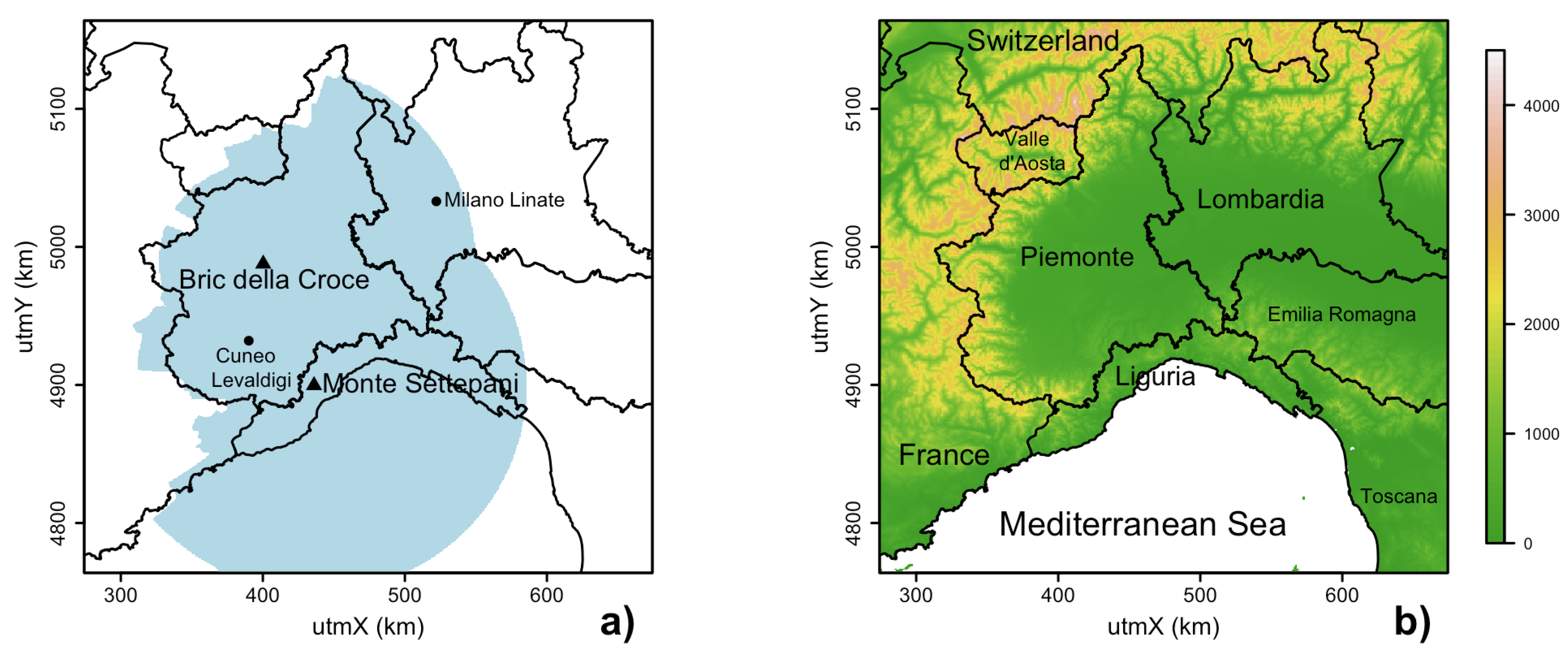
The results of the previous section suggest the existence of a possible correlation between the direction of the storms and the wind. Therefore the identification of an atmospheric level whose wind mostly affects the direction of the storms was carried out. To this end, all radiosoundings performed at 00 UTC and 12 UTC at the station of Cuneo Levaldigi (located in the Southern Piemonte) were analyzed. When these data were not available, those from the station of Milano Linate were used instead. Both stations are located in the target area, as shown in Figure 1.

In order to maintain a daily basis for the analysis (since the number of storm per day is small) we computed for each day the average of the three soundings (00, 12, 24 UTC), with different weights (0.25, 0.50, 0.25). In order to consider the resulting average, at least two over three soundings must be retrieved (otherwise the day is considered missing). The total number of days in the analyzed period is 1098, and for 1087 days it was possible to define a daily value from radiosounding. We remark that the triple mean on the sounding data is performed to have a value representative for the whole day. In a real-time application the most recent sounding should be used or alternatively a sounding from a numerical model for a given lead time forecast.

Convective events occurred in 682 days, and for 675 days the radiosounding were available (i.e., about the 99% of the days). Four levels were selected for this analysis: 850, 700, 500 and 300 hPa. The first one may be considered as representative of the boundary layer, the second of the lower free troposphere (within the Alps), the third one of the free atmosphere (above the Alps), and the latter of the high troposphere, immediately below the tropopause. The direction of provenance was considered for the storm tracks, in order to make the comparison with the wind direction measurements.

The distribution of the four level wind directions from radiosoundings and the storm track directions are reported in Figure 12. It is evident that only the winds in the three upper layers have a distribution similar to that of the storm tracks. Moreover, as shown in Figure 12b, the distribution of the storm is almost independent from the different hours of the day, suggesting that the main role in heading the storms over the target area can be addressed to the mid-tropospheric wind and that local breeze system can probably only affect the triggering areas. In any case, the selection of the most representative wind level for the storm motion is an issue still debated in literature. There have been several different proposals, likely related to the local climatology of the studied area. For instance, in the US, usually the mean wind in the lower layers of the troposphere has been considered (Johns et al. [23] used the mean wind in the first 6 km of troposphere). In Europe other authors [24] have used the mean wind between 2 and 5 km of altitude.

To get more quantitative results the correlations among winds at different levels and storm tracks (direction, speed module, speed vectors) were investigated. For the storm track directions and speed vectors, correlation coefficients (ρ²) were evaluated. Since these data are angles or vectors, they were calculated using their components, adopting the vector correlation introduced by Crosby et al. [25]. When data considered are angles (i.e., in case of track directions), the vector length is supposed unitary. Values of ρ² calculated in this way range between 0 (absence of any correlation) and 2 (perfect correlation). For the speed module, instead, the correlation coefficient was calculated as usual, adopting the Pearson method. Considering the different choices made by different authors and the fact that a similar analysis has not been carried out previously on the Italian territory, also the mean values in the tropospheric layers 850–500 hPa and 700–500 hPa were included in the analysis. The results are reported in

Table 3. Values of the correlation coefficient for the daily mean values. Vector correlation introduced by Crosby et al. [25] for storm directions and speed vector is used. Pearson correlation for storm speed module is instead adopted.

	Wind - Storm directions	Wind - Storm speed module	Wind - Storm speed vector
	ρ2(0–2)	ρ(0–1)	ρ2(0–2)
850 hPa	0.14	0.14	0.25
700 hPa	0.89	0.56	0.95
500 hPa	1.03	0.59	1.03
300 hPa	0.70	0.39	0.75
850→500 hPa	1.05	0.46	1.09
700→500 hPa	1.07	0.50	1.11

.

The highest correlation is observed considering the mean value of wind in the layer 500–700 hPa, i.e., between about 3000 and 5500 m a.s.l.. Very high values for correlation coefficients have been also obtained considering the 500 hPa level, suggesting that the adoption of the wind field at this unique level could be very useful for the operational nowcasting. The values of the correlation coefficient also confirm that storm paths are not correlated with 850 hPa winds (i.e., about 1500 m). This fact is not surprising as, in the target area, the altitude of many Alpine mountains is higher than this level, thus the circulation during summertime is mainly affected by the complex topography and by the correlated system of local winds. For this reason, in the analyzed area the approach of Johns et al. [23] is not convenient.

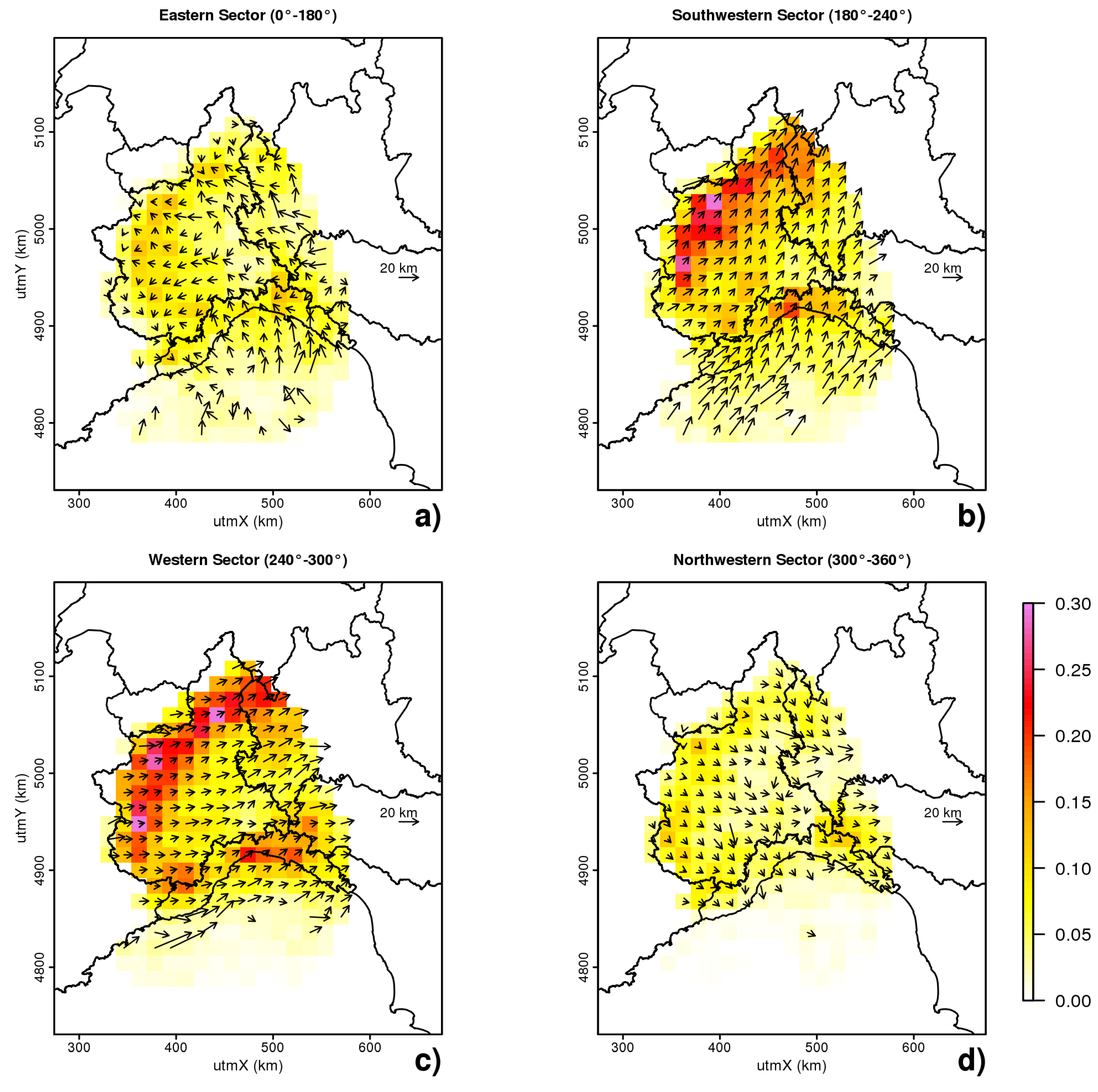
In order to discriminate between different synoptic conditions, a further analysis was carried out considering the direction of the mean wind speed in the layer 500–700 hPa. Since the wind direction in the mid-troposphere is not uniformly distributed, all storm tracks were subdivided into four sectors with different angular extent: East (directions of provenance between 0° and 180°, with a total of 3636 tracks); South-South-West, 180°–240°, with 5734 tracks; West, 240°–300°, with 5930 tracks; and North-North-West, 300°–360°, with 2230 tracks. The results are plotted in Figure 14 and the statistical summary is reported in

Table 4. Statistics on the occurrence of storms and upper air winds (based on radiosounding mean wind between 700 and 500 hPa).

	East	SSW	West	NNW
Number of days	243	190	400	254
Number of stormy days (at least one storm)	143	156	259	117
Incidence of stormy days	59%	82%	65%	46%
Number of storms tracked	3636	5734	5930	2236
Number of storms per stormy day	26.22	36.75	22.89	19.11
Mean Wind Speed (m s−1)	7.35	11.50	10.96	8.97

. This subdivision was carried out adopting the 12 UTC radiosounding for storms occurring between 06 UTC and 18 UTC, and the radiosounding at 00 UTC for the remaining storms.

The majority of thunderstorms and the highest probability of occurrence of a thunderstorm are both associated with Westerly or South-Westerly wind, as shown in Table 4. This behaviour is likely due to the different amount of moisture associated with the dominant mid-tropospheric flow. In North-Western Italy, the North-Westerly flows are normally drier than those coming from the other sectors, due to the katabatic winds (foehn wind) originated across the Alpine mountain reliefs [26]. On the contrary, despite the air coming from Eastern sectors is originally dry, during the travel over the Po valley its moisture content increases due to the relatively high humidity over the plains. Finally, the South-Westerly flows carry humidity from the Mediterranean Sea, and the Westerly flows from the Atlantic Ocean, thus increasing the possibility of convective precipitations (82% and 65%, respectively, of stormy days from these sectors).

Figure 14 clearly shows the high impact of the mean wind direction in the layer 500–700 hPa on the direction of the storm tracks. The lengths of the vectors in the figure also reveals that the distance travelled by the storms varies accordingly to the mean wind speed. Mean wind intensities are different in each sector analyzed: as shown in Table 4, the mean wind speeds are generally lower for the Eastern and North-North-Western sectors, and higher for the South-South-Western and Western sectors. Storm track travelled distances show a similar behaviour.

Despite the differences regarding the number of events and the distance covered by the storms, it is worth noting that the spatial distribution of the IDs densities show little variability at the 16 km resolution, for different upper air winds (Figure 14). Therefore, whilst the midtropospheric wind shows a considerable impact on the movement of the storm, it does not influence significantly the location of the areas most suitable for generating thunderstorms, generally located along the Alpine foothills arc.

4. Conclusions

In this paper, a comprehensive study of convective storms over North-Western Italy have been performed in order to establish a starting point in the climatological analysis of those events, given the scarcity of similar previous studies carried out over the Alps and the complete lack regarding Italy.

To this end, all thunderstorms occurred during the warmest months (April to September) of a 6-year period (2005–2010) over the North-Western Italy were analyzed considering the data collected by the Arpa Piemonte weather radar network. The tracks of each storm were evaluated using a storm-tracking algorithm (based on the COTREC method) operationally used at Arpa Piemonte. A preliminary pre-processing operation, aimed at excluding from the database all tracks referring to storms too weak or located in areas affected by poor radar visibility, was performed. Afterwards, several characteristics of the storms were analyzed: the duration of the storms, the spatial and the temporal distribution of the tracks, their direction and the travelled distance.

The results of the global analysis of the storm tracks distribution allowed to quantify experimentally some features of thunderstorms qualitatively already known: the seasonal distribution of the storms and the daytime distribution were analyzed, showing that storms are more frequent and intense in July and August and during the afternoon hours. Moreover, the timing of the maximum occurrence and intensity are well correlated with the periods of the year and day in which the soil temperature is higher, suggesting the prevalence in this region of afternoon ordinary storms.

A deeper analysis on the storm development revealed a typical life cycle. The maxima of precipitation, intimately connected with the maximum reflectivity, are often recorded in the first half of the storm life, while the maxima of the areal extension of storms are found in the last part of the life cycle. Interestingly, long lasting storms usually reach higher values of reflectivity, suggesting that the impact (in terms of rainfall) of storms with high duration is notably greater than short lasting ones.

Another foremost characteristic, potentially useful for the nowcasting of the storm evolution, emerged: a meaningful correlation between the intensity of the storms in the first stages of their life cycle and the duration of the storms is found. In particular, a convective cell showing relatively low values of reflectivity during the first stages will have a very high probability of dissolving quickly: for example, a cell showing a maximum reflectivity not exceeding 45 dBZ in the first 20 min of its life will decay in the following 10 min with a probability of about 90%.

The analysis of the spatial distribution of the thunderstorms allowed to highlight some specific areas most suitable for the generation of convective cells. These regions are located in proximity of hills or mountains, suggesting an active role of the topography in triggering storms. Moreover, the variation of the distribution of the above mentioned areas during the different hours of the day suggests that the solar radiation plays a dominant role in the generation of convective cells. The analysis also showed that the distance travelled by the storms is shorter in proximity of the mountains and larger over the plains and sea. Therefore, it is possible to infer that the storms triggering over the considered region is mainly caused by the combination of solar radiation and orographic reliefs, which favors the development of local scale breeze system.

The last part of the study was devoted to analyze the correlation among the storm direction, the travelled distance and the mean wind speed. Measurements of wind speeds were obtained from the radiosounding station of Cuneo Levaldigi and Milano Linate. The results show that preferential direction of movement of the storms is strictly linked with the mean wind in the layers between 500 hPa and 700 hPa, i.e., well above the boundary layer and also above the mean level of the Alpine mountains. A last analysis was carried out in order to characterize the storms with respect to the synoptic condition: the South-Westerly mean wind emerged as a key element to favor the triggering of the convective activity over the target area. On the other side, it is worth noting that the mean wind has a negligible impact on the spatial distribution of the storms.

Finally, it is remarked that the whole dataset described in this work, which could be easily extended in the future, gives the opportunity to create an operational archive that may provide important information able to improve the nowcasting activities of the ARPA Piemonte weather service. A larger dataset will also provide the opportunity to explore some of the findings that, due to the short temporal extension of the present dataset, have been not analysed in this work. In this way, we hope to infer some more details about the maximum of reflectivity above the Torino area, investigating its possible relation with the Urban Heat Island effect. A dataset encompassing a larger number of years will also give the opportunity to study possible climatic effects, as the ones associated with the North Atlantic Oscillation, on the thunderstorm distribution over the North-Western Italy.

References and Notes

1. Kelly, D.L.; Schaefer, J.T.; Doswell, C.A., III. Climatology of non-tornadic severe thunderstorm events in the United States. Mon. Weather Rev. 1985, 113, 1997–2014. [Google Scholar] [CrossRef]
2. Hocker, J.E.; Basara, J.B. A Twelve-Year Climatological Analysis of Severe Local Storms Observed by the Oklahoma Mesonet. In Proceedings of the Symposium of the Challenges of Severe Convective Storms, Atlanta, GA, USA, 29 January-3 February 2006; p. 1.21. [Google Scholar]
3. Changnon, S.A. Climatography of thunder events in the conterminous United States. Part I: Temporal aspects. J. Clim. 1998a, 1, 389–398. [Google Scholar] [CrossRef]
4. Changnon, S.A. Climatography of thunder events in the conterminous United States. Part II: Spatial aspect. J. Clim. 1998b, 1, 399–405. [Google Scholar] [CrossRef]
5. Falconer, P.D. A radar-based climatology of thunderstorms days across New York State. J. Clim. Appl. Meteorol. 1984, 23, 1115–1120. [Google Scholar] [CrossRef]
6. Outlaw, D.E.; Murphy, M.P. A Radar-Based Climatology of July Convective Initiation in Georgia and Surrounding Area; NOAA Eastern Region Technical Attachment 2000/04; National Oceanic and Atmospheric Admistration, US Department of Commerce: Washington, DC, USA, 2000; p. 15. [Google Scholar]
7. Jaeneke, M. Radar Based Climatological Studies of the Influence of Orography of Thunderstorms Activity in Central Europe. In Proceedings of the 30th International Conference on Radar Meteorology, Session 12A, Munich, Germany, 19–24 July 2001; p. 12A.5. [Google Scholar]
8. Horvath, A.; Acs, F.; Seres, A.T. Thunderstorm climatology analyses in Hungary using radar observations. Idojaras 2008, 112, 1–13. [Google Scholar]
9. Rudolph, J.; Friedrich, K.; Germann, U. Relationship between radar-estimated precipitation and synoptic weather patterns in the european alps. J. Appl. Meteorol. Climatol. 2011, 50, 944–957. [Google Scholar] [CrossRef]
10. ARPA Piemonte is a regional organization for environmental protection. In Piemonte, this agency is in charge of the meteorological, hydrological and geological service, as well as the responsibilities for the the local civil protection. The ARPA Piemonte meteorological network is composed by more than 400 meteo-hydrological stations, two radiosounding stations and two operational weather radars.
11. Bringi, V.; Chandrasekar, V. Polarimetric Doppler Weather Radar: Principles and Applications; Cambridge University Press: Cambridge, UK, 2001; p. 636. [Google Scholar]
12. Liu, H.; Chandrasekar, V. Classification of hydrometeors based on polarimetric radar measurements: Development of fuzzy logic and neuro-fuzzy systems, and in situ verification. J. Atmos. Ocean. Technol. 2000, 17, 140–164. [Google Scholar] [CrossRef]
13. Gourley, P.; Tabary, P.; Parent, J. Classification of Hydrometeors and Non-Hydrometeors Using Polarimetric C-Band Radar. In Proceedings of the 32nd Conference on Radar Meteorology, Albuquerque, NM, USA, 10 June 2005; p. 11R.4. [Google Scholar]
14. Handwerker, J. Cell tracking with TRACE3D: A new algorithm. Atmos. Res. 2002, 61, 15–34. [Google Scholar] [CrossRef]
15. Doviak, R.J.; Zrnic, D.S. Doppler Radar and Weather Observations; Academic Press: Waltham, MA, USA, 1984. [Google Scholar]
16. Rinehart, R.E.; Garvey, E.T. Three-dimensional storm motion detection by conventional meteorological radar. Nature 1978, 273, 287–189. [Google Scholar] [CrossRef]
17. Mecklenburg, S.; Schmid, W.; Joss, J. COTREC–A Simple and Reliable Method for Nowcasting Complex Radar Pattern Over Complex Orography. In Proceedings of the Final Seminar of COST-75: An Advanced Weather Radar Systems, Locarno, Switzerland, 23–27 March 1998; Volume 61, pp. 441–450. [Google Scholar]
18. MacKeen, P.L.; Brooks, H.E.; Elmore, K.L. Radar reflectivity–Derived thunderstorm parameters applied to storm longevity forecasting. Weather Forecast. 1998, 14, 289–295. [Google Scholar] [CrossRef]
19. Stull, R. An Introduction to Boundary Layer Meteorology; Kluwer Academic Publishers: Dordrecht, The Netherlands, 1989; p. 666. [Google Scholar]
20. Buzzi, A.; Fantini, M.; Lippolis, G. Quasi-stationary organized convection in the presence of an inversion near the surface: Experiments with a 2-D numerical model. Meteorol. Atmos. Phys. 1991, 45, 75–86. [Google Scholar] [CrossRef]
21. Barnes, S.L. A technique for maximizing details in numerical weather map analysis. J. Appl. Meteorol. 1964, 3, 396–409. [Google Scholar] [CrossRef]
22. Koch, S.E.; DesJardins, M.; Kocin, P. An interactive barnes objective map analysis scheme for use with satellite and conventional data. J. Clim. Appl. Meteorol. 1983, 22, 1487–1503. [Google Scholar] [CrossRef]
23. Johns, R.; Doswell, C.A., III. Severe local storms forecasting. Weather Forecast. 1992, 7, 588–612. [Google Scholar] [CrossRef]
24. Kyznarova, H.; Novak, P. Development of Cell-Tracking Algorithm in the Czech Meteorological Institute. In Proceedings of WSN05—World Weather Research Programme—A Symposium on Nowcasting and Very Short Range Forecasting, Toulouse, France, 5-9 September 2005; p. 6. [Google Scholar]
25. Crosby, D.S.; Breaker, L.C.; Gemmill, W.H. A proposed definition for vector correlation in geophysics: Theory and application. J. Atmos. Oceanic Technol. 1993, 10, 355–367. [Google Scholar] [CrossRef]
26. Fratianni, S.; Cassardo, C.; Cremonini, R. Climatic characterization of foehn episodes in Piedmont, Italy. Geogr. Fisica Din. Quat. 2009, 32, 15–22. [Google Scholar]
Figure 1. (a) The area considered during the analysis: triangles and dots show respectively the location of weather radars and of radiosounding stations; (b) The altimetry of the region.
Atmosphere 03 00033 g001
Figure 2. Maximum reflectivity map (projection to the ground of the maximum reflectivity along the vertical) from the Bric della Croce radar on 13 August 2010 at 20:20 UTC before (a) and after (b) the clutter removal procedure. The map is shown on a reduced 75 km range domain for clarity, with range rings overplotted every 25 km. The Alps (on the West and North side) and Apennines (South) are clearly visible in the original data (left panel), with peak reflectivities above 60 dBZ.
Atmosphere 03 00033 g002
Figure 3. Reflectivity maxima averaged in each instant of the cell development for several track durations.
Atmosphere 03 00033 g003
Figure 4. Absolute maximum values of reflectivity (red line) and mean reflectivity (blue line), averaged for different track duration. The error bars represent the standard deviation of the mean values.
Atmosphere 03 00033 g004
Figure 5. Number of events in function of the maximum of reflectivity recorded at the second instant (after 20 min) of the storm life cycle. The blue, green and red lines represent short, medium and long events, respectively. The black line represents the number of events within each class of reflectivity (2 dBZ).
Atmosphere 03 00033 g005
Figure 6. Distribution of the IDs during the hours of the day. Hours are expressed in universal time (UTC). To get the local time, it is necessary to add 2 h.
Atmosphere 03 00033 g006
Figure 7. Mean values of maximum reflectivity and distance travelled by the cells as a function of the hour in which the cell has been detected for the first time.
Atmosphere 03 00033 g007
Figure 8. Oversampled spatial distribution of IDs density on the Northwestern Italy (IDs per square km). Redder areas indicate the presence of a greater number of IDs.
Atmosphere 03 00033 g008
Figure 9. Spatial distribution of IDs density over the Monviso area (contour lines) overplotted over topography (color scale).
Atmosphere 03 00033 g009
Figure 10. Spatial distribution of IDs density over the Torino area (contour lines) overplotted over topography (color scale).
Atmosphere 03 00033 g010
Figure 11. Spatial distribution of IDs density during different periods of the day: (a) night (20–04 UTC); (b) morning (04–12 UTC); (c) afternoon (12–15 UTC); and (d) evening (15–20 UTC).
Atmosphere 03 00033 g011
Figure 12. (a) Frequency distribution of the direction of daily provenance of storms (in black) and of winds at different levels (in grey tones). The direction classes have been evaluated every 20°. Circles are drawn every 20 days; (b) Same as (a), but for the direction of provenance of storms in the different hours of the days. Circles are drawn every 100 storms.
Atmosphere 03 00033 g012
Figure 13. Spatial distribution of mean IDs density (colors) and track directions (vectors) over North-Western Italy. Arrow lengths represent the mean distance travelled. Averages have been evaluated for each 16 km grid box.
Atmosphere 03 00033 g013
Figure 14. Spatial distribution of mean IDs density (colors) and track directions (vectors) over North-Western Italy in function of the wind mean direction in the layer 500–700 hPa. Arrow lengths represent the mean distance travelled. Averages have been evaluated for each 16 km grid box. (a) Eastern sector (directions from 0° to 180°); (b) South-South-Western sector (180°–240°); (c) Western sector (240°–300°); (d) North-North-Western sector (300°–360°).
Atmosphere 03 00033 g014