Article

A Polarized Atmospheric Radiative Transfer Model for Calculations of Spectra of the Stokes Parameters of Shortwave Radiation Based on the Line-by-Line and Monte Carlo Methods

1
Central Aerological Observatory, 3 Pervomayskaya Street, Dolgoprudny, Moscow Region 141700, Russia
2
Moscow Institute of Physics and Technology, 9 Institutskiy Alley, Dolgoprudny, Moscow Region 141700, Russia
*
Author to whom correspondence should be addressed.
Atmosphere 2012, 3(4), 451-467; https://doi.org/10.3390/atmos3040451
Submission received: 1 August 2012 / Revised: 20 September 2012 / Accepted: 26 September 2012 / Published: 10 October 2012

Abstract

:
This paper presents a new version of radiative transfer model called the Fast Line-by-Line Model (FLBLM), which is based on the Line-by-Line (LbL) and Monte Carlo (MC) methods and rigorously treats particulate and molecular scattering alongside absorption. The advantage of this model consists in the use of the line-by-line model that allows for the computing of high-resolution spectra quite quickly. We have developed the model by taking into account the polarization state of light and carried out some validations by comparison against benchmark results. FLBLM calculates the Stokes parameters spectra of shortwave radiation in vertically inhomogeneous atmospheres. This update makes the model applicable for the assessment of cloud and aerosol influence on radiances as measured by the SW high-resolution polarization spectrometers. In sample results we demonstrate that the high-resolution spectra of the Stokes parameters contain more detailed information about clouds and aerosols than the medium- and low-resolution spectra wherein lines are not resolved. The presented model is rapid enough for many practical applications (e.g., validations) and might be useful especially for the remote sensing. FLBLM is suitable for development of the reliable technique for retrieval of optical and microphysical properties of clouds and aerosols from high-resolution satellites data.

1. Introduction

Clouds and aerosols play an important role in the atmospheric radiative transfer but “remain the dominant uncertainty in radiative forcing” (IPCC, 2007) [1]. Monitoring their global distribution and properties are thus the challenging objective in satellite remote sensing. The current satellite instruments, such as MODIS (King et al., 2003) [2], provide images of the integral properties of the cloud or aerosol layers, e.g., optical thicknesses in certain spectral bands. However, it is hard to affirm whether researchers have enough information about their structures. To solve the problem of such uncertainties in radiative forcing, suitable satellite instruments and a reliable technique for the retrieval of the cloud and aerosol structures still needs to be improved or developed.
Applications of the cross-nadir SW polarimetry and spectroscopy seem very promising, because the outgoing solar radiation is polarized and contains information about the atmosphere and its surface. However, the quality of the retrieval information depends on the spectral resolution and number of channels (bands) in measurements. As is known, the half-widths of the air spectral lines are proportional to pressure and change from ~0.1 cm−1 in low troposphere to ~0.01 cm−1 in low stratosphere. Therefore, the resolution of 0.01 cm−1 is necessary to obtain the maximum amount of information encoded in the spectra of the reflected solar radiation.
NASA and CNES plan to launch the Aerosol Polarimetry Sensor (APS-NG, 2018 year) and Multi-viewing Multi-channel Multi-polarization Imagers (3MI, 2020–2036 years) (Bizzarri, 2011) [3] for measurements of a triplet of the I, Q and U Stokes parameters of outgoing radiation in the shortwave spectral region from ~300 to ~2,200 nm (~4,500–33,000 cm−1). There are ~10 channels in APS-NG and 3MI with bandwidths of ~100 cm−1 (10–40 nm), which is similar in number to POLDER, MODIS and other satellite instruments that have been already launched. Unfortunately, this resolution (bandwidth) is much greater than ~0.01 cm−1 discussed above. On the other hand, TANSO-FTS (GOSAT) and some other instruments (Bizzarri, 2011) [3] measure spectra with resolution ~0.2–0.5 cm−1. This encourages the development of polarization spectrometers with a resolution of ~0.1 cm−1 and better might be feasible. However, real usefulness of such instruments needs preliminary investigations by means of simulations of the satellite experiments and it forced us to develop a suitable model.
We present a “forward” model for a remote-sensing technique based on the underlying principle that radiance at different wavenumber points possesses different penetration depths inside the scattering media due to high variability of the molecular absorption. This principle makes it possible to get information about the media structure using the multi-channel sensors. Such a technique has been proposed by Chang and Li (2002) [4]: to derive the vertical profile of droplet effective radius using the MODIS data. Then this technique has been successfully applied for the retrieval of cloud-top and cloud-bottom heights within the oxygen A-band (~0.761 μm) using the Medium-Resolution Imaging Spectrometer (Fisher and Grassl, 1991) [5] and SCIAMACHY (Kokhanovsky, 2006) [6]. Furthermore, it is useful to note that the spectra of outgoing radiation contain ‘rich information on the composition and structure of clouds’ in the φ-band H2O (at 1.38 μm) (Liou et al., 1996; Mishchenko et al., 2000) [7,8].
The technique needs rigorous radiative transfer models, which can take into account, in detail, the molecular absorption along with the particulate scattering. In principle, any vector code can do this by using the precalculated molecular spectra as the codes involved in recent validations (Kokhanovsky, 2010) [9]. It takes only to run the code in each spectral point. However, for MODIS and other instruments mentioned above it takes about ~100/0.01 = 104 times to run the code (bandwidth/resolution). It should be noted that simulation of the TANSO-FTS and analogous FT spectrometers needs not ~0.5 cm−1/0.01 = 50 monochromatic calculations in each channel as it seems, but ~10 cm−1/0.01 = 1,000 due to rather long wings of the channel response functions shown in Figure 1.
Figure 1. Response function of the Fourier Transform Spectrometer for spectral resolution equal to 0.5 cm−1.
Atmosphere 03 00451 g001
The vector and scalar codes are thus usually used together with the approximate k-distribution method, which however can only be applied to the medium- and low-resolution measurements. For example, Mishchenko et al. (2000) [8] used the k-distributions with 1 cm−1 resolution. However, this popular method is restricted in terms of accuracy and possesses other disadvantages (Fomin and Correa, 2005) [10]. For developing k-distribution researchers usually use the correlated-k technique based on the “sorting procedure”, which leads to losses of any information about overlapping of the absorbing species. It makes difficult the accurate simultaneous treatment of several absorbers: optical active gases and aerosol or cloud particles in our case (Tarasova and Fomin, 2007) [11]. Therefore, calculations using the k-distribution method need validations by means of the benchmark Line-by-Line (LbL) models.
This was an additional reason for us to develop this polarized LbL radiative transfer model, which is unrestricted in spectral resolution but rapid enough for many practical applications (e.g., validations). It is a modification of author’s scalar Monte Carlo model FLBLM (Fomin and Mazin, 1998) [12], which successfully passed intercomparison with other codes (Halthore et al., 2005), (Forster et al., 2011) and (Oreopoulos et al., 2012) [1,2,3,4,5,6,7,8,9,10,11,12,13,14,15]. For our vector model we have borrowed some algorithms from 3DMCpol (Cornet et al., 2010) [16] and other MC codes discussed in Section 2.3. But in contrast to 3DMCpol, which is used to assess the 3-D radiative effects on polarized reflectance of clouds, FLBLM is suitable to assess the high-resolution spectral effects of the 1-D clouds and aerosols. Thus in this paper we consider the most important details of the rapid but accurate treatments of the molecular spectra in the MC models. Also we provide an example of high-resolution retrieval and perform some analysis on how the errors in the retrieval values depend on spectral resolution.

2. Description of the Model

The presented radiative transfer model follows the standard MC, LbL and other techniques. In this section we describe mostly those details of the applied algorithms, which essentially increase the computation speed. Therefore, we consider: (a) precalculations of the parameters of electromagnetic scattering on cloud and aerosol particles (spherical polydispersions in this study); (b) computations of the molecular spectra; (c) the applied MC technique.

2.1. Computation of the Parameters of Electromagnetic Scattering on Spherical Polydispersions

The applied algorithms are based on the Mie theory and the geometric optics approach (GOA) along with the Fraunhofer diffraction (for details see (Fomin and Mazin, 1998) [12]). The last one is used when direct computations using the Mie theory become too slow in cases wherein the scattering particle size is much greater than the wavelength. In this case, we apply an effective ‘inverse’ algorithm in order to calculate scattering parameters at any angle (not interval). It makes it easy to combine calculations based on the Mie theory (for “small” particles), which defines scattering parameters at determined angles, with calculations based on GOA (for “large” particles). Thus the angular resolution in our calculations is practically unrestricted, as demonstrated in Figure 2. This figure shows a part of the phase function around rainbows calculated using GOA (solid line) and the Mie theory (dashed line). For this illustration we used a “large” water drop (diameter D = 1 mm, wavelength λ = 0.412 μm).
Figure 2. Part of the phase function around rainbows calculated using the geometric optics approach (GOA) (solid line) and the Mie theory (dashed line) for the water drop (diameter D = 1 mm, wavelength λ = 0.412 μm).
Atmosphere 03 00451 g002
There is a problem with the GOA approach that needs to be discussed. It is divergence of the light intensities at the angles associated with rainbows, where the ratio of the solid angles of the scattering and initial rays becomes infinite. However, the integration of intensity over the scattering angle gives ray energy that is limited. So inside the neighborhoods of singular points (~0.1°) the average values are used, which are calculated analytically as suggested in (Fomin and Mazin, 1998) [12]. Here it is useful to note that the use of a phase matrix for the radiative transfer calculations generally leads to such integration and this algorithm can be considered as “exact” for the most of practical applications.
For the spherical polydispersions all the scattering parameters of a single particle must be integrated over radius a using the given size distribution function n(a). We apply the Mie algorithms when a < (λ/2π)X and after that the GOA algorithms. The X parameter depends on the accuracy of the calculations and usually lies in the interval (100, 1,000). The special numerical technique for this integration is also described in (Fomin and Mazin, 1998) [12]. Usually, it takes only several minutes to obtain optical properties of a typical cloud or aerosol model in the whole spectral region (from microwave to UV) using an ordinary computer (e.g., notebook).
Generally, such calculations are made in advance for the entire spectral range and the optical properties of clouds and aerosols are stored in the database. However, the remote sensing problems often require performing calculations in a narrow spectral region (e.g., near infrared) and only a few spectral points but for many polydispersions. In this case calculation is performed in seconds and if necessary, this block can be included in the model, which provides its flexibility.

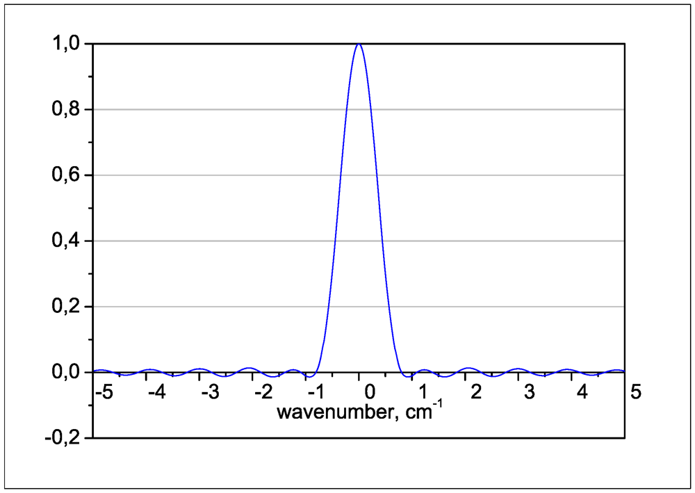
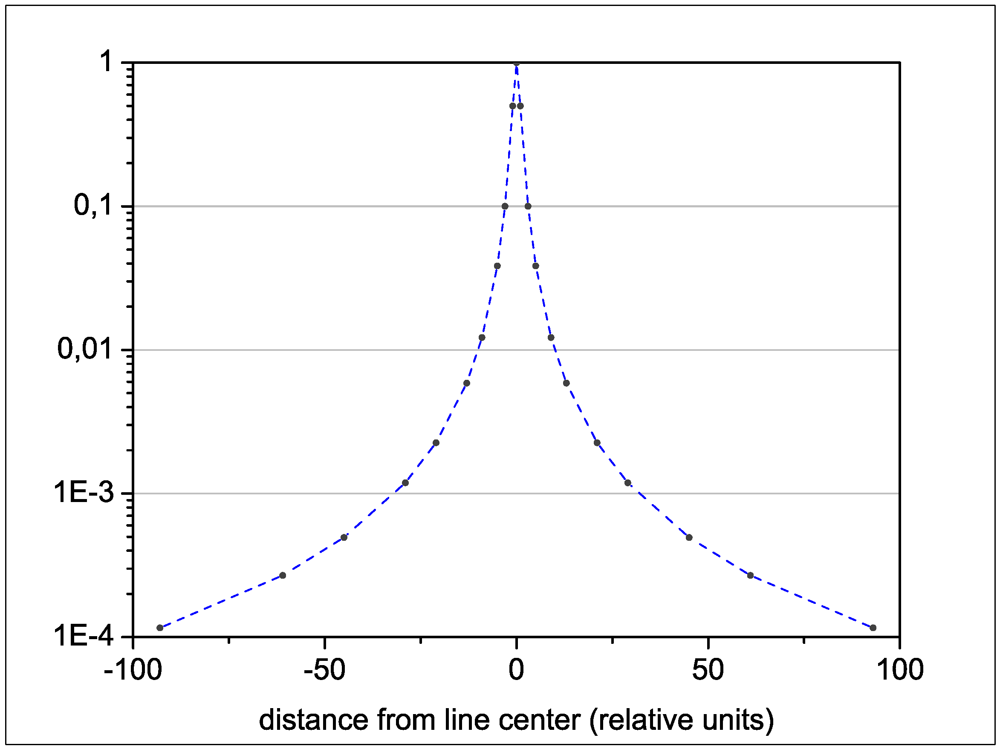
2.2. Computation of the Molecular Spectra

The monochromatic volume absorption coefficient, K(ν), at any j-th wavenumber point νj usually can be calculated by formula
Atmosphere 03 00451 i001
where fi(ν) is the absorption profile of the i-th spectral line. As was shown above it takes to consider at least ~103–104 points νj in each spectral channel of the satellite instruments, whereas a number of functions fi(ν) may reach tens of thousands and more. Moreover the absorption profile fi (ν) depends on temperature, pressure, gas volume mixing ratio and constants associated with the i-th spectral transition. So the problem of efficient LbL algorithms is of extreme importance. In FLBLM we use the algorithm suggested in (Fomin, 1995) [17], which is one of the most effective for the Summation (1) as has been tested by Kuntz and Hopfner (1998) [18]. In these algorithms we use a set of the uniform wavenumber (frequency) grids with doubling wavenumber steps. It allows the possibility for calculating each profile fi(ν) independently of others: in detail at the line center and more rarely in the far wings as shown in Figure 3.
Usually it takes less than 100 wavenumber points to approximate each fi(ν) with the required accuracy (~1%). When all the lines are taken into account, we apply the simple (parabolic) interpolation procedure to obtain the absorption spectrum at the required ~103–104 equidistant wavenumber points. It should be stressed that the procedure is performed at once to the all spectral lines that takes negligible computer times. This algorithm thus allows for increasing the calculation speed up to ~(103–104)/100 = 10–100 times and the spectra calculations usually require less computer time than further solving of the radiative transfer equations. Finally it should be mentioned that the HITRAN-2008 spectral database (Rothman et al., 2009) [19] is used for the line profile calculation as well as the MT_CKD-2.5 water vapor and other continuum models from the Line-by-Line Radiative Transfer Model (LBLRTM) (Clough, 2005) [20].
Figure 3. Illustration of the effective interpolation technique using the nonuniform wavenumber grid for the line profile calculation.
Atmosphere 03 00451 g003
In this version, photon’s trajectories are obtained by MC for scattering but non absorbing medium. The selective gas absorption is then taken into account with the help of the photon’s “weight”:
Atmosphere 03 00451 i002
where M* is the trajectory’s point and uν(M*) is the photon’s optical path. Due to the above effective LbL technique the consideration of the gaseous absorption usually needs less computer time than the MC calculations so that it is not necessary to apply the K-distribution technique.

2.3. Applied MC Technique

The scalar version of the model is a usual forward MC (Marchuk et al., 1980) [21], (Evans and Marshak, 2005) [22] combined with the LbL technique. It has been developed as long ago as in the 1990s (Fomin, et al., 1993) [23]. We will now describe the polarized version, which can calculate the Stokes vector S = (I, Q, U, V) (Chandrasekhar, 1960) [24]. The applied technique is based on the “local estimation” MC and follows the technique that has been described in detail in a paper by Cornet et al. (2010) [16]. There are two differences in the vector approach compared to the scalar one. The first difference is related to the fact that the scattering azimuth angle of a photon now is not a uniformly distributed random value between 0° and 180° degrees but depends on the initial polarization state and the scattering zenith angle. To overcome this difficulty we applied an algorithm suggested by Cornet et al. (2010) [16]. The second difficulty is related to the fact that the scattering plane rotates after each scattering so that it takes to perform a pair of rotations between the meridian and this planes. Here we follow method described in (Sushkevich, 2005) [0].
In FLBLM these monochromatic MC algorithms for the scattering but non absorbing media were combined with the above LbL algorithms to take into account the particulate and gaseous absorption by means of the photon “weights” (see (Marchuk et al., 1980), (Evans and Marshak, 2005)) [21,22]. The presented model is based on the “local estimation” MC because it allows reducing the statistical errors in calculated radiances and consequently this method is more effective for applications in the remote sensing problems.
To perform computations for any spectral regions (e.g., the instrument channels) we use two methods. In the first method, photons are uniformly distributed (usually randomly) over the given spectral region. This method has been used for a long time in the scalar version and was found very effective for calculations in the wide spectral regions due to statistical errors in each wavenumber points, which have a tendency to annihilate each other. Thus the final errors mostly depend on the total number of photons. The second method (Romanov et al., 1991) [26] wherein the same group of the photon’s trajectories (in nonabsorbing media) is used at each wavenumber point is more suitable for the very high-resolution computations: e.g., spectra themselves. Both methods are demonstrated in Figure 4, wherein a spectrum of the normalized Q-parameter at the zenith angle = 50° is shown.
In our model the cloud and aerosol optical properties are constant in the spectral range no wider than 10 cm−1 (calculation is performed in such intervals). For the next interval these optical properties are recalculated. Here we use the fact that the optical properties of aerosol and cloud vary much more smoothly compared to selective gas absorption. It should be stressed that the first method is more rapid in practical calculations and we will discuss it further in Section 4.
Figure 4. Spectra of the normalized Q-parameter at the zenith angle = 50° calculated by the first (light line) and second methods (dark line) (see text).
Atmosphere 03 00451 g004
For these calculations we used the aerosol model from the recent intercomparison with benchmark results (Kokhanovsky et al., 2010) [9] (see Section 3). The molecular scattering is also taken into account at λ ~ 0.76 μm (to illustrate situation in the A-band O2), which is comparable with the aerosol scattering at the given angle. Also we used the standard “mid-latitude summer” atmospheric model with the homogeneous aerosol layers between 0.0 and 1.0 km above the underlying surface. The spectral region is a part of the A-band O2, which is rather popular in the remote sensing.

3. Validations against Benchmark Results

The update of the model (solution of the vector radiative transfer equations) was carefully validated by means of the benchmark computations of SCIATRAN from a recent intercomparison of the vector radiative transfer codes (Kokhanovsky et al., 2010) [9]. So we use the same cloud and aerosol models that have been applied in (Kokhanovsky et al., 2010) [9]. In both models the radii a of particles follow the lognormal distributions
Atmosphere 03 00451 i003
where a0 = 0.3 μm and a0 = 5 μm, s = 0.92 and s = 0.4 for the aerosol and cloud models, respectively. It was also assumed that all these aerosol and cloud particles are nonabsorbing but refractive and their refractive indexes are 1.385 and 1.339, respectively.
Unfortunately, the “local estimation” MC mentioned above still requires a lot of computer time in a case of strong forward scattering of large particles. To overcome this difficulty we applied a usual trick: cutting-off a strong forward (diffraction) peak to smooth the phase matrix elements and then appropriate correction (decreasing) the scattering coefficients. It means disregarding scattering within small angles (~1°). Both the aerosol and cloud phase functions are shown in Figure 5(a,b).
Figure 5. Phase functions of the aerosol (a) and cloud (b) models used in this work: initial (from (Kokhanovsky et al., 2010) [9]) and after cutting-off a strong forward peak.
Atmosphere 03 00451 g005
These figures show the transformed phase functions after smoothing of the phase matrix elements and their normalization. Finally, it should be noted that in the benchmark calculations the optical thicknesses of the aerosol and cloud layers were assumed to be equal to 0.3262 and 5.0, respectively. In the case of application in our calculations of the transformed (smoothed) matrix elements the aerosol and cloud optical thicknesses have been decreased to 0.3262 × 0.95216 = 0.31088 and 5.0 × 0.68252 = 3.4126 values. The factors of 0.95216 and 0.68252 have been obtained during normalization of the phase matrix elements just after the above correction.
Results show rather good agreement with the benchmark computations; some of them are presented below. Calculations have been performed for the homogeneous nonabsorbing atmosphere and the black underlying surface. The molecular scattering has been excluded. In these calculations the solar zenith angle (SZA) and the relative azimuth between line of sight and the initial solar beam are equal to 60° and 180°, respectively. For comparison with the benchmark calculations the Stokes parameters have been normalized by factor (π/(cos(60°) × solar irradiance)). Figure 6 demonstrates an example comparison of Q-parameter in transmitted light for aerosol case (initial matrix) for different relative azimuths. Figure 7 shows the advantage of transformed matrix over the initial one for cloud model. For both these figures we used 105 photons.
Figure 6. The normalized-Q-parameter of the Stokes vector (line—SCIATRAN, circles—Fast Line-by-Line Model (FLBLM)) in transmitted light for aerosol case and initial matrix. The number of photons is 105. Relative azimuths are 0°, 90°, and 180°. Azimuths counter clock-wise.
Atmosphere 03 00451 g006
Figure 7. The normalized -Q-parameter of the Stokes vector (line—SCIATRAN, circles—FLBLM) in reflected light for cloud case. The number of photons is 105. Relative azimuths are 0°, 90°, and 180°. Azimuths counter clock-wise.
Atmosphere 03 00451 g007
Figure 8. The normalized intensity calculated for the aerosol model. Optical thickness = 0.3262, SZA = 60°, relative azimuth = 180°. Red solid line—benchmark calculations, blue dashed line—calculations using 105 photons with the transformed scattering matrix, gray dashed-dotted and green dashed lines—calculations using 104 photons with the initial and transformed scattering matrixes, respectively.
Atmosphere 03 00451 g008
Figure 9. The normalized -Q-parameter calculated for the cloud model. Optical thickness = 5.0, SZA = 60°, relative azimuth = 180°. Red solid line—benchmark calculations, blue dashed and gray dashed-dotted lines—calculations using 105 photons with the transformed and initial scattering matrixes, respectively.
Atmosphere 03 00451 g009
Besides the calculations with modified phase matrices, one of the most important things to vary is the number of photons. Some results of computations of solar radiation reflected from the above aerosol and cloud layers are shown in Figure 8 and Figure 9, respectively. These figures also demonstrate usefulness of the above cutting-off of the forward peak in the scattering matrix elements. We have performed several calculations using 104 and 105 photons for the initial and transformed scattering matrices (see Figure 8). As one can see, this trick helps to decrease number of photons in 10–100 times. It gives a hope that ~104–105 photons will be enough to reach accuracy needed for the most practical applications. (There have been used 108 photons in the benchmark calculations (Kokhanovsky et al., 2010) [9]).

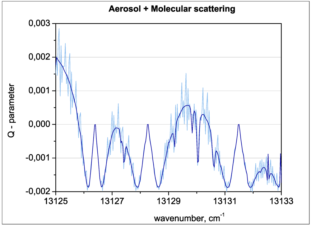
4. Application to Remote Sensing

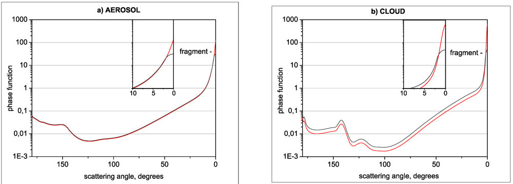
4.1. Retrieval of the Structure of Clouds and Aerosols

A measured high-resolution spectrum represents N experimental values that make it possible to evaluate J retrieval values. It should be stressed that J << N due to experimental errors and a fact that the “inverse” problem is ill-conditioned in many practical situations. Also J << N because of the statistical errors in the N measurements as well as several points contain identical information about clouds and aerosols.
Figure 10. Differences in a spectrum of the reflected solar radiation caused by change in the aerosol structure. The same that Figure 8 (the single aerosol layer between 0–1 km, optical thickness = 0.3262, Mid-Latitude Atmospheric model)but in the spectral region of the Ω—band H2O (1.87 μm). Red line – for the above homogeneous aerosol layer and blue line—for a layer of the same optical thickness but with linear dependence on altitude of the volume scattering coefficient from maximal at the surface to zero at 1 km.
Atmosphere 03 00451 g010
From high-resolution spectra of Stokes parameters measured in the molecular absorption bands of the reflected solar radiation, it should be possible to obtain several parameters describing the cloud and aerosol structures. This statement is confirmed by Figure 10, which demonstrates clearly distinguishable differences in a spectrum of the reflected solar radiation caused by changes in the aerosol structure only. The reason of the difference between homogeneous aerosol layer and a layer with extinction coefficient increasing from the top to the bottom is obvious. Indeed, the first layers near the top are more reflective leading to a weaker absorption of the photons by the atmospheric molecules. In the same way, the differences in signals between the channels are linked to the absorption and could give information at different levels.
An important question arises in such kind of satellite experiments: how do errors in the retrieval values depend on the spectral resolution and the Signal to Noise Ratio (SNR)? To make this question clear and indirectly to evaluate applicability of our model, we considered a simple but realistic numerical experiment, which simulates investigation of aerosol structures in the boundary layer. In this experiment it is supposed that the solar and satellite zenith angles = 0.0° and the aerosol optical thickness is small enough to use the “single scattering” approximation. The spectral region and atmospheric model are the same as in Figure 10. The aerosol volume scattering coefficient ρ is defined by expression
Atmosphere 03 00451 i004
where z is altitude, the nodes zj are equidistant points from 0.0 to 1.0 km and xj are the retrieval values. Thus in our numerical experiment the signal yi (normalized intensity I, Q or U component) in each spectral point is equal to
Atmosphere 03 00451 i005
where εi is the Gaussian (normal) distributed errors with variance σ2i ~ (yi*SNR)2. The Bji coefficients are
Atmosphere 03 00451 i006
where τ ji is the molecular absorption optical depth at the zj altitude and the i-th spectral point. It should be stressed that these coefficients are realistic because have been calculated by the LbL method for the given atmospheric model. We have been performed statistical analysis using the theory of maximum likelihood estimation (Rodgers, 2000) [27] that gives a system of J linear equations for J unknown values xj:
Atmosphere 03 00451 i007
where N is a number of the spectral points. For the selected spectral region 5,600–5,800 cm−1 in our numerical experiments we have tested N = 6,400, 800 and 200 (spectral resolution = 1/32, 1/4, and 1 cm−1) and J = 3, 4… Statistical errors of the xj-values, which are related to experimental errors εi, can be evaluated using the Fisher information matrix (Rodgers, 2000) [27] or by means of the series of L repetitions of the experiment. We chose the second method as more universal, wherein we have selected L = 1,000 repetitions. In each l-th repetition yi(l) have been obtained by Formula (5), where initial values <xj> = 0.1 × 2/[J(J + 1)] × (J − j + 1) (it corresponds to the linear aerosol profile with optical thickness = 0.1). Errors εi(l) have been obtained using a program that independently generates the normally distributed quantities (the diagonal covariance matrix of yi is supposed). Thus in each l-th “retrieval” (l =1, 2, …, L) we have obtained xj(l) values for the statistical data processing. The result is shown in Table 1, where relative errors in percent ηj for the xj values are calculated by expression
Atmosphere 03 00451 i008
Table 1. Relative errors (%) in a case of four retrieval values in the numerical experiment that simulates investigation of aerosol structures in the boundary layer (see text). X—the retrieved value and N—the number of spectral measurements.
X1 = 0.04X2 = 0.03X3 = 0.02X4 = 0.01
SNRN = 6,400800200N = 6,400800200N = 6,400800200N = 6,400800200
1,0001.75105 16307214051630
333515301647912164121164889
1001752102531563057121340253160297
These preliminary results confirm that retrieval of the aerosol structure by the discussed method is possible even in the thin boundary layer. However, it needs to take into account spectra consisting from thousands of the spectral points and SNR must be greater than ~300 (as in TANSO-FTS). Also it can be expected that number of the independent parameters (degree of freedom) hardly exceeds J = 3–4 for real instruments.
As a whole errors ηj, as was expected, are inversely proportional to a factor SNR*(N)0.5. So it may seem that it is the same to use different spectral resolutions and spectral intervals if only the number of points N is the same. In Table 2, we have tested the effect of the spectral resolution on the relative error by keeping the number of spectral points to N = 200 and repeated our experiment in the spectral regions 6,200–6,206.25 cm−1 and 6,200–6,400 cm−1 with spectral resolutions 1/32 cm−1 and 1 cm−1, respectively.
Table 2. The same that Table 1 but for spectral resolutions are 1/32 and 1.0 cm−1 and spectral regions are 6,200–6,206.5 and 6,200–6,400, respectively. The number of the spectral points N = 200.
X1=0.04X2=0.03X3=0.02X4=0.01
SNR1/32 1.01/32 1.0.1/32 1.0.1/32 1.0
1,0007.91020 3021401430
33324305991631214189
10079102196305211402137297
As one can see errors in the high-resolution retrieval are essentially less than in other case and, consequently, the high-resolution measurements are preferable: evidently because they can better use more informative parts of a spectrum. Also it should be mentioned that measurements of the Q and U components of the Stokes vector allow better investigation of aerosols and clouds because they often are the main polarizing factor. Thus the high-resolution polarized measurements seem rather promising.

4.2. Time Considerations for High Resolution Spectra Calculations

To investigate applicability of the model to remote sensing as a “forward” model we have performed some numerical experiments with an imagined hybrid of POLDER and TANSO-FTS. The result was a simulation of the measurements by FTS with the spectral resolution equals to 0.5 cm−1 (see Figure 1) in a band 13,000–13,200 cm−1. In this section we present some computer time estimations for calculation of simulated spectra measurements. It took ~10 hours for the calculations performed by the second method (see Section 2.3) using an ordinary computer (CPU 3.20 GHz) with a spectral resolution equal to 1/32 = 0.03125 cm−1 in the spectral region 13,000–13,200 cm−1 (the POLDER’s channel 768.35–757.45 nm) for a triplet of the relative azimuth angles (0, 90 and 180 degrees) and ten of the zenith angles (0, 10, 20 … 90 degrees). The number of photons was 2,000,000 in each 8.0 cm−1 spectral subinterval, where the scattering properties are supposed constant. But the number of photons can be essentially decreased if we apply the more rapid first method. It took only 20,000 instead of 2,000,000 photons and ~10 minutes of the computer time. Figure 11 demonstrates the initial and convoluted spectra obtained by the both methods for the aerosol layer between 0 and 1 km.
Figure 11. Initial (blue line) and convoluted with the response function (Figure 1) (red and gray lines) spectra of the normalized Q-parameter in the standard “Mid-latitude Summer Atmosphere”. The homogeneous aerosol layer is between 0–1 km. Solid blue line—initial spectrum; red solid line and dashed gray lines—convoluted spectra obtained by the second method using 2 × 10⁶ and first method using 2 × 10⁴ photons, respectively.
Atmosphere 03 00451 g011
Nevertheless the visible statistical errors are less than the spectrum distortion because of the convolution. It should be noted that these errors become practically invisible for ~100,000 photons and it takes ~1 hour of the computer time. Due to the fact that the statistical errors mostly depend on the total number of photons (not spectral interval) the computer time is inversely proportional to the spectral resolution. Thus calculations for POLDER need ~100 times less computer time than for TANSO-FTS (several minutes only).

5. Conclusions

The update of the presented model has been successfully validated by means of the recent intercomparison (Kokhanovsky et al., 2010) [9]. Being installed on a typical PC, FLBLM simulates high-resolution measurements (with resolution ~0.5 cm−1) in a ~100 cm−1 spectral region during ~10–100 minutes (depending on the required accuracy). It takes only several minutes to obtain results for the medium resolution measurements (e.g., by POLDER, 3MI, etc.).
Our results confirm that the high-resolution spectrum of the Stokes parameters of the reflected solar radiation contain much more useful information about structures of the scattering layers than the medium-resolution one. The presented model thus seems applicable for the remote sensing as a simulator and for validations.

Acknowledgments

This work was supported by grants from RFBR (11-01-00021 and 09-01-00071).

References

  1. IPCC. Summary for Policymakers. Available online: http://www.ipcc.ch/pdf/assessment-report/ar4/wg1/ar4-wg1-spm.pdf (accessed on 15 December 2007).
  2. King, M.D.; Menzel, P.W.; Kaufman, Y.J.; Tanre, D.; Gao, B.C.; Platnick, S.; Ackerman, S.A.; Remer, L.A.; Pincus, R.; Hubanks, P.A. Cloud and aerosol properties, precipitable water, profiles of temperature and water vapor from MODIS. IEEE Trans. Geosci. Remote Sens. 2003, 41, 442–458. [Google Scholar] [CrossRef]
  3. Bizzari, B. The space-based global observing system in 2011 (GOS-2011). Available online: ftp://ftp.wmo.int/Documents/PublicWeb/sat/DossierGOS (accessed on 1 September 2011).
  4. Chang, F.L.; Li, Z. Estimating the vertical variation of cloud droplet effective radius using multispectral near-infrared satellite measurements. J. Geophys. Res. 2002, 107, 1–12. [Google Scholar]
  5. Fisher, J.; Grassl, H. Detection of cloud top-height from backscattered radiances within the oxygen A-band. Part 1: Theoretical study. J. Appl. Meteorol. 1991, 30, 1245–1259. [Google Scholar] [CrossRef]
  6. Kokhanovsky, A.A. Reference. In Cloud Optics; Springer: Berlin, Germany, 2006. [Google Scholar]
  7. Liou, K.N.; Goody, R.M.; West, R. CIRRUS: A Low Cost Cloud/Climate Mission. Office of Space Science NASA: Washington, DC, USA, 1996. [Google Scholar]
  8. Mishchenko, M.I.; Hovenier, J.W.; Travis, L.D. Reference. In Light Scattering by Nonspherical Particles; Academic Press: San Diego, CA, USA, 2000. [Google Scholar]
  9. Kokhanovsky, A.A.; Budak, V.P.; Cornet, C.; Duan, M.; Emde, C.; Katsev, I.L.; Klyukov, D.A.; Korkin, S.V.; C-Labonnote, L.; Mayer, B.; Min, Q.; Nakajima, T.; Ota, Y.; Prikhach, A.S.; Rozanov, V.V.; Yokota, T.; Zege, E.P. Benchmark results in vector atmospheric radiative transfer. J. Quant. Spectrosc. Rad. Transfer. 2010, 111, 1931–1946. [Google Scholar] [CrossRef]
  10. Fomin, B.A.; Correa, M.P. A k-distribution technique for radiative transfer simulation in inhomogeneous atmosphere: 2. FKDM, fast k-distribution model for the shortwave. J. Geophys. Res. 2005. [Google Scholar] [CrossRef]
  11. Tarasova, T.A.; Fomin, B.A. The use of new parameterizations for gaseous absorption in the CLIRAD-SW solar radiation code for models. J. Atmos. Ocean. Technol. 2007, 24, 1157–1163. [Google Scholar] [CrossRef]
  12. Fomin, B.A.; Mazin, I.P. Model for an investigation of radiative transfer in cloudy atmosphere. Atmos. Res. 1998. [Google Scholar] [CrossRef]
  13. Halthore, R.N.; Crisp, D.; Schwartz, S.E.; Anderson, G.P.; Berk, A.; Bonnel, B.; Boucher, O.; Chang, F.-L.; Chou, M.-D.; Clothiax, E.E.; Dubuisson, P.; Fomin, B.; Fouquart, Y.; Freidenreich, S.; Gautier, C.; Kato, S.; Lazlo, I.; Li, Z.; Plana-Fattori, A.; Ramaswamy, V.; Ricchiazzi, P.; Shiren, Y.; Trischenko, A.; Wiscombe, W. Intercomparison of shortwave radiative transfer codes and measurements. J. Geophys. Res. 2005. [Google Scholar] [CrossRef]
  14. Forster, P.; Fomichev, V.; Rozanov, E.; Cagnazzo, C.; Jonsson, A.; Langematz, U.; Fomin, B.; Iacono, M.; Mayer, B.; Mlawer, E.; Myhre, G.; Portmann, R.; Akiyoshi, H.; Falaleeva, V.; Gillett, N.; Karpechko, A.; Li, J.; Lemennais, P.; Morgenstern, O.; Oberländer, S.; Sigmond, M.; Shibata, K. Evaluation of radiation scheme performance within chemistry climate models. J. Geophys. Res. 2011. [Google Scholar] [CrossRef]
  15. Oreopulos, L.; Mlawer, E.; Delamere, J.; Shippert, T.; Cole, J.; Fomin, B.; Iacono, M.; Jin, Z.; Manners, J.; Raisanen, P.; Rose, F.; Zhang, Y.; Wilson, M.; Rossow, W. The continual intercomparison of radiation codes: Results from phase I. J. Geophys.Res. 2012. [Google Scholar] [CrossRef]
  16. Cornet, C.; C-Labonnote, L.; Szcap, F. Three-dimensional polarized Monte Carlo atmospheric radiative transfer model (3DMCPOL): 3D effects on polarized visible reflectances of a cirrus cloud. J. Quant. Spectrosc. Rad. Transfer. 2010, 111, 174–186. [Google Scholar] [CrossRef]
  17. Fomin, B.A. Effective interpolation technique for line-by-line calculations of radiation absorption in gases. J. Quant. Spectrosc. Rad. Transfer. 1995, 53, 663–669. [Google Scholar] [CrossRef]
  18. Kuntz, M.; Hopfner, M. Efficient line-by-line calculation of absorbing coefficients. J. Quant. Spectrosc. Rad. Transfer. 1999, 110, 97–104. [Google Scholar] [CrossRef]
  19. Rothman, L.S.; Gordon, I. E.; Barbe, A.; Benner, D.C.; Bernath, P.F.; Birk, M.; Boudon, V.; Brown, L.R.; Campargue, A.; Champion, J.-P.; Chance, K.; Coudert, L.H.; Dana, V.; Devi, V.M.; Fally, S.; Flaud, J.-M.; Gamache, R.R.; Goldman, A.; Jacquemart, D.; Kleiner, I.; Lacome, N.; Lafferty, W.J.; Mandin, J.-Y.; Massie, S.T.; Mikhailenko, S.N.; Miller, C.E.; Moazzen-Ahmadi, N.; Naumenko, O.V.; Nikitin, A.V.; Orphal, J.; Perevalov, V.I.; Perrin, A.; Predoi-Cross, A.; Rinsland, C.P.; Rotger, M.; Šimečková, M.; Smith, M.A.H.; Sung, K.; Tashkun, S.A.; Tennyson, J.; Toth, R.A.; Vandaele, A.C.; Vander Auwera, J. The HITRAN 2008 molecular spectroscopic database. J. Quant. Spectrosc. Rad. Transfer. 2009, 110, 533–572. [Google Scholar]
  20. Clough, S.A.; Shepard, M.W.; Mlawer, E.J.; Delamere, J.S.; Jacono, M.J.; Cady-Pereira, K.; Boukabara, S.; Brown, P.D. Atmospheric radiative transfer modeling: A summary of the AER codes. J. Quant. Spectrosc. Rad. Transfer. 2005, 91, 233–244. [Google Scholar] [CrossRef]
  21. Marchuk, G.I.; Mikhailov, G.A.; Nazaraliev, M.A.; Darbijan, R.A.; Kargin, B.A.; Elepov, B.S. Reference. In The Monte Carlo Method in Atmospheric Optics; Springer: New York, NY, USA, 1980. [Google Scholar]
  22. Evans, K.F.; Marshak, A. Numerical Methods. In 3D Radiative Transfer in Cloudy Atmospheres; Springer: Berlin, Germany, 2005. [Google Scholar]
  23. Fomin, B.A.; Rublev, A.N.; Trotsenko, A.N. Line-by-line Procedures to Compute Radiative Transfer Parameters in Scattering Atmosphere. In Proceeding of IRS’92: Current Problems in Atmospheric Radiation. A.DEEPAK Publishing: Hampton, VA, USA, 1993. [Google Scholar]
  24. Chandrasekhar, S. Reference. In Radiative Transfer; Dover: New York, NY, USA, 1960. [Google Scholar]
  25. Sushkevich, T.A. Reference. In Mathematical Models of Radiation Transfer; BINOM: Moscow, Russia, 2005. (in Russian) [Google Scholar]
  26. Romanov, S.V.; Trotsenko, A.N.; Fomin, B.A. Reference. In Application of the Numerical Methods to Describe the Transfer of Solar Radiation in The Scattering Atmosphere with Accurate Treatment of The Selective Gas Absorption; Preprint Institute of Atomic Energy: Moscow, Russia, 1991. (in Russian) [Google Scholar]
  27. Rodgers, C.D. Reference. In Inverse Method for Atmospheric Sounding; World Scientific: River Edge, NJ, USA, 2000. [Google Scholar]

