Article

How Does a Regional Climate Model Modify the Projected Climate Change Signal of the Driving GCM: A Study over Different CORDEX Regions Using REMO

1
Climate Service Center, Helmholtz-Zentrum Geestacht, Fischertwiete 1, D-20095 Hamburg, Germany
2
Max Planck Institute for Meteorology, Bundesstreet 53, D-20146 Hamburg, Germany
*
Author to whom correspondence should be addressed.
Atmosphere 2013, 4(2), 214-236; https://doi.org/10.3390/atmos4020214
Submission received: 1 February 2013 / Revised: 20 May 2013 / Accepted: 3 June 2013 / Published: 14 June 2013

Abstract

:
Global and regional climate model simulations are frequently used for regional climate change assessments and in climate impact modeling studies. To reflect the inherent and methodological uncertainties in climate modeling, the assessment of regional climate change requires ensemble simulations from different global and regional climate model combinations. To interpret the spread of simulated results, it is useful to understand how the climate change signal is modified in the GCM-RCM modelmodelgeneral circulation model-regional climate model (GCM-RCM) chain. This kind of information can also be useful for impact modelers; for the process of experiment design and when interpreting model results. In this study, we investigate how the simulated historical and future climate of the Max-Planck-Institute earth system model (MPI-ESM) is modified by dynamic downscaling with the regional model REMO in different world regions. The historical climate simulations for 1950–2005 are driven by observed anthropogenic forcing. The climate projections are driven by projected anthropogenic forcing according to different Representative Concentration Pathways (RCPs). The global simulations are downscaled with REMO over the Coordinated Regional Climate Downscaling Experiment (CORDEX) domains Africa, Europe, South America and West Asia from 2006–2100. This unique set of simulations allows for climate type specific analysis across multiple world regions and for multi-scenarios. We used a classification of climate types by Köppen-Trewartha to define evaluation regions with certain climate conditions. A systematic comparison of near-surface temperature and precipitation simulated by the regional and the global model is done. In general, the historical time period is well represented by the GCM and the RCM. Some different biases occur in the RCM compared to the GCM as in the Amazon Basin, northern Africa and the West Asian domain. Both models project similar warming, although somewhat less so by the RCM for certain regions and climate types. A common feature in regions of tropical climate types is that REMO shows dryer climate conditions than forMax Planck Institute for Meteorology-Earth System Model (MPI-ESM) for RCP 4.5 and RCP 8.5, leading to an opposing sign in the climate change signal. With an increase in radiative forcing from RCP 2.6 to RCP 8.5 and towards the end of the 21st century, some of the detected differences between GCM and RCM are more pronounced.

1. Introduction

General circulation models (GCMs) are commonly used to assess present-day climate and possible future climate changes at the global scale at rather coarse resolutions (mostly 300 to 100 km) [1,2,3,4,5,6]. In order to investigate regional impacts of different climate conditions, spatially higher resolved information about the state of the regional climate system is needed [7,8,9,10,11]. Therefore, regional climate models (RCMs) are frequently used (e.g., [12,13,14,15]). The large scale information of the atmosphere from the GCM serves as lateral forcing for the RCM and is dynamically refined within a model domain, where the RCM is able to simulate mesoscale climate features [16,17,18]. To reflect the inherent and methodological uncertainties in climate modeling, the assessment of regional climate change requires ensemble simulations by different global and regional climate model combinations as is done in several past and present international projects, e.g., PRUDENCE [19], ENSEMBLES [20] and the COordinated Regional Climate Downscaling EXperiment (CORDEX) [21,22]. In order to help interpret the spread of the simulated results, it is useful to know how the climate change signal is modified within the individual modeling chains of global to regional models. Further, for various reasons, impact modelers may not be able to consider the full ensemble; rather they need to select a number of simulation runs representative of the full ensemble range. In this study, we analyze one specific modeling chain over different continents. We want to answer the question, how does the RCM REMO modifiesmodify the simulated historical climate and the global climate change signal of the driving GCM Max Planck Institute for Meteorology-Earth System Model (MPI-ESM). The evaluation is done for annual mean near-surface temperature and precipitation. We investigate systematic differences in the climate change signals over different domains for Africa, Europe, South America and West Asia for regions that are based on climate types as defined by Köppen-Trewartha [23]. This allows for climate type specific analysis of simulated annual mean temperature and precipitation values across multiple model domains and continents. Consistent signal differences for one climate type over different domains would be an indication that the modification is governed by climate type specific physical processes. For example, in a climate type with high precipitation rates, the signal difference could be caused by resolving higher precipitation intensities in the regional model than in the global model. Additionally, we want to address the question of whether the bias in the control period has an influence on the climate change signal. For this study, we use a similar model set-up for dynamic downscaling over different regions of the globe that are defined within CORDEX. These CORDEX domains are widely used for regional studies across the globe (e.g., [24,25,26,27,28]). The driving simulations of MPI-ESM are performed within the framework of the Coupled Model Intercomparison Project Phase 5 (CMIP5) [29], using the Representative Concentration Pathways (RCPs), which prescribe future atmospheric greenhouse gas concentrations and aerosols [30].
The paper is structured as follows: in Section 2 a description of the model and experiment setup is given. Section 3 describes the analysis method. In Section 4 results are discussed with respect to the ability of the models to represent present day climate in the control period, and with respect to the differences in the climate change signal, as projected by the global and the regional model. Finally, some conclusions are given in Section 5.

2. Model and Experiment Setup

In this study, we apply the regional climate model REMO [31,32] to downscale global simulations of the Max Planck Institute for Meteorology-Earth System Model MPI-ESM over several CORDEX domains.

2.1. MPI-ESM

The MPI-ESM consists of the general circulation model for the atmosphere ECHAM6 [33] coupled to the MPI Ocean Model (MPI-OM) [34]. The model system is further coupled to dynamic process models for marine biogeochemistry—the Hamburg Model of Ocean Carbon Cycling (HAMOCC5) [35,36] and for the land biosphere—the Jena Scheme for Biosphere-Atmosphere Coupling in Hamburg (JSBACH) [37,38]. Here, we use the experiments conducted within the frame of CMIP5 of MPI-ESM [39] in the Low Resolution (LR) configuration with the atmosphere in spectral truncation of T63 and 47 vertical levels. MPI-OM is used with a bi-polar grid at 1.5 horizontal resolution and 40 vertical levels. The main conceptual differences to the predecessor model ECHAM5/MPI-OM [40,41], which was applied in CMIP3, are the fully coupled carbon cycle and the stratosphere resolved up to 0.01 hPa.

2.2. MPI-ESM Experiments

The historical experiment of MPI-ESM started in 1850 from a pre-industrial control simulation with a total length of 1,000 years with prescribed constant natural climate forcing. Starting from three different years of the pre-industrial control run, three realizations were integrated from 1850–2005 under observed natural and anthropogenic forcings. The natural forcing considers variations of the Earth orbit, variability in spectral solar irradiance, stratospheric aerosols from volcanic eruptions and seasonally varying natural tropospheric aerosols. The anthropogenic forcing considers well-mixed greenhouse gases (CO 2 , CH 4 , N 2 O, CFC-11, CFC-12), ozone and anthropogenic sulfate aerosols, which are spatially and seasonally resolved. Anthropogenic land-cover change is modeled in JSBACH [37] based on the New Hampshire Harmonized Land Use Protocol 3 [42] for the period 1500–2100. For more details about the climate forcings see Giorgetta et al. [39]. In this study, we use the first realization from 1950–2005 for the downscaling experiments.
The global climate change experiments are initialized with the state at the end of the corresponding historical experiment. They are conducted for the period 2006–2100 following the Representative Concentration Pathway (RCP) scenarios developed by Moss et al. [43]. MPI-ESM was used for RCP 2.6 [44], RCP 4.5 [45] and RCP 8.5 [46] which prescribe the respective low, middle, and high concentrations of greenhouse gases, tropospheric ozone and tropospheric aerosols, which had been modeled for each RCP, and the anthropogenic land-use scenarios based on Hurtt et al. [42]. The natural forcing is the same as in the historical experiment, except for volcanic aerosols, which are set to zero. For each RCP experiment, again three realizations exist whereof only the first realization of each RCP experiment is used in this study corresponding to the first realization of the control period mentioned above.

2.3. REMO

For the regional downscaling experiments, the hydrostatic version of the regional model REMO2009 is used (further denoted as REMO). REMO [31,32] is a limited-area three-dimensional atmospheric circulation model. It is based on the ‘Europa-Modell’ of the German Weather service [47] and on the physical parameterizations of the global three-dimensional atmospheric circulation model ECHAM-4 [48]. Some important model specifications of REMO are listed in Table 1 [49,50,51,52,53,54,55,56,57].
Table 1. Regional model (REMO) specifications used for the COordinated Regional Climate Downscaling EXperiment (CORDEX) simulations.
Model VersionVertical Coordinates/LevelsAdvection SchemeTimestepConvection SchemeRadiation SchemeTurbulent Vertical DiffusionCloud Microphysics SchemeLand Surface Scheme
REMO2009 hydrostatichybrid / 27–31Semi-lagrangian240 sTiedtke [49], Nordeng [50], Pfeifer [51]Morcrette et al. [52], Giorgetta [53]Louis [54]Lohmann and Roeckner [55]Hagemann [56], Rechid et al. [57]
These are the same specifications as applied in Jacob et al. [28] for downscaling global reanalysis data over several CORDEX domains, with one exception for West Asia. Here, the parameter value for cloud height over land - the distance between cloud top and cloud base—that has to be reached before a cloud can rain was set to a lower value in order to improve the representation of precipitation in this region. Additionally, the model parameterization differs from the version used in all other domains in West Asia, which was not discussed in Jacob et al. [28]. It has to be kept in mind for the interpretation of the results, that the soil heat conductivity was reduced by applying values that are representative for dry soils, which was found to be more appropriate over large parts of India (refer to Kumar et al. [58]).

2.4. REMO Experiments

The first realization of the MPI-ESM historical experiment and of the RCP 2.6, RCP 4.5 and RCP 8.5 experiments are downscaled with REMO to the CORDEX domains for Africa, Europe, South America, and West Asia. The historical experiments are downscaled for 1950–2005 and the RCP experiments for 2006–2100. The global data is prescribed at the lateral boundaries of each CORDEX domain with an exponential decrease towards the inner model domain. The main direct influence of the boundary data lies in the eight outer grid boxes using a relaxation scheme according to Davies [59]. The horizontal target resolution is 0.44 on a regular grid, and the vertical atmosphere contains 27 or 31 levels on a hybrid vertical coordinate system (refer to Table 1). The time series of the observed greenhouse gas concentrations are prescribed to the regional historical simulation. The time series of the projected greenhouse gas concentrations are prescribed to the respective regional RCP experiment. Other anthropogenic and natural forcings such as ozone and aerosols (refer to Tanré et al. [60]) are kept constant. As is frequently done in regional climate modeling studies, land cover change is not considered due to the lack of high resolution datasets. Large scale climate information is transported into the model domain via the lateral boundaries as well as via the sea surface temperatures at the lower boundary.

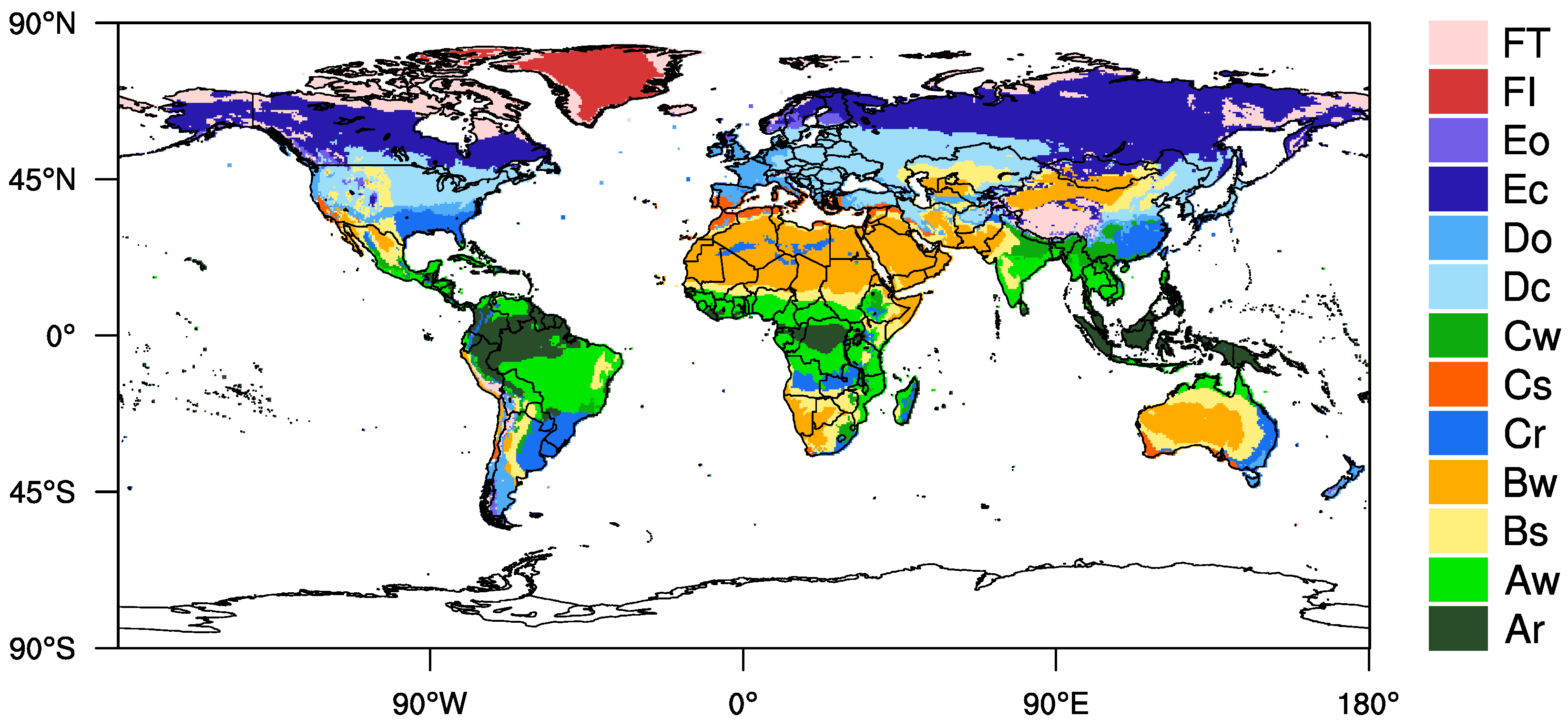
3. Analysis Methodology

The simulations for the historical time period are analyzed with respect to the ability of the global and the regional model to represent present-day climate.
The 30-year time period from 1971–2000 is analyzed and also serves as a reference for the future climate change simulations. The analyzed future time periods extend from 2036–2065 for the mid-century and from 2071–2100 for the end of the century. The climate change signals can be defined as the differences in the climatological mean values of the the future to the reference time period.
We calculate the climatological mean values over the 30-year time period as follows. For horizontal plots, the temporal mean per grid box is calculated. For overlapping regions (mainly Europe, Africa and West Asia), we applied masks in order to only use values that belong to the respective geographical continent for each CORDEX domain. Within Section 4, we additionally discuss the results in these overlapping regions. In order to investigate differences in the climate change signal independent of the model domain, we calculate mean values over different continent independent areas following the climate type classification of Köppen-Trewartha [23], as listed in Table 2 ([61,62]). Regions of the same Köppen-Trewartha climate type are calculated using version 3.0 of the Climate Research Unit (CRU) observational dataset [63] (denoted as CRU in the following) and are fixed in this study. Areas corresponding to the different climate types are shown in Figure 1. CRU data also serve as reference for the representation of present-day climate. For comparison, model data are remapped to the regular global 0.5 × 0.5 grid of the CRU data using conservative remapping, that is first order area weighted remapping.
Table 2. Köppen-Trewartha (K-T) climate types based on Trewartha and Horn [61]. Table was taken and edited from Castro et al. [62].
ClimateKöppen-TrewarthaDefinition
Tropical humidArAll months above 18 C and less than 3 dry months
Tropical wet-dryAwSame as Ar, but 3 or more dry months
Dry aridBWAnnual precipitation P (in cm) smaller, or equall to 0 . 5 × A
Dry semi-aridBSAnnual precipitation P (in cm), greater than 0 . 5 × A
Subtropical summer-dryCs8–12 months above 10 C , annual rainfall less than 89 cm and dry summer
Subtropical summer-wetCwSame thermal criteria as Cs, but dry winter
Subtropical humidCrSame as Cw, with no dry season
Temperate oceanicDo4–7 months above 10 C and the coldest month above 0 C
Temperate continentalDc4–7 months above 10 C and the coldest month below 0 C
Sub-arctic oceanicEoUp to 3 months above 10 C and the coldest month above −10 C
Sub-arctic continentalEcUp to 3 months above 10 C and the coldest month below or equal to −10 C
Tundra/HighlandFTAll months below 10 C
Ice capFIAll months below 0 C
Figure 1. Köppen-Trewartha (K-T) climate types. The derived Köppen-Trewartha (K-T) climate classification based on the 30-year mean of the CRU dataset: FT (tundra/highland), FI (ice cap), Eo (sub-arctic oceanic), Ec (sub-arctic continental), Do (temperate oceanic), Dc (temperate continental), Cw (subtropical summer-wet), Cs (subtropical summer-dry), Cr (subtropical humid), BW (dry arid), BS (dry semi-arid), Aw (tropical wet-dry), Ar (tropical humid) see also Table 2.
Atmosphere 04 00214 g001
Temperature values are height corrected using a lapse rate of 0.0064 K/m in order to take into account the differences between the orographies of CRU, the global and the regional model. In a subsequent step, masks for the different climate types are applied for the different domains. Climate types that cover less than 5% of the land area of a model domain are excluded from the analysis. Values for temperature and precipitation are then compared for the same climate type in different regions. Using this method, features depending on a distinct climate type can be distinguished from features depending on a model domain. Here we analyze only annual means due to the different timing of seasons within climate types, which are present in the northern and southern hemisphere or on different continents. A detailed analysis of seasonal cycles applying a different evaluation methodology taking into account the different timing of seasons and climatic conditions will be done in a future study.

4. Results and Discussion

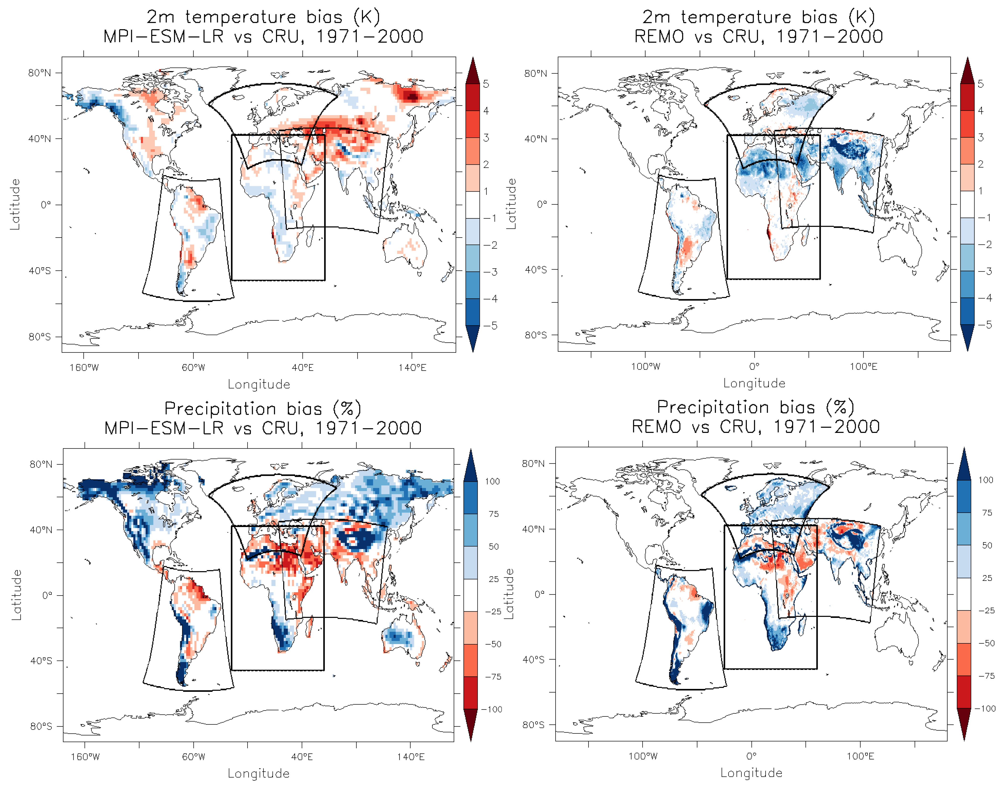
4.1. Evaluation of the Simulated Historical Climate

This chapter describes the performance of the two models in representing the present day climate within the reference period 1971–2000. The differences to the observational dataset of CRU v3.0 for 30 year annual means for temperature and precipitation are analyzed. They are shown in Figure 2. The top row shows the temperature bias, while the bottom row shows the precipitation bias as relative difference. On the left hand side, the results for MPI-ESM are shown and on the right hand side, the corresponding downscaled results of REMO.

4.1.1. Temperature

Generally, REMO results are cooler than MPI-ESM results. MPI-ESM has a prominent warm bias from Southern Europe to Central Asia of at least 2 K, as can be observed in the upper left panel in Figure 2. In contrast, REMO has a cold bias for the Sahara region and the entire West Asian domain shown in the upper right panel in Figure 2. The largest difference of REMO to CRU v3.0 is in the Tibetan Plateau where, however, the quality of the CRU observations is questionable due to the lack of observations.
For most parts of Africa, apart from the Sahara region, both models show minor temperature biases of less than 2 K, except for a common warm bias in a narrow band along the region of the Benguela upwelling system, located off the coast of South-West Africa.
For South America, temperature biases of the regional and the global simulation are rather similar, with warm biases up to 2 K over the Amazon Basin and Patagonia. An existing Amazonian warm bias in predecessor simulations was substantially reduced as described in Jacob et al. [28], by prescribing more realistic values for the water holding capacity of tropical forests in this region, which are characterized by large rooting depths [64].
There are two regions in which the model domains overlap considerably: The northern part of the African domain overlaps the European domain and the northeastern part of the African domain overlaps the West Asian domain. Comparing temperature biases inside the overlapping regions, the Africa/Europe region shows a very similar pattern and magnitude of the biases. In the Africa/West Asia region, the bias patterns are similar in both domains, while the cold bias versus CRU is more pronounced (by about 1–3 K) in the West Asia domain (not shown).
Figure 2. Historical time period compared with CRU, annual mean 2m-temperature and annual precipitation sums. The temperature difference is plotted in K in the upper panels for the historical time period as simulated by the Earth system model MPI-ESM (LR) (left panel) and REMO (right panel). Precipitation differences are plotted in mm/day in the lower panels as simulated by the Earth system model MPI-ESM (LR) (left panel) and REMO (right panel) compared to observational data of CRU.
Atmosphere 04 00214 g002

4.1.2. Precipitation

In general, the patterns of the precipitation biases (shown in the lower panels in Figure 2) look rather similar for both models, although differences can be seen in the magnitudes. One has to keep in mind that the relative difference overemphasizes the bias in areas with low precipitation.
A consistent wet bias between 25%–50% can be seen over Europe. A strong common wet bias is seen on the west coast of South America, as well as for the west coast of Africa. In the coastal region of the Amazon Basin, MPI-ESM shows a dry bias which is reduced by REMO, while the wet bias in the eastern parts of South America is increased. While MPI-ESM has a dry bias for central to southern India, REMO simulates a wet bias for these areas.
The bias in the overlapping region of Africa and Europe shows again the same pattern and magnitude. In the Africa/West Asia overlapping region, the pattern is similar, while the magnitude shows differences of about 25 percentage points in some regions (not shown).

4.1.3. Discussion

Except for temperature in the subtropical band of the Northern hemisphere and Central Asia, the patterns for both temperature and precipitation are similar.
The cold bias over the Sahara region was already present in the ERA-Interim driven hindcast simulation and seems to be a REMO feature. However it is difficult to quantify the cold bias, as it is a region extremely sparse with observations. It could be related to less incoming shortwave radiation over the Sahara region compared to MPI-ESM. One possible reason for this is the comparatively high aerosol optical depth of the the aerosol climatology by Tanré et al. [60] used in the regional model as shown for a European domain by Zubler et al. [65].
To investigate why REMO cools down the MPI-ESM results for the West Asian domain substantially, we compared the atmospheric driving fields of MPI-ESM with the corresponding fields in REMO. The mean seasonal circulation is not substantially altered by REMO, indicating that it is mainly determined by the lateral GCM-forcing and, to a minor extent by the internal freedom of REMO in the center of the domain, (e.g., [66]). There are only minor temperature differences between MPI-ESM and REMO in the lower troposphere at 850 hPa. The small temperature differences indicate that the different surface and soil schemes in the two models generate the difference in the near surface temperature. The different thermal conductivities used for the domains are supposed to be one of the reasons for the cooling. Nevertheless, this is in contrast to former studies performed under the HighNoon project using ECHAM5 and the Hadley Center as driving model where we could not find a cold bias in the region, although we used modified soils.
Concerning precipitation, the pattern may be affected by a cold bias in the sea surface temperature (SST) simulated by MPI-ESM compared to ERA-Interim in the Indian ocean. Especially over the Arabian Sea, the bias is on the order of 2 K. Since the South Asian climate is strongly dependent on the air sea interaction [67], this bias significantly influences the local climate. For a sensitivity experiment, in which the MPI-ESM simulated SST was replaced by the SST of ERA-Interim, the results indicate that the monsoon precipitation is better simulated with the corrected SST. However, the changed SST did not affect the temperature over land substantially.
Further investigations of the reasons for the substantial differences in temperature are of interest, but are not within the scope of this paper.
The Africa/Europe overlapping region shows that the bias versus CRU is not altered by the choice of the model domain. Boundary conditions and local processes have similar influences inside this region. This seems to be different for the Africa/West Asia region, where differences in the bias are detected. One possible explanation is the difference in coverage of inflow areas by the regional models: Africa and Europe have a similar western boundary in the Africa/Europe overlapping region and thus also similar western boundary conditions (the main inflow in this region). The advection pattern in the Africa/West Asia overlapping region is more complex. Air masses advected over the African continent are resolved by the regional model over the Africa domain while air masses advected over the Indian ocean are better represented by the West Asian domain. To some extent the different temperature biases in the Africa and West Asia domains can be related to different soil heat conductivities (refer to Section 2.3).

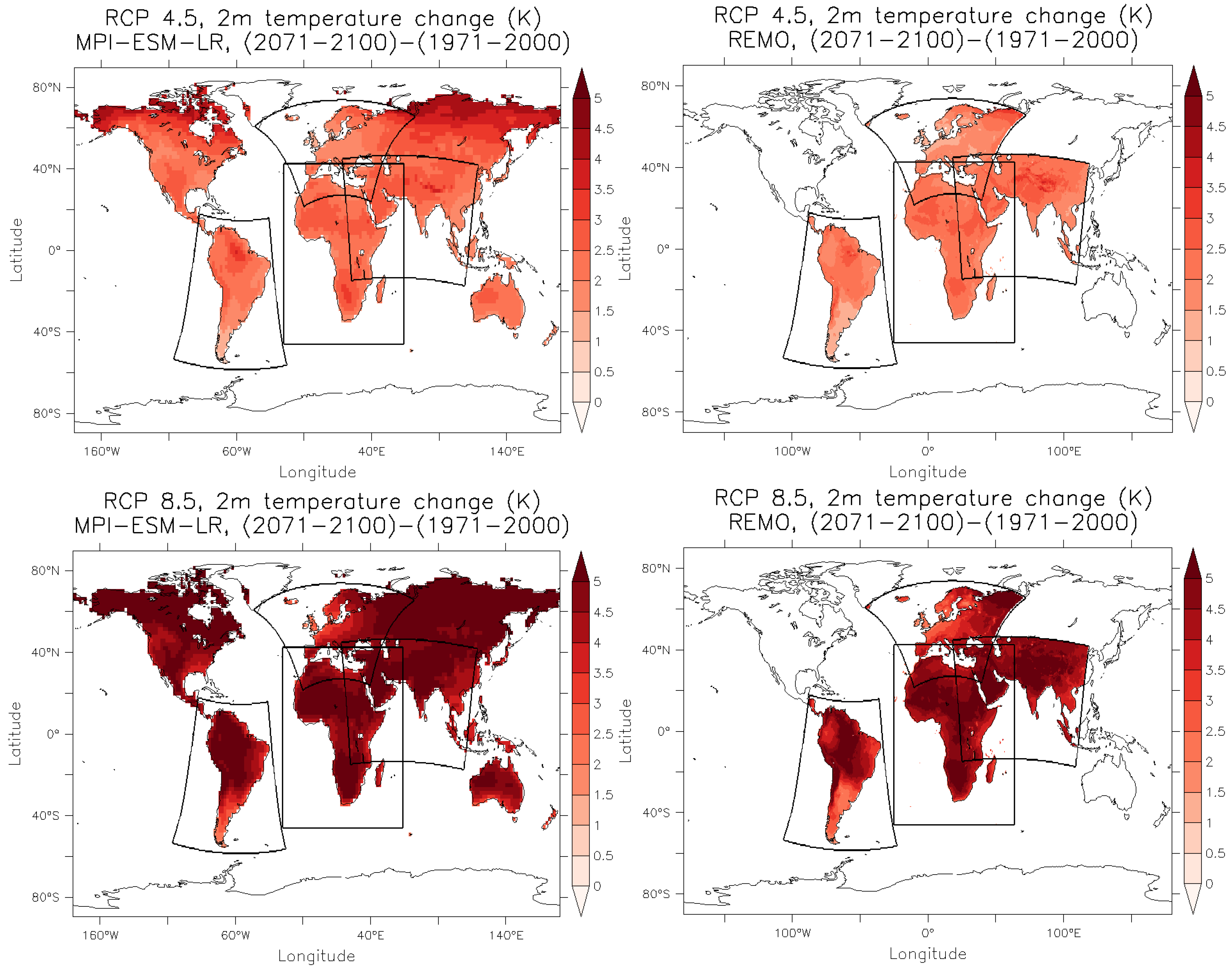
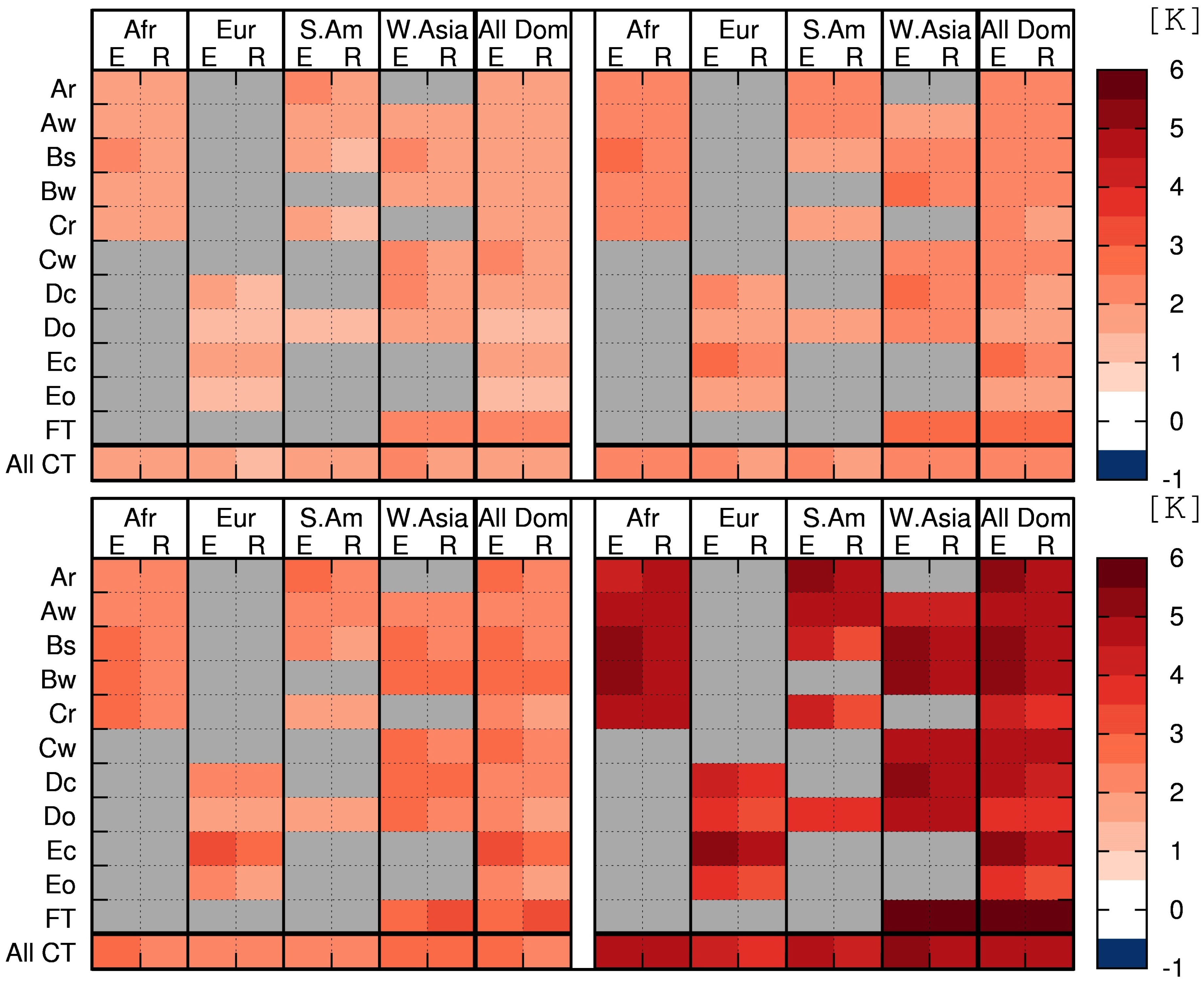
4.2. Global and Regional Climate Change Signals

The climate change signal in mean temperature and precipitation as defined in Section 3, is investigated in this section for MPI-ESM and REMO. A potential dependence of the climate change signal on climate zone (based on CRU and independent of the actual model region) is investigated.
We analyzed to what extent the spatial variance of the signal difference between GCM and RCM can be attributed to the specific climatic conditions within a certain climate type, following an analysis of variance (ANOVA) approach. As result, we found that the Köppen-Trewartha climate types explain 10.3% of the variance for temperature and 23.7% for precipitation. The value for temperature is quite low and might not be significant. For precipitation a considerable part of the signal difference can be attributed to climate types. In the following, we do the signal evaluations consequently for climate types and continents according to the evaluations of the historical climate.

4.2.1. Temperature

Figure 3 shows the climate change signal for temperature for the period 2071–2100 in comparison to the reference period 1971–2000 for the RCP 4.5 scenario in the upper row and for the RCP 8.5 scenario in the bottom row. In the left column the results of MPI-ESM are shown. The right part of Figure 3 shows dynamically downscaled results with REMO for the different CORDEX domains. The investigated model domains are included in all plots for better orientation.
Overall, the climate change signal simulated by both models for both scenarios is always greater than 1 K. The temperature change signal exceeds 5 K for major regions in both models for the RCP 8.5 scenario. In general, Figure 3 shows a similar pattern in the distribution of the climate change signal for temperature. By dynamical downscaling of the MPI-ESM data with REMO, the horizontal distribution of the climate change signal for temperature gains in heterogeneity. In the REMO, most of the hot spot regions of the MPI-ESM, e.g., the Amazon Basin area of South-America, are horizontally less extended, which can be observed in both scenarios. In summary for the horizontal patterns, the temperature change signal is maintained after dynamically downscaling the MPI-ESM simulations with REMO.
A regional specific analysis is done for the Köppen-Trewartha classes for each CORDEX domain. In Figure 4 the climate change signal of temperature is analyzed for the Köppen-Trewartha climate types, following their horizontal distribution as shown in Figure 1.
The analysis is done for the two time slices 2036–2065 and 2071–2100, shown on the left-hand side and on the right-hand side of Figure 4, respectively. Matrices for scenarios RCP 4.5 and and RCP 8.5 are shown at the top and at the bottom of Figure 4, respectively. All regions are analyzed for the MPI-ESM (marked with E) and REMO (marked with an R).
All four matrices of Figure 4 show that the majority of the climate change signals for temperature downscaled with REMO are lower or at least on the same level as the MPI-ESM results. This feature remains robust, even if the REMO simulation is compared to the other two MPI-ESM realizations (not shown). There are two exceptions in the simulations under RCP 8.5 conditions: one for the Tropical Humid (Ar) region over Africa, where REMO simulates higher temperature for the period 2071–2100, which can also be seen in the horizontal plots (see Figure 3, lower right); the other exception is in the period 2036–2065, for the West Asian Köppen-Trewartha class FT (Tundra/Highland). For both exceptions, the temperature change signal downscaled by REMO is higher than the signal of the MPI-ESM simulation for that area. In the case of the FT region of West Asia the higher REMO yearly mean temperature change signal for the RCP 4.5 of the period 2036–2065 is only a little higher, but directly at the lower edge of the 3.5 to 4 K class of the temperature change signal.
Figure 3. MPI-ESM (LR) and REMO climate change signals for annual mean temperature. The climate change signal for temperature is plotted in K as simulated by the Earth system model MPI-ESM (LR) (left panels) and the regional climate model REMO (right panels). In the upper panels the climate change signal for RCP 4.5 is shown, while the lower panels show the climate change signals for RCP 8.5. The future time period 2071–2100 is compared to the reference time period 1971–2000.
Atmosphere 04 00214 g003
The RCP 4.5 (2036–2065) for different Köppen-Trewartha classes reveals, for MPI-ESM and REMO simulations a temperature increase of at least 0.5 K in comparison to the reference period. The maximal difference for all fields of RCP 4.5 (2036–2065) is about 2 K for MPI-ESM and REMO. Within RCP 4.5 (2071–2100) a similar variability in all Köppen-Trewartha classes can be observed. Almost all fields show a temperature change signal, which is stronger than 1 K. Nevertheless, the maximal temperature difference within all fields of the matrix for RCP 4.5 (2071–2100) is still lower than 3 K, for the downscaled data even lower than 2 K.
Figure 4. Climate change signals for each domain and each climate type for annual mean temperature. The climate change signals are depicted for temperature for RCP 4.5 (upper plot) and for RCP 8.5 (lower plot) considering only gridboxes for one specific climate type per region. Climate change signals as simulated by MPI-ESM (LR) (E) and REMO (R) are plotted on the left-hand side and on the ride-hand-side, respectively. The time periods considered are 2036–2065 (left panel) and 2071–2100 (right panel) compared to the time period 1971–2000. Climate types that are not present in the respective domain are depicted in gray.
Atmosphere 04 00214 g004
Comparing the time slices and RCP scenarios with each other, the range of the temperature climate change signal is similar between RCP 8.5 (2036–2065) and RCP 4.5 (2071–2100). In RCP 8.5 (2036–2065) the mean temperature increase is about 2.5 K, and therefore by 0.5 K higher than in RCP 4.5 (2071–2100). Differences between Köppen-Trewartha classes in RCP 8.5 (2071–2100) are higher in comparison to RCP 4.5 (2071–2100) and vary from 1 to 3.5 K.
Altogether, the strongest temperature change signal is simulated for the RCP 8.5 scenario in the period 2071–2100. Here the minimal temperature change signal for all Köppen-Trewartha classes is greater than 3 K, with the maximal temperature change signal being even greater than 6 K in the Himalayan Highlands. The variation within the Köppen-Trewartha classes is greater than 3 K.
In the Africa Europe overlapping region, the differences of the climate change signals are rather small for RCP 8.5 at the end of the century (2071–2100). They range mainly up to 0.4 K, while the climate change signal itself lies between 3 K and 4 K in this region. The overlapping region of Africa and West Asia shows a similar behavior-climate change signal mainly liying between 3 K and 4 K, while the differences of signals as simulated in the African domain and in the West Asian domain are mainly below 0.4 K. For the other RCPs and for the middle of the century time slice (2036–2065), differences are smaller, except for the case of RCP 2.6 over the Africa/West Asia overlapping region, where the differences are up to 1 K over the Arabian Peninsula (not shown).

4.2.2. Precipitation
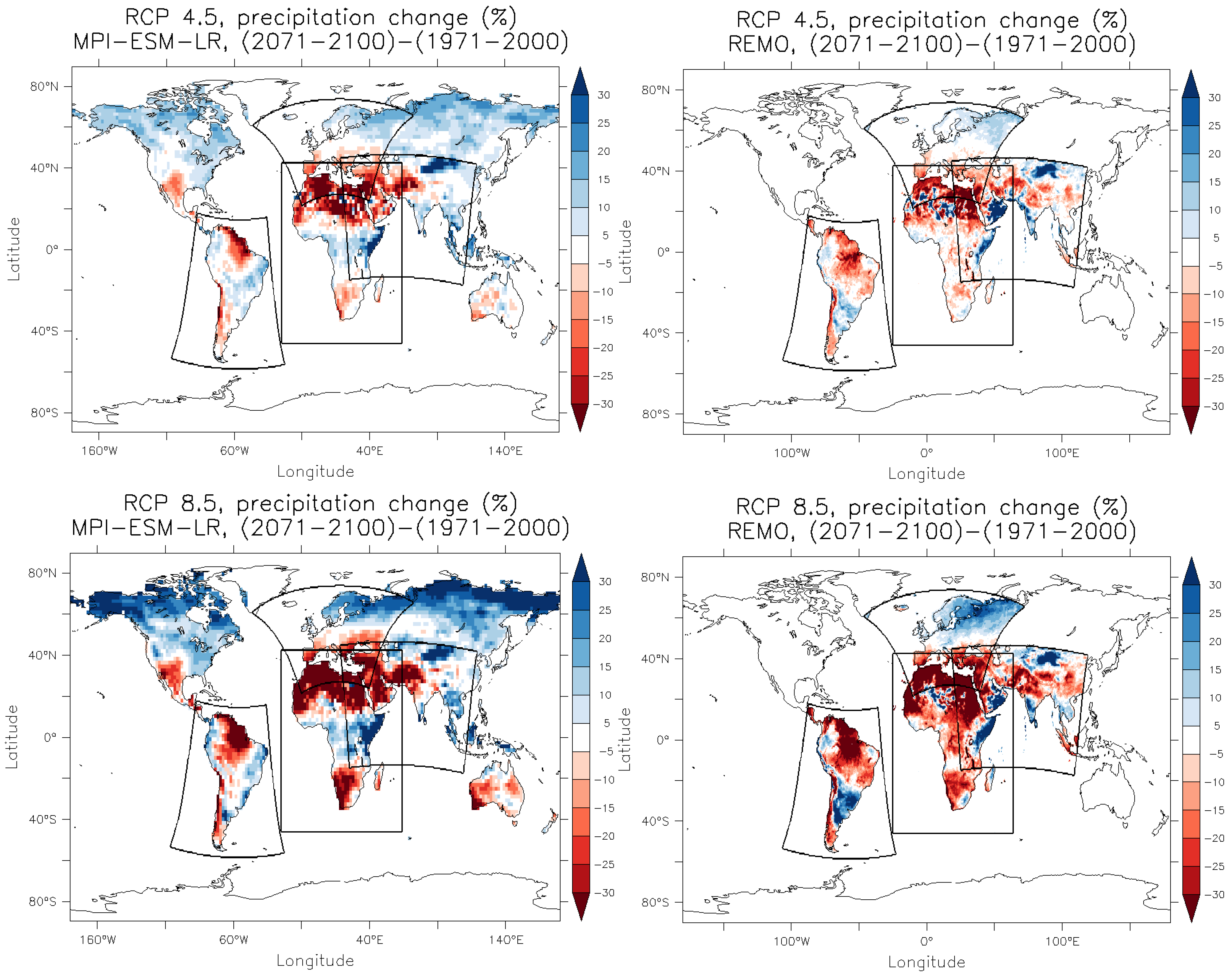
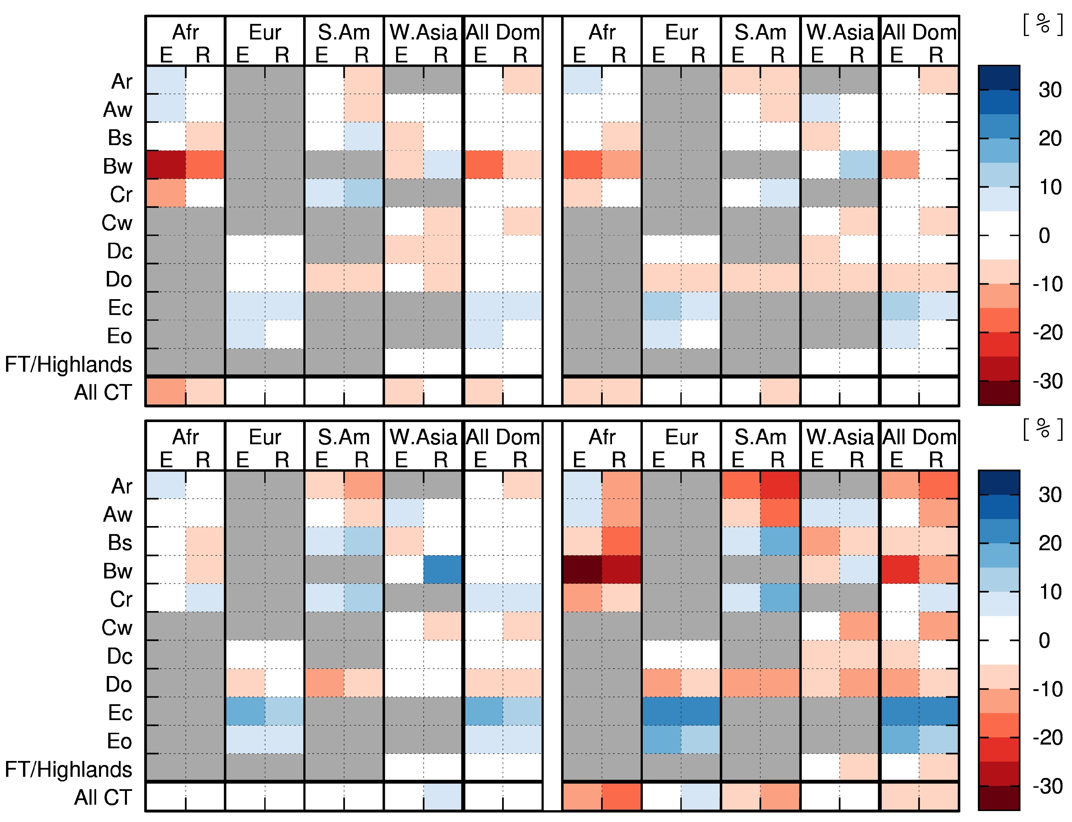
As precipitation is more variable in space and time than temperature, due to the large inter-annual variability of the rainfall amounts, small systematic changes are more difficult to detect. In Figure 5, we show the climate change signal for precipitation for the period 2071–2100 in comparison to the reference period 1971–2000 as a relative difference. The effect of climate change on precipitation is represented more intuitively by a relative measure, even though this might lead to difficulties in low precipitation areas.
In the top row of Figure 5, the results for the RCP 4.5 scenario are presented. The results for the RCP 8.5 are shown in the bottom row. The left column represents the results of the MPI-ESM, and the right column shows the dynamically downscaled results.
In both RCP scenarios and for both models, a decrease in precipitation of more than 30% is seen for the northeastern coast of South America, as well as for the western coast of North Africa. For the African area of the Sahara, the high relative precipitation differences are due to extremely low precipitation rates. Therefore the arid zones (compare Dry Arid (BW) and Dry Semi-Arid (BS) of Figure 1) cannot be easily interpreted for relative precipitation changes (Figure 6). In the Congo region in Central Africa, where the tropical climate types Ar and Aw dominate, also the precipitation change signal is modified by the regional model in RCP 4.5 and RCP 8.5 to drier conditions. Whereas the global model projects a precipitation increase (which is consistent among all three MPI-ESM realizations (not shown)), the regional model simulates a decrease in precipitation. In RCP 8.5 to the end of the 21st century this effect is most pronounced. Additionally for Africa, the area of the climate type Subtropical Humid (Cr), should be interpreted with care, as this class is mistakenly assigned to some grid boxes over the Sahara region on the basis of CRU data. Please note that for the matrix-plots these areas are not excluded for the precipitation analysis but cannot be discussed.
Within Figure 5 the results of the downscaled REMO show a very detailed pattern compared to MPI-ESM. For example in South America under RCP 4.5 condition, the pattern of the decreased precipitation change follows the course of the Amazon River instead of concentrating on the coastal border. On the other hand, the pattern of the change in dynamically downscaled precipitation in the Amazon Basin is widely extended to the south for both RCP scenarios. Here, the climate change signal for precipitation changes from an increase in MPI-ESM to a decrease in REMO. For the South American continent, the areas of tropical humid (Ar) and tropical wet-dry (Aw) conditions for the MPI-ESM contain regions of precipitation increase as well as precipitation decrease. Therefore the area averaged values are close to zero.
Figure 5. MPI-ESM (LR) and REMO climate change signals for annual precipitation sums. The climate change signal for precipitation is plotted in mm/day as simulated by the Earth system model MPI-ESM (LR) (left panels) and the regional climate model REMO (right panels). In the upper panels the climate change signal for RCP 4.5 is shown, while the lower panels show the climate change signals for RCP 8.5. The future time period 2071–2100 is compared to the reference time period 1971–2000.
Atmosphere 04 00214 g005
Differences between the climate change signals of precipitation in the overlapping region of Africa and Europe lie mainly below 10 percentage points with a climate change signal of more than 30 percent for RCP 8.5 at the end of the century (2071–2100). In the overlapping region of Africa and West Asia, differences are typically less than 15 percentage points, with the exception of the coastal areas of the Horn of Africa and the Arabian Peninsula, where differences lie well above 20 percentage points, with climate change signals of more than 30 percent. For the other RCPs and for the middle of the century time slice (2036–2065), the magnitudes of the differences are mainly similar or smaller (not shown).
Figure 6. Climate change signals for each domain and each climate type for annual precipitation sums. The climate change signals are depicted for precipitation for RCP 4.5 (upper plot) and for RCP 8.5 (lower plot), considering only grid boxes for one specific climate type per region. Climate change signals as simulated by MPI-ESM (LR) (E) and REMO (R) are plotted on the left-hand side and on the ride-hand-side, respectively. The time periods considered are 2036–2065 (left panel) and 2071–2100 (right panel), compared to the time period 1971–2000. Climate types that are not present in the respective domain are depicted in gray.
Atmosphere 04 00214 g006

4.2.3. Discussion

Some differences between the climate change signals simulated by the regional and the global model shown in Figure 3 and Figure 5 are restricted to a certain region, as in the case of central Africa. This is the only region, located mainly within the Ar climate type, where the temperature increase is larger in the RCM simulation for the RCP 8.5 at the end of the 21st century. A positive feedback on temperature due to different non-linear processes in the regional model might occur at a certain level of warming.
The global and regional model processes leading to the opposite precipitation signals of the regional and the global simulations in the projected climate over central Africa are presently investigated by Saeed et al. [68]. They show that more frequent heavy precipitation events occur in REMO and lead to higher surface runoff than in the GCM. The higher runoff causes less infiltration into the soil and, thus, reduces soil moisture content. Therefore, evaporation is reduced and temperature increases. The reduced local water recycling leads to less mean precipitation and stronger warming in this region.
Some modifications of the climate change signal projected by the RCM compared to the GCM occur in certain climate types, independent of which continent they are located on. In these cases, special regional and local characteristics of the climate types seem to contribute to the modifications. Such as within all arid climate types (BW and BS), and within the temperate continental climate type (Dc), REMO simulates a smaller warming signal than the driving MPI-ESM in all domains. This common feature becomes more pronounced in the RCP 8.5 at the end of the 21st century. Systematic differences also occur in the tropical climate types Ar and Aw, where REMO modifies the precipitation signal simulated by the GCM not only in Central Africa but also in Ar and Aw in South America and also in Indonesia (see Figure 5) to drier climate conditions. In all cases, this common feature is negligible in the RCP 2.6 (not shown), slightly present in the RCP 4.5 and becomes most prominent in the RCP 8.5 at the end of the 21st century. A common feature can also be seen in the oceanic temperate climate type Do, where both MPI-ESM and REMO simulate precipitation decreases RCP 4.5 and RCP 8.5 at the end of the century. The subarctic continental climate type Ec is only present in Europe, here both models project precipitation increases in both scenarios with higher values in 2071–2100. Several differences between GCM and RCM appear only or more pronounced at a certain level of warming as in the RCP 8.5 at the end of the 21st century, which might be caused by different non-linear processes at different spatial scales in the regional and global model.
The difference in the climate change signal of temperature in the overlapping regions is in general rather small compared to the climate change signal itself. This indicates that the choice of the model domain is of minor importance in this case. Also, different biases in the control period do not influence the annual mean climate change signal significantly, as can be seen in the case of the Africa/West Asia overlapping region, where we saw a larger bias in the West Asia control run compared to observations than in the African domain.
In the case of precipitation, the differences in the climate change signals are smaller in the case of the Africa/Europe overlapping domain, probably due to a more similar circulation pattern in both domains due to the similar location of the Western boundary (refer to Section 4.1.3). The differences in the areas of the Horn of Africa and the Arabian peninsula could be related to differences in the simulated circulation patterns over the Indian Ocean (refer to Section 4.1.3). As these regions are very arid, absolute differences are relatively small.

5. Conclusions

In this study we investigate how the simulated historical climate and the climate change projections of the GCM MPI-ESM are modified by dynamic downscaling with the RCM REMO. The global simulations have been downscaled with REMO over the four CORDEX domains South America, Europe, Africa and West Asia using a similar model setup. We compare features of the simulated global and regional climate under different anthropogenic forcing within continents and climate types. The analysis is done on the basis of annual mean climate parameters to get a general overview of major modifications in mean climate. From this, further studies will follow to investigate important features at higher temporal resolution and with more detailed spatial patterns.
The representation of the historical time period in both the global and regional simulations is evaluated in comparison to CRU observational data. In general, the historical climate is well represented by both models, but some different biases in the global and the regional simulations can be seen. In South America, the global simulation results show a warm bias over the Amazon Basin, which disappears in large parts of this region in the RCM simulations. A predecessor REMO version showed a similar warm bias which was substantially reduced by a better representation of tropical forest rooting depths [28]. The strong influence of the lower boundary points to the importance of an appropriate representation of vegetation and soil properties within climate models. Especially in regions with strong land-atmosphere coupling like in the Amazon basin, realistic land surface representations at high spatial resolution have the potential to improve the global simulations by regional downscaling. Furthermore, the climate change signal is modified in the Amazon Basin with less temperature increase simulated by the RCM in some parts of this region. The regional simulation shows a cold bias over northern Africa, while in the global results a slight warm bias in some parts of this area occur. A systematic cold bias occurs in large parts of the West Asian domain in the regional simulations, whereas the global simulation results show a distinct warm bias. However, with respect to the simulated climate change signals, the projected temperature increase is similar over West Asia in the regional and global simulations, indicating that the cold bias in the historical simulation does not affect the annual mean climate change signal in this region.
The bias in the control period has no apparent influence on the climate change signal under the conditions of this study, as can be seen from the regions where the domains overlap. Especially in the overlapping region of Africa and West Asia, where the bias versus observed temperatures differ significantly for the two domains, the climate change signal for temperature is similar.
In general, similar mean temperature change signals are projected by the RCM in comparison to the GCM. In several regions and in certain climate types as the arid climate types (BW and BS) and the temperate continental climate type (Dc) the temperature increase is somewhat lower in the RCM projections. One exception is the Congo region in Central Africa, where the temperature increase is greater in the RCM simulation for RCP 8.5 at the end of the century.
The precipitation change signals are spatially heterogeneous with some different patterns in the RCM and GCM simulations. A common feature can be seen in the oceanic temperate climate type Do, where both MPI-ESM and REMO simulate precipitation decreases under RCP 4.5 and RCP 8.5, at the end of the century. A systematic modification of the precipitation signal simulated by the GCM occurs in the tropical climate types Ar and Aw in all model domains. Here, the regional model simulates drier climate conditions. This feature gets more pronounced with strong radiative forcing in the RCP 8.5 at the end of the 21st century. In central Africa, the precipitation signal even differs in sign in RCP 8.5 in 2071–2100, with precipitation increases in MPI-ESM and decreases in REMO. At the same time, temperature increase is stronger in the regional simulations. The study of Saeed et al. [68] refers the drier and warmer climate conditions projected by the regional model in central Africa to much more frequent heavy precipitation events and thus stronger surface runoff and less infiltration of water into the soil, leading to reduced local water recycling and less evaporative cooling in this region. If similar processes occur within the tropical climate types in South America and Indonesia, it will be investigated in following studies. A further interesting research question is if other regional climate models modify the global MPI-ESM simulations in a similar way. In this study, we defined the climate type regions according to CRU data in order to fix the evaluation regions for comparison. They might not completely overlap with the GCM and RCM data of the historical simulations and also be shifted in the climate change simulations. In a further study, it would be interesting to analyze the spatial shift of climate zones in the climate projections.
This study can help to interpret global and regional climate change signals simulated by the model chain MPI-ESM/REMO. As it is only one GCM-RCM model combination, it cannot provide a complete assessment of the climate change signals in the different regions. For this, an ensemble of model simulations has to be used. As different models lead to different projections, all available global/regional model combinations need to be applied in order to achieve the best approximation of possible climate change signals. This analysis can be done in future studies, when a sufficiently large ensemble of simulations on the basis of the different RCPs becomes available, e.g., within the frame of CMIP5/CORDEX.

Acknowledgments

REMO simulations for South America and West Asia were conducted under various projects such as, CLARIS-LPB (FP7 Grant Agreement No. 212492) and HighNoon (FP7 Grant Agreement No. 227087), respectively. The REMO simulations for the European and African domain were performed under the “Konsortial" share at the German Climate Computing Center (DKRZ), for which we are further thankful for the support. We thank the anonymous reviewers for their constructive and useful suggestions.

Conflict of Interest

The authors declare no conflict of interest.

References

  1. Intergovernmental Panel on Climate Change (IPCC). Climate Change 2007: The Physical Science Basis. Contribution of Working Group I to the Fourth Assessment Report of the Intergovernmental Panel on Climate Change; Cambridge University Press: Cambridge, UK/New York, NY, USA, 2007; p. 996. [Google Scholar]
  2. Chen, H.; Sun, J.; Chen, X.; Zhou, W. CGCM projections of heavy rainfall events in China. Int. J. Climatol. 2012, 32, 441–50. [Google Scholar] [CrossRef]
  3. Choi, K.S.; Cha, Y.M. Change in future tropical cyclone activity over the western North Pacific under global warming scenario. Nat. Hazards 2012, 64, 1125–1140. [Google Scholar] [CrossRef]
  4. Brown, J.; Moise, A.; Delage, F. Changes in the South Pacific convergence zone in IPCC AR4 future climate projections. Clim. Dyn. 2012, 39, 1–19. [Google Scholar] [CrossRef]
  5. Brown, J.; Power, S.; Delage, F.; Colman, R.; Moise, A. Evaluation of the South Pacific Convergence Zone in IPCC AR4 climate model simulations of the twentieth century. J. Clim. 2011, 24, 1565–1582. [Google Scholar] [CrossRef]
  6. McAfee, S.; Russell, J.; Goodman, P. Evaluating IPCC AR4 cool-season precipitation simulations and projections for impacts assessment over North America. Clim. Dyn. 2011, 37, 2271–2287. [Google Scholar] [CrossRef]
  7. Ashfaq, M.; Shi, Y.; wen Tung, W.; Trapp, R.; Gao, X. Suppression of south Asian summer monsoon precipitation in the 21st century. Geophys. Res. Lett. 2009, 36, L01704. [Google Scholar] [CrossRef]
  8. Haensler, A.; Hagemann, S.; Jacob, D. The role of the simulation setup in a long-term high-resolution climate change projection for the southern African region. Theor. Appl. Climatol. 2011, 106, 153–169. [Google Scholar] [CrossRef]
  9. Karmalkar, A.; Bradley, R.; Diaz, H. Climate change in Central America and Mexico: Regional climate model validation and climate change projections. Clim. Dyn. 2011, 37, 605–629. [Google Scholar] [CrossRef]
  10. Karmalkar, A.V.; Bradley, R.S.; Diaz, H.F. Climate change scenario for Costa Rican montane forests. Geophys. Res. Lett. 2008, 35, L11702. [Google Scholar] [CrossRef]
  11. MacKellar, N.C.; Hewitson, B.C.; Tadross, M.A. Namaqualand’s climate: Recent historical changes and future scenarios. J. Arid Environ. 2007, 70, 604–614. [Google Scholar] [CrossRef]
  12. Chou, S.; Marengo, J.; Lyra, A.; Sueiro, G.; Pesquero, J.; Alves, L.; Kay, G.; Betts, R.; Chagas, D.; Gomes, J.; Bustamante, J.; Tavares, P. Downscaling of South America present climate driven by 4-member HadCM3 runs. Clim. Dyn. 2012, 38, 635–653. [Google Scholar] [CrossRef]
  13. Marengo, J.; Chou, S.; Kay, G.; Alves, L.; Pesquero, J.; Soares, W.; Santos, D.; Lyra, A.; Sueiro, G.; Betts, R.; et al. Development of regional future climate change scenarios in South America using the Eta CPTEC/HadCM3 climate change projections: Climatology and regional analyses for the Amazon, São Francisco and the Paraná River basins. Clim. Dyn. 2012, 38, 1829–1848. [Google Scholar] [CrossRef]
  14. Vigaud, N.; Roucou, P.; Fontaine, B.; Sijikumar, S.; Tyteca, S. WRF/ARPEGE-CLIMAT simulated climate trends over West Africa. Clim. Dyn. 2011, 36, 925–944. [Google Scholar] [CrossRef]
  15. Jacob, D.; Bärring, L.; Christensen, O.B.; Christensen, J.H.; de Castro, M.; Déqué, M.; Giorgi, F.; Hagemann, S.; Hirschi, M.; Jones, R.; et al. An inter-comparison of regional climate models for Europe: Model performance in present-day climate. Clim. Chang. 2007, 81, 31–52. [Google Scholar] [CrossRef]
  16. Inatsu, M.; Kimoto, M. A scale interaction study on east asian cyclogenesis using a general circulation model coupled with an interactively nested regional model. Mon. Wea. Rev. 2009, 137, 2851–2868. [Google Scholar] [CrossRef]
  17. Gomez, E.S.; Somot, S.; Deque, M. Ability of an ensemble of regional climate models to reproduce weather regimes over Europe-Atlantic during the period 1961–2000. Clim. Dyn. 2009, 33, 723–736. [Google Scholar] [CrossRef]
  18. Mariotti, L.; Coppola, E.; Sylla, M.B.; Giorgi, F.; Piani, C. Regional climate model simulation of projected 21st century climate change over an all-Africa domain: Comparison analysis of nested and driving model results. J. Geophys. Res. 2011, 116, D15111. [Google Scholar] [CrossRef]
  19. Christensen, J.H.; Carter, T.R.; Giorgi, F. PRUDENCE employs new methods to assess European climate change. Eos. Trans. AGU 2002, 83, 147–147. [Google Scholar] [CrossRef]
  20. Hewitt, C.D. Ensembles-based predictions of climate changes and their impacts. Eos. Trans. AGU 2004, 85, 566–566. [Google Scholar] [CrossRef]
  21. Giorgi, F.; Diffenbaugh, N.S.; Gao, X.J.; Coppola, E.; Dash, S.K.; Frumento, O.; Rauscher, S.A.; Remedio, A.R.; Sanda, I.S.; Steiner, A.; et al. The regional climate change hyper-matrix framework. Eos. Trans. AGU 2008, 89, 445–446. [Google Scholar] [CrossRef]
  22. Giorgi, F.; Jones, C.; Asrar, G. Addressing climate information needs at the regional level: The CORDEX framework. WMO Bull. 2009, 58, 175–183. [Google Scholar]
  23. Trewartha, G. An Introduction to Climate, 3rd ed.; McGraw-Hill: New York, NY, USA, 1954. [Google Scholar]
  24. Nikulin, G.; Jones, C.; Giorgi, F.; Asrar, G.; Buechner, M. Precipitation climatology in an ensemble of CORDEX-Africa regional climate simulations. J. Clim. 2012, 25, 6057–6078. [Google Scholar] [CrossRef]
  25. Giorgi, F.; Coppola, E.; Solmon, F.; Mariotti, L.; Sylla, M.B. RegCM4: Model description and preliminary tests over multiple CORDEX domains. Clim. Res. 2012, 52, 7–29. [Google Scholar] [CrossRef]
  26. Ozturk, T.; Altinsoy, H.; Turkes, M.; Kurnaz, M.L. Simulation of temperature and precipitation climatology for the Central Asia CORDEX domain using RegCM 4.0. Clim. Res. 2012, 52, 63–76. [Google Scholar] [CrossRef]
  27. Diro, G.T.; Rauscher, S.A.; Giorgi, F.; Tompkins, A.M. Sensitivity of seasonal climate and diurnal precipitation over Central America to land and sea surface schemes in RegCM4. Clim. Res. 2012, 52, 31–48. [Google Scholar] [CrossRef]
  28. Jacob, D.; Elizalde, A.; Haensler, A.; Hagemann, S.; Kumar, P.; Podzun, R.; Rechid, D.; Remedio, A.R.; Saeed, F.; Sieck, K.; et al. Assessing the transferability of the regional climate model REMO to different coordinated regional climate downscaling experiment (CORDEX) regions. Atmosphere 2012, 3, 181–199. [Google Scholar] [CrossRef]
  29. Taylor, K.E.; Stouffer, R.J.; Meehl, G.A. An overview of CMIP5 and the experiment design. Bull. Amer. Meteor. Soc. 2012, 93, 485–498. [Google Scholar] [CrossRef]
  30. Moss, R.H.; Edmonds, J.A.; Hibbard, K.A.; Manning, M.R.; Rose, S.K.; van Vuuren, D.P.; Carter, T.R.; Emori, S.; Kainuma, M.; Kram, T.; et al. The next generation of scenarios for climate change research and assessment. Nature 2010, 463, 747–756. [Google Scholar] [CrossRef] [PubMed]
  31. Jacob, D.; Podzun, R. Sensitivity studies with the regional climate model REMO. Meteorol. Atmos. Phys. 1997, 63, 119–129. [Google Scholar] [CrossRef]
  32. Jacob, D. A note to the simulation of the annual and inter-annual variability of the water budget over the Baltic Sea drainage basin. Meteorol. Atmos. Phys. 2001, 77, 61–73. [Google Scholar] [CrossRef]
  33. Stevens, B.; Giorgetta, M.; Esch, M.; Mauritsen, T.; Crueger, T.; Rast, S.; Salzmann, M.; Schmidt, H.; Bader, J.; Block, K.; et al. The atmospheric component of the MPI-M earth system model: ECHAM6. J. Adv. Model. Earth Syst. 2013. in review. [Google Scholar] [CrossRef]
  34. Jungclaus, J.H.; Fischer, N.; Haak, H.; Lohmann, K.; Marotzke, J.; Matei, D.; Mikolajewicz, U.; Notz, D.; von Storch, J.S. Characteristics of the ocean simulations in MPIOM, the ocean component of the MPI Earth System Model. J. Adv. Model. Earth Syst. 2013. in review. [Google Scholar] [CrossRef]
  35. Six, K.D.; Maier-Reimer, E. What controls the oceanic dimethylsulfide (DMS) cycle? A modeling approach. Glob. Biogeochem. Cy. 2006, 20, GB4011. [Google Scholar]
  36. Ilyina, T.; Six, K.D.; Segschneider, J.; Maier-Reimer, E.; Li, H.; Núñez-Riboni, I. The global ocean biogeochemistry model HAMOCC: Model architecture and performance as component of the MPI-earth system model in different CMIP5 experimental realizations. J. Adv. Model. Earth Syst. 2013, in press. [Google Scholar] [CrossRef]
  37. Reick, C.H.; Raddatz, T.; Brovkin, V.; Gayler, V. The representation of natural and anthropogenic land cover change in MPI-ESM. J. Adv. Model. Earth Syst. 2013, in press. [Google Scholar] [CrossRef]
  38. Brovkin, V.; Boysen, L.; Raddatz, T.; Gayler, V.; Loew, A.; Claussen, M. Evaluation of vegetation cover and land-surface albedo in MPI-ESM CMIP5 simulations. J. Adv. Model. Earth Syst. 2013, 5, 1–10. [Google Scholar] [CrossRef]
  39. Giorgetta, M.A.; Jungclaus, J.H.; Reick, C.H.; Legutke, S.; Brovkin, V.; Crueger, T.; Esch, M.; Fieg, K.; Glushak, K.; Gayler, V.; et al. Climate change from 1850 to 2100 in MPI-ESM simulations for the coupled model intercomparison Project 5. J. Adv. Model. Earth Syst. 2013. in review. [Google Scholar]
  40. Roeckner, E.; Bäuml, G.; Bonaventura, L.; Brokopf, R.; Esch, M.; Giorgetta, M.; Hagemann, S.; Kirchner, I.; Kornblueh, L.; Manzini, E.; et al. The Atmospheric General Circulation Model ECHAM-5: Part I. Model Description; Technical Report 349; Max-Planck-Institute for Meteorology: Hamburg, Germany, 2003. [Google Scholar]
  41. Jungclaus, J.H.; Keenlyside, N.; Botzet, M.; Haak, H.; Luo, J.J.; Latif, M.; Marotzke, J.; Mikolajewicz, U.; Roeckner, E. Ocean circulation and tropical variability in the coupled model ECHAM5/MPI-OM. J. Clim. 2006, 19, 3952–3972. [Google Scholar] [CrossRef]
  42. Hurtt, G.; Chini, L.; Frolking, S.; Betts, R.; Feddema, J.; Fischer, G.; Fisk, J.; Hibbard, K.; Houghton, R.; Janetos, A.; et al. Harmonization of land-use scenarios for the period 1500–2100: 600 years of global gridded annual land-use transitions, wood harvest, and resulting secondary lands. Clim. Chang. 2011, 109, 117–161. [Google Scholar] [CrossRef]
  43. Moss, R.; Babiker, M.; Brinkman, S.; Calvo, E.; Carter, T.; Edmonds, J.; Elgizouli, I.; Emori, S.; Erda, L.; Hibbard, K.A. Towards New Scenarios for Analysis of Emissions, Climate Change, Impacts, and Response Strategies; Technical Report PNNL-SA-63186; Intergovernmental Panel on Climate Change: Geneva, Switzerland, 2008. [Google Scholar]
  44. Vuuren, D.P.; Stehfest, E.; Elzen, M.; Kram, T.; Vliet, J.; Deetman, S.; Isaac, M.; Klein Goldewijk, K.; Hof, A.; Mendoza Beltran, A.; Mendoza Beltran, A.; et al. RCP2.6: Exploring the possibility to keep global mean temperature increase below 2°C. Clim. Chang. 2011, 109, 95–116. [Google Scholar] [CrossRef]
  45. Thomson, A.M.; Calvin, K.V.; Smith, S.J.; Kyle, P.; Volke, A.; Patel, P.; Delgado-Arias, S.; Bond-Lamberty, B.; Wise, M.A.; Clarke, L.E.; et al. RCP4.5: A pathway for stabilization of radiative forcing by 2100. Clim. Chang. 2011, 109, 77–94. [Google Scholar] [CrossRef]
  46. Riahi, K.; Rao, S.; Krey, V.; Cho, C.; Chirkov, V.; Fischer, G.; Kindermann, G.; Nakicenovic, N.; Rafaj, P. RCP 8.5—A scenario of comparatively high greenhouse gas emissions. Clim. Chang. 2011, 109, 33–57. [Google Scholar] [CrossRef]
  47. Majewski, D. The Europa-Modell of the Deutscher Wetterdienst. In Proceedings of ECMWF Seminar on Numerical Methods in Atmospheric Models, Reading, UK, 9–13 September 1991; Volume 2, pp. 147–191.
  48. Roeckner, E.; Arpe, K.; Bengtsson, L.; Christoph, M.; Claussen, M.; Dümenil, L.; Esch, M.; Giorgetta, M.; Schlese, U.; Schulzweida, U. The Atmospheric General Circulation Model ECHAM-4: Model Description and Simulation of Present-Day Climate; Technical Report 218; Max-Planck-Institute for Meteorology: Hamburg, Germany, 1996. [Google Scholar]
  49. Tiedtke, M. A comprehensive mass flux scheme for cumulus parameterization in large-scale models. Mon. Wea. Rev. 1989, 117, 1779–1800. [Google Scholar] [CrossRef]
  50. Nordeng, T.E. Extended Versions of the Convective Parametrization Scheme at ECMWF and Their Impact on the Mean and Transient Activity of the Model in the Tropics; Technical Momorandum 206; ECMWF Research Department, European Centre for Medium Range Weather Forecasts: Reading, UK, 1994. [Google Scholar]
  51. Pfeifer, S. Modeling Cold Cloud Processes with the Regional Climate Model REMO. Ph.D. Thesis, Max-Planck-Institute for Meteorology, Hamburg, Germany, 2006. [Google Scholar]
  52. Morcrette, J.; Smith, L.; Fourquart, Y. Pressure and temperature dependance of the absorption in longwave radiation parameterizations. Beitr. Phys. Atmos. 1986, 59, 455–469. [Google Scholar]
  53. Giorgetta, M.; Wild, M. The Water Vapour Continuum and Its Representation in Echam4; Technical Report 162; Max-Planck-Institute for Meteorology: Hamburg, Germany, 1995. [Google Scholar]
  54. Louis, J.F. Parametric model of vertical eddy fluxes in the atmosphere. Bound. Layer Meteorol. 1979, 17, 187–202. [Google Scholar] [CrossRef]
  55. Lohmann, U.; Roeckner, E. Design and performance of a new cloud microphysics scheme developed for the ECHAM4 general circulation model. Clim. Dyn. 1996, 12, 557–572. [Google Scholar] [CrossRef]
  56. Hagemann, S. An Improved Land Surface Parameter Dataset for Global and Regional Climate Models; Report 336; Max-Planck-Institute for Meteorology: Hamburg, Germany, 2002. [Google Scholar]
  57. Rechid, D.; Raddatz, T.; Jacob, D. Parameterization of snow-free land surface albedo as a function of vegetation phenology based on MODIS data and applied in climate modelling. Theor. Appl. Climatol. 2009, 95, 245–255. [Google Scholar] [CrossRef]
  58. Kumar, P.; Wiltshire, A.; Mathison, C.; Asharaf, S.; Ahrens, B.; Lucas-Picher, P.; Christensen, J.H.; Gobiet, A.; Saeed, F.; Hagemann, S.; et al. Downscaled climate change projections with uncertainty assessment over India using a high resolution multi-model approach. Sci. Total Environ. 2013, in press. [Google Scholar] [CrossRef] [PubMed]
  59. Davies, H.C. A lateral boundary formulation for multi-level prediction models. Q. J. R. Meteorol. Soc. 1976, 102, 405–418. [Google Scholar] [CrossRef]
  60. Tanré, D.; Geleyn, J.; Slingo, J. First Results of the Introduction of an Advanced Aerosol-Radiation Interaction in the ECMWF Low Resolution Global Model. In Aerosols and Their Climatic Effects; Gerber, H., Deepak, A., Eds.; A. Deepak Publishing: Hampton, VA, USA, 1984; pp. 133–177. [Google Scholar]
  61. Trewartha, G.; Horn, L. An Introduction to Climate; McGraw-Hill: New York, USA, 1980. [Google Scholar]
  62. Castro, M.; Gallardo, C.; Jylha, K.; Tuomenvirta, H. The use of a climate-type classification for assessing climate change effects in Europe from an ensemble of nine regional climate models. Clim.c Chang. 2007, 81, 329–341. [Google Scholar] [CrossRef]
  63. British Atmospheric Data Centre. CRU Datasets-CRU TS Time-Series; British Atmospheric Data Centre: Didcot, UK, 2008. [Google Scholar]
  64. Kleidon, A.; Heimann, M. Assessing the role of deep rooted vegetation in the climate system with model simulations: Mechanism, comparison to observations and implications for Amazonian deforestation. Clim. Dyn. 2000, 16, 183–199. [Google Scholar] [CrossRef]
  65. Zubler, E.M.; Lohmann, U.; Lüthi, D.; Schär, C. Intercomparison of aerosol climatologies for use in a regional climate model over Europe. Geophys. Res. Lett. 2011, 38, L15705. [Google Scholar] [CrossRef]
  66. Laprise, R.; Kornic, D.; Rapaić, M.; Šeparović, L.; Leduc, M.; Nikiema, O.; Luca, A.; Diaconescu, E.; Alexandru, A.; Lucas-Picher, P.; et al. Considerations of Domain Size and Large-Scale Driving for Nested Regional Climate Models: Impact on Internal Variability and Ability at Developing Small-Scale Details. In Climate Change; Berger, A., Mesinger, F., Sijacki, D., Eds.; Springer: Vienna, Austria, 2012; pp. 181–199. [Google Scholar]
  67. Krishnamurti, T.N.; Oosterhof, D.K.; Mehta, A.V. Air–sea interaction on the time scale of 30 to 50 days. J. Atmos. Sci 1988, 45, 1304–1322. [Google Scholar] [CrossRef]
  68. Saeed, F.; Haensler, A.; Hagemann, S.; Jacob, D. Representation of extreme precipitation events leading to opposite climate change signals over the Congo basin. Atmosphere 2013. in review. [Google Scholar] [CrossRef]

