The Copula Function-Based Probability Characteristics Analysis on Seasonal Drought & Flood Combination Events on the North China Plain

Abstract

Drought & flood events, especially the drought & flood combination events (DFCEs) on the North China Plain (NCP), known as an important grain production region in China, constitute a serious threat to China’s food security. Studies on DFCEs in this region are of great significance for the rational allocation of water resources and the formulation of integrated response strategy for droughts and floods. In this study, L-moments theory and bivariate copula method were used to evaluate the probability characteristics of seasonal DFCEs (continuous drought, continuous flood, and alternation between drought and flood) on the NCP, based on the daily precipitation data (1960–2012) at 19 meteorological stations. Results indicate the following: (1) On the NCP, the precipitation in summer accounts for 56.45%–72.02% of mean annual precipitation, and the precipitation in autumn and spring come second. The winter precipitation is the smallest (less than 4%); (2) The best-fit distribution for precipitation anomaly percentages in spring, summer and autumn are Generalized Normal (GNO), Generalized Logistic (GLO) and Pearson III (P-III) in sub-region I, respectively. While in sub-region II, they are respectively the P-III, P-III and Generalized Extreme-Value (GEV); (3) Compared with the Gumbel copula and Clayton copula, Frank copula is more suitable for spring-summer and summer-autumn precipitation anomaly percentage sequences on the NCP; (4) On the time scale, continuous drought respectively dominate in spring-summer DFCEs and in summer-autumn DFCEs on the NCP. Summer-autumn DFCEs prevail in sub-region I with the average probability value 0.34, while spring-summer DFCEs dominate in sub-region II, of which average probability value is 0.42; (5) On the spatial scale, most areas where the probability of continuous drought in spring-summer and spring drought & summer flood is relatively high are located in the northwest, northeast, and coastal parts of sub-region II; all the events with high probability of continuous drought in summer-autumn and summer flood & autumn drought occurred at the central part in the northwest of sub-region II.

1. Introduction

Due to the global warming, climate and environment have experienced significant changes, as a result of which the global average surface temperature has risen by 0.56–0.92 °C [1,2]. The increase of air temperature accelerated the rate of water cycle, thus leading to the increase in the frequency of occurrence of extreme hydrological events (i.e., droughts and floods), having brought about significant direct losses of social economy [3,4]. However, continuous droughts, continuous floods and the alternation between drought and flood between seasons become more frequent than ever along with the exacerbation of climate changes impacts [5,6], and their impacts exhibit a multi-faceted and multi-level feature. Hence, it’s essential to reinforce the studies on drought & flood combination events (DFCEs) so as to achieve the rational distribution of industry structure, the disaster risk management, and the optimized allocation of water resources.

At present, there are many studies performing characteristic analysis on drought or flood events based on copula functions. Specific to droughts, Shiau and Modarres [7] probed into the joint distribution of drought intensity, duration and frequency in Iran using the bivariate copula function. Results showed that the drought severity in humid region might be more severe under high rainfall fluctuations. Ibrahim et al. [8] have evaluated the dry conditions in Peninsular Malaysia using bivariate copula, and showed that the Galambos distribution provides the best fit for the majority of stations. Mirabbasi et al. [9] have tested several copulas to analyze the meteorological drought characteristics of the Sharafkhaneh gauge station, and come to the same conclusion as Ibrahim. According to the flood events, Zhang [10] derived bivariate distributions of flood peak and volume, and flood volume and duration through the bivariate Archimedes copula distribution, and results showed that bivariate copula distribution model fits better than others. Sraj et al. [11] have applied and compared different bivariate copulas to analyze the corresponding hydrograph volumes and durations of 58 flood events at the Litija gauging station on the Sava River in Slovenia. Results showed that the differences among most of the applied copulas were not significant. Li et al. [12] have analyzed flood peaks and flood volumes considering the historical information based on the copula.

Recently, frequency analyses of droughts or floods have been performed using multivariate copulas, which are more complex mathematically than the bivariate case [13]. Some research focused more on the drought duration, severity, and intensity to analyze the drought events by applying trivariate copulas [14,15]. And some researches devoted to the flood peak, volume, duration and suspended sediment concentration to probe into the flood events using the same kind of method as droughts [16,17,18,19]. These studies aimed at individual drought or flood events, and did not take into account the DFCEs. Meanwhile, few studies on drought, flood or DFCEs analysis using copulas have been conducted on the NCP.

This paper focuses on the probability characteristics of seasonal DFCEs on the NCP based on the L-moments theory and bivariate copula distribution, so as to provide necessary basis for the response to droughts and floods on the NCP. This paper is arranged as follows: (1) Section 2 describes the study area and data used in the study; (2) Section 3 introduces analysis methods based on the L-moments, bivariate copula distribution and goodness of fit test; (3) Section 4 provides results and discussions; (4) Finally, Section 5 draws the conclusions.

2. Study Area and Data

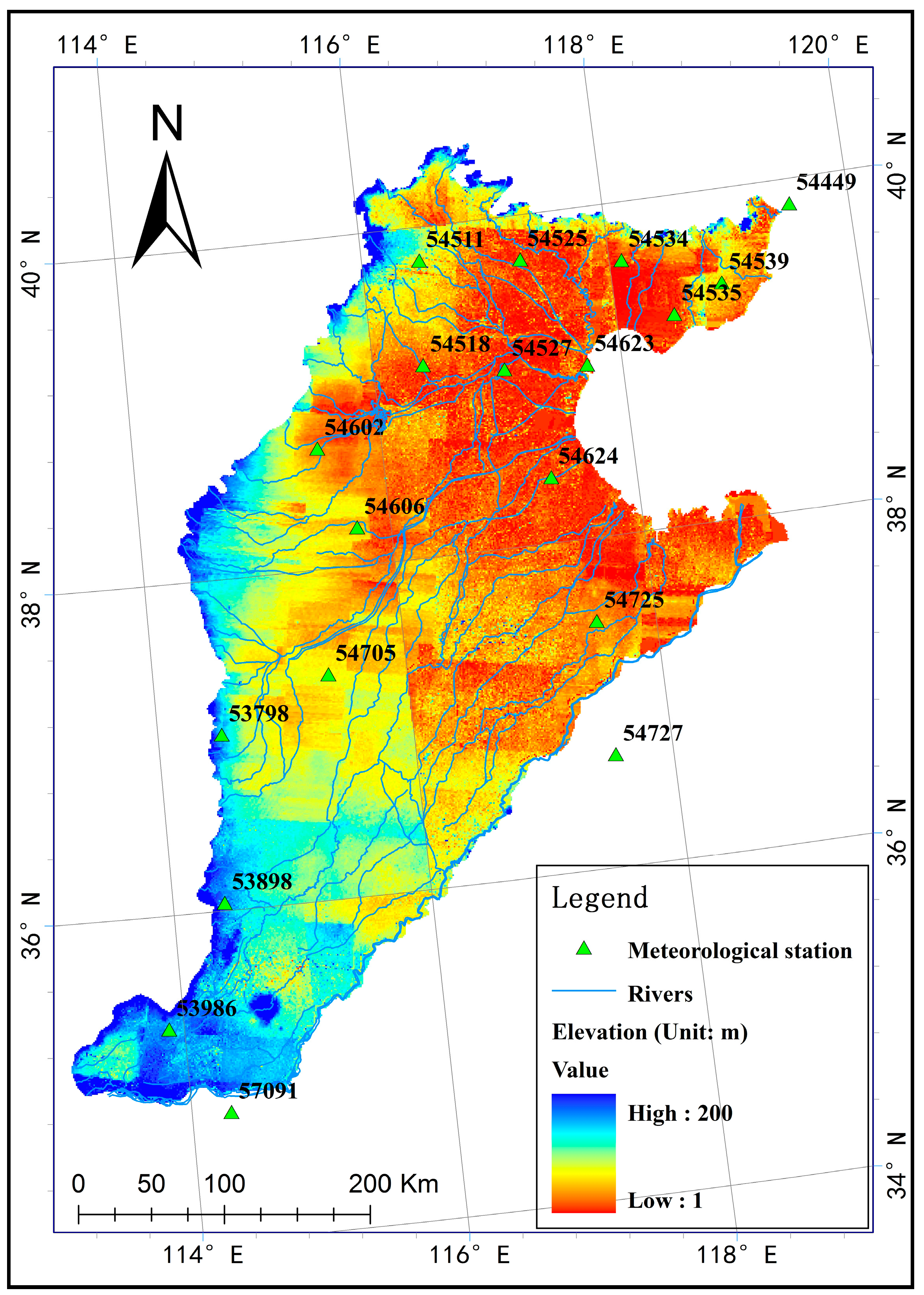
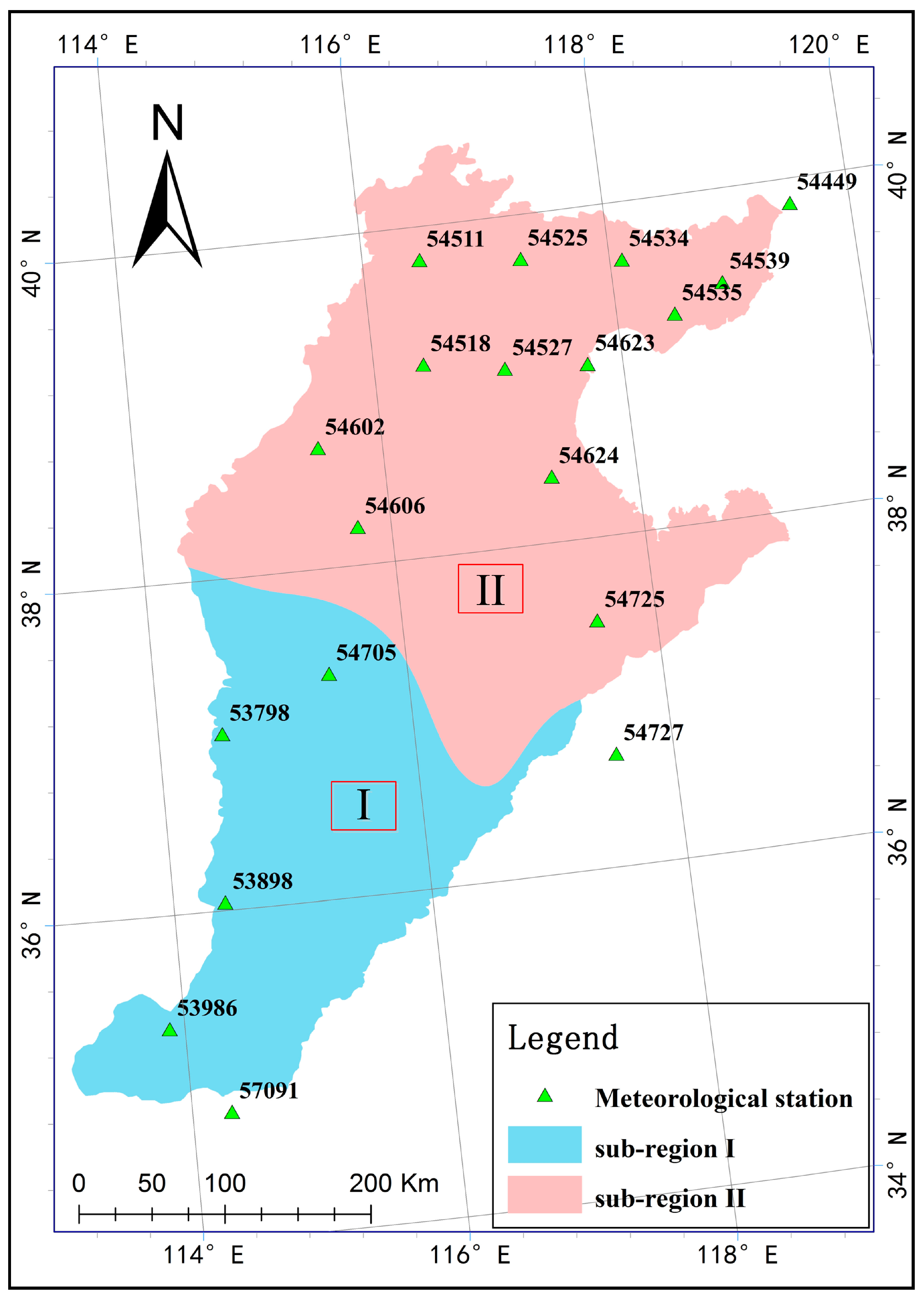
2.1. Overview of the Region of Interest

The NCP (E: 112°30′–119°30′, N: 34°46′–40°25′) is a low-lying depositional plain of the Yellow River and the Haihe River and covers an area of 136,000 km² in the east of China (Figure 1). This plain has a continental monsoon climate, where it’s dry and cold in winter, hot and rainy in summer, and dry in spring. The annual precipitation ranges from about 800 mm in the south to 500 mm in the north [20], most of which occurs from June to September. The mean annual land surface evaporation and water surface evaporation are 470 mm and 1100 mm, respectively [21]. Droughts and floods happen frequently in this region. Meanwhile, there are four clear seasons on the NCP. Spring includes March, April and May. June, July and August belong to the summer. Autumn is composed of September, October and November. And the rest months pertain to the winter. The NCP is part of the basins of the Haihe River, the Yellow River and the Luanhe River. It comprises nearly 60 rivers in different sizes, including the Tuhai River, the Majia River, and the coastal rivers in Hebei Province etc.

The NCP is substantially located in the Haihe River Basin. According to the Historical Data of Floods and Droughts at the Haihe River Basin, floods and droughts have respectively occurred 194 and 192 times at the Haihe River Basin from 1469 to 1948. During the period of 1949–1990, both floods and droughts have occurred 18 times [22]. The Haihe River Basin is also subjected to continuous occurrence of droughts and floods for years [23]. From 1470 to 1911, droughts which lasted 2 years have occurred 11 times; three consecutive years of drought has occurred 8 times. Over three consecutive years of drought has occurred 7 times, in which the longest one lasted 7 years. Moreover, there were two dry years at the Haihe River Basin from 1956 to 1998. Specific to flood, it occurred continually at the Haihe River Basin during the period of 1652–1654 and 1822–1823. Besides, the wet years lasted 12 years during the period from 1883 to 1894, including three devastating floods.

2.2. Data Sources

The daily precipitation observations (1960–2012) are collected from 19 meteorological stations (Figure 1) on the NCP. These data are derived from the National Meteorological Information Center (NMIC) [24], and has been subjected to stringent quality inspection by NMIC [25,26]. Besides, this paper makes the following provisions on data missing: Where the data for 5 days within one month is missing, the data for that month should be deemed missing. If the period of data missing reaches 1 month within a year, the data for that year should be considered missing.

Figure 1. North China Plain, meteorological stations and rivers.

Figure 1. North China Plain, meteorological stations and rivers.

3. Methodology

3.1. Theory of L-Moments

L-moments are proposed by Hosking (1990) [27] based on probability weighted moments (PWM) and represent the PWM linear combination as [28]. The most important feature of L-moments is that it is less sensitive than ordinary moments to the data sequence extremes and can obtain more robust parameter estimates. L-moments are defined as follows [29]:

Assume F(x) is the distribution function of random variable X, let X_1n ≤ X_2n ≤ … ≤ X_nn be the random sampling order statistics of X which sample size is n. The r-order linear moment of variable X should be:

$$l_r=r^{-1}{\displaystyle \sum _{i=0}^{r-1}{(-1)}^i}\left(\begin{array}{l}r-1\\ i\end{array}\right)E{X}_{r-i:r},\mathrm{ r}=\begin{array}{ccc}1,& 2,& \cdots \end{array}$$

(1)

where, EX_r-i:r means the mathematical expectation of (r-i)-order statistics when sample size is r.

The first-, second-, third-, and fourth-order sample linear moments are calculated as follows:

$$l_1=b_0; l_2=2b_1-b_0; l_3=6b_2-6b_1+b_0; l_4=20b_3-30b_2+12b_1-b_0$$

(2)

where,

$$\{\begin{array}{l}{b}_0=1/n{\displaystyle \sum _{j=1}^n{x}_{j:n}}\\ b_1=1/n{\displaystyle \sum _{j=2}^n\frac{j-1}{n-1}{x}_{j:n}}\\ b_2=1/n{\displaystyle \sum _{j=3}^n\frac{\left(j-1\right)\left(j-2\right)}{\left(n-1\right)\left(n-2\right)}{x}_{j:n}}\\ b_3=1/n{\displaystyle \sum _{j=4}^n\frac{\left(j-1\right)\left(j-2\right)\left(j-3\right)}{\left(n-1\right)\left(n-2\right)\left(n-3\right)}{x}_{j:n}}\end{array}$$

(3)

L-moments ratio is defined as follows:

$$t_2=l_2/l_1; t_3=l_3/l_2; t_4=l_4/l_2$$

(4)

where, t₂, t₃, t₄ are the L-variation coefficient (L-Cv), L-skewness coefficient (L-γ) and L-kurtosis coefficient (L-k), respectively.

3.2. Identification and Test of Homogenous Regions Based on the L-Moments

3.2.1. Identification of Homogenous Regions

The homogeneous region means the monitoring data of meteorological stations within the region could be expressed with the same probability distribution [26,29]. The identification could be performed in many ways, principally including geographical proximity principle, subjective division method, objective division method, and clustering methodology [30]. Clustering method is a multivariate statistical analysis-based standard classification method that is frequently used for hydrological partition [26]. Clustering methods mainly include partitioning methods, hierarchical methods, density-based methods, grid-based methods, model-based methods, etc. This paper employs K-means under partitioning method. However, it should be noted that, since the result of cluster analysis is not necessarily the final result, it’s necessary to make reasonable adjustments. For example, moving a meteorological station from one sub-region to another, subdividing a sub-region, merging a number of sub-regions, removing some meteorological stations, or adding new meteorological stations and performing repartition [30].

3.2.2. Screening Data Using the Discordancy Measure Test

Discordancy test is performed to check the existence of singular meteorological stations in each sub-region in the following principle:

Assume there are N meteorological stations within a certain area, and it’s possible to work out the linear moment coefficient of sample ($t_2^{\left(i\right)},t_3^{\left(i\right)},t_4^{\left(i\right)}$) for each meteorological station, i = 1, 2, …, N; let:

$$u_i={\left[t_2^{\left(i\right)},t_3^{\left(i\right)},t_4^{\left(i\right)}\right]}^T; \overline{u}=\frac{1}{N}{\displaystyle \sum _{i=1}^N{u}_i}; A={\displaystyle \sum _{i=1}^N\left(u_i-\overline{u}\right){\left(u_i-\overline{u}\right)}^T}$$

(5)

The discordancy measure D could be expressed as [29]:

$$D_i=\frac{1}{3}N{\left(u_i-\overline{u}\right)}^T{A}^{-1}\left(u_i-\overline{u}\right)$$

(6)

where, $t_2^{\left(i\right)}$ means the L-Cv of sample linear moment; $t_3^{\left(i\right)}$ represents the L-γ of sample linear moment; $t_4^{\left(i\right)}$ stands for the L-k of sample linear moment. When discordancy measure D_i is not greater than critical value [26] (Table 1), no singularity is considered existing within the area.

Table 1. Critical values of discordancy measure coefficient D.

Number of Sites	5	6	7	8	9	10	11	12	13	14	15
Critical value	1.333	1.648	1.917	2.140	2.329	2.491	2.632	2.757	2.869	2.971	3.000

Table 1. Critical values of discordancy measure coefficient D.

Number of Sites	5	6	7	8	9	10	11	12	13	14	15
Critical value	1.333	1.648	1.917	2.140	2.329	2.491	2.632	2.757	2.869	2.971	3.000

3.2.3. Regional Heterogeneity Test

Regional heterogeneity test is performed to estimate the rationality of all meteorological stations being regarded as an area through the calculation of sub-regional homogeneity. Regional heterogeneity test could be performed in many ways. This paper employs H value test method [29].

The Monte Carlo simulation is performed to randomly generating sequences of N_sim (N_sim = 1000 in this study) equivalent region data via numerical simulation of kappa distribution with four parameters. And then the variability of the L-moments ratios, which is calculated from the simulated sequences is compared with those of the observations [31].

The heterogeneity measures H_j (j = 1, 2, 3) are calculated as follows:

$$H_j=\frac{V_j-{\mu }_{vj}}{{\sigma }_{vj}} (j=1,2,3)$$

(7)

$$\{\begin{array}{l}{V}_1={\left\{{\displaystyle \sum _{i=1}^N{n}_i{\left[t_2^{\left(i\right)}-t_2^R\right]}^2/{\displaystyle \sum _{i=1}^N{n}_i}}\right\}}^{1/2}\\ V_2={\displaystyle \sum _{i=1}^N{n}_i}{\left\{{\left[t_2^{\left(i\right)}-t_2^R\right]}^2+{\left[t_3^{\left(i\right)}-t_3^R\right]}^2\right\}}^{1/2}/{\displaystyle \sum _{i=1}^N{n}_i}\\ V_3={\displaystyle \sum _{i=1}^N{n}_i}{\left\{{\left[t_3^{\left(i\right)}-t_3^R\right]}^2+{\left[t_4^{\left(i\right)}-t_4^R\right]}^2\right\}}^{1/2}/{\displaystyle \sum _{i=1}^N{n}_i}\end{array}$$

(8)

where, H₁ is the standard deviation, weighted according to record length, of the at-site L-Cvs; H₂ indicates the average distance from the site coordinates to the regional average on a plot of L-Cv versus L-γ; H₃ means the average distance from the site coordinates to the regional average on a plot of L-γ versus L-k [32]. V_j (j = 1, 2, 3) are the dispersion degree of sequences composed of variation coefficients of sample linear moments; μ_vj and σ_vj are respectively mean value and standard deviation of the N_sim values of V_j; N is the total number of meteorological stations in the region of interest; n_i is the record length at site i; $t_2^{\left(i\right)}$, $t_3^{\left(i\right)}$, $t_4^{\left(i\right)}$ are, respectively, the sample L-Cv, L-γ and L-k at site i; $t_2^R$, $t_3^R$, $t_4^R$ are the weighted regional average L-Cv, L-γ and L-k, respectively.

If H < 1, the sub-region could be considered homogeneous; if 1 ≤ H ≤ 2, such sub-region may be heterogeneous; if H > 2, such sub-region must be heterogeneous [29].

3.2.4. Selection of Best-Fit Distribution Function

The method of the best-fit distribution selection described by Hosking and Wallis [29] is based on a comparison between sample L-kurtosis and population L-kurtosis for different distributions. The test method is termed Z^DIST and given as follows:

$$Z^{DIST}=\left(t_4^{DIST}-t_4^R+B_4\right)/{\sigma }_4$$

(9)

$$B_4=\frac{1}{Ns}\left(t_4^{\left(m\right)}-t_4^R\right); {\sigma }_4={\left\{{\left(N_s-1\right)}^{-1}\left[{\displaystyle \sum _{j=1}^{N_s}{\left(t_4^{\left(m\right)}-t_4^R\right)}^2-N_s{B}_4^2}\right]\right\}}^{1/2}$$

(10)

where, DIST means a specified distribution function; $t_4^{DIST}$ is the regional average L-kurtosis value which is calculated from simulation for the distribution function; B₄ and σ₄ are the bias and standard deviation of the regional average L-kurtosis $t_4^{\left(m\right)}$ of Monte Carlo simulation samples by Kappa distribution [26]; N_s stands for the total number of samples in the region generated. If |Z^DIST| ≤ 1.64, the distribution DIST designated could be accepted as uniform distribution of the region at 90% confidence level, and smaller |Z^DIST| value indicates better fit.

3.3. Precipitation Anomaly Percentage

$$P_a=\frac{p-\overline{p}}{\overline{p}}\times 100\%$$

(11)

where, Pa means the precipitation anomaly percentage; p indicates the precipitation within a certain period, mm; $\overline{p}$ means the long-time average annual value of the precipitation of such period, mm.

3.4. Bivariate Copula Joint Distribution Function

Copula function refers to the multivariate joint distribution function evenly distributed within [0, 1], and can combine with marginal distribution of a number of random variables and work out their joint distribution [33]. Common copula joint distribution functions exhibit 3 types of structures, i.e., elliptic type, quadratic type, and Archimedean type. Bivariate Gumbel copula function, Clayton copula function and Frank Copula function under Archimedean copula function are more commonly used (Table 2). As a parameter of copula function, θ is calculated by Copula function non-parametric estimation method as proposed by Genest and Rivest [34] (Table 2); τ is the Kendall rank correlation coefficient of random sample, and could be calculated as follows [35]:

(12)

where, sgn(·) is a sign function; x_i and y_i are random samples (i = 1, 2, …, n); n represents the random number of samples.

Table 2. Common types of Copula function and parameter estimation formula.

Copula Function	C(u,v)	Parameter Space	τ and θ
Gumbel	$C\left(u,v\right)=\exp \left\{-{\left[{\left(-\ln u\right)}^{\theta }+{\left(-\ln v\right)}^{\theta }\right]}^{-1/\theta }\right\}$	$\theta \in \left[1，\infty \right)$	$\tau =1-1/\theta$
Clayton	$C\left(u,v\right)={\left(u^{-\theta }+v^{-\theta }-1\right)}^{-1/\theta }$	$\theta \in \left(-1，\infty \right),\theta \ne 0$	$\tau =\theta /\left(2+\theta \right)$
Frank	$C\left(u,v\right)=\frac{-1}{\theta }\ln \left[1+\frac{\left(e^{-\theta u}-1\right)\left(e^{-\theta v}-1\right)}{e^{-\theta }-1}\right]$	$\theta \in R,\theta \ne 0$	$\tau =1+4\left[D_1\left(\theta \right)-1\right]/\theta$

(Note: u and v are marginal distributions; $D_m\left(x\right)=\frac{m}{x^m}{\displaystyle \underset{0}{\overset{x}{\int }}\frac{t^m}{e^t-1}dt}$ is Debye function, where m=1).

Table 2. Common types of Copula function and parameter estimation formula.

Copula Function	C(u,v)	Parameter Space	τ and θ
Gumbel	$C\left(u,v\right)=\exp \left\{-{\left[{\left(-\ln u\right)}^{\theta }+{\left(-\ln v\right)}^{\theta }\right]}^{-1/\theta }\right\}$	$\theta \in \left[1，\infty \right)$	$\tau =1-1/\theta$
Clayton	$C\left(u,v\right)={\left(u^{-\theta }+v^{-\theta }-1\right)}^{-1/\theta }$	$\theta \in \left(-1，\infty \right),\theta \ne 0$	$\tau =\theta /\left(2+\theta \right)$
Frank	$C\left(u,v\right)=\frac{-1}{\theta }\ln \left[1+\frac{\left(e^{-\theta u}-1\right)\left(e^{-\theta v}-1\right)}{e^{-\theta }-1}\right]$	$\theta \in R,\theta \ne 0$	$\tau =1+4\left[D_1\left(\theta \right)-1\right]/\theta$

(Note: u and v are marginal distributions; $D_m\left(x\right)=\frac{m}{x^m}{\displaystyle \underset{0}{\overset{x}{\int }}\frac{t^m}{e^t-1}dt}$ is Debye function, where m=1).

3.5. Goodness of Fit Test

3.5.1. Kolmogorov-Smirnov (K-S) Test

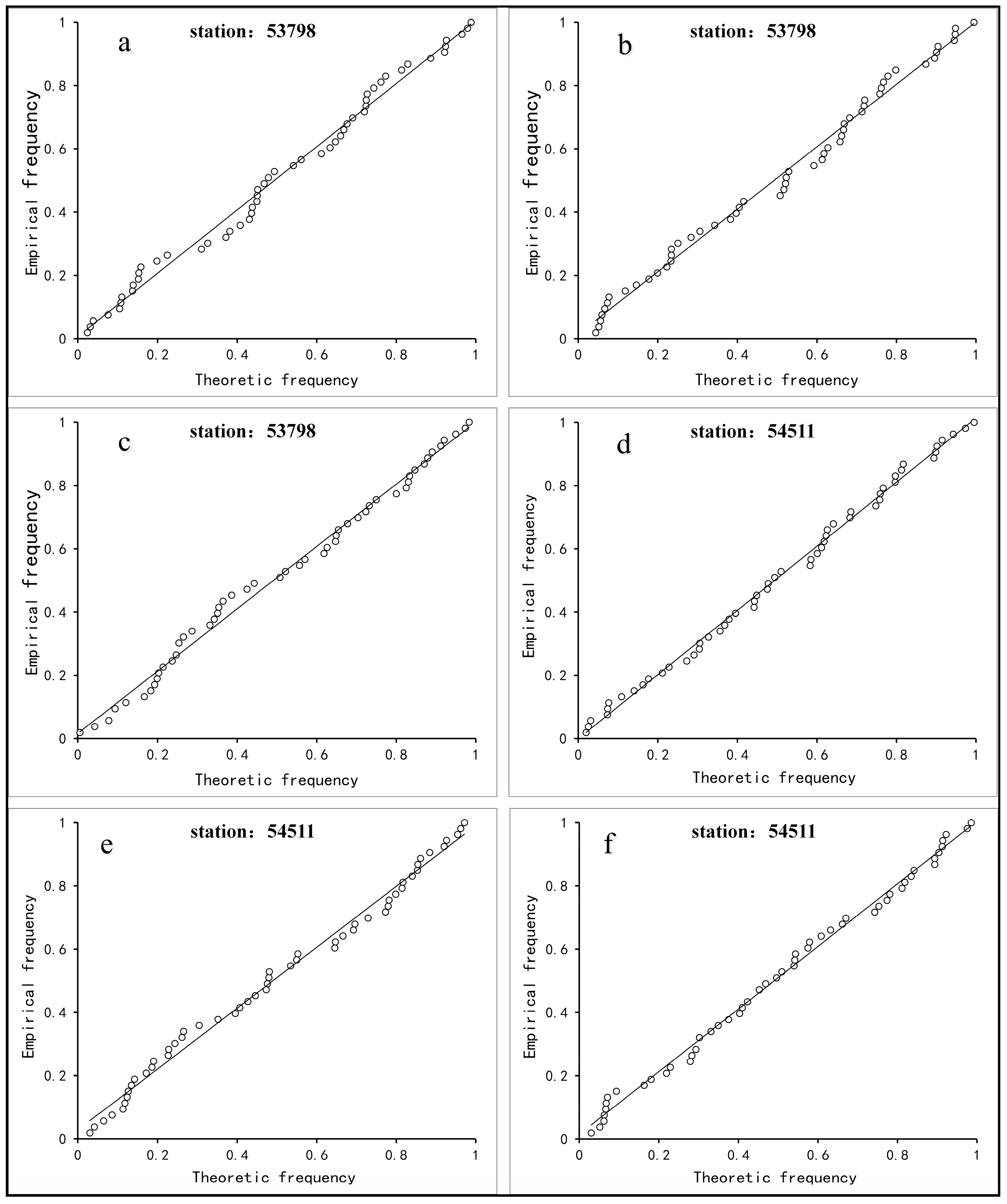
K-S test method [36] is used to verify the distance DI between empirical distribution function F_n(x) and hypothetic overall distribution function F₀(x). DI is calculated as follows:

$$DI=\underset{-\infty <x<\infty }{\sup }\left|F_n\left(x\right)-F_0\left(x\right)\right|$$

(13)

3.5.2. Graphic Test

This method gives intuitive description of the goodness of fit through graphics. Theoretical joint probability and empirical joint probability are indicated in a scatter diagram. If the pitches are evenly distributed in the vicinity of 45° line, it means the joint probability distribution model built is reasonable. Bivariate empirical joint probability distribution is calculated as follows [34]:

$$F_{emp}\left(x_{i1},x_{i2}\right)=p\left(X\le x_{i1},X\le x_{i2}\right)=\left({\displaystyle \sum _{g=1}^n{\displaystyle \sum _{k=1}^n{n}_{g,k}-0.44}}\right)/\left(n+0.12\right)$$

(14)

where, F_emp means empirical joint probability distribution; n_g,k represents the number of joint observations that satisfy X ≤ x_i1, X ≤ x_i2; n stands for sequences length.

4. Results and Discussion

4.1. Seasonal Distribution of Regional Precipitation

This paper makes statistics of the mean annual precipitation and its seasonal distribution (Table 3) observed at each meteorological station on the NCP from 1960 to 2012. According to the results, summer contributed the major part of precipitation on the NCP, which accounted for 56.45%–72.02% of mean annual precipitation. The precipitation in autumn and spring came the second. Winter precipitation was the smallest (less than 4%). Meanwhile, it is hardly that the drought or flood events happen in winter according to the statistical results of historical drought and flood events in the Haihe River Basin [22]. Therefore, this paper principally addresses the characteristics of DFCEs in spring, summer and autumn.

Table 3. Seasonal distribution of mean annual precipitation at meteorological stations in NCP.

Sub-Region	Meteorological Stations	Mean Annual Precipitation/mm	Seasonal Distribution of Precipitation/%
			Spring	Summer	Autumn	Winter
I	53798	516	13.72	64.61	18.81	2.86
	53898	561	14.64	62.56	19.43	3.36
	53986	567	15.88	60.33	20.71	3.09
	54727	637	15.14	63.69	17.93	3.24
	57091	630	17.92	56.45	21.35	4.28
	54705	479	14.07	63.95	18.79	3.19
	54511	556	11.74	71.72	14.68	1.86
II	54534	611	11.87	71.60	14.53	2.00
	54602	518	11.76	70.24	15.92	2.08
	54606	521	12.14	69.01	16.40	2.45
	54449	644	12.82	70.74	14.74	1.70
	54518	514	10.58	72.08	15.46	1.88
	54525	586	10.40	73.07	14.79	1.74
	54527	540	11.87	71.20	14.92	2.01
	54535	611	11.79	72.02	14.13	2.06
	54539	610	12.93	70.67	14.27	2.13
	54623	582	11.40	71.51	14.95	2.14
	54624	591	11.70	71.73	14.34	2.23
	54725	572	13.34	67.70	15.94	3.02

Table 3. Seasonal distribution of mean annual precipitation at meteorological stations in NCP.

Sub-Region	Meteorological Stations	Mean Annual Precipitation/mm	Seasonal Distribution of Precipitation/%
			Spring	Summer	Autumn	Winter
I	53798	516	13.72	64.61	18.81	2.86
	53898	561	14.64	62.56	19.43	3.36
	53986	567	15.88	60.33	20.71	3.09
	54727	637	15.14	63.69	17.93	3.24
	57091	630	17.92	56.45	21.35	4.28
	54705	479	14.07	63.95	18.79	3.19
	54511	556	11.74	71.72	14.68	1.86
II	54534	611	11.87	71.60	14.53	2.00
	54602	518	11.76	70.24	15.92	2.08
	54606	521	12.14	69.01	16.40	2.45
	54449	644	12.82	70.74	14.74	1.70
	54518	514	10.58	72.08	15.46	1.88
	54525	586	10.40	73.07	14.79	1.74
	54527	540	11.87	71.20	14.92	2.01
	54535	611	11.79	72.02	14.13	2.06
	54539	610	12.93	70.67	14.27	2.13
	54623	582	11.40	71.51	14.95	2.14
	54624	591	11.70	71.73	14.34	2.23
	54725	572	13.34	67.70	15.94	3.02

4.2. Results of Homogenous Regional Identification Based on L-moments

Four indicators of 19 meteorological stations on the NCP, including longitude, latitude, elevation and mean annual precipitation, are selected to identify the potential homogenous sub-region through K-Means cluster analysis. The regionalization results are shown in Figure 2. Discordancy test is performed respectively on the chosen seasonal precipitation (seasonal precipitation refers to the sum of precipitation of the three months in each season) of spring, summer and autumn at meteorological stations of each sub-region. This paper works out regional heterogeneity measure using Equations (7) and (8) through 1000 cycles of Monte Carlo simulation to test the regional heterogeneity. Finally, best-fit distribution functions are screened, including Generalized Extreme-Value (GEV), Generalized Logistic (GLO), Generalized Normal (GNO), Generalized Pareto (GPA), and Pearson III (P-III) [29,37]. Results of regional discordancy test, heterogeneity test and best-fit distribution function screening are shown in Table 4, Table 5 and Table 6, respectively.

As shown in Figure 2, the NCP is divided into two sub-regions. Sub-region I and sub-region II have 6 and 13 meteorological stations, respectively. The critical values of discordancy measure D are respectively 1.648 and 2.869 in sub-region I and II. As can be seen from Table 4, the discordancy measure D of meteorological stations in both sub-region I and sub-region II is smaller than respective critical values, which indicates that there is no singular station.

Figure 2. Identification of homogenous sub-regions in the NCP.

Figure 2. Identification of homogenous sub-regions in the NCP.

Table 4. Results of region-specific seasonal precipitation discordancy measure D.

Sub-Region I				Sub-Region II
Meteorological Stations	Discordancy Measure D			Meteorological Stations	Discordancy Measure D
	Spring	Summer	Autumn		Spring	Summer	Autumn
53798	1.08	1.47	0.36	54511	0.62	1.12	1.15
				54534	2.03	1.32	0.15
53898	1.64	0.1	0.95	54602	2.07	2.69	1.40
				54606	0.8	0.16	0.56
53986	0.81	0.22	0.95	54449	0.49	0.66	0.43
				54518	0.09	1.46	2.11
54727	1.32	1.64	1.13	54525	0.94	0.57	1.50
				54527	0.29	0.41	0.75
57091	0.48	1.61	1.38	54535	0.67	0.09	1.05
				54539	0.34	0.41	1.72
54705	0.65	0.95	1.25	54623	0.45	0.42	1.61
				54624	1.92	2.02	0.20
				54725	2.30	1.68	0.36

Table 4. Results of region-specific seasonal precipitation discordancy measure D.

Sub-Region I				Sub-Region II
Meteorological Stations	Discordancy Measure D			Meteorological Stations	Discordancy Measure D
	Spring	Summer	Autumn		Spring	Summer	Autumn
53798	1.08	1.47	0.36	54511	0.62	1.12	1.15
				54534	2.03	1.32	0.15
53898	1.64	0.1	0.95	54602	2.07	2.69	1.40
				54606	0.8	0.16	0.56
53986	0.81	0.22	0.95	54449	0.49	0.66	0.43
				54518	0.09	1.46	2.11
54727	1.32	1.64	1.13	54525	0.94	0.57	1.50
				54527	0.29	0.41	0.75
57091	0.48	1.61	1.38	54535	0.67	0.09	1.05
				54539	0.34	0.41	1.72
54705	0.65	0.95	1.25	54623	0.45	0.42	1.61
				54624	1.92	2.02	0.20
				54725	2.30	1.68	0.36

Table 5. Results of regional heterogeneity measure H.

Sub-Region	Seasons	Heterogeneity Measure
		H1	H2	H3
I	Spring	0.86	−0.88	−1.69
	Summer	0.41	0.23	0.44
	Autumn	−0.23	−1.03	−0.88
II	Spring	−1.01	−2.10	−2.54
	Summer	−0.25	0.24	0.10
	Autumn	−1.85	−2.24	−1.54

Table 5. Results of regional heterogeneity measure H.

Sub-Region	Seasons	Heterogeneity Measure
		H1	H2	H3
I	Spring	0.86	−0.88	−1.69
	Summer	0.41	0.23	0.44
	Autumn	−0.23	−1.03	−0.88
II	Spring	−1.01	−2.10	−2.54
	Summer	−0.25	0.24	0.10
	Autumn	−1.85	−2.24	−1.54

Table 6. Calculation of statistics Z^DIST for distribution fitting function of seasonal precipitation within sub-region.

Sub-Region	Distribution	Spring	Summer	Autumn
I	GLO	2.11	1.00	4.15
	GEV	0.59	−1.50	2.38
	GNO	0.14	−1.25	1.87
	P-III	−0.75	−1.45	0.87
	GPA	−3.01	−6.48	−1.81
II	GLO	4.13	5.84	2.15
	GEV	1.76	2.07	−0.48
	GNO	1.11	2.16	−0.79
	P-III	−0.20	1.59	−1.64
	GPA	−3.81	−5.75	−6.30
Best fit	Sub-region I	GNO	GLO	P-III
	Sub-region II	P-III	P-III	GEV

Table 6. Calculation of statistics Z^DIST for distribution fitting function of seasonal precipitation within sub-region.

Sub-Region	Distribution	Spring	Summer	Autumn
I	GLO	2.11	1.00	4.15
	GEV	0.59	−1.50	2.38
	GNO	0.14	−1.25	1.87
	P-III	−0.75	−1.45	0.87
	GPA	−3.01	−6.48	−1.81
II	GLO	4.13	5.84	2.15
	GEV	1.76	2.07	−0.48
	GNO	1.11	2.16	−0.79
	P-III	−0.20	1.59	−1.64
	GPA	−3.81	−5.75	−6.30
Best fit	Sub-region I	GNO	GLO	P-III
	Sub-region II	P-III	P-III	GEV

According to the result of regional heterogeneity test (Table 5), the values of heterogeneity measure H for sub-region I and sub-region II in spring, summer and autumn are all smaller than 1, which meets the consistency test requirement. Therefore, it is reasonable that the meteorological stations of sub-region I and sub-region II are regarded as being in one region, respectively.

Figure 3. The comparison between empirical frequency and the best-fit distributions’ theoretical frequency of seasonal precipitation at meteorological stations 53798 and 54511 (station 53798: (a) for spring; (b) for summer and (c) for autumn; station 54511: (d) for spring; (e) for summer; (f) for autumn.).

Figure 3. The comparison between empirical frequency and the best-fit distributions’ theoretical frequency of seasonal precipitation at meteorological stations 53798 and 54511 (station 53798: (a) for spring; (b) for summer and (c) for autumn; station 54511: (d) for spring; (e) for summer; (f) for autumn.).

The statistics values Z^DIST are calculated for distribution GLO, GEV, GNO, P-III and GPA in spring, summer and autumn, respectively. The results (Table 6) are shown that the best distribution fitting functions for spring, summer and autumn in sub-region I are GNO, GLO and P-III distributions, respectively. In sub-region II, the best distribution fitting functions for spring, summer and autumn are respectively P-III, P-III and GEV.

Besides, this paper compares the empirical frequency with the best-fit distributions’ theoretical frequency of seasonal precipitation in spring, summer and autumn at each meteorological station through graphic test. Figure 3 further demonstrates that the selected best-fit distributions are reasonable.

Figure 4. The comparison between empirical frequency and the best-fit distributions’ theoretical frequency of precipitation anomaly percentage at meteorological stations 53798 and 54511 (station 53798: (a) for spring; (b) for summer and (c) for autumn; station 54511: (d) for spring; (e) for summer and (f) for autumn).

Figure 4. The comparison between empirical frequency and the best-fit distributions’ theoretical frequency of precipitation anomaly percentage at meteorological stations 53798 and 54511 (station 53798: (a) for spring; (b) for summer and (c) for autumn; station 54511: (d) for spring; (e) for summer and (f) for autumn).

Table 7. Parameter estimates and K-S test values of the best-fit distribution for precipitation anomaly percentage in spring, summer and autumn in NCP.

Seasons			Spring				Summer				Autumn
Sub-region I	Best-fit distribution		GNO				GLO				P-III
	Parameter/Statistic		ξ	α	k	K-S	ξ	α	k	K-S	ξ	β	α	K-S
	Meteorological stations	53798	−18.0588	58.4344	−0.5694	0.0688	−9.1975	21.9138	−0.2385	0.0550	−139.5923	0.0373	5.2070	0.0693
		53898	−9.2467	48.2550	−0.3702	0.0565	−3.8273	21.4678	−0.1070	0.0563	−182.1496	0.0471	8.5867	0.1006
		53986	−11.1264	47.9706	−0.4416	0.0759	−3.5532	21.7771	−0.0981	0.0645	−145.0157	0.0408	5.9120	0.0830
		54727	−9.1277	51.0613	−0.3469	0.0712	−0.5261	18.1884	−0.0176	0.0653	−100.7213	0.0247	2.4881	0.0898
		57091	−12.3213	50.2480	−0.4644	0.0337	−0.9850	21.1229	−0.0283	0.0715	−146.8917	0.0535	7.8616	0.0890
		54705	−14.4809	57.8962	−0.4728	0.0697	−1.6266	20.8702	−0.0472	0.0797	−103.6220	0.0219	2.2695	0.0649
Sub-region II	Best-fit distribution		P-III				P-III				GEV
	Parameter/ Statistic		ξ	β	α	K-S	ξ	β	α	K-S	ξ	α	k	K-S
	Meteorological stations	54511	−88.8633	0.0227	2.0169	0.0507	−373.1322	0.2892	107.9153	0.0743	−23.3955	48.5116	0.1051	0.0614
		54534	−104.9823	0.0384	4.0270	0.0559	−207.6734	0.2079	43.1766	0.0677	−24.5054	41.0608	−0.0195	0.0506
		54602	−88.1920	0.0179	1.5810	0.0603	−159.0345	0.0771	12.2663	0.0863	−27.3803	42.1948	−0.0679	0.0584
		54606	−123.6783	0.0317	3.9160	0.0551	−177.7901	0.1282	22.7881	0.0561	−23.6675	44.2714	0.0448	0.0644
		54449	−127.4946	0.0452	5.7573	0.0413	−75.7425	0.0524	3.9695	0.0600	−23.7160	38.0654	−0.0444	0.0557
		54518	−126.5779	0.0397	5.0303	0.0473	−87.5464	0.0524	4.5891	0.0600	−28.1047	47.1006	−0.0194	0.0419
		54525	−120.2312	0.0368	4.4193	0.0403	−220.0703	0.1549	34.0958	0.0712	−22.4098	47.3171	0.1156	0.0688
		54527	−123.3882	0.0409	5.0426	0.0598	−153.9328	0.1290	19.8613	0.0660	−22.1711	41.8291	0.0499	0.0746
		54535	−89.4351	0.0222	1.9896	0.0638	−142.8562	0.1001	14.3053	0.0729	−23.4979	35.9935	−0.0714	0.0661
		54539	−104.3600	0.0304	3.1702	0.0797	−150.9863	0.1161	17.5369	0.0731	−23.2573	40.0777	−0.0031	0.0918
		54623	−125.3790	0.0322	4.0405	0.0458	−94.3140	0.0638	6.0195	0.0824	−24.5883	39.9580	−0.0372	0.0689
		54624	−128.0802	0.0353	4.5151	0.0886	−88.6065	0.0532	4.7131	0.0616	−24.0894	39.3210	−0.0347	0.0506
		54725	−144.6437	0.0514	7.4316	0.0755	−82.7962	0.0570	4.7227	0.0595	−22.4426	40.9570	0.0304	0.0703

Table 7. Parameter estimates and K-S test values of the best-fit distribution for precipitation anomaly percentage in spring, summer and autumn in NCP.

Seasons			Spring				Summer				Autumn
Sub-region I	Best-fit distribution		GNO				GLO				P-III
	Parameter/Statistic		ξ	α	k	K-S	ξ	α	k	K-S	ξ	β	α	K-S
	Meteorological stations	53798	−18.0588	58.4344	−0.5694	0.0688	−9.1975	21.9138	−0.2385	0.0550	−139.5923	0.0373	5.2070	0.0693
		53898	−9.2467	48.2550	−0.3702	0.0565	−3.8273	21.4678	−0.1070	0.0563	−182.1496	0.0471	8.5867	0.1006
		53986	−11.1264	47.9706	−0.4416	0.0759	−3.5532	21.7771	−0.0981	0.0645	−145.0157	0.0408	5.9120	0.0830
		54727	−9.1277	51.0613	−0.3469	0.0712	−0.5261	18.1884	−0.0176	0.0653	−100.7213	0.0247	2.4881	0.0898
		57091	−12.3213	50.2480	−0.4644	0.0337	−0.9850	21.1229	−0.0283	0.0715	−146.8917	0.0535	7.8616	0.0890
		54705	−14.4809	57.8962	−0.4728	0.0697	−1.6266	20.8702	−0.0472	0.0797	−103.6220	0.0219	2.2695	0.0649
Sub-region II	Best-fit distribution		P-III				P-III				GEV
	Parameter/ Statistic		ξ	β	α	K-S	ξ	β	α	K-S	ξ	α	k	K-S
	Meteorological stations	54511	−88.8633	0.0227	2.0169	0.0507	−373.1322	0.2892	107.9153	0.0743	−23.3955	48.5116	0.1051	0.0614
		54534	−104.9823	0.0384	4.0270	0.0559	−207.6734	0.2079	43.1766	0.0677	−24.5054	41.0608	−0.0195	0.0506
		54602	−88.1920	0.0179	1.5810	0.0603	−159.0345	0.0771	12.2663	0.0863	−27.3803	42.1948	−0.0679	0.0584
		54606	−123.6783	0.0317	3.9160	0.0551	−177.7901	0.1282	22.7881	0.0561	−23.6675	44.2714	0.0448	0.0644
		54449	−127.4946	0.0452	5.7573	0.0413	−75.7425	0.0524	3.9695	0.0600	−23.7160	38.0654	−0.0444	0.0557
		54518	−126.5779	0.0397	5.0303	0.0473	−87.5464	0.0524	4.5891	0.0600	−28.1047	47.1006	−0.0194	0.0419
		54525	−120.2312	0.0368	4.4193	0.0403	−220.0703	0.1549	34.0958	0.0712	−22.4098	47.3171	0.1156	0.0688
		54527	−123.3882	0.0409	5.0426	0.0598	−153.9328	0.1290	19.8613	0.0660	−22.1711	41.8291	0.0499	0.0746
		54535	−89.4351	0.0222	1.9896	0.0638	−142.8562	0.1001	14.3053	0.0729	−23.4979	35.9935	−0.0714	0.0661
		54539	−104.3600	0.0304	3.1702	0.0797	−150.9863	0.1161	17.5369	0.0731	−23.2573	40.0777	−0.0031	0.0918
		54623	−125.3790	0.0322	4.0405	0.0458	−94.3140	0.0638	6.0195	0.0824	−24.5883	39.9580	−0.0372	0.0689
		54624	−128.0802	0.0353	4.5151	0.0886	−88.6065	0.0532	4.7131	0.0616	−24.0894	39.3210	−0.0347	0.0506
		54725	−144.6437	0.0514	7.4316	0.0755	−82.7962	0.0570	4.7227	0.0595	−22.4426	40.9570	0.0304	0.0703

4.3. Parameter Estimation and Goodness of Fit Test of the Best-Fit Distribution

According to Equation (11), the precipitation anomaly percentage and precipitation of a certain period are subject to the same distribution, so the fitting is possible with the same distribution fitting function. Therefore, the precipitation anomaly percentages in spring, summer and autumn are fitted with GNO, GLO and P-III distributions in sub-region I, respectively. In sub-region II, the precipitation anomaly percentages in spring, summer and autumn are, respectively, fitted with P-III, P-III and GEV. Moreover, the parameters of each distribution are estimated by L-moments method. Goodness of fit test is performed on each distribution by K-S method with statistically significance (α = 0.05, n = 53, D < 1.87). The results of parameter estimation and K-S test are shown in Table 7. Furthermore, this paper uses the graphic test again to compare the empirical frequency with the best-fit distributions’ theoretical frequency of precipitation anomaly percentage in spring, summer and autumn at each meteorological station. Figure 4 further demonstrates that the selected best-fit distributions are reasonable.

4.4. Bivariate Copula Distribution Parameter Estimation and Fitting Test

For the precipitation anomaly percentage sequence in spring, summer and autumn at meteorological stations in each sub-region, this paper works out Kendall rank correlation coefficient τ with Equation (12), and estimates the parameter θ in bivariate Gumbel copula, Clayton copula, and Frank copula distribution functions based on the relation between θ and τ as shown in Table 2. By comparing the calculated value and its value range of parameter θ, Frank copula is suitable for using by the positive and negative correlation. Hence, this paper seeks the probability of seasonal DFCEs only through Frank copula distribution function. Refer to Table 8 for the Kendall rank correlation coefficient τ and the parameter θ of spring-summer and summer-autumn precipitation anomaly percentage sequence, as well as the results of K-S test. As shown in Table 8, K-S test has passed α=0.05 significance test (n = 53, D < 1.87). Furthermore, this paper compares the spring-summer and summer-autumn empirical frequency at each meteorological station with the theoretical frequency of Frank copula distribution through graphic test. Figure 5 further demonstrates that the selected Frank copula distribution function is reasonable.

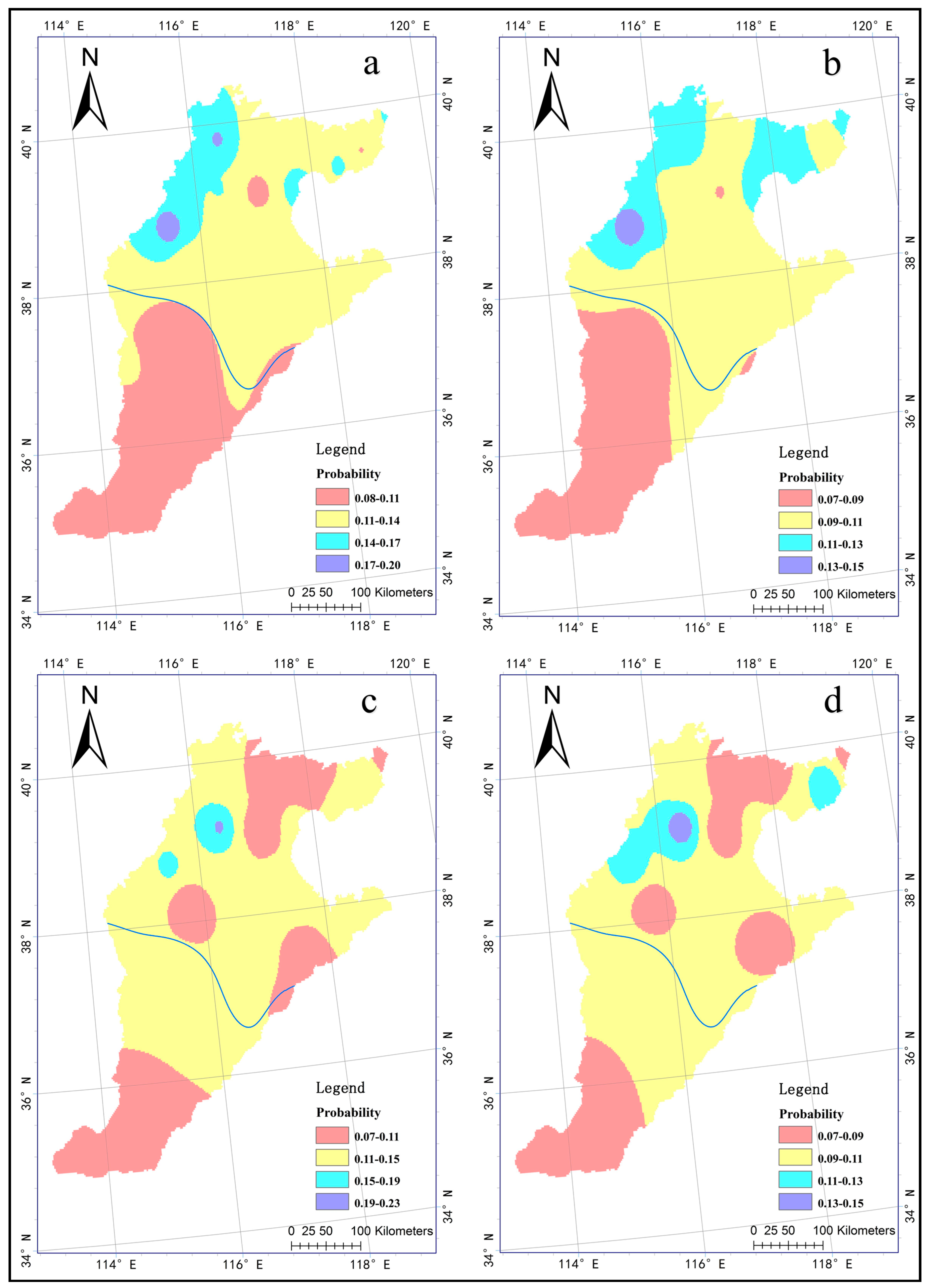
4.5. Analysis of the Occurrence Frequency of DFCEs

According to the two inquations Pa < −25% and Pa > 25%, the precipitations of spring, summer and autumn at each station are divided into “drought”, “normal” and “flood” states based on single-station drought & flood indicators division criteria (Table 9) [38]. As shown in Table 9, Pa < −25% means “drought”; −25% ≤ Pa < 25% stands for “normal”; Pa ≥ 25% represents “flood”. DFCEs between seasons could be divided into the following 4 categories (X and Y respectively refer to the spring-summer or summer-autumn precipitation anomaly percentages at a certain meteorological station).

Figure 5. The comparison between empirical frequency and the theoretical frequency of Frank copula distribution at meteorological station 53798 and 54511 (station 53798: (a) for spring-summer; (b) for summer-autumn; Station 54511: (c) for spring-summer; (d) for summer-autumn).

Figure 5. The comparison between empirical frequency and the theoretical frequency of Frank copula distribution at meteorological station 53798 and 54511 (station 53798: (a) for spring-summer; (b) for summer-autumn; Station 54511: (c) for spring-summer; (d) for summer-autumn).

Table 8. Computation of Kendall rank correlation coefficient τ, parameter θ and K-S test in spring-summer and summer-autumn.

Sub-Regions	Meteorological Stations	Spring-Summer			Summer-Autumn
		τ	θ	K-S	τ	θ	K-S
I	53798	−0.1176	−1.0701	0.1010	0.0261	0.2354	0.0633
	53898	−0.0225	−0.2026	0.0893	−0.0530	−0.4780	0.1352
	53986	0.0094	0.0849	0.1025	−0.0290	−0.2616	0.0691
	54727	0.0261	0.2353	0.0728	0.0987	0.8953	0.0750
	57091	−0.0044	−0.0392	0.0835	0.0225	0.2026	0.1053
	54705	−0.1001	−0.9087	0.0604	0.0290	0.2616	0.0802
II	54511	0.0624	0.5635	0.0901	−0.0131	−0.1177	0.0617
	54534	0.1713	1.5792	0.0814	−0.0377	−0.3400	0.0886
	54602	0.1046	0.9496	0.0842	0.1089	0.9892	0.0667
	54606	0.0203	0.1829	0.0606	−0.0690	−0.6231	0.0611
	54449	0.1880	1.7425	0.0697	−0.0566	−0.5108	0.1033
	54518	0.0639	0.5771	0.0563	0.2890	2.7943	0.0607
	54525	0.0501	0.4521	0.0643	−0.0298	−0.2681	0.0883
	54527	0.0124	0.1112	0.0941	−0.0145	−0.1306	0.0969
	54535	0.1147	1.0431	0.0734	0.1220	1.1115	0.0758
	54539	0.0145	0.1306	0.0554	0.2395	2.2619	0.1014
	54623	0.1611	1.4813	0.0818	0.0726	0.6559	0.0669
	54624	−0.0065	−0.0588	0.0758	0.0363	0.3269	0.0903
	54725	0.0922	0.8355	0.0643	0.0276	0.2483	0.0842

Table 8. Computation of Kendall rank correlation coefficient τ, parameter θ and K-S test in spring-summer and summer-autumn.

Sub-Regions	Meteorological Stations	Spring-Summer			Summer-Autumn
		τ	θ	K-S	τ	θ	K-S
I	53798	−0.1176	−1.0701	0.1010	0.0261	0.2354	0.0633
	53898	−0.0225	−0.2026	0.0893	−0.0530	−0.4780	0.1352
	53986	0.0094	0.0849	0.1025	−0.0290	−0.2616	0.0691
	54727	0.0261	0.2353	0.0728	0.0987	0.8953	0.0750
	57091	−0.0044	−0.0392	0.0835	0.0225	0.2026	0.1053
	54705	−0.1001	−0.9087	0.0604	0.0290	0.2616	0.0802
II	54511	0.0624	0.5635	0.0901	−0.0131	−0.1177	0.0617
	54534	0.1713	1.5792	0.0814	−0.0377	−0.3400	0.0886
	54602	0.1046	0.9496	0.0842	0.1089	0.9892	0.0667
	54606	0.0203	0.1829	0.0606	−0.0690	−0.6231	0.0611
	54449	0.1880	1.7425	0.0697	−0.0566	−0.5108	0.1033
	54518	0.0639	0.5771	0.0563	0.2890	2.7943	0.0607
	54525	0.0501	0.4521	0.0643	−0.0298	−0.2681	0.0883
	54527	0.0124	0.1112	0.0941	−0.0145	−0.1306	0.0969
	54535	0.1147	1.0431	0.0734	0.1220	1.1115	0.0758
	54539	0.0145	0.1306	0.0554	0.2395	2.2619	0.1014
	54623	0.1611	1.4813	0.0818	0.0726	0.6559	0.0669
	54624	−0.0065	−0.0588	0.0758	0.0363	0.3269	0.0903
	54725	0.0922	0.8355	0.0643	0.0276	0.2483	0.0842

Table 9. Drought & flood grade standard of precipitation anomaly percentage (M).

Grade	Anomaly Percentage	Type of Drought & Flood
1	M ≥ 75%	Serious flood
2	50% ≤ M < 75%	Heavy flood
3	25% ≤ M < 50%	Relatively heavy flood
4	−25% ≤ M < 25%	Normal
5	−50% ≤ M < −25%	Relatively heavy drought
6	−75% ≤ M < −50%	Heavy drought
7	M < −75%	Serious drought

Table 9. Drought & flood grade standard of precipitation anomaly percentage (M).

Grade	Anomaly Percentage	Type of Drought & Flood
1	M ≥ 75%	Serious flood
2	50% ≤ M < 75%	Heavy flood
3	25% ≤ M < 50%	Relatively heavy flood
4	−25% ≤ M < 25%	Normal
5	−50% ≤ M < −25%	Relatively heavy drought
6	−75% ≤ M < −50%	Heavy drought
7	M < −75%	Serious drought

Continuous drought in spring-summer (SSD)/continuous drought in summer-autumn (SAD):

P_dro-dro=P(X < −25%, Y < −25%);

Spring drought & summer flood (SDSF)/ summer flood & autumn drought (SDAF):

P_dro-flo=P(X < −25%, Y ≥ 25%);

Spring flood & summer drought (SFSD)/ summer flood & autumn drought (SFAD):

P_flo-dro=P(X ≥ −25%, Y < 25%);

Continuous flood in spring-summer (SSF)/ continuous flood in summer-autumn (SAF):

P_flo-flo=P(X ≥ 25%, Y ≥ 25%).

The frequency of above-noted 4 DFCEs is figured out based on the anomaly percentage marginal distribution of seasonal precipitation and the Frank copula joint distribution between seasons (see Table 10). As shown in Table 10:

Table 10. Computed result of joint distribution of DFCEs on the NCP.

Sub-Region	Meteorological Stations	Seasonal Drought & Flood Joint Distribution Probability								Probability of Spring-Summer DFCEs	Probability of Summer-Autumn DFCEs
		SSD	SDSF	SFSD	SSF	SAD	SDAF	SFAD	SAF
I	53798	0.1128	0.0732	0.0624	0.0401	0.1340	0.0944	0.0907	0.0640	0.2885	0.3831
	53898	0.0904	0.0767	0.0651	0.0553	0.0970	0.0659	0.0820	0.0557	0.2875	0.3006
	53986	0.1011	0.0871	0.0691	0.0596	0.1016	0.0682	0.0872	0.0585	0.3169	0.3155
	54727	0.0802	0.0786	0.0597	0.0586	0.1039	0.0719	0.1020	0.0706	0.2771	0.3484
	57091	0.0935	0.0898	0.0620	0.0595	0.0905	0.0705	0.0869	0.0677	0.3048	0.3156
	54705	0.0823	0.0765	0.0508	0.0472	0.1173	0.0700	0.1097	0.0655	0.2568	0.3625
II	54511	0.1727	0.1269	0.1190	0.0877	0.1313	0.1084	0.0946	0.0780	0.5063	0.4123
	54534	0.1174	0.1115	0.0859	0.0817	0.0746	0.0530	0.0704	0.0500	0.3965	0.2480
	54602	0.1832	0.1419	0.1128	0.0880	0.1578	0.1103	0.1227	0.0862	0.5259	0.4770
	54606	0.1208	0.1055	0.0792	0.0691	0.0833	0.0633	0.0720	0.0547	0.3746	0.2733
	54449	0.1451	0.1217	0.1106	0.0932	0.0868	0.0599	0.0708	0.0487	0.4706	0.2662
	54518	0.1406	0.1020	0.1015	0.0738	0.1946	0.1495	0.1461	0.1141	0.4179	0.6043
	54525	0.1157	0.1044	0.0857	0.0774	0.0884	0.0737	0.0793	0.0661	0.3832	0.3075
	54527	0.0969	0.0885	0.0702	0.0641	0.0820	0.0640	0.0748	0.0584	0.3197	0.2792
	54535	0.1437	0.1247	0.0968	0.0842	0.1232	0.0877	0.1071	0.0765	0.4494	0.3945
	54539	0.1096	0.0977	0.0731	0.0652	0.1406	0.1101	0.1270	0.0998	0.3456	0.4775
	54623	0.1584	0.1267	0.1135	0.0914	0.1216	0.0878	0.0963	0.0698	0.4900	0.3755
	54624	0.1177	0.0905	0.0880	0.0677	0.1176	0.0844	0.0912	0.0656	0.3639	0.3588
	54725	0.1316	0.1014	0.0978	0.0756	0.1072	0.0828	0.0817	0.0632	0.4064	0.3349

Table 10. Computed result of joint distribution of DFCEs on the NCP.

Sub-Region	Meteorological Stations	Seasonal Drought & Flood Joint Distribution Probability								Probability of Spring-Summer DFCEs	Probability of Summer-Autumn DFCEs
		SSD	SDSF	SFSD	SSF	SAD	SDAF	SFAD	SAF
I	53798	0.1128	0.0732	0.0624	0.0401	0.1340	0.0944	0.0907	0.0640	0.2885	0.3831
	53898	0.0904	0.0767	0.0651	0.0553	0.0970	0.0659	0.0820	0.0557	0.2875	0.3006
	53986	0.1011	0.0871	0.0691	0.0596	0.1016	0.0682	0.0872	0.0585	0.3169	0.3155
	54727	0.0802	0.0786	0.0597	0.0586	0.1039	0.0719	0.1020	0.0706	0.2771	0.3484
	57091	0.0935	0.0898	0.0620	0.0595	0.0905	0.0705	0.0869	0.0677	0.3048	0.3156
	54705	0.0823	0.0765	0.0508	0.0472	0.1173	0.0700	0.1097	0.0655	0.2568	0.3625
II	54511	0.1727	0.1269	0.1190	0.0877	0.1313	0.1084	0.0946	0.0780	0.5063	0.4123
	54534	0.1174	0.1115	0.0859	0.0817	0.0746	0.0530	0.0704	0.0500	0.3965	0.2480
	54602	0.1832	0.1419	0.1128	0.0880	0.1578	0.1103	0.1227	0.0862	0.5259	0.4770
	54606	0.1208	0.1055	0.0792	0.0691	0.0833	0.0633	0.0720	0.0547	0.3746	0.2733
	54449	0.1451	0.1217	0.1106	0.0932	0.0868	0.0599	0.0708	0.0487	0.4706	0.2662
	54518	0.1406	0.1020	0.1015	0.0738	0.1946	0.1495	0.1461	0.1141	0.4179	0.6043
	54525	0.1157	0.1044	0.0857	0.0774	0.0884	0.0737	0.0793	0.0661	0.3832	0.3075
	54527	0.0969	0.0885	0.0702	0.0641	0.0820	0.0640	0.0748	0.0584	0.3197	0.2792
	54535	0.1437	0.1247	0.0968	0.0842	0.1232	0.0877	0.1071	0.0765	0.4494	0.3945
	54539	0.1096	0.0977	0.0731	0.0652	0.1406	0.1101	0.1270	0.0998	0.3456	0.4775
	54623	0.1584	0.1267	0.1135	0.0914	0.1216	0.0878	0.0963	0.0698	0.4900	0.3755
	54624	0.1177	0.0905	0.0880	0.0677	0.1176	0.0844	0.0912	0.0656	0.3639	0.3588
	54725	0.1316	0.1014	0.0978	0.0756	0.1072	0.0828	0.0817	0.0632	0.4064	0.3349

Figure 6. Spatial distribution of the probability of seasonal DFCEs on the NCP. (a,b) for continuous drought in spring-summer and spring drought & summer flood, respectively; (c,d) for continuous drought in summer-autumn and summer flood & autumn drought, respectively).

Figure 6. Spatial distribution of the probability of seasonal DFCEs on the NCP. (a,b) for continuous drought in spring-summer and spring drought & summer flood, respectively; (c,d) for continuous drought in summer-autumn and summer flood & autumn drought, respectively).

On the time scale, the analysis results are as follows:

(1) In sub-region I, SSD dominate in spring-summer DFCEs, and SDSF come second. The average probability values are 0.09 and 0.08, respectively. SAD prevail in summer-autumn DFCEs, and SFAD come next, which average probability values are respectively 0.11 and 0.09. While SDAF preponderate at meteorological station 53798; (2) SSD still dominate in spring-summer DFCEs in sub-region II, which average probability value is 0.13; SDSF come next with the average probability value 0.11. In summer-autumn DFCEs, SSD prevail over the other events with the average probability value 0.12; SDSF and SFSD come next, both of which average probability values are the same (0.09); (3) In sub-region I, the probability of spring-summer DFCEs is less than the summer-autumn DFCEs’, that means summer-autumn DFCEs prevail in this region. The probability of spring-summer DFCEs is greater than the summer-autumn DFCEs’ at most meteorological stations in sub-region II, which indicates spring-summer DFCEs dominate in this region.

On the spatial scale, the analysis results are as follows:

This paper uses Inverse Distance Weighting to analyze the occurrence frequency of DFCEs on the spatial scale (Figure 6). As shown in Figure 6a,b, SSD and SDSF most probably occur in the northwest and northeast as well as near the coastal areas of sub-region II. According to Figure 6c,d, the most probable events of SAD and SFAD occur in central area of northwestern part of sub-region II. Besides, the probability of occurrence of SFAD is also great in the northeast and near the coastal areas.

5. Conclusions

This paper has probed into the probability characteristics of DFCEs between seasons on the NCP by L-moments theory and bivariate copula distribution based on the daily precipitation data gathered in the period from 1960 to 2012 at 19 meteorological stations on the NCP. The principal research conclusions are as follows:

(1) According to the mean annual precipitation on the NCP, summer contributed the major part of precipitation and accounted for 56.45%–72.02%. The precipitation in autumn and spring came the second. Winter exhibited the lowest precipitation, which accounted for no more than 4%.

(2) The NCP is divided into two sub-regions. The best-fit distribution for precipitation anomaly percentages in the spring, summer and autumn at each meteorological station are GNO, GLO and P-III, respectively in sub-region I, and are P-III, P-III and GEV in sub-region II.

(3) Comparing to the Gumbel copula and Clayton copula, Frank copula is more suitable for the spring-summer and summer-autumn precipitation anomaly percentage sequences on the NCP. The fitting results have passed the K-S test and graphic test.

(4) On the time scale, SSD and SAD respectively dominate in spring-summer and summer-autumn DFCEs on the NCP. The average probability value (0.11) of SAD is greater in sub-region I, while the average probability value (0.12) of SAD is less than SAD’s. Furthermore, summer-autumn DFCEs prevail in sub-region I with the average probability value 0.34, while spring-summer DFCEs dominate in sub-region II, which average probability value is 0.42.

(5) On the spatial scale, SSD and SDSF most probably occur in the northwest and northeast as well as near the coastal areas of sub-region II, while SAD and SFAD most probably occur in central area of northwestern part of sub-region II.

This paper probes into the probability characteristics of DFCEs on the NCP from the perspective of meteorological drought & flood. It’s possible to use this method in subsequent researches to make further analysis of DFCEs from hydrological, agricultural and social perspectives, etc., so as to provide convincing reference frame for the comprehensive response to flood and drought disasters and water resource management.

References

1. IPCC. Climate Change 2007: Synthesis Report; Cambridge University Press: Cambridge, UK, 2007. [Google Scholar]
2. IPCC. Summary for Policymakers of Climate Change 2007: The Physical Science Basis. Contribution of Working Group I to the Fourth Assessment Report of the Intergovernmental Panel on Climate Change; Cambridge University Press: Cambridge, UK, 2007. [Google Scholar]
3. Shahabfar, A.; Eitzinger, J. Spatio-Temporal analysis of droughts in semi-arid regions by using meteorological drought indices. Atmosphere 2013, 4, 94–112. [Google Scholar] [CrossRef]
4. Liepert, B.G.; Romanou, A. Global dimming and brightening and the water cycle. Bull. Amer. Meteorol. Soc. 2005, 86, 622–623. [Google Scholar]
5. Wu, Z.W.; Li, J.P.; He, J.H.; Jiang, Z.H. Large-scale atmospheric singularities and summer long-cycle droughts-floods abrupt alternation in the middle and lower reaches of the Yangtze River. Chin. Sci. Bull. 2006, 51, 2027–2034. [Google Scholar] [CrossRef]
6. Wu, Z.W.; Li, J.P.; He, J.H.; Jiang, Z.H. Occurrence of droughts and floods during the normal summer monsoons in the mid- and lower reaches of the Yangtze River. Geophys. Res. Lett. 2006. [Google Scholar] [CrossRef]
7. Shiau, J.; Modarres, R. Copula-based drought severity-duration-frequency analysis in Iran. Meteorol. Appl. 2009, 16, 481–489. [Google Scholar] [CrossRef]
8. Ibrahim, K.; Wan Zin, W.Z.; Jemain, A.A. Evaluating the dry conditions in Peninsular Malaysia using bivariate copula. ANZIAM J. 2010, 51, C555–C569. [Google Scholar]
9. Mirabbasi, R.; Fakheri-Fard, A.; Dinpashoh, Y. Bivariate drought frequency analysis using the copula method. Theor. Appl. Climatol. 2012, 108, 191–206. [Google Scholar] [CrossRef]
10. Zhang, L.; Singh, V.P. Bivariate flood frequency analysis using the copula method. J. Hydrol. Eng. 2006, 11, 150–164. [Google Scholar] [CrossRef]
11. Sraj, M.; Bezak, N.; Brilly, M. Bivariate flood frequency analysis using the copula function: A case study of the Litija station on the Sava River. Hydrol. Process. 2014. [Google Scholar] [CrossRef]
12. Li, T.Y.; Guo, S.L.; Chen, L.; Guo, J. Bivariate flood frequency analysis with historical information based on copula. J. Hydrol. Eng. 2012, 18, 1018–1030. [Google Scholar] [CrossRef]
13. Mirabbasi, R.; Anagnostou, E.N.; Fakheri-Fard, A.; Dinpashoh, Y.; Eslamian, S. Analysis of meteorological drought in northwest Iran using the joint deficit index. J. Hydrol. 2013, 492, 35–48. [Google Scholar]
14. Madadgar, S.; Moradkhani, H. Drought analysis under climate change using copula. J. Hydrol. Eng. 2011, 18, 746–759. [Google Scholar] [CrossRef]
15. Ma, M.; Song, S.; Ren, L.; Jiang, S.; Song, J. Multivariate drought characteristics using trivariate Gaussian and Student copulas. Hydrol. Process. 2013, 27, 1175–1190. [Google Scholar] [CrossRef]
16. Zhang, L.; Singh, V.P. Trivariate flood frequency analysis using the Gumbel–Hougaard copula. J. Hydrol. Eng. 2007, 12, 431–439. [Google Scholar] [CrossRef]
17. Grimaldi, S.; Serinaldi, F. Asymmetric copula in multivariate flood frequency analysis. Adv. Water Resour. 2006, 29, 1155–1167. [Google Scholar] [CrossRef]
18. Serinaldi, F.; Kilsby, C.G. The intrinsic dependence structure of peak, volume, duration, and average intensity of hyetographs and hydrographs. Water Resour. Res. 2013, 49, 3423–3442. [Google Scholar] [CrossRef]
19. Bezak, N.; Mikoš, M.; Šraj, M. Trivariate frequency analyses of peak discharge, hydrograph volume and suspended sediment concentration data using copulas. Water Resour. Manag. 2014, 28, 2195–2212. [Google Scholar] [CrossRef]
20. Liu, C.M.; Yu, J.J.; Kendy, E. Groundwater exploitation and its impact on the environment in the North China Plain. Water Int. 2001, 26, 265–272. [Google Scholar] [CrossRef]
21. Ren, X.S. Water Resources Assessment of Haihe River Basin; China Water Power Press: Beijing, China, 1997. (in Chinese) [Google Scholar]
22. Haihe River Water Resources Conservancy Commission. Flood and Drought Disasters in Haihe River Basin; Tianjin Science and Technology Press: Tianjin, China, 2009. (in Chinese) [Google Scholar]
23. Committee for Haihe River Records Compilation. Haihe River Records (Volume One); China Water Power Press: Beijing, China, 1997. (in Chinese) [Google Scholar]
24. China Meteorological Data Sharing Service System. Available online: http://cdc.cma.gov.cn/home.do (accessed on 12 August 2014).
25. Qian, W.; Lin, X. Regional trends in recent precipitation indices in China. Meteorol. Atmos. Phys. 2005, 90, 193–207. [Google Scholar] [CrossRef]
26. Du, H.; Xia, J.; Zeng, S.D. Regional frequency analysis of extreme precipitation and its spatio-temporal characteristics in the Huai River Basin, China. Nat. Hazards 2014, 70, 195–215. [Google Scholar] [CrossRef]
27. Hosking, J.R.M. L-Moments: Analysis and estimation of distributions using linear combinations of order statistics. J. R. Stat. Soc. B 1990, 52, 105–124. [Google Scholar]
28. Sankarasubramanian, A.; Srinivasan, K. Investigation and comparison of sampling properties of L-moments and conventional moments. J. Hydrol. 1999, 218, 13–34. [Google Scholar] [CrossRef]
29. Hosking, J.R.M.; Wallis, J.R. Regional Frequency Analysis: An Approach Based on L-Moments; Cambridge University Press: Cambridge, UK, 1997. [Google Scholar]
30. Xiong, L.H.; Guo, S.L.; Wang, C.J. Advance in regional flood frequency analysis from abroad. Adv. Water Sci. 2004, 15, 261–267. (In Chinese) [Google Scholar]
31. Hosking, J.R.M.; Wallis, J.R. Some statistics useful in regional frequency analysis. Water Resour. Res. 1993, 29, 271–281. [Google Scholar] [CrossRef]
32. Norbiato, D.; Borga, M.; Sangati, M.; Zanon, F. Regional frequency analysis of extreme precipitation in the eastern Italian Alps and the August 29, 2003 flash flood. J. Hydrol. 2007, 345, 149–166. [Google Scholar] [CrossRef]
33. Shiau, J.T. Fitting drought duration and severity with two-dimensional copulas. Water Resour. Manag. 2006, 20, 795–815. [Google Scholar] [CrossRef]
34. Genest, C.; Rivest, L. Statistical inference procedures for bivariate Archimedean copulas. J. Am. Stat. Assoc. 1993, 88, 1034–1043. [Google Scholar] [CrossRef]
35. Kendall, M.G. A new measure of rank correlation. Biometrika. 1938, 30, 81–89. [Google Scholar] [CrossRef]
36. Massey, F.J., Jr. The Kolmogorov-Smirnov test for goodness of fit. J. Am. Stat. Assoc. 1951, 46, 68–78. [Google Scholar] [CrossRef]
37. Hosking, J.R.M. Research Report: Fortran Routines for Use with the Method of L-Moments, Version 3.04. Available online: http://btr0xq.rz.uni-bayreuth.de/math/statlib/general/lmoments.pdf (accessed on 13 November 2014).
38. Ju, X.S.; Yang, X.W.; Chen, L.J.; Wang, Y.M. Research on determination of station indexes and division of regional flood/drought grades in China. Q. J. Appl. Meteorol. 1997, 8, 26–33. (In Chinese) [Google Scholar]