
Airborne Aerosol in Situ Measurements during TCAP: A Closure Study of Total Scattering

 and
and
Abstract
:1. Introduction
- (1)
- What level of agreement can be achieved between the in-flight measured and calculated values of total scattering coefficient at ambient RH?
- (2)
- What is the effect of ignoring the influence of chemical composition data on this agreement?
- (3)
- How sensitive is this agreement to the assumed RI value, particularly if the assumed RI is non-representative of the ambient aerosol?
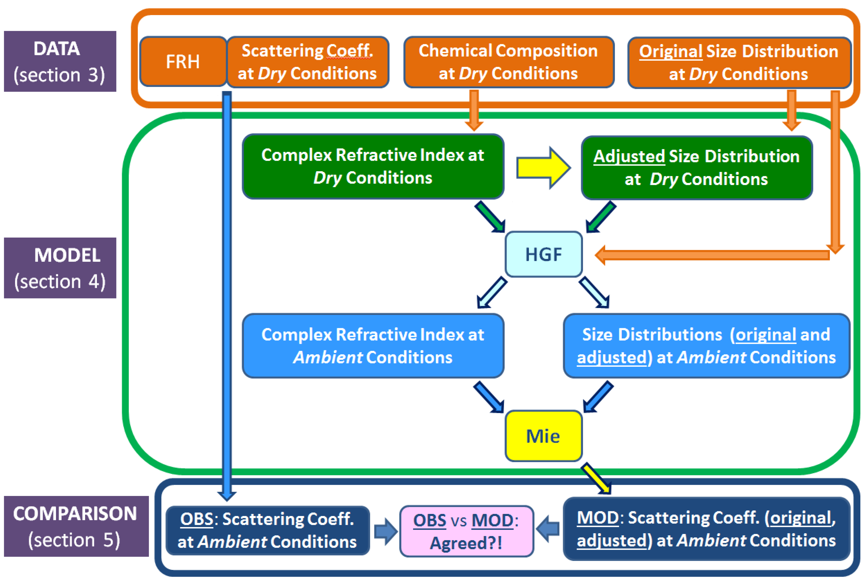
2. Approach

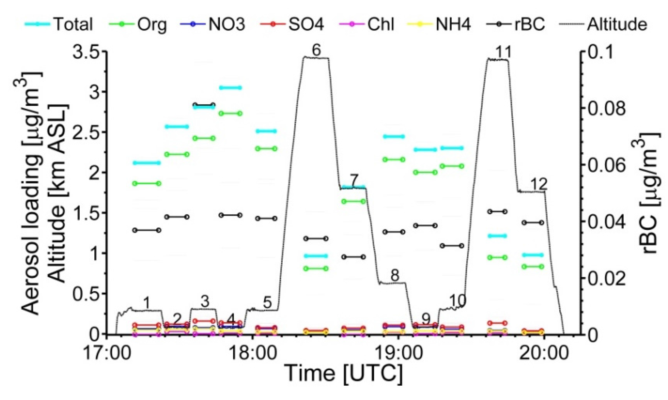
3. Data


4. Model and Adjustments
4.1. Hygroscopic Growth Factor

| OM | SO4 | NO3 | Chl | NH4 | BC | Water | |
|---|---|---|---|---|---|---|---|
| Density (g/cm3) | 1.4 | 1.8 | 1.8 | 1.53 | 1.8 | 1.8 | 1.0 |
| RI (real) | 1.45 | 1.52 | 1.5 | 1.64 | 1.5 | 1.85 | 1.33 |
| RI (imag) | 0.0 | 0 | 0 | 0 | 0 | 0.71 | 0 |
| HGF (RH = 80%) | 1.07 | 1.50 | 1.50 | 1.9 | 1.50 | 1.0 | - |

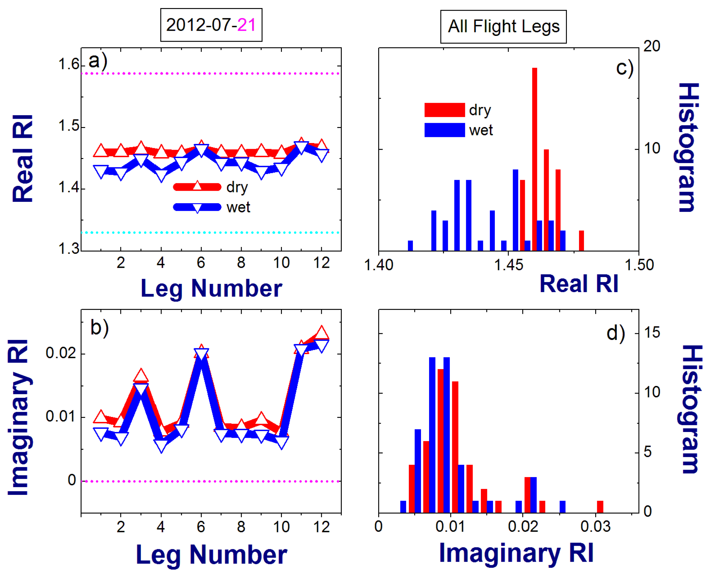
4.2. Dry and Wet Refractive Indices

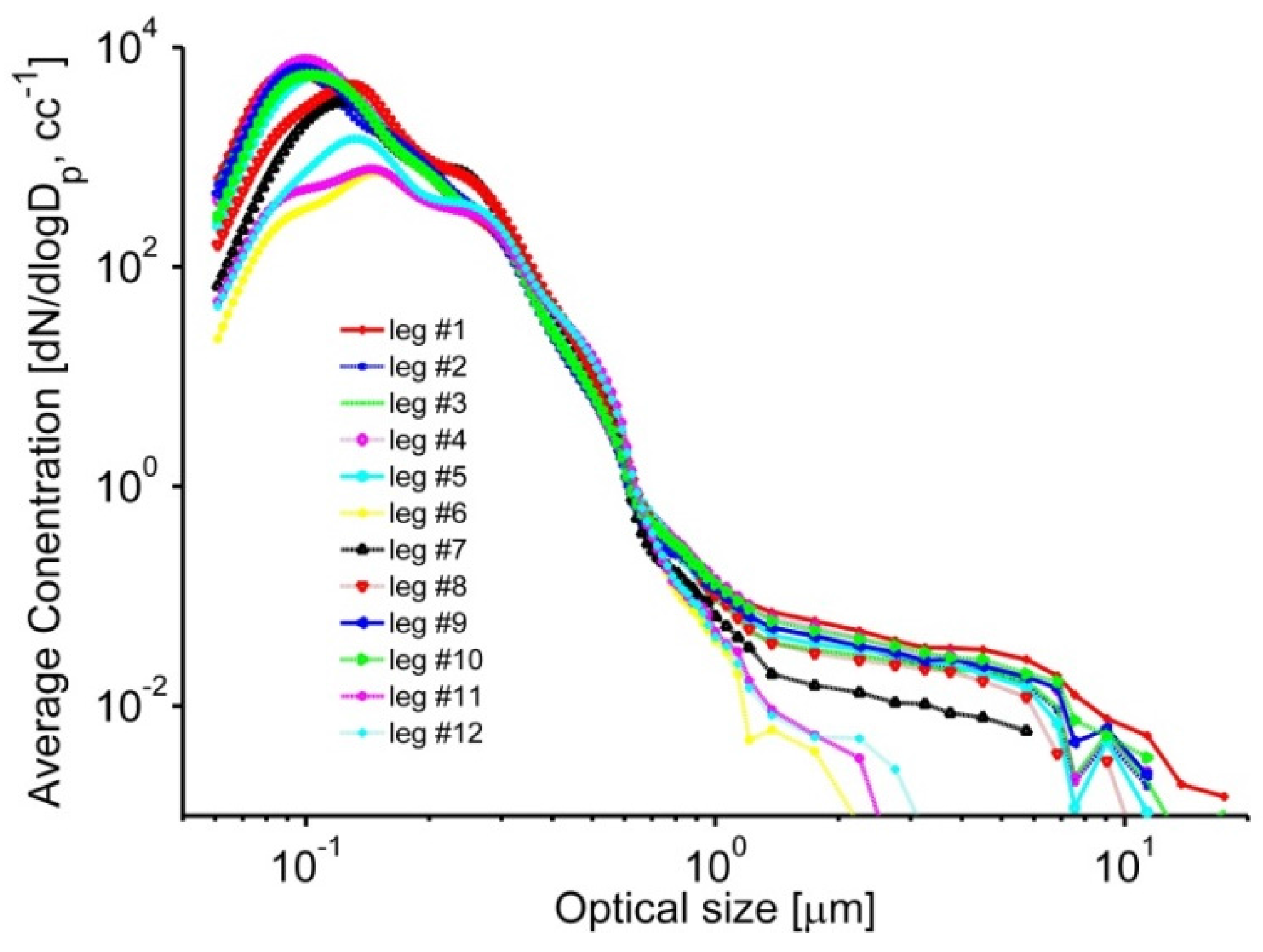
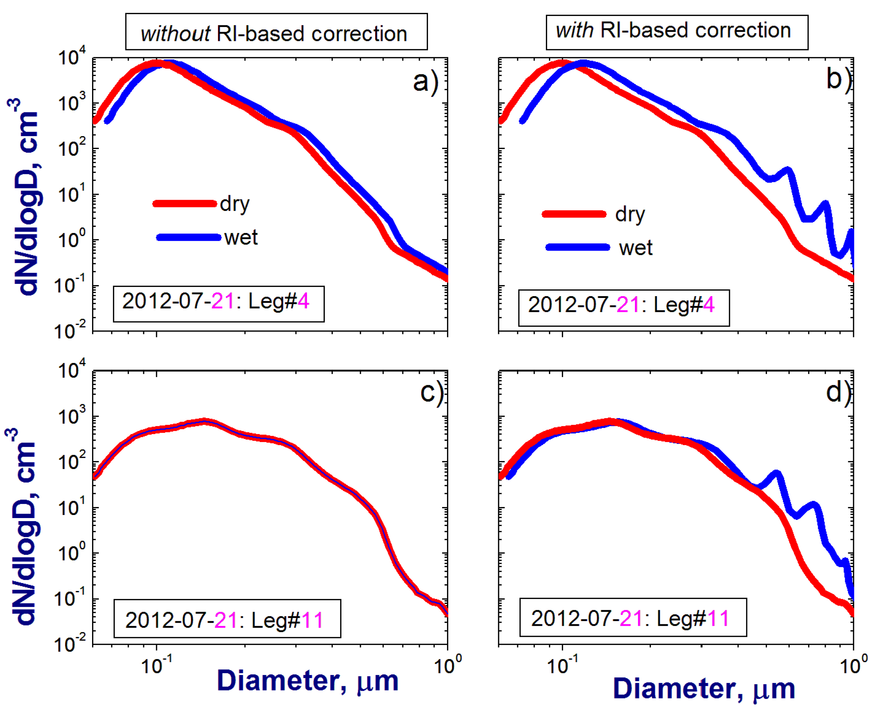
4.3. Size Distribution

4.4. Scattering Coefficient Calculations
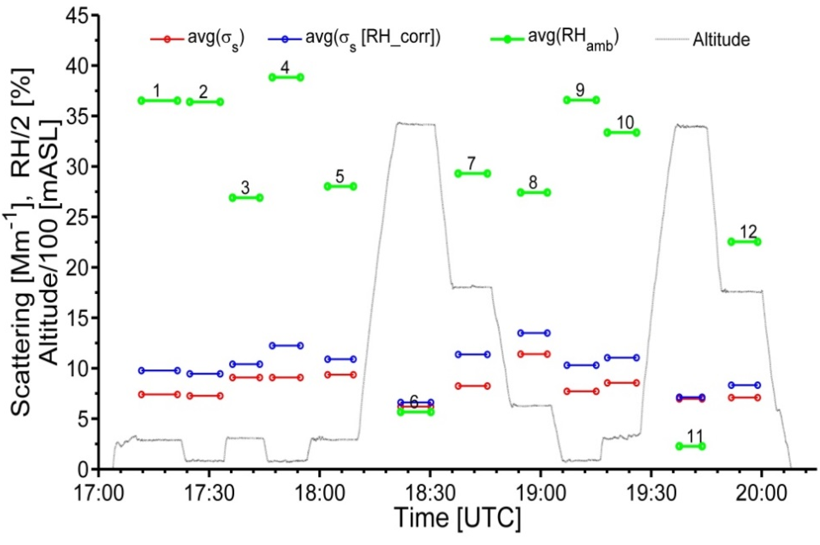
5. Results


| Mean | StDv | RMSE | a | b | |
|---|---|---|---|---|---|
| 0.45 µm | |||||
| σobs | 20.05 | 12.26 | - | - | - |
| σmod,org | 13.70 | 10.42 | 7.49 | −1.58 (0.80) | 0.75 (0.06) |
| σmod,adj | 22.75 | 17.09 | 7.10 | −2.54 (1.33) | 1.24 (0.10) |
| 0.55 µm | |||||
| σobs | 14.85 | 8.98 | - | - | - |
| σmod,org | 8.80 | 6.78 | 6.99 | −1.30 (0.63) | 0.68 (0.06) |
| σmod,adj | 15.89 | 12.17 | 5.01 | −2.25 (1.13) | 1.21 (0.11) |
| 0.70 µm | |||||
| σobs | 8.73 | 5.28 | - | - | - |
| σmod,org | 4.87 | 3.78 | 4.61 | −0.73 (0.45) | 0.64 (0.07) |
| σmod,adj | 9.77 | 7.57 | 3.85 | −1.40 (0.90) | 1.26 (0.15) |
6. Sensitivity Study


| Mean | StDv | RMSE | a | b | |
|---|---|---|---|---|---|
| σobs | 14.85 | 8.98 | - | - | - |
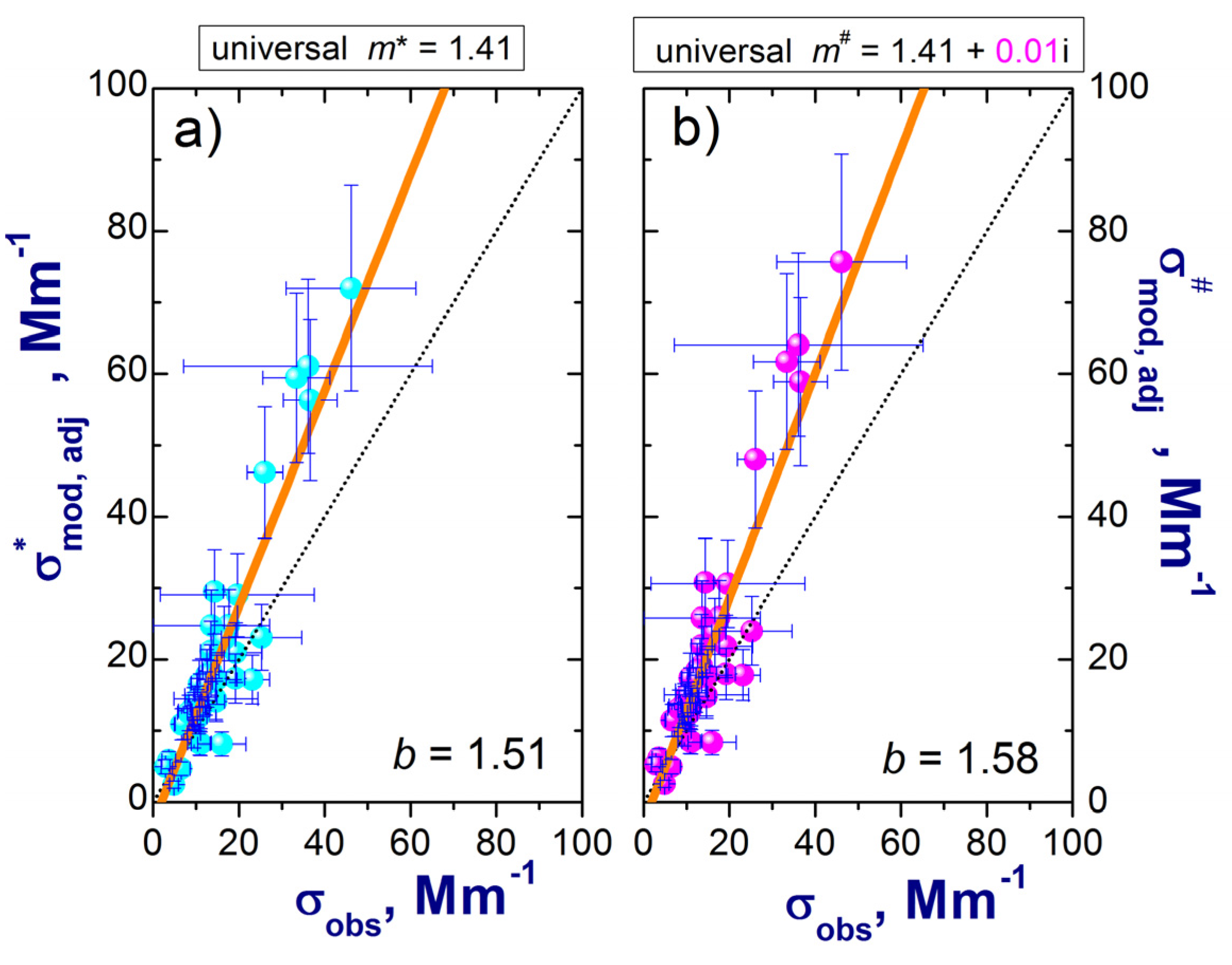
| 19.82 | 15.46 | 9.17 | −2.85 (1.42) | 1.51 (0.14) | |
| 20.67 | 16.19 | 10.20 | −2.96 (1.48) | 1.58 (0.15) |
7. Summary
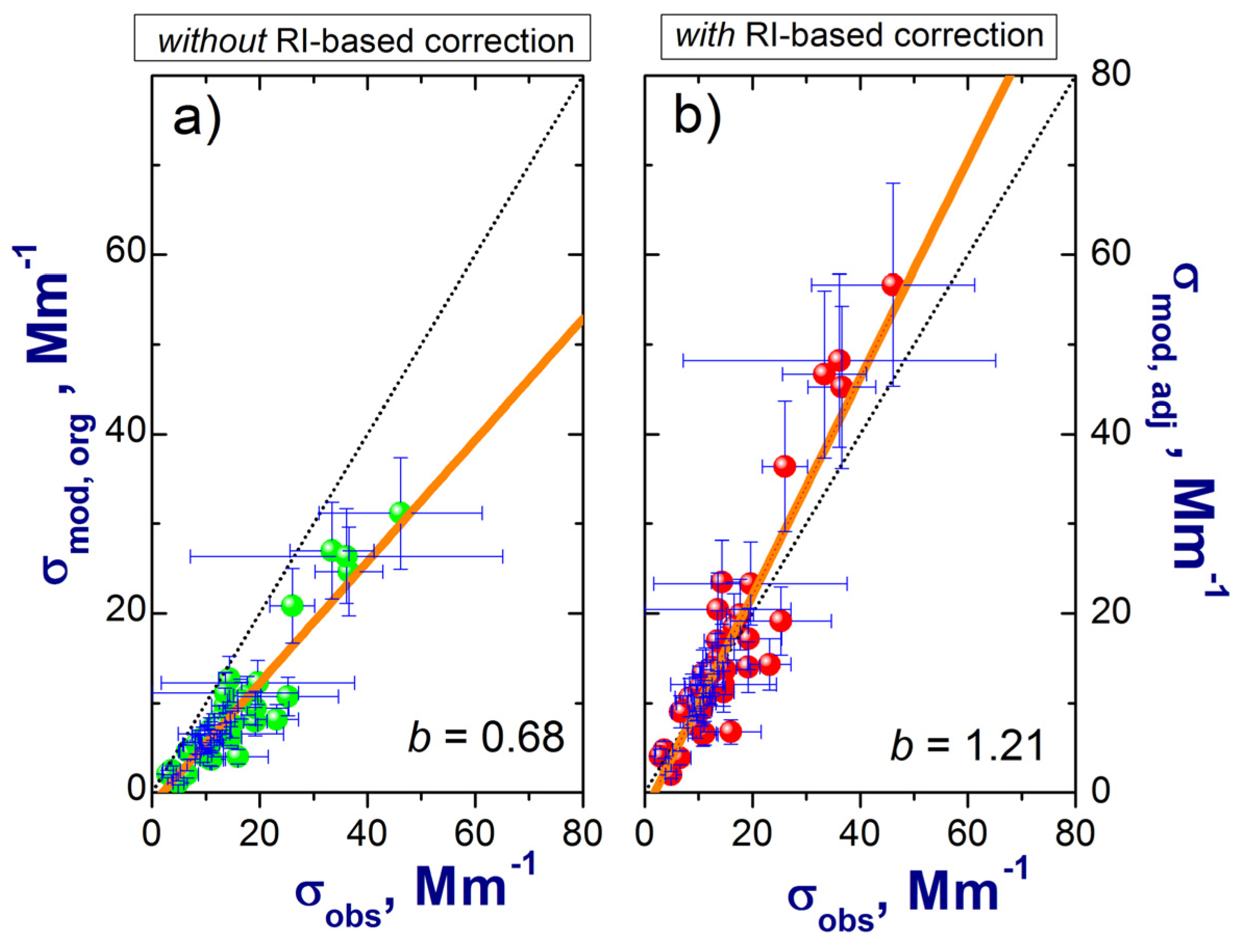
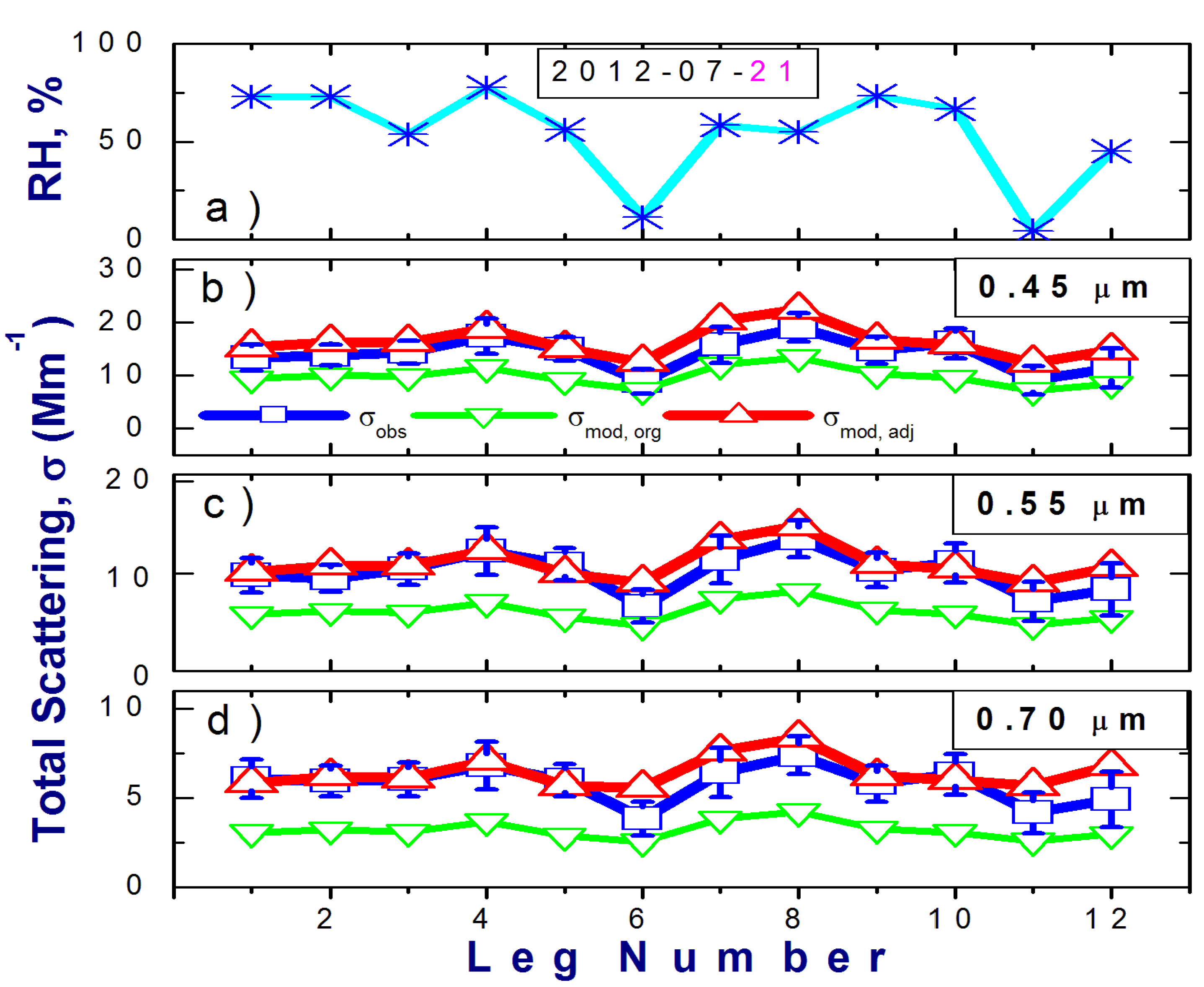
- Analysis based on using the “complete” data set addresses our first question, namely: What level of agreement between the in-flight measured and calculated values of total scattering coefficient can be achieved at ambient RH? We demonstrate that despite the well-known limitations of airborne measurements and the assumptions required by our approach, we can obtain good agreement between the observed and calculated scattering at three wavelengths (about 13% at 0.45 µm, 7% at 0.55 µm, and 12% at 0.7 µm on average) using the RI-based correction for OPC-derived size spectra and the best available chemical composition data for the RI estimation. We calculate the total scattering coefficient from the combined size spectra (UHSAS, PCASP and CAS data) and aerosol composition (AMS and SP2 data) at ambient conditions with a wide range of relative humidity values (from 5% to 80%). These calculations involve several assumptions, such as the homogeneous internal mixture assumption for estimating the hygroscopic growth factor and complex refractive index (RI) at ambient conditions, and simplified specification of particle geometry (homogeneous spheres) for Mie calculations.
- Analysis based on using an “incomplete” dataset addresses our second question, namely: What is the effect of ignoring the influence of chemical composition data on this agreement? We illustrate that ignoring the RI-based correction in the TCAP data can cause a substantial underestimation (about 40% on average) of the ambient calculated scattering when noticeable discrepancies between the actual RIs and those used for the OPC calibration have occurred. Our findings are in harmony with previous studies, which have highlighted the importance of the RI-based correction and have suggested its parameterization for non-absorbing aerosol assuming that the RI-based correction is a function of real RI only [30,31]. In comparison with these important parameterizations, our approach is more flexible in terms of available inputs (complex RI is estimated explicitly from the complementary chemical composition data), and therefore in terms of the expected applications (both non-absorbing and absorbing aerosol sampled by ground-based and airborne instruments).
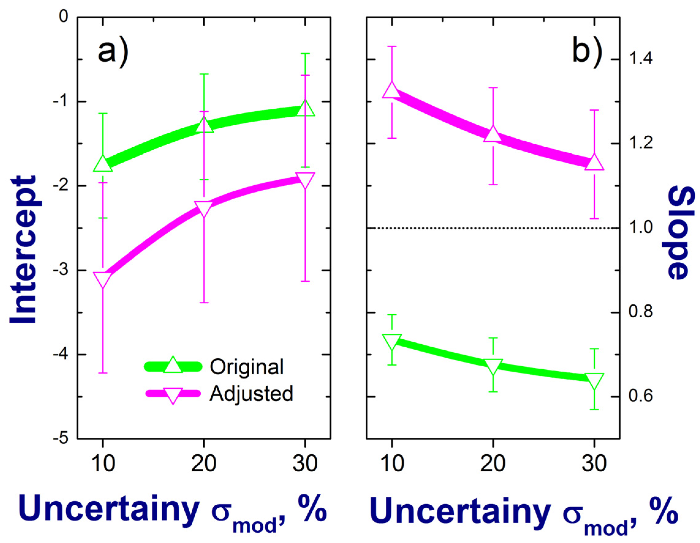
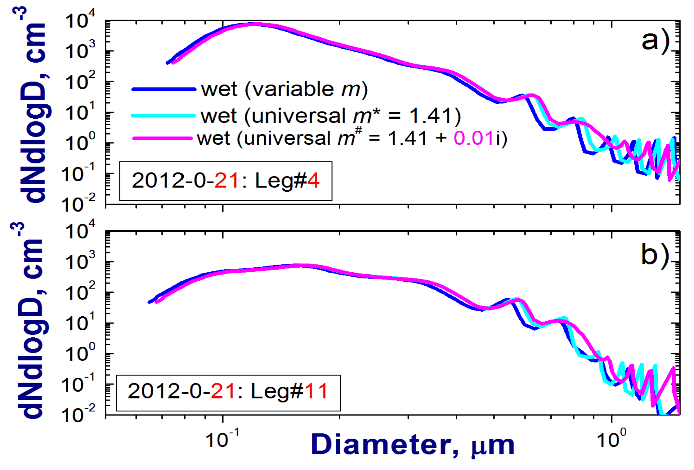
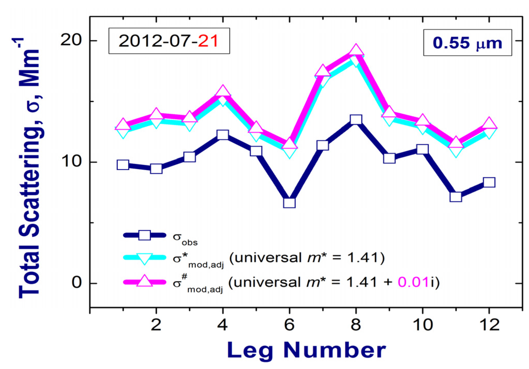
- Analysis based on using an “incomplete” dataset also addresses our third question, namely: How sensitive is this agreement to the assumed RI value, particularly if the assumed RI is non-representative of the ambient aerosol? We illustrate in a sensitivity study that using a non-representative universal RI instead of the actual RI can result in a large overestimation (about 35% on average) of the calculated total scattering at ambient RH, and this overestimation is sensitive to specification of the imaginary part of the complex RI, even for weakly-absorbing aerosol. This sensitivity study suggests that the usefulness of assumptions required for universal RI estimation could be marginal, particularly when applied to the strong temporal and spatial variability of aerosol sampled by research aircraft. As a result, calculations of aerosol optical properties based on these assumptions should be used with caution and other possible approaches should be considered to improve the RI estimation. These possibilities include application of conventional iterative or optimization schemes where a set of assumed representative RI values is used to minimize differences between the measured and calculated aerosol properties of interest [34,40,70].
Acknowledgments
Author Contributions
Conflicts of Interest
Appendix A. Merging of Size Distributions
Appendix B. Contributions from Particles of Different Sizes to Scattering

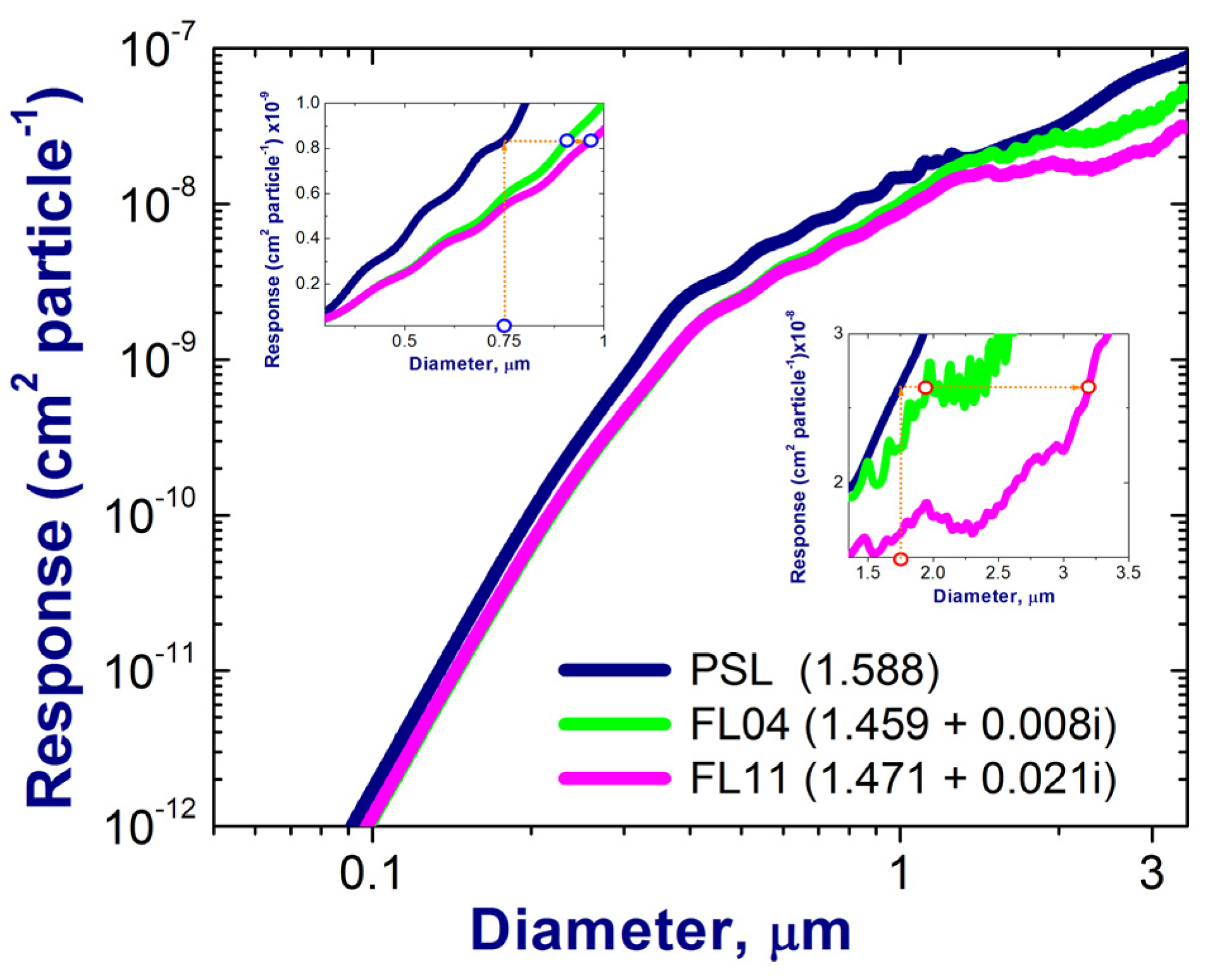
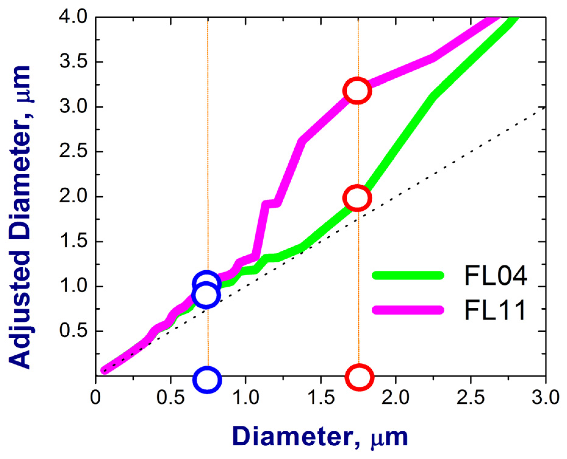
Appendix C. Correction of OPC-derived Size Spectra


References
- Wang, X.; Heald, C.L.; Ridley, D.A.; Schwarz, J.P.; Spackman, J.R.; Perring, A.E.; Coe, H.; Liu, D.; Clarke, A.D. Exploiting simultaneous observational constraints on mass and absorption to estimate the global direct radiative forcing of black carbon and brown carbon. Atmos. Chem. Phys. 2014, 14, 10989–11010. [Google Scholar] [CrossRef]
- Sundström, A.-M.; Arola, A.; Kolmonen, P.; Xue, Y.; de Leeuw, G.; Kulmala, M. On the use of a satellite remote-sensing-based approach for determining aerosol direct radiative effect over land: A case study over China. Atmos. Chem. Phys. 2015, 15, 505–518. [Google Scholar] [CrossRef]
- Adachi, K.; Chung, S.H.; Buseck, P.R. Shapes of soot aerosol particles and implications for their effects on climate. J. Geophys. Res. 2010, 115, D15206. [Google Scholar] [CrossRef]
- Bond, T.C.; Doherty, S.J.; Fahey, D.W.; Forster, P.M.; Berntsen, T.; DeAngelo, B.J.; Flanner, M.G.; Ghan, S.; Kärcher, B.; Koch, D.; et al. Bounding the role of black carbon in the climate system: A scientific assessment. J. Geophys. Res. Atmos. 2013, 118, 5380–5552. [Google Scholar] [CrossRef]
- China, S.; Mazzoleni, C.; Gorkowski, K.; Aiken, A.C.; Dubey, M.K. Morphology and mixing state of individual freshly emitted wildfire carbonaceous particles. Nat. Comm. 2013, 4, 2122. [Google Scholar] [CrossRef] [PubMed]
- Fast, J.D.; Allan, J.; Bahreini, R.; Craven, J.; Emmons, L.; Ferrare, R.; Hayes, P.L.; Hodzic, A.; Holloway, J.; Hostetler, C.; et al. Modeling regional aerosol and aerosol precursor variability over California and its sensitivity to emissions and long-range transport during the 2010 CalNex and CARES campaigns. Atmos. Chem. Phys. 2014, 14, 10013–10060. [Google Scholar] [CrossRef]
- Washenfelder, R.A.; Attwood, A.R.; Brock, C.A.; Guo, H.; Xu, L.; Weber, R.J.; Ng, N.L.; Allen, H.M.; Ayres, B.R.; Baumann, K.; et al. Biomass burning dominates brown carbon absorption in the rural southeastern United States. Geophys. Res. Lett. 2015, 42, 653–664. [Google Scholar] [CrossRef]
- Müller, D.; Hostetler, C.A.; Ferrare, R.A.; Burton, S.P.; Chemyakin, E.; Kolgotin, A.; Hair, J.W.; Cook, A.L.; Harper, D.B.; Rogers, R.R.; et al. Airborne Multiwavelength High Spectral Resolution Lidar (HSRL-2) observations during TCAP 2012: Vertical profiles of optical and microphysical properties of a smoke/urban haze plume over the northeastern coast of the US. Atmos. Meas. Tech. 2014, 7, 3487–3496. [Google Scholar] [CrossRef] [Green Version]
- Russell, P.B.; Kacenelenbogen, M.; Livingston, J.M.; Hasekamp, O.P.; Burton, S.P.; Schuster, G.L.; Johnson, M.S.; Knobelspiesse, K.D.; Redemann, J.; Ramachandran, S.; Holben, B. A multiparameter aerosol classification method and its application to retrievals from spaceborne polarimetry. J. Geophys. Res. Atmos. 2014, 119, 9838–9863. [Google Scholar] [CrossRef]
- Chaikovskaya, L.; Dubovik, O.; Litvinov, P.; Grudo, J.; Lopatsin, A.; Chaikovsky, A.; Denisov, S. Analytical algorithm for modeling polarized solar radiation transfer through the atmosphere for application in processing complex lidar and radiometer measurements. J. Quant. Spectrosc. Radiat. Trans. 2015, 151, 275–286. [Google Scholar] [CrossRef]
- Kokhanovsky, A.A.; Davis, A.B.; Cairns, B.; Dubovik, O.; Hasekamp, O.P.; Sano, I.; Mukai, S.; Rozanov, V.V.; Litvinov, P.; Lapyonok, T.; et al. Space-based remote sensing of atmospheric aerosols: The multi-angle spectro-polarimetric frontier. Earth-Sci. Rev. 2015. [Google Scholar] [CrossRef]
- Baumgardner, D.; Brenguier, J.L.; Bucholtz, A.; Coe, H.; DeMott, P.; Garrett, T.J.; Gayet, J.F.; Hermann, M.; Heymsfield, A.; Korolev, A.; et al. Airborne instruments to measure atmospheric aerosol particles, clouds and radiation: A cook’s tour of mature and emerging technology. Atmos. Res. 2011, 102, 10–29. [Google Scholar] [CrossRef]
- McFarquhar, G.; Schmid, B.; Korolev, A.; Ogren, J.A.; Russell, P.B.; Tomlinson, J.; Turner, D.D.; Wiscombe, W. Airborne instrumentation needs for climate and atmospheric research. Bull. Amer. Meteor. Soc. 2011, 92, 1193–1196. [Google Scholar] [CrossRef]
- Konwar, M.; Panicker, A.S.; Axisa, D.; Prabha, T.V. Near-cloud aerosols in monsoon environment and its impact on radiative forcing. J. Geophys. Res. Atmos. 2015, 120. [Google Scholar] [CrossRef]
- Russell, P.B.; Kinne, S.A.; Bergstrom, R.W. Aerosol climate effects: Local radiative forcing and column closure experiments. J. Geophys. Res. 1997, 102, 9397–9407. [Google Scholar] [CrossRef]
- Schmid, B.; Livingston, J.M.; Russell, P.B.; Durkee, P.A.; Jonsson, H.H.; Collins, D.R.; Flagan, R.C.; Seinfeld, J.H.; Gassó, S.; Hegg, D.A.; et al. Clear-sky closure studies of lower tropospheric aerosol and water vapor during ACE-2 using airborne sunphotometer, airborne in-situ, space-borne, and ground-based measurements. Tellus B 2000, 52, 568–593. [Google Scholar] [CrossRef]
- Malm, W.C.; Day, D.E.; Carrico, C.; Kreidenweis, S.M.; Collett, J.L., Jr.; McMeeking, G.; Lee, T.; Carrillo, J.; Schichtel, B. Intercomparison and closure calculations using measurements of aerosol species and optical properties during the Yosemite Aerosol Characterization Study. J. Geophys. Res. 2005, 110, D14302. [Google Scholar] [CrossRef]
- Mack, L.A.; Levin, E.J.T.; Kreidenweis, S.M.; Obrist, D.; Moosmüller, H.; Lewis, K.A.; Arnott, W.P.; McMeeking, G.R.; Sullivan, A.P.; Wold, C.E.; et al. Optical closure experiments for biomass smoke aerosols. Atmos. Chem. Phys. 2010, 10, 9017–9026. [Google Scholar] [CrossRef] [Green Version]
- Marshall, J.; Lohmann, U.; Leaitch, W.R.; Lehr, P.; Hayden, K. Aerosol scattering as a function of altitude in a coastal environment. J. Geophys. Res. 2007, 112, D14203. [Google Scholar] [CrossRef]
- Ma, N.; Birmili, W.; Müller, T.; Tuch, T.; Cheng, Y.F.; Xu, W.Y.; Zhao, C.S.; Wiedensohler, A. Tropospheric aerosol scattering and absorption over central Europe: A closure study for the dry particle state. Atmos. Chem. Phys. 2014, 14, 6241–6259. [Google Scholar] [CrossRef]
- Zieger, P.; Fierz-Schmidhauser, R.; Poulain, L.; Müller, T.; Birmili, W.; Spindler, G.; Wiedensohler, A.; Baltensperger, U.; Weingartner, E. Influence of water uptake on the aerosol particle light scattering coefficients of the Central European aerosol. Tellus B 2014, 66, 22716. [Google Scholar] [CrossRef]
- Wang, J.; Flagan, R.C.; Seinfeld, J.H.; Jonsson, H.H.; Collins, D.R.; Russell, P.B.; Schmid, B.; Redemann, J.; Livingston, J.M.; Gao, S.; et al. Clear-column radiative closure during ACE-Asia: Comparison of multiwavelength extinction derived from particle size and composition with results from sunphotometry. J. Geophys. Res. 2002, 107, 4688. [Google Scholar] [CrossRef]
- Parworth, C.; Fast, J.; Mei, F.; Shippert, T.; Sivaraman, C.; Tilp, A.; Watson, T.; Zhang, Q. Long-term measurements of submicrometer aerosol chemistry at the Southern Great Plains (SGP) using an Aerosol Chemical Speciation Monitor (ACSM). Atmos. Environ. 2015, 106, 43–55. [Google Scholar] [CrossRef]
- Schmid, B.; Tomlinson, J.M.; Hubbe, J.M.; Comstock, J.M.; Mei, F.; Chand, D.; Pekour, M.S.; Kluzek, C.D.; Andrews, E.; Biraud, S.C.; et al. The DOE ARM Aerial Facility. Bull. Am. Meteor. Soc. 2014, 95, 723–742. [Google Scholar] [CrossRef]
- Kassianov, E.; Flynn, C.; Redemann, J.; Schmid, B.; Russell, P.B.; Sinyuk, A. Initial assessment of the Spectrometer for Sky-Scanning, Sun-Tracking Atmospheric Research (4STAR)-based aerosol retrieval: Sensitivity study. Atmosphere 2012, 3, 495–521. [Google Scholar] [CrossRef]
- Dunagan, S.; Johnson, R.; Zavaleta, J.; Russell, P.; Schmid, B.; Flynn, C.; Redemann, J.; Shinozuka, Y.; Livingston, J.; Segal-Rosenhaimer, M. Spectrometer for Sky-Scanning Sun-Tracking Atmospheric Research (4STAR): Instrument technology. Remote Sens. 2013, 5, 3872–3895. [Google Scholar] [CrossRef]
- Segal-Rosenheimer, M.; Russell, P.B.; Schmid, B.; Redemann, J.; Livingston, J.M.; Flynn, C.J.; Johnson, R.R.; Dunagan, S.E.; Shinozuka, Y.; Herman, J.; et al. Tracking elevated pollution layers with a newly developed hyperspectral Sun/Sky spectrometer (4STAR): Results from the TCAP 2012 and 2013 campaigns. J. Geophys. Res. Atmos. 2014, 119, 2611–2628. [Google Scholar] [CrossRef]
- Allen, G.; Coe, H.; Clarke, A.; Bretherton, C.; Wood, R.; Abel, S.J.; Barrett, P.; Brown, P.; George, R.; Freitag, S.; et al. South East Pacific atmospheric composition and variability sampled along 20° S during VOCALS-Rex. Atmos. Chem. Phys. 2011, 11, 5237–5262. [Google Scholar] [CrossRef]
- Kleinman, L.I.; Daum, P.H.; Lee, Y.-N.; Lewis, E.R.; Sedlacek, A.J., III; Senum, G.I.; Springston, S.R.; Wang, J.; Hubbe, J.; Jayne, J.; et al. Aerosol concentration and size distribution measured below, in, and above cloud from the DOE G-1 during VOCALS-REx. Atmos. Chem. Phys. 2012, 11, 207–223. [Google Scholar] [CrossRef]
- Liu, Y.; Daum, P.H. The effect of refractive index on size distributions and light scattering coefficients derived from optical particle counters. J. Aerosol. Sci. 2000, 31, 945–957. [Google Scholar] [CrossRef]
- Ames, R.B.; Hand, J.L.; Kreidenweis, S.M.; Day, D.E.; Malm, W.C. Optical measurements of aerosol size distributions in Great Smokey Mountains National Park: Dry aerosol characterization. J. Air Waste Manag. Assoc. 2000, 50, 665–676. [Google Scholar] [CrossRef] [PubMed]
- Garvey, D.M.; Pinnick, R.G. Response characteristics of the particle measuring systems active scattering aerosol spectrometer probe (ASASP-X). Aerosol Sci. Technol. 1983, 2, 477–488. [Google Scholar] [CrossRef]
- Kim, Y.J.; Boatman, J.F. Size calibration corrections for the Forward Scattering Spectrometer Probe (FSSP) for measurement of atmospheric aerosols of different refractive indices. J. Atmos. Oceanic Technol. 1990, 7, 681–688. [Google Scholar] [CrossRef]
- Bukowiecki, N.; Zieger, P.; Weingartner, E.; Juranyi, Z.; Gysel, M.; Neininger, B.; Schneider, B.; Hueglin, C.; Ulrich, A.; Wichser, A.; et al. Ground-based and airborne in-situ measurements of the Eyjafjallajökull volcanic aerosol plume in Switzerland in spring 2010. Atmos. Chem. Phys. 2011, 11, 10011–10030. [Google Scholar] [CrossRef] [Green Version]
- Kondo, Y. Effects of black carbon on climate: Advances in measurement and modeling. Monogr. Environ. Earth Planets 2015, 3, 1–85. [Google Scholar] [CrossRef]
- Kreidenweis, S.M.; Asa-Awuku, A. Aerosol Hygroscopicity: Particle water content and its role in atmospheric processes. Treat. Geochem.: Second Ed. 2013, 5, 331–361. [Google Scholar]
- Jensen, T.L.; Kreidenweis, S.M.; Kim, Y.; Sievering, H.; Pszenny, A. Aerosol distributions measured in the North Atlantic marine boundary layer during ASTEX/MAGE. J. Geophys. Res. 1996, 101, 4455–4467. [Google Scholar]
- Swietlicki, E.; Zhou, J.; Berg, O.H.; Martinsson, B.G.; Frank, G.; Cederfelt, S.-I.; Dusek, U.; Berner, A.; Birmili, W.; Wiedensohler, A.; et al. A closure study of sub-micrometer aerosol particle hygroscopic behavior. Atmos. Res. 1999, 50, 205–240. [Google Scholar] [CrossRef]
- Dusek, U.; Frank, G.P.; Massling, A.; Zeromskiene, K.; Iinuma, Y.; Schmid, O.; Helas, G.; Hennig, T.; Wiedensohler, A.; Andreae, M.O. Water uptake by biomass burning aerosol at sub- and supersaturated conditions: Closure studies and implications for the role of organics. Atmos. Chem. Phys. 2011, 11, 9519–9532. [Google Scholar] [CrossRef]
- Kassianov, E.; Barnard, J.; Pekour, M.; Berg, L.K.; Shilling, J.; Flynn, C.; Mei, F.; Jefferson, A. Simultaneous retrieval of effective refractive index and density from size distribution and light-scattering data: Weakly absorbing aerosol. Atmos. Meas. Tech. 2014, 7, 3247–3261. [Google Scholar] [CrossRef]
- Titos, G.; Jefferson, A.; Sheridan, P.J.; Andrews, E.; Lyamani, H.; Alados-Arboledas, L.; Ogren, J.A. Aerosol light-scattering enhancement due to water uptake during the TCAP campaign. Atmos. Chem. Phys. 2014, 14, 7031–7043. [Google Scholar] [CrossRef]
- Collins, D.R.; Flagan, R.C.; Seinfeld, J.H. Improved inversion of scanning DMA data. Aerosol Sci. Technol. 2002, 36, 1–9. [Google Scholar] [CrossRef]
- Schmid, B.; Ferrare, R.; Flynn, C.; Elleman, R.; Covert, D.; Strawa, A.; Welton, E.; Turner, D.; Jonsson, H.; Redemann, J.; et al. How well do state-of-the-art techniques measuring the vertical profile of tropospheric aerosol extinction compare? J. Geophys. Res. 2006, 111, D05S07. [Google Scholar] [CrossRef]
- Zelenyuk, A.; Imre, D.; Wilson, J.; Zhang, Z.; Wang, J.; Mueller, K. Airborne Single Particle Mass Spectrometers (SPLAT II& miniSPLAT) and new software for data visualization and analysis in a geo-spatial context. J. Am. Soc. Mass Spectrom. 2015, 26, 257–270. [Google Scholar] [CrossRef] [PubMed]
- Berg, L.; Fast, J.D.; Barnard, J.C.; Burton, S.P.; Cairns, B.; Chand, D.; Comstock, J.M.; Dunagan, S.; Ferrare, R.A.; Flynn, C.J.; et al. The Two-Column Aerosol Project: Phase I overview and impact of elevated aerosol layers on aerosol optical depth. J. Geophys. Res. Atmos. 2015. under review. [Google Scholar]
- Esteve, A.R.; Highwood, E.J.; Morgan, W.T.; Allen, G.; Coe, H.; Grainger, R.G.; Brown, P.; Szpek, K. A study on the sensitivities of simulated aerosol optical properties to composition and size distribution using airborne measurements. Atmos. Environ. 2014, 89, 517–524. [Google Scholar] [CrossRef]
- Twomey, S. Comparison of constrained linear inversion and an iterative nonlinear algorithm applied to indirect estimation of particle-size distributions. J. Comput. Phys. 1975, 18, 188–200. [Google Scholar] [CrossRef]
- Markowski, G.R. Improving Twomey’s Algorithm for Inversion of Aerosol Measurement Data. Aerosol Sci. Technol. 1987, 7, 127–141. [Google Scholar] [CrossRef]
- Moteki, N.; Kondo, Y. Effects of mixing state on black carbon measurements by laser-induced incandescence. Aerosol Sci. Technol. 2007, 41, 398–417. [Google Scholar] [CrossRef]
- Sedlacek, A.J., III; Lewis, E.R.; Kleinman, L.; Xu, J.; Zhang, Q. Determination of and evidence for non-core-shell structure of particles containing black carbon using the Single-Particle Soot Photometer (SP2). Geophys. Res. Lett. 2012, 39. [Google Scholar] [CrossRef]
- Pekour, M.S.; Schmid, B.; Chand, D.; Hubbe, J.M.; Kluzek, C.D.; Nelson, D.A.; Tomlinson, J.M.; Cziczo, D.J. Development of a new airborne humidigraph system. Aerosol Sci. Technol. 2013, 47, 201–207. [Google Scholar] [CrossRef]
- Shinozuka, Y.; Johnson, R.R.; Flynn, C.J.; Russell, P.B.; Schmid, B.; Redemann, J.; Dunagan, S.E.; Kluzek, C.D.; Hubbe, J.M.; Segal-Rosenheimer, M.; et al. Hyperspectral aerosol optical depths from TCAP flights. J. Geophys. Res. Atmos. 2013, 118, 12180–12194. [Google Scholar] [CrossRef]
- Anderson, T.L.; Ogren, J.A. Determining aerosol radiative properties using the TSI 3563 Integrating Nephelometer. Aerosol Sci. Technol. 1998, 29, 57–69. [Google Scholar] [CrossRef]
- Hallar, A.G.; Strawa, A.W.; Schmid, B.; Andrews, E.; Ogren, J.; Sheridan, P.; Ferrare, R.; Covert, D.; Elleman, R.; Jonsson, H.; et al. Atmospheric Radiation Measurements Aerosol Intensive Operating Period: Comparison of aerosol scattering during coordinated flights. J. Geophys. Res. 2006, 111, D05S09. [Google Scholar] [CrossRef]
- Barnard, J.C.; Fast, J.D.; Paredes-Miranda, G.; Arnott, W.P.; Laskin, A. Technical note: Evaluation of the WRF-Chem “Aerosol chemical to aerosol optical properties” module using data from the MILAGRO campaign. Atmos. Chem. Phys. 2010, 10, 7325–7340. [Google Scholar] [CrossRef]
- Hu, D.; Chen, J.; Ye, X.; Li, L.; Yang, X. Hygroscopicity and evaporation of ammonium chloride and ammonium nitrate: Relative humidity and size effects on the growth factor. Atmos. Environ. 2011, 45, 2349–2355. [Google Scholar] [CrossRef]
- Healy, R.M.; Evans, G.J.; Murphy, M.; Jurányi, Z.; Tritscher, T.; Laborde, M.; Weingartner, E.; Gysel, M.; Poulain, L.; Kamilli, K.A.; et al. Predicting hygroscopic growth using single particle chemical composition estimates. J. Geophys. Res. Atmos. 2014, 119, 9567–9577. [Google Scholar] [CrossRef]
- Pilinis, C.; Charalampidis, P.E.; Mihalopoulos, N.; Pandis, S.N. Contribution of particulate water to the measured aerosol optical properties of aged aerosol. Atmos. Environ. 2014, 82, 144–153. [Google Scholar] [CrossRef]
- Dubovik, O.; Holben, B.; Eck, T.F.; Smirnov, A.; Kaufman, Y.J.; King, M.D.; Tanré, D.; Slutsker, I. Variability of absorption and optical properties of key aerosol types observed in worldwide locations. J. Atmos. Sci. 2002, 59, 590–608. [Google Scholar] [CrossRef]
- Kokhanovsky, A.A. Aerosol Optics: Light Absorption and Scattering by Particles in the Atmosphere; Springer-Berlin: Heidelberg, Germany, 2008; p. 148. [Google Scholar]
- Barber, P.W.; Hill, S.C. Light Scattering by Particles: Computational Methods; World Scientific Publishing: Singapore, 1990. [Google Scholar]
- Scarnato, B.V.; Vahidinia, S.; Richard, D.T.; Kirchstetter, T.W. Effects of internal mixing and aggregate morphology on optical properties of black carbon using a discrete dipole approximation model. Atmos. Chem. Phys. 2013, 13, 5089–5101. [Google Scholar] [CrossRef]
- Lesins, G.; Chylek, P.; Lohmann, U. A study of internal and external mixing scenarios and its effect on aerosol optical properties and direct radiative forcing. J. Geophys. Res. Atmos. 2002, 107, 4094–4106. [Google Scholar] [CrossRef]
- Freney, E.J.; Adachi, K.; Buseck, P.R. Internally mixed atmospheric aerosol particles: Hygroscopic growth and light scattering. J. Geophys. Res. Atmos. 2010, 115, D19210. [Google Scholar] [CrossRef]
- Wex, H.; Neususs, C.; Wendisch, M.; Stratmann, F.; Koziar, C.; Keil, A.; Wiedensohler, A.; Ebert, M. Particle scattering, backscattering, and absorption coefficients: An in situ closure and sensitivity study. J. Geophys. Res. Atmos. 2012, 107, 8122. [Google Scholar] [CrossRef]
- York, D.; Evensen, N.M.; Lopez Martinez, M.; de Basabe Delgado, J. Unified equations for the slope, intercept, and standard errors of the best straight line. Am. J. Phys. 2004, 72, 367–375. [Google Scholar] [CrossRef]
- Petäjä, T.; Mauldin, R.L., III; Kosciuch, E.; McGrath, J.; Nieminen, T.; Paasonen, P.; Boy, M.; Adamov, A.; Kotiaho, T.; Kulmala, M. Sulfuric acid and OH concentrations in a boreal forest site. Atmos. Chem. Phys. 2009, 9, 7435–7448. [Google Scholar] [CrossRef]
- Zieger, P.; Weingartner, E.; Henzing, J.; Moerman, M.; de Leeuw, G.; Mikkilä, J.; Ehn, M.; Petäjä, T.; Clémer, K.; van Roozendael, M.; et al. Comparison of ambient aerosol extinction coefficients obtained from in-situ, MAX-DOAS and LIDAR measurements at Cabauw. Atmos. Chem. Phys. 2011, 11, 2603–2624. [Google Scholar] [CrossRef]
- Cantrell, C.A. Technical Note: Review of methods for linear least-squares fitting of data and application to atmospheric chemistry problems. Atmos. Chem. Phys. 2008, 8, 5477–5487. [Google Scholar] [CrossRef]
- Hand, J.L.; Kreidenweis, S.M. A new method for retrieving particle refractive index and effective density from aerosol size distribution data. Aerosol Sci. Tech. 2002, 36, 1012–1026. [Google Scholar] [CrossRef]
- McComiskey, A.; Feingold, G.; Frisch, A.S.; Turner, D.D.; Miller, M.A.; Chiu, J.C.; Min, Q.; Ogren, J.A. An assessment of aerosol-cloud interactions in marine stratus clouds based on surface remote sensing. J. Geophys. Res. 2009, 114, D09203. [Google Scholar] [CrossRef]
- Modini, R.L.; Frossard, A.A.; Ahlm, L.; Russell, L.M.; Corrigan, C.E.; Roberts, G.C.; Hawkins, L.N.; Schroder, J.C.; Bertram, A.K.; Zhao, R.; et al. Primary marine aerosol-cloud interactions off the coast of California. J. Geophys. Res. Atmos. 2015, 120. [Google Scholar] [CrossRef]
- Yu, H.; Chin, M.; Bian, H.; Yuan, T.; Prospero, J.M.; Omar, A.H.; Remer, L.A.; Winker, D.M.; Yang, Y.; Zhang, Y.; Zhang, Z.; et al. Quantification of trans-Atlantic dust transport from seven-year (2007–2013) record of CALIPSO lidar measurements. Remote Sens. Environ. 2015, 159, 232–249. [Google Scholar] [CrossRef]
- Barnard, J.C.; Harrison, L.C. Monotonic responses from monochromatic optical particle counters. Appl. Opt. 1988, 3, 584–592. [Google Scholar] [CrossRef]
- Kennedy, W.J.; Gentle, J.E. Statistical Computing; Marcel Dekker: New York, NY, USA, 1980. [Google Scholar]
© 2015 by the authors; licensee MDPI, Basel, Switzerland. This article is an open access article distributed under the terms and conditions of the Creative Commons Attribution license (http://creativecommons.org/licenses/by/4.0/).
Share and Cite
Kassianov, E.; Berg, L.K.; Pekour, M.; Barnard, J.; Chand, D.; Flynn, C.; Ovchinnikov, M.; Sedlacek, A.; Schmid, B.; Shilling, J.; et al. Airborne Aerosol in Situ Measurements during TCAP: A Closure Study of Total Scattering. Atmosphere 2015, 6, 1069-1101. https://doi.org/10.3390/atmos6081069
Kassianov E, Berg LK, Pekour M, Barnard J, Chand D, Flynn C, Ovchinnikov M, Sedlacek A, Schmid B, Shilling J, et al. Airborne Aerosol in Situ Measurements during TCAP: A Closure Study of Total Scattering. Atmosphere. 2015; 6(8):1069-1101. https://doi.org/10.3390/atmos6081069
Chicago/Turabian StyleKassianov, Evgueni, Larry K. Berg, Mikhail Pekour, James Barnard, Duli Chand, Connor Flynn, Mikhail Ovchinnikov, Arthur Sedlacek, Beat Schmid, John Shilling, and et al. 2015. "Airborne Aerosol in Situ Measurements during TCAP: A Closure Study of Total Scattering" Atmosphere 6, no. 8: 1069-1101. https://doi.org/10.3390/atmos6081069