Applications of Cell-Ratio Constant False-Alarm Rate Method in Coherent Doppler Wind Lidar

Abstract

A cell-ratio constant false-alarm rate (CR-CFAR) method for detecting the Doppler frequency shift is proposed to improve the accuracy of velocity measured by coherent Doppler wind lidar (CWL) in low signal-to-noise ratio (SNR) environments. The method analyzes the spectrum to solve issues of weak signal submergence in noise encountered in the widely used periodogram method. This characteristic is that the signal region slope is larger than the noise region slope in the frequency spectrum. We combined the ratio and CFAR to propose the CR-CFAR method. The peak area is discriminated from the spectrum using this method. By removing background noise, the peak signal is obtained along with the Doppler shift. To verify the CR-CFAR method, a campaign experiment using both CWL and a commercial Doppler lidar was performed in Hami, China (42°32′ N, 94°03′ E) during 1–7 June 2016. The results showed that the proposed method significantly improved the reliability of CWL data under low SNR conditions. The height—at which both horizontal wind speed correlativity and horizontal wind direction correlativity exceeded 0.99—increased by 65 m. The relative deviation of the horizontal wind speed at 120 m decreased from 40.37% to 11.04%. We used the CR-CFAR method to analyze continuous data. A greater number of wind field characteristics were obtained during observation compared to those obtained using the common wind field inversion method.

1. Introduction

The wind field is the direct consequence of wind energy resources. Wind field resource assessment is critical for optimizing wind turbine parameters. Currently, wind field evaluations are predominantly based on wind tower data. Measurement from the wind tower is relatively accurate and has been recognized as an industry standard. However, wind towers require considerable labor and material resources for regular maintenance. If wind resources near a wind turbine are individually assessed by a wind tower in a wind plant, long test cycles and low testing efficiencies are unavoidable [1,2,3]. The double-edge technique for Doppler lidar has favorable application prospects in the wind field [4]. Comparing with direct detection Doppler lidar, CWL or upconversion Doppler lidar has its own advantages in stability [5,6]. CWL likewise has satisfactory application potential on account of its high accuracy compared to the wind cup anemometer; moreover, it can easily obtain two-dimensional or three-dimensional wind field information.

Significant progress on all-fiber coherent Doppler lidar has been made in recent years [7]. In 2007, Kameyama et al. developed an all-fiber coherent Doppler lidar in which the pulse width at a wavelength of 1.5 μm is variable and the range resolution is 150 m [8]. In 2009, LEOSPHERE developed a commercial wind lidar that can determine the wind field in near real time [9,10]. A continuous laser is used in the lidar, and the detection range and resolution are 200 m and 7 m, respectively.

In principle, a pulse laser is preferred for detecting the wind field. In previous work, the present authors focused on developing CWL using pulse laser to industrialize it. Meanwhile, an all-fiber coherent Doppler wind lidar was proposed by Diao et al. in 2014 with a measurement range of 3 km and 0.2 m/s accuracy [11]. In addition, Bu et al. presented campaign observation using a proposed CWL and sounding balloon in 2015. The measurement results from CWL were compared with sounding- and pilot-balloon measurements. The stability and reliability of that CWL were proven [12].

The emitted light of the CWL interacts with atmospheric aerosol particles and the echo signals received by the telescope carrying the Doppler frequency shift. The wind information is thereby obtained. Doppler frequency shift discrimination is the most important step in data processing of CWL lidars because inversion of wind data relies on the Doppler frequency shift. Currently, several Doppler frequency extraction algorithms are widely used in CWL systems. These algorithms include the complete synchronization digital frequency meter, Burg algorithm for the autoregressive (AR) model, modified covariance method for the AR model, fast Fourier transform (FFT), FFT and center of gravity (COG) method, and spectrum zoom with spectrum correction [13].

FFT is also called the periodogram maximum (PM). Estimation of the Doppler shift under a high SNR condition using this method is unbiased. For a certain SNR, the frequency correction accuracy obtained is high owing to the combination of FFT and COG. It is widely used on account of its accuracy and convenient calculations. The disadvantage of FFT is that the correction accuracy is easily affected by the SNR level, and the calibration precision is poor under low SNR conditions. Hence, the estimation of the Doppler shift is biased in the above case [14].

A complete synchronization digital frequency meter can effectively eliminate technical errors of +1. It can be simultaneously used for full-band measurements. However, it is sensitive to noise and cannot be used for measurements at a low SNR [15]. Methods for the AR model have high frequency resolution; nonetheless, the estimation quality is affected by the model order [16,17]. Spectrum zoom with spectrum correction can effectively reduce the error in signal processing; however, the complex algorithm makes the method unsuitable for online wind information inversion [18].

In this paper, a cell-ratio constant false-alarm rate (CR-CFAR) method based on the FFT method is proposed to solve the corruption of weak signals by noise. Results showed that CR-CFAR can assist in accurately filtering the small signal peak to improve the detection accuracy of CWL at a low SNR. The calculations in the algorithm are not large; moreover, CR-CFAR meets the needs of the presently proposed CWL.

2. System and Method

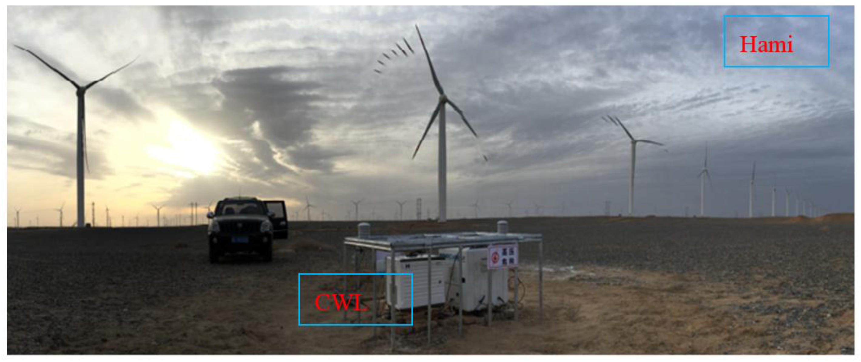
2.1. Proposed CWL System

In general, the maximum detection range required by a wind farm in the vertical direction is less than 300 m because the wind turbine height is normally less than 100 m. Considering wind field detection requirements, we developed a 50-m blind-area coherent Doppler wind lidar with an adjustable height ranging from 50 m to 290 m. The system structure of this lidar is shown in Figure 1. It consists of three parts: the optical transceiver system, heterodyne detection unit, and signal sampling and processing system. The CWL uses a laser with a master oscillator power amplifier (MOPA) and seed injection technique to obtain a 1.54-μm 10-kHz pulse laser.

We compressed the laser pulse width to 200 ns and utilized an output pulse energy of 10 μJ to minimize the blind area. The light emitted by the seed laser was divided into two parts: a local oscillator light and an outgoing light. The frequency of the outgoing light was changed to 120 MHz by an acousto-optic modulator (AOM). The outgoing light entered circulator 1 after multi-stage amplification. Then, by means of circulator 2, it entered the telescope with a diameter of 75 mm. The Doppler frequency shift caused by light-sight wind speed was superimposed on the echo signal light. After mixing the local oscillator signal and echo signal from circulator 3, the heterodyne signal was detected by using the balanced detector.

Electrical amplification and analog-to-digital conversion (ADC) were employed before the Fourier transform to obtain the power spectrum. In principle, the line of sight speed was directly obtained from the power spectrum. A wedge-scanning mirror was used to direct the laser in different directions. After wind speed measurements in different lines of sight, the wind field information was obtained. The main parameters of the CWL are shown in

Table 1. Main technical parameters of the CWL.

Parameter	CWL
Wavelength	1.540 μm
Pulse Repletion Frequency	10 kHz
Intermediate Frequency	120 MHz
Sampling Rate	400 MS/s
Scanning Bearing Number	8
Range Resolution	15 m (typically)
Zenith Angle	28°

.

2.2. Signal and Processing Method

The proposed coherent Doppler wind lidar operates in velocity azimuth display (VAD) mode [19]. The fixed zenith angle is set as $\phi$, where $\phi$ is 28°. Conical scanning of eight symmetric directions can provide more accurate wind information. The velocity detected in each direction is called the line of sight velocity ($V_{LOS}$). The specific CWL data flow processes are outlined as follows:

• Data packets after 2048-point FFT are downloaded from a data acquisition card.
• To obtain the power spectrum, data fetching, format conversion, power descent, etc. are then completed by the host computer.
• Last, the Doppler frequency shift in the line of sight at different heights is estimated by combining the reduced noise, maximum method, and COG.

The relationship between the Doppler frequency shift and line of sight wind speed can be expressed by the following formula [20]:

$$V_{Doppler}=\frac{2}{\lambda }*V_{LOS}$$

(1)

where $V_{Doppler}$ represents the Doppler frequency shift in the line of sight, and $\lambda$ is the wavelength. Finally, according to the characteristics of the velocity azimuth display method (VAD), the real wind field is calculated using the Levenberg–Marquardt method [21,22,23]. Thus, it is evident that the frequency shift detection is the foundation of CWL and the accuracy of wind field detection is directly affected by the detection accuracy of the frequency shift.

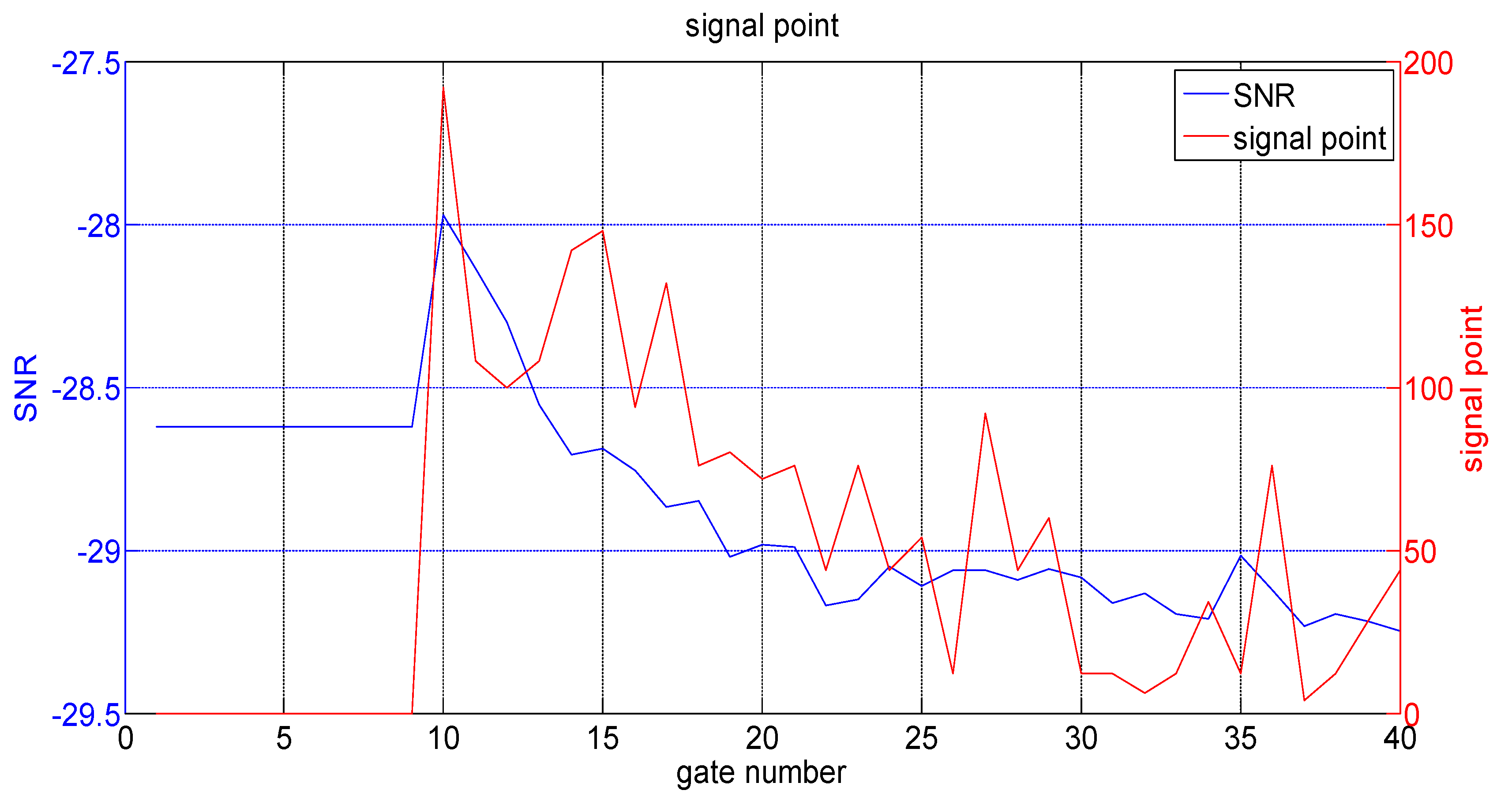
2.3. Doppler Frequency Shift Detection Method

The maximum method is defined as the determination of the maximum value in the power spectrum detected frequency band. The 25-MHz region near the center frequency was chosen as the detected frequency band in the proposed system. However, there can be more than one maximum value in the band on account of signal instability. Some points near the real maximum value cause interference owing to the frequency resolution, amplifier limitations, and some other system errors. This will eventually lead to the conclusion that the maximum method cannot meet the high precision requirements.

Figure 2 shows the power spectrum at 85 m at 03:00 on 21 May 2016. From the power spectrum in the figure, it is clear that the maximum value cannot be correctly highlighted. In COG, the energy center of some points near the peak value is used instead of the maximum value. The signal range used in COG is 1.5 MHz near the center frequency of the proposed system. According to Equation (2), both the Doppler frequency shift and $V_{LOS}$ can be calculated from the COG value.

$$V_{GLOS}=\frac{2}{\lambda }*\left[\frac{F_s}{N}*\left(M_0+\frac{{\displaystyle \sum _{i=x-P_1}^{x+P_2}i*A_i}}{{\displaystyle \sum _{i=x-P_1}^{x+P_2}{A}_i}}-2\right)-f_{AOM}\right]$$

(2)

$V_{GLOS}$ is the line of sight velocity from COG, $\lambda$ represents the wavelength, $F_s$ is the sampling rate, and $N$ denotes the number of sampling points. The maximum value corresponding to the number of power points is denoted as $x$. $P_1$ represents the points on the left side by filtering 1.5 MHz near point $x$, and $P_2$ is the corresponding right part. In addition, $A_i$ is the ith intensity in the FFT power spectrum. The fixed compensation of the point position is $M_0$ and $f_{AOM}$ is the modulated medium frequency.

3. CR-CFAR Method

3.1. Existing Method Limitations in Low SNR Environment

Using COG to estimate the Doppler shift is certainly an unbiased estimation method in high SNR situations [24]. However, when SNR is very low, the estimation becomes biased. In Figure 3, the power spectrum is obtained, for example, at 03:00 on 21 May 2016. According to the meteorological record, the weather is clear and windy. The local wind field in this condition should be continuous and smooth according to the meteorological measurement. The curve in Figure 3a represents the SNR variation with different range gates [25,26].

Compared with the local existing commercial wind lidar, the proposed CWL shows a nonlinear relationship between the measuring height and number of gates, as shown in

Table 2. Relationship between the gate and height.

Gate	Height
10	40 m
11	50 m
13	70 m
15	85 m
16	100 m
18	120 m
20	150 m
22	180 m

. It is obvious from Figure 3a that the SNR at the 15th range gate (−28.56 dB) is higher than the ones at the 20th range gate (−28.69 dB) and 22nd range gate (−28.95 dB). Figure 3b shows that, when the SNR is high, the Doppler frequency shift estimation is unbiased. The 960 spectral points on the horizontal coordinate correspond to the actual 200-MHz bandwidth. The first peak after 120 MHz is easily discriminated because the signal peak is intense, whereas the other nearby peaks are relatively small. Hence, the Doppler frequency shift using COG is precise in this situation. The SNR in Figure 3d has the same level as that in Figure 3c. The first peak after 120 MHz is slightly higher than the first peak before 120 MHz.

In Figure 3c, the first peak after 120 MHz can be separated from the detection area using COG. In Figure 3d, the first peak before 120 MHz will be selected if COG is used because it is larger. In this case, the difference between the selected peak position and the real one is approximately 20 MHz. The difference between $V_{GLOS}$ and $V_{LOS}$ is 15.625 m/s according to Equation (1). In the case of low SNR, the wind speed from COG is incorrect because random errors in the detecting process will adversely affect wind signals when the SNR is low.

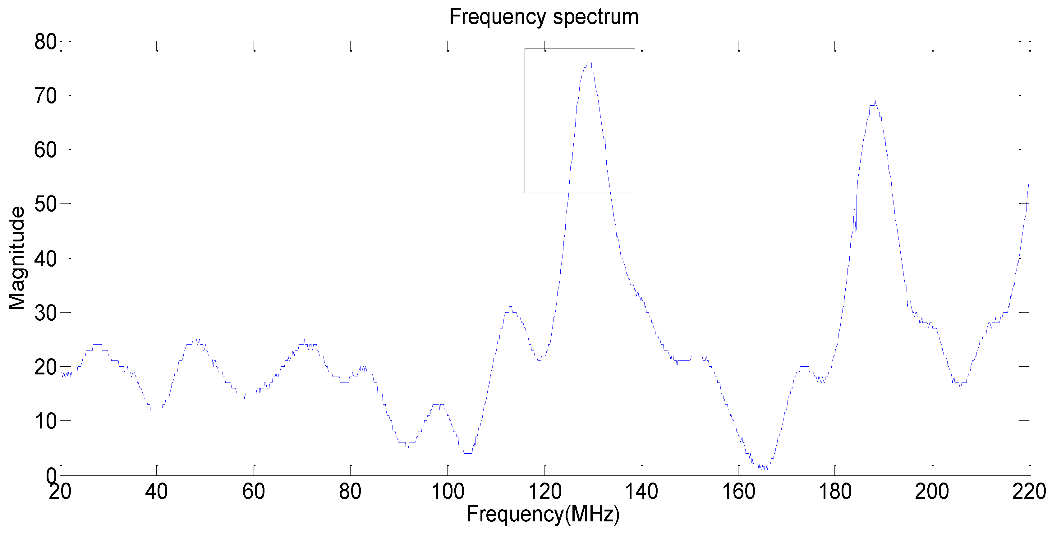
3.2. CR-CFAR for Spectral Analysis

The pulse signal detection method typically includes a binary hypothesis test model, and the observed result has either signal $H_1$ or noise $H_0$ [27]. According to the Neyman–Pearson criterion, a maximum detection probability is usually assumed. Thus, the false alarm probability can be maintained at a certain value [28].

As with a cell-average constant false-alarm rate (CA-CFAR) in the frequency detection [29], the proposed CR-CFAR was designed according to the characteristic of the signal peak in the frequency domain. This characteristic is that the signal region slope is larger than the noise region slope in the frequency spectrum. The ratio can be expressed by the absolute value of the difference of the adjacent data in the frequency spectrum because of the certain frequency interval. Usually, the lidar noise can be regarded as Gaussian white noise after the limit of the band [30]. The squares of the absolute values after FFT are subjected to exponential distribution [27]. Moreover, the absolute values of the difference of the adjacent data are subjected to exponential distribution. Thus, 1000 Monte Carlo experiments were conducted with 99% confidence, and 991 time values were subjected to exponential distribution. The probability distribution function can be expressed as follows [31]:

$$F(x)=1-{{\displaystyle e}}^{-\frac{x}{\eta }},x\ge 0$$

(3)

where $\eta$ is the average power of the background noise.

$${{\displaystyle P}}_{fa}=1-F(x)={{\displaystyle e}}^{-\frac{x}{\eta }}$$

(4)

If ${{\displaystyle P}}_{fa}$ is a constant false alarm probability, ${{\displaystyle P}}_{fa}$ can be given by Equation (4). Taking x = T into Equation (4), the equation can be given as:

$$T=-\eta ·In({{\displaystyle P}}_{fa})$$

(5)

where $T$ is the noise threshold coefficient.

The statistical characteristics of the background noise can be estimated using the ratio of the adjacent cells. The CR-CFAR model is shown in Figure 4. Input signal $x_i$ is sent to a delay line consisting of (L + 1) cells. |d_D| is the unit to be detected. The L − 1 units on the left side of |d_D| are reference units. Summation of all |d_i| values is in the reference cell. We obtain the background estimated mean $\widehat{u}$ of the detection unit after the sum is divided by L − 1. The detection threshold can be described as $U_0=T*\widehat{u}$. The detection threshold in the frequency domain can be described as:

$$\{\begin{array}{c}{H}_1,U_D\ge U_0\\ H_0,U_D<U_0\end{array}$$

(6)

where $\widehat{u}$ is the estimated background noise, and $T$ represents the threshold weighted coefficient. The calculation formula is described as:

$$\widehat{u}=\frac{1}{L-1}{\displaystyle \sum _{i=2}^L|d_i|}$$

(7)

where $L$ is the reference window. In this paper, 50 is used as the reference window. The threshold-weighted coefficient, $T$, is from Equation (5), and ${{\displaystyle P}}_{fa}$ is 0.3 in this system [32].

The specific CR-CFAR method process is outlined below:

• Read the spectrum points and corresponding frequency $x_i$ from the sampling system.
• Estimate background noise $\widehat{u}$ according to the reference window that has been set.
• Calculate the threshold using the threshold-weighted coefficient.
• Compare $U_D$ with $U_0$ to detect whether the current frequency contains the peak signal.
• The range between the two ends of the signal is defined as the peak area.
• The maximum method or COG is applied to the peak area to determine the peak of the Doppler frequency shift.

We used 1000 detection data items, respectively, with CR-CFAR and the widely used CA-CFAR. Figure 5 shows the statistical probability detection with the change of SNR. If a 90% detection probability is used as the system performance evaluation criterion, the minimum detection SNR (−33.3 dB) using CR-CFAR is less than the minimum detection SNR (−32 dB) using CA-CFAR, as shown in Figure 5.

Eight lines of sight exist in CWL. In one scanning period, the unadjacent four directions of the eight are selected in this paper to show the advantage; specifically, directions 2, 4, 6 and 8, as shown in Figure 6. The red curve indicates the line of sight wind speed after CR-CFAR (the new method), and the blue curve is that after COG (the former method). The lidar detection area can be divided into a high SNR area that is from tenth to eighteenth gates (more than approximately −29 dB) and a low SNR area that is gates after 19th one (less than approximately −29 dB). The line of sight velocity after COG is basically similar to the line of sight velocity after CR-CFAR from tenth to eighteenth gates, which is shown in the four parts of Figure 6. However, some line of sight velocity values from CR-CFAR are, unlike their counterparts after COG, even greater than 10 m/s, such as the points at 20th gate and 22nd gate in the Figure 6d. The wind speed continuity is obviously improved by CR-CFAR, which is in accordance with the actual situation of minimally vacillating wind in the wind field.

4. Experimental Results and Discussion

To verify the application of CR-CFAR in CWL, an observation experiment was performed from 1 June to 7 June 2016 using the proposed CWL and a commercial lidar. The experiment was conducted in the town of Camel in southeast Hami, Xinjiang, China (94°03′ E, 42°32′ N). The region has a typical temperate continental arid climate, and the annual average temperature is 9.8 °C. The annual precipitation is 33.8 mm.

The wind farm is located in Gobi near Camel. The distance from CWL to the east of the wind turbine is approximately 250 m. There are no high buildings or trees near the shelter. CWL lies to the north of the commercial lidar at approximately 1 m, as shown in Figure 7. It is worth mentioning that the electricity was off from 15:50 on 3 June to 10:40 on 4 June on account of a power failure during wind turbine maintenance.

The commercial lidar uses the Doppler beam swinging scanning method of [33]. The wind speed accuracy was shown to be ±0.1 m/s and the wind direction accuracy was ±1°. However, in other studies, the error value floats in proximity to the given accuracy value.

4.1. CR-CFAR Method Analysis

Figure 8 represents the power spectrum in the second line of sight (northeast direction) at 03:00 on 21 May 2016. The original power line of the 12th range gate is described in Figure 8a, and the estimated signal area is between point 471 and point 571. In addition, (471,521) and (535,570) are determined from the range between points 353 and 600 by the CR-CFAR method, as shown in Figure 8b. To avoid errors in the method, the range between points 471 and 570 is chosen as the signal area after CR-CFAR. This is almost identical to the peak of the original spectrum estimation.

Figure 9 describes the relationship between the SNR and the signal point area retrieved by the CR-CFAR method. The blue curve indicates that the SNR decreases as the height increases. The red curve represents the signal point area, which has a tendency to decrease with the increase in altitude. The consistency between the two curves shows that the proposed method is reasonable and effective.

4.2. Wind Information Inversion Using CR-CFAR

4.2.1. Horizontal Wind Speed

To further verify the stability of the CR-CFAR, we analyzed the horizontal wind speed. The correlation between the horizontal wind speed after COG and that of the commercial lidar was simultaneously compared with the correlation between the horizontal wind speed after CR-CFAR and that of the commercial lidar. The method and steps of VAD synthesis of the horizontal wind speed can be found in Reference [18]. Figure 10 shows a comparison of the wind field detected by the CWL and the commercial lidar at 120 m in the test period.

Figure 10a,b is associated with COG. The relative deviations of the horizontal wind speed from 00:00 to 05:50 on 3 June, 10:20 to 18:40 on 4 June and 03:20 on 6 June to 23:50 on 7 June are greater than 40.37%. The correlation is only 0.8939, and the slope of the linear regression equation is 0.98.

Figure 10c,d is related to the CR-CFAR. The relative deviations after the proposed method is applied are 16.32%, 6%, and 6.27% during the three periods mentioned above. It is noteworthy that the new average relative deviation from all measured data (11.04%) is much lower than 40.37%. The new correlation of all measured data is 0.9966, which is increased by 11.49% compared with the previous one. The slope of the linear regression equation is 1.00.

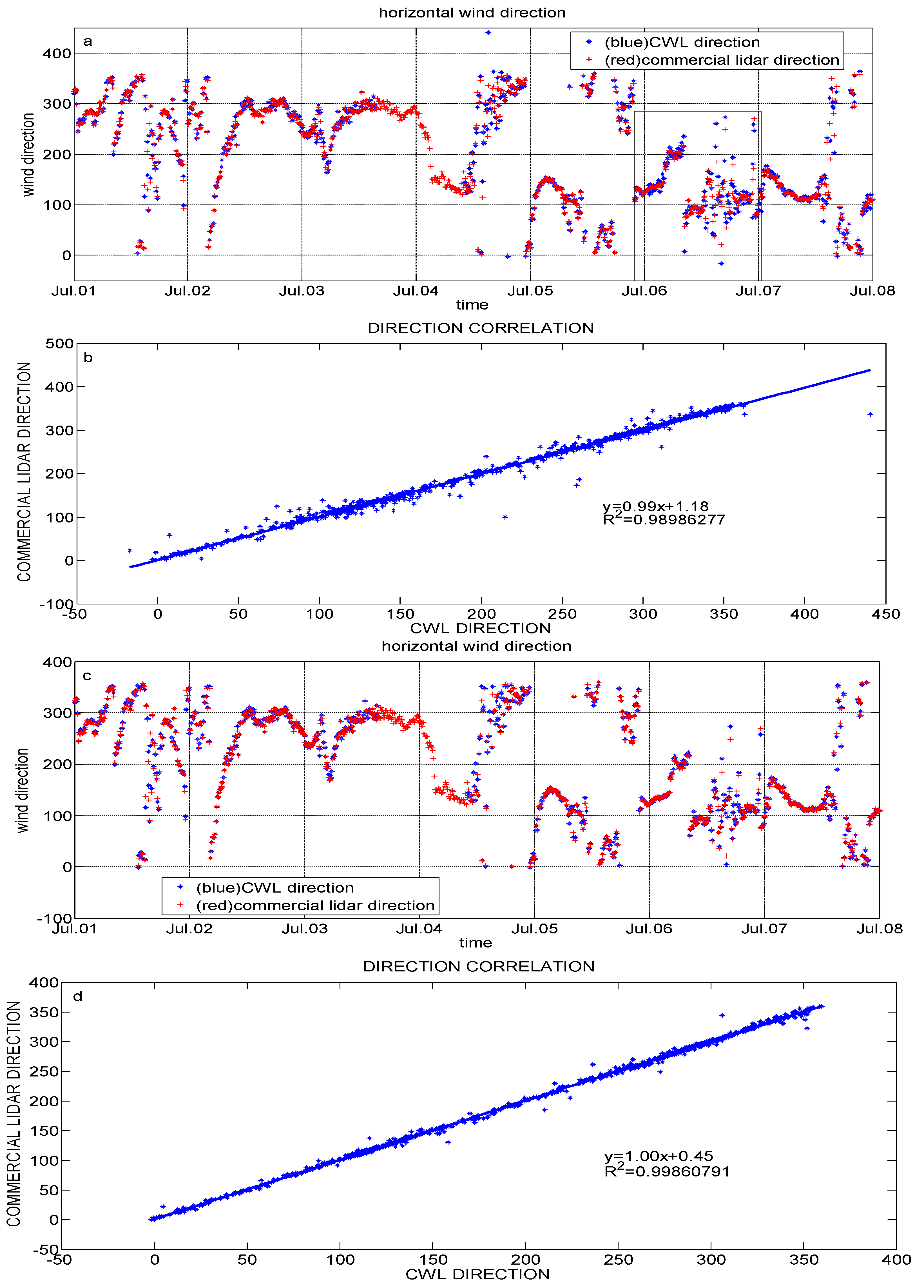
4.2.2. Horizontal Wind Direction

Figure 11 shows a comparison of the horizontal wind direction at 120 m during the test period. Figure 11a,b is associated with COG. The horizontal wind direction moves clockwise from east to west and then vacillates in the near-east direction on 6 June. The absolute deviation of the horizontal wind direction is 4.3585° and the correlation coefficient is 0.9899. Particularly, the absolute deviation of the horizontal wind direction is approximately 10.6362 on 6 June.

Figure 11c,d is related to the CR-CFAR method and evidently indicate that the extent of agreement of the horizontal wind direction on 6 June is higher than that of the commercial lidar. The absolute deviation of the horizontal wind direction is reduced to 2.7235°, which is much smaller than that after COG. Moreover, the absolute deviation of the horizontal wind direction during the campaign observation is 1.9382°, and the correlation coefficient is 0.9986.

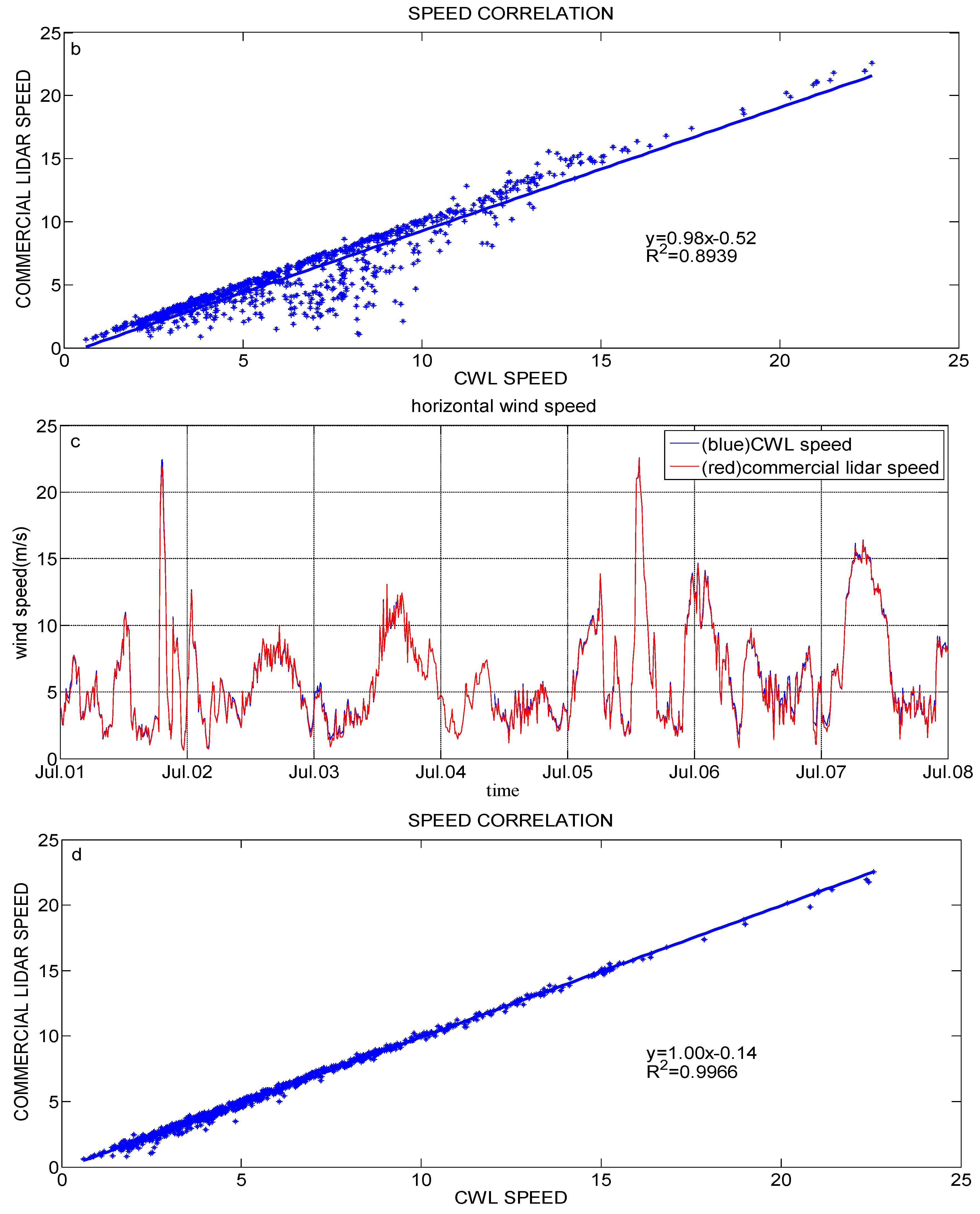
4.2.3. Correlations between the CWL and Commercial Lidar

Table 3. Correlations of horizontal wind speed and direction with the commercial lidar at different heights.

Height (m)	Horizontal Wind Velocity Correlation Based on COG	Horizontal Wind Velocity Correlation Based on CR-CFAR	Horizontal Wind Direction Correlation Based on COG	Horizontal Wind Direction Correlation Based on CR-CFAR
50	0.9969	0.9970	0.9994	0.9994
70	0.9989	0.9990	0.9988	0.9989
85	0.9959	0.9983	0.9989	0.9992
100	0.9787	0.9979	0.9967	0.9988
120	0.8938	0.9966	0.9899	0.9986
150	0.6335	0.9924	0.9563	0.9972
180	0.4065	0.9817	0.9156	0.9953
210	0.3448	0.9592	0.9027	0.9775
240	0.3663	0.9518	0.9313	0.9888
270	0.4657	0.9443	0.9046	0.9798
290	0.5007	0.9541	0.9032	0.9577

shows the correlations of the horizontal wind speed and horizontal wind direction at different heights using COG and CR-CFAR. By using COG, the wind speed correlations are more than 0.99 below the height of 85 m. However, this correlation gradually decreases to approximately 0.5 from the height of 100 m. At the same time, the correlation of the horizontal wind direction between 50 m and 100 m is more than 0.99; however, it rapidly decreases to approximately 0.9 as the height increases. This result shows that the wind field estimation after 100 m is not very accurate. The reason for the short detecting distance using COG is that the echo signal is relatively small on account of the dry climate and lower concentration of aerosol particles in the air.

The correlation of the horizontal wind speed can be increased to 0.99 from 50 m to 150 m using CR-CFAR. The maximum height at which the horizontal wind direction correlations are more than 0.99 can reach 180 m, which means the effective detection range increases by 65 m. It is worth mentioning that the detection ability of the commercial lidar at a low SNR is somewhat limited in this study. Therefore, the correlations at the height from 210 m to 290 m are relatively low (0.94 to 0.98).

4.3. Characteristics of Continuous Wind Field during Observation

Figure 12 presents the sequence diagrams of the horizontal wind speed during the experimental period. Figure 12a,b shows the variations of horizontal wind velocity with time using COG and CR-CFAR, respectively. From this figure, it is evident that the horizontal wind speeds after COG or CR-CFAR for a height less than 85 m are consistent. However, the wind field information above 85 m is not precisely detected using the COG method.

For example, the period between 05:00 and 10:00 on 7 June is marked as “C” in Figure 12a. In this period, there are very few aerosol particles in the atmosphere and the visibility is high. The CWL collected relatively smaller echo signals of the atmosphere. Although the meteorological records show that the wind speed is predominantly greater than 14 m/s in the mentioned period, the COG inversion result is slightly different. The period with a high wind speed is shorter than it should be. Therefore, the horizontal wind speed is more reliable by using the CR-CFAR method.

In addition, two sandstorms were observed and are shown as time segments, sandstorm A and sandstorm B, in Figure 12. In this paper, A is used as an example. Figure 12c,d shows COG and CR-CFAR, respectively. A sand dust storm began at 18:50 and ended at 19:50 on 1 June. The wind speed rapidly increased at the beginning of the storm; however, the wind speed decreased more slowly in the end when the air contained a large amount of sand and dust aerosol [34].

The brief start time and the yellow portion in Figure 12c,d show the consistency during this time. The end of the sandstorm using the CR-CFAR method is more uniform, which can be proven by the contrast between the red area of the upper-right corner of the dust storm center in Figure 12d and the corresponding yellow portion in Figure 12c. The center of the sand dust storm shown as a black part in Figure 12d was approximately 30 min using CR-CFAR, whereas in Figure 12c, it was approximately 10 min using COG. All of these observations show that more wind characteristics can be obtained from the inversion results using CR-CFAR than from COG.

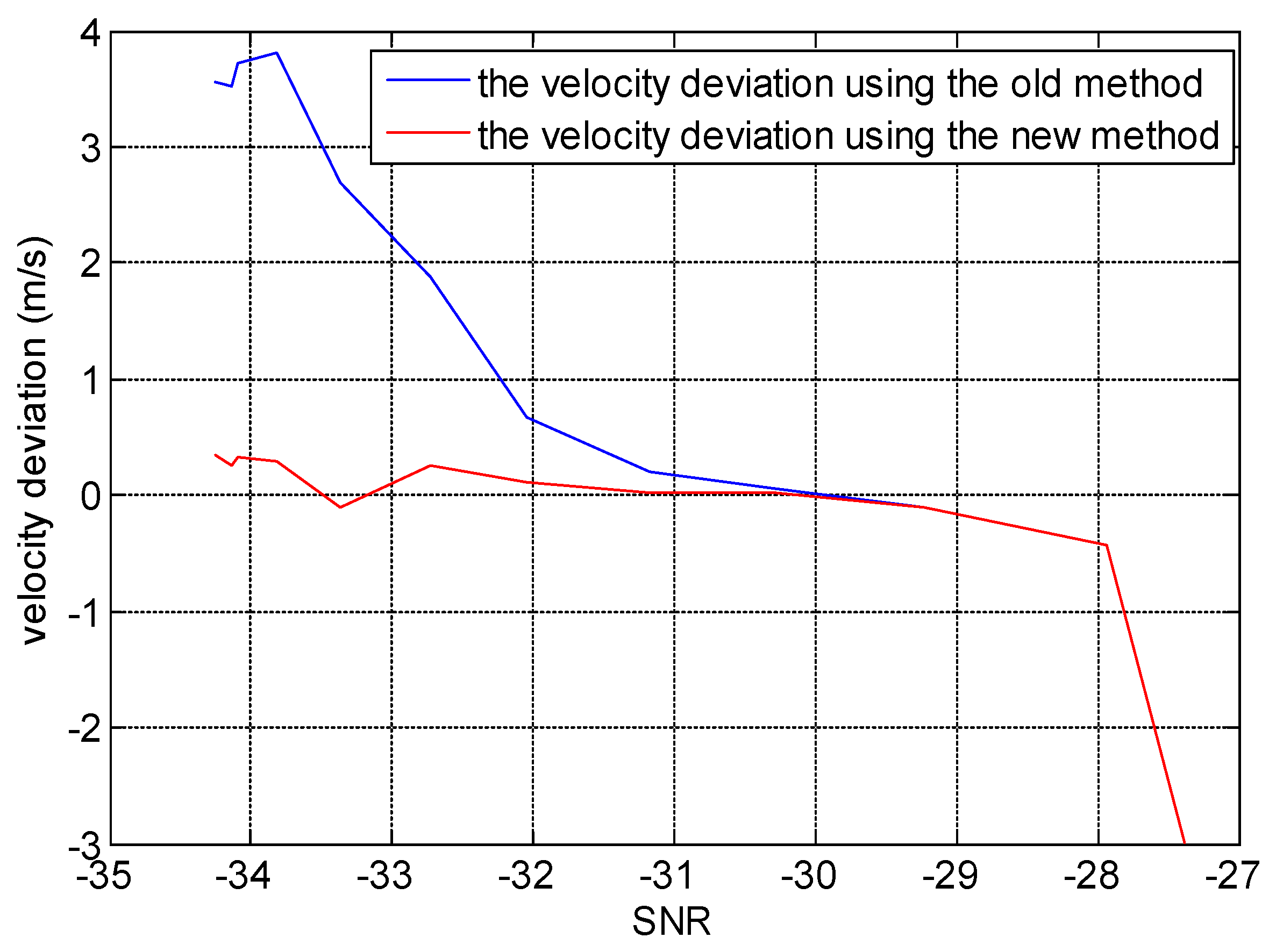
4.4. Error of CR-CFAR during Observation

The velocity deviation against the SNR during the whole experiment is displayed in Figure 13. The blue curve indicates the horizontal wind speed deviation obtained using COG, and the red curve is that obtained using CR-CFAR. For an SNR of −30 dB and lower, the horizontal wind velocity deviation obtained by using CR-CFAR is significantly smaller than that of the horizontal wind speed represented by the blue curve. For the case of an SNR of −28 dB and higher, the wind speed deviation is larger.

Table 4. Error of CWL using CR-CFAR at different heights.

Height (m)	Velocity Deviation (m/s)	Direction of Deviation (°)	Difference of Standard Deviation
70	−0.1102	−0.0179	−0.0140
85	0.0268	0.2295	0.0408
100	0.0194	0.3820	0.0147
120	0.1088	0.5382	0.2296

shows the CWL error at different heights compared with that of the commercial lidar. The horizontal wind speed deviation is less than 0.11 m/s, the deviation direction is less than 0.53°, and the standard deviation difference is less than 0.23. Especially for 85 m and 100 m, the velocity deviation values (0.0268 and 0.0194) are so small that the CWL and commercial lidar have similar detection ability.

5. Conclusions

In summary, the conventional COG method cannot produce unbiased estimates at a low SNR when analyzing CWL spectra. In this paper, a CR-CFAR is proposed as a spectral analysis method for unbiased estimation. Based on CFAR, the method is used to analyze the spectrum to solve the issue of weak signal discrimination in the widely used wind speed inversion method. We applied the new method to inversions of the wind field for one week. Comparisons between winds from CR-CFAR and COG were made using campaign observation data, which are indicated for practical CR-CFAR spectrum analyses, especially at a low SNR.

The results showed that the wind speed correlations using CR-CFAR at different altitudes were significantly improved compared to those for COG. The height at which the horizontal wind speed correlation was more than 0.99 changed from the original value of 85 m to 150 m. The relative deviation of the horizontal wind speed at 120 m decreased from the original 40.37% to 11.04%. The height at which the horizontal wind direction correlation was more than 0.99 changed from the original 100 m to 180 m. Through analysis of the continuous wind field, the derivation of the wind field in the sandstorm center was more accurate—and more wind characteristics were obtained—by using CR-CFAR. It can thus be concluded that CR-CFAR can be applied to CWL to improve the wind field inversion accuracy, which is expected to benefit future CWL applications.

References

1. Hangzhi, Y. Control Technology of Wind Turbine, China; Mechanics Industry Press: Beijing, China, 2002; p. 23. [Google Scholar]
2. Bao, D.; Chang, Z.; Dai, W.; Liu, Z.; Zhang, X.; Yao, M. Research on data processing method for power performance measurements of small wind turbine based on IEC standard. Renew. Energy Resour. 2014, 32, 649–654. [Google Scholar]
3. Lin, C. Theoretical analysis and experiment on power performance of doubly-fed wind power generator. Acta Energiae Sol. Sin. 2008, 3, 328–331. [Google Scholar]
4. Flesia, C.; Korb, C.L. Theory of the double-edge molecular technique for doppler lidar wind measurement. Appl. Opt. 2010, 38, 432–440. [Google Scholar] [CrossRef]
5. Xia, H.; Shangguan, M.; Wang, C.; Shentu, G.; Qiu, J.; Zhang, Q.; Dou, X.; Pan, J. Micro-pulse upconversion doppler lidar for wind and visibility detection in the atmospheric boundary layer. Opt. Lett. 2016, 41, 5218. [Google Scholar] [CrossRef] [PubMed]
6. Shangguan, M.; Xia, H.; Wang, C.; Qiu, J.; Shentu, G.; Zhang, Q.; Dou, X.; Pan, J.W. All-fiber upconversion high spectral resolution wind lidar using a fabry-perot interferometer. Opt. Lett. 2016, 24, 19322–19336. [Google Scholar] [CrossRef] [PubMed]
7. Akbulut, M.; Kimpel, F.; Gupta, S. Pulsed coherent fiber lidar transceiver for aircraft in-flight turbulence and wake-vortex hazard detection. Proc. SPIE Int. Soc. Opt. Eng. 2011. [Google Scholar] [CrossRef]
8. Kameyama, S.; Ando, T.; Asaka, K.; Hirano, Y.; Wadaka, S. Compact all-fiber pulsed coherent doppler lidar system for wind sensing. Appl. Opt. 2007, 46, 1953–1962. [Google Scholar] [CrossRef] [PubMed]
9. Cariou, J.P.; Augere, B.; Valla, M. Laser source requirements for coherent lidars based on fiber technology. C. R. Phys. 2006, 7, 213–223. [Google Scholar] [CrossRef]
10. Cariou, J.P.; Lolli, S.; Parmentier, R.; Sauvage, L. Validation of the new long range 1.5 μm wind lidar wls70 for atmospheric dynamics studies. Proc. SPIE Int. Soc. Opt. Eng. 2009. [Google Scholar] [CrossRef]
11. Diao, W.; Zhang, X.; Liu, J.; Zhu, X.; Liu, Y.; Bi, D. All fiber pulsed coherent lidar development for wind profiles measurements in boundary layers. Chin. Opt. Lett. 2014, 12, 71–74. [Google Scholar]
12. Bu, L.; Zhu, X.; Liu, J. All-fiber pulse coherent doppler lidar and its validations. Opt. Eng. 2015, 54. [Google Scholar] [CrossRef]
13. Bai, R.X.; Wang, B.Y.; Tong, P. Research status of laser doppler velocity radar technology. Laser Infrared 2016, 46, 249–253. [Google Scholar]
14. Hou, P.W.; Yang, L. Frequency estimation algorithm of sinusoid signal based on autocorrelation detection and energy centrobaric correction method. Sci. Technol. Eng. 2014, 14, 97–102. [Google Scholar]
15. Bao, B.; Yigang, H.E.; Tan, Y. Implementation of a complete synchronization digital frequency meter based on FPGA. J. Test Meas. Technol. 2008, 22, 99–102. [Google Scholar]
16. Roth, K.; Kauppinen, I.; Esquef, P.A.; Valimaki, V. Frequency warped Burg’s method for AR-modeling. In Proceedings of the 2003 IEEE Workshop on Applications of Signal Processing to Audio and Acoustics, New Paltz, NY, USA, 19–22 October 2003; pp. 5–8.
17. Berberidis, K.; Theodoridis, S. Efficient symmetric algorithms for the modified covariance method for autoregressive spectral analysis. IEEE Trans. Signal Process. 1993, 41, 43. [Google Scholar] [CrossRef]
18. Ma, K.; Zhang, Y.; Zhang, K. Performance analysis for CZT and ZFFT spectrum zoom and its FPGA realization. Comput. Meas. Control 2016, 24, 288–289. [Google Scholar]
19. Schwiesow, R.L.; Köpp, P.; Werner, C. Comparison of CW-lidar-measured wind values obtained by full conical scan, conical sector scan and two-point techniques. J. Atmos. Ocean. Technol. 1985, 2, 3–14. [Google Scholar] [CrossRef]
20. Fujii, T.D.; Fukuchi, T. Laser Remote Sensing; CRC Press of Taylor & Francis Group: Abingdon, UK, 2005. [Google Scholar]
21. Poor, H.V. An Introduction to Signal Detection and Estimation; Springer: Berlin, Germany, 2009. [Google Scholar]
22. Zhou, X.L.; Sun, D.S.; Zhong, Z.Q.; Wang, B.X.; Xia, H.Y.; Dong, J.J.; Shen, F.H.; Liu, D. Application of levenberg-marquardt algorithm in the wind lidar. Infrared Laser Eng. 2007, 36, 500–504. [Google Scholar]
23. Diao, W.F.; Liu, J.Q.; Zhu, X.P.; Liu, Y.; Zhang, X.; Chen, W.B. Study of All-Fiber Coherent Doppler Lidar Wind Profile Nonlinear Least Square Retrieval Method and Validation Experiment. Chin. J. Lasers 2015, 42, 330–335. [Google Scholar]
24. Beyon, J.Y.; Koch, G.J.; Singh, U.N.; Kavaya, M.J.; Serror, J.A. Development of the one-sided nonlinear adaptive Doppler shift estimation techniques. SPIE 2009, 7479. [Google Scholar] [CrossRef]
25. Koch, G.J.; Beyon, J.Y.; Barnes, B.W.; Petros, M.; Yu, J.; Amzajerdian, F.; Kavaya, M.J.; Singh, U.N. High-energy 2 μm Doppler Lidar for wind measurements. Opt. Eng. 2007, 46, 116201. [Google Scholar]
26. Zhu, X.P.; Liu, J.Q.; Diao, W.F.; Bl, D.C.; Zhou, J.; Chen, W.B. Study of coherent Doppler Lidar system. Infrared 2012, 33, 8–12. [Google Scholar]
27. Lank, G.W.; Chung, N.M. CFAR for homogeneous part of high-resolution imagery. IEEE Trans. Aerosp. Electron. Syst. 1992, 28, 370–381. [Google Scholar] [CrossRef]
28. Yan, Q.; Blum, R.S. Distributed signal detection under the Neyman-Pearson criterion. IEEE Trans. Inf. Theory 2001, 47, 1368–1377. [Google Scholar] [CrossRef]
29. Finn, H.M.; Johnson, R.S. Adaptive Detection Mode with Threshold Control as a Function of Spatially Sampled Clutter-Level Estimates. RCA Rev. 1968, 29, 414–464. [Google Scholar]
30. Tian, T. Sonar Technology; Harbin Engineering University Press: Harbin, China, 2010. [Google Scholar]
31. He, Y. Radar Target Detection and CFAR Processing; Beijing Tsinghua University Press: Beijing, China, 2011. [Google Scholar]
32. Wu, S.; Mei, X. Radar Signal Processing and Data Processing Technology; Electronic Industry Press: Beijing, China, 2008. [Google Scholar]
33. Lundquist, J.K.; Churchfield, M.J.; Lee, S.; Clifton, A. Quantifying error of lidar and sodar Doppler beam swinging measurements of wind turbine wakes using computational fluid dynamics. Atmos. Meas. Tech. 2015, 8, 907–920. [Google Scholar] [CrossRef]
34. Shen, J.; Li, Y.; Hu, T.; Yin, H. Causes and surface elements characteristics of a heavy sand-storm in 2010 in Minqin of Gansu, China. J. Desert Res. 2014, 34, 507–517. [Google Scholar]
Figure 1. Schematic of the CWL.
Atmosphere 07 00165 g001
Figure 2. Power spectrum at 85 m using the center of gravity method based on the maximum value method.
Atmosphere 07 00165 g002
Figure 3. Spectrum distribution at different heights: (a) SNR at different distances; (b) frequency spectrum at 85 m; (c) frequency spectrum at 150 m; and (d) frequency spectrum at 180 m.
Atmosphere 07 00165 g003
Figure 4. Model of the CR-CFAR method.
Atmosphere 07 00165 g004
Figure 5. Performance comparison of CA-CFAR and CR-CFAR.
Atmosphere 07 00165 g005
Figure 6. Line of sight wind speed at different directions. Line of sight wind speed in: (a) direction 2; (b) direction 4; (c) direction 6; and (d) direction 8.
Atmosphere 07 00165 g006
Figure 7. Geographical location and instrument layout.
Atmosphere 07 00165 g007
Figure 8. (a) Frequency spectrum at gate 12 with the background; and (b) frequency spectrum at gate 12 without the background.
Atmosphere 07 00165 g008
Figure 9. Signal point area at different gates after CR-CFAR.
Atmosphere 07 00165 g009
Figure 10. Horizontal wind speed at 120 m: (a) horizontal wind speed after COG; (b) correlation between the horizontal wind speed after COG and that of the commercial lidar; (c) horizontal wind speed after CR-CFAR; and (d) correlation between the horizontal wind speed after CR-CFAR and that of the commercial lidar.
Atmosphere 07 00165 g010aAtmosphere 07 00165 g010b
Figure 11. Horizontal wind direction at 120 m: (a) horizontal wind direction after COG; (b) correlation between the horizontal wind direction after COG and that of the commercial lidar; (c) horizontal wind direction after CR-CFAR; and (d) correlation between the horizontal wind direction after CR-CFAR and that of the commercial lidar.
Atmosphere 07 00165 g011
Figure 12. Horizontal wind speed of CWL. Horizontal wind velocity: (a) inverted from COG; (b) inverted from CR-CFAR; (c) during sandstorm A inverted from COG; and (d) during sandstorm A inverted from CR-CFAR.
Atmosphere 07 00165 g012
Figure 13. Horizontal wind speed deviation against SNR.
Atmosphere 07 00165 g013