Dynamics of Dew in a Cold Desert-Shrub Ecosystem and Its Abiotic Controls

Abstract

The temporal dynamics of dew formation in cold desert-shrub ecosystems are still poorly understood. We examined dew and its abiotic controls in a shrubland in northwestern China with continuous eddy-covariance measurements of latent heat fluxes gathered over the growing-season of 2012. The dew amount was larger in mid-summer than in spring and autumn, but the dew duration was shorter in summer (from ~10:00 p.m. to ~6:30 a.m.) than in spring and autumn (from ~8:30 p.m. to ~7:30 a.m.). Dew occurred on 85% (166 days) of growing-season days, with monthly means ranging from 0.09 to 0.16 mm day⁻¹. Dew was dominantly and positively controlled by Relative Humidity (RH), which explained 89% of its variation. Soil heat flux (G), air temperature (T_a), wind speed (W_s), Soil Water Content (SWC) and Vapor Pressure Deficit (VPD) also influenced dew formation. The most favorable conditions for dew formation were at T_a < 17 °C and RH > 75%. The Penman–Monteith equation predicted actual dew reasonably well. The predicted growing-season dew amount (21.3 mm) was equivalent to 7.2% and 8.9% of corresponding rainfall and evapotranspiration, respectively. It is suggested that dew could be a stable and continuous source of water that helps desert plants survive during warm summers.

1. Introduction

Dew occurs when moist air condenses on a substrate [1,2], as its surface temperature falls below the dew point temperature. Dew can originate from three separate sources: air (dewfall), plant (guttation), and soil (dewrise) [3]. Sufficient moisture in the air and intensive radiative cooling of the surface are two basic requirements for the formation of dew [4]. Relative humidity directly affects atmospheric visibility and the formation of clouds, fog, and dew [3,5,6]. In addition, the formation of dew is also indirectly affected by cloudiness [7], wind speeds, which may dampen the effect of radiative cooling by mechanically mixing the lower nocturnal boundary layer [1,8], soil water content [9], and the soil heat flux [6]. Likewise, soil texture [10], soil crusts [9], plant characteristics such as leaf area index [11], soil salinity [12], and elevation [13] all play a role in influencing the production of dew. However, there have been relatively few studies on the abiotic controls of dew in cold desert-shrub ecosystems.

Dew can be a stable and continuous source of water to plants through foliar uptake of moisture, as well as conserving soil water by reducing transpiration rates in early morning hours [14,15]. Dew is crucial to maintaining the water balance in some ecosystems and can efficiently reduce water loss caused by soil evaporation [3,6,16]. This is particularly the case for desert ecosystems [17,18], where rainfall is limited and soil moisture is often low.

Despite its ecological importance, the dynamics of dew in cold desert ecosystems are still poorly understood, mainly due to the lack of long-term measurements. Dryland (arid and semi-arid) accounts for 53% of China’s territory. Shrubland dominates this area by large and is an important ecosystem [19]. Understanding the dynamics of dew of desert ecosystem and its environmental control is, therefore, crucial to sustainably managing desert ecosystems.

Many attempts have been made to quantify dew in desert environments, using field measurements and models. Both have drawbacks. Field methods based on condensing surfaces [1], absorbent material or cloth plates [20], Duvdevani gauges [21] or dew harvesting [22] are used to quantify dew amount. Other field methods based on soil or air moisture sensors [23,24,25], leaf Wetness Sensors (WS) [17,26] or electrical impedance grids [27,28,29] are used to quantify the dew duration. Microlysimeters and Hiltner balances or electronic balances can be used for estimating both the duration and amount of dew [30,31]. Most of these field-based methods are labor intensive and thus limited in their use to acquire long-term continuous data. Furthermore, many devices either under- or over-estimate dew amount, because their reactive surfaces are composed of materials which respond differently than plant canopies. Theoretical methods to estimate dew can be broadly classified as empirical or analytical [22]. Empirical models are based on simple relationships with meteorological variables and are easy to use but can be highly site specific [32]. Conversely, analytical models based upon physical principles, such as the process-based Penman–Monteith equation [26,30], the cloud-based energy model [33], and a simple analytical formula based on a few meteorological data [34], can be applied in different environments but are more complex and often require data that are not readily available. The Penman–Monteith equation has the advantage of considering both the physiological and physical regulators of dew.

The Eddy-Covariance method (EC) has been applied in the examination of dew dynamics in many different ecosystems [6,26,35]. The EC method measures the latent heat flux (LE) between the biosphere and the atmosphere at the field scale [36,37,38], allowing for continuous long-term measurements [6,26]. However, EC measurements underestimate the flux during nighttime periods with low turbulence [39], and may thus underestimate dew.

Using the EC technique, we measured LE and the corresponding atmospheric water vapor content in a cold desert-shrub ecosystem dominated by Artemisia ordosica during the growing-season of 2012 (6 April to 18 October). Our primary objectives were: (1) to understand the dynamics of dew (duration, and amount); (2) to explore its abiotic controlling mechanisms; and (3) to evaluate the Penman–Monteith (P–M) equation for predicting dew.

2. Experiments

2.1. Site Description

Measurements were made in a 10-year-old shrubland at the Yanchi Research Station (37°42′31″N, 107°13′45″E, 1530 m above sea level (a.s.l.)), Ningxia, Northwest China. The research site is located at the southern edge of the Mu Us desert and is characterized by a mid-temperate semiarid continental monsoon climate. The site is dominated by a mixture of deciduous shrub species including Artemisia ordosica, Hedysarum mongolicum, Hedysarum scoparium and sparsely distributed Agropyron cristatum. The canopy height was about 1.4 m and the maximum Leaf Area Index (LAI) was 1.20 m²·m⁻² during the study period.

Mean annual temperature (1954–2004) is 8.1 °C in the research area and the frost-free season period is 165 days. Mean annual precipitation is 292 mm, 62% of which falls from July to September [40]. Mean annual pan evaporation is 2024 mm. The soil is sandy and the bulk density in the upper 10 cm is 1.54 ± 0.08 g·cm⁻³ (mean ± Standard Deviation (SD), n = 16, where n is the number of soil samples collected using a soil corer).

2.2. Measurements

The sensible heat flux H (W·m⁻²) and latent heat flux LE (W·m⁻²) were measured using the Eddy-Covariance method (EC). The measurement system consisted of a 3-D ultrasonic anemometer (CSAT3, Campbell Scientific Inc., Logan, UT, USA) and a fast response infrared gas analyzer (LI-7200, LI-COR Inc., Lincoln, NE, USA). The EC instruments were mounted at a height of 6.2 m on a scaffold tower and oriented in the prevailing wind direction (northwest). A data logger (LI-7550, LI-COR Inc., USA) was used to store 10 Hz data. The field site was flat and uniform for over 250 m in all directions from the flux tower. Footprint analysis using the Flux Source Area Model (FASM) showed that > 90% of the fluxes originated from within 200 m of the tower [41].

Daytime and nighttime was distinguished by PAR at the threshold of 5 µmol·m⁻² W·s⁻¹ [42,43,44]. The rate of nighttime dew was obtained directly from the EC measurements of negative LE at night (PAR < 5 µmol·m⁻²·s⁻¹). Daytime dew was derived from the negative LE starting from dawn or sunrise (i.e., PAR ≥ 5 µmol·m⁻²·s⁻¹). The dew rate E (mm·period⁻¹) was then estimated as:

$$E=LE/L$$

(1)

where L is the latent heat of vaporization (2450 J·kg⁻¹). Positive LE during nighttime and daytime (PAR ≥ 5 µmol·m⁻²·s⁻¹) was considered as evapotranspiration (ET).

Incident photosynthetically active radiation PAR (µmol·m⁻²·s⁻¹) was measured using a quantum sensor (PAR-LITE, Kipp and Zonen, Delft, the Netherlands). Net radiation R_n (W·m⁻²) was measured using a four-component radiometer (CNR-4, Kipp and Zonen, the Netherlands). Air temperature T_a (°C) and relative humidity RH (%) were measured with a thermohydrometer (HMP155A, Vaisala, Finland). Surface temperature T_s (°C) was measured with an infrared radiometer (SI-111, Campbell Scientific, Inc. Logan, UT, USA). Wind speed W_s (m·s⁻¹) was measured using a wind speed and direction sensor (034B, Met One Instruments Inc., Grants Pass, OR, USA). All these meteorological sensors were mounted on the tower at 6 m aboveground. Soil temperature T_10cm (°C) and soil water content SWC (m³·m⁻³) at 10 cm depth were monitored adjacent to the tower using ECH2O-5TE sensors (Decagon Devices, USA). Soil heat flux G (W·m⁻²) was computed as the sum of the fluxes measured at 10 cm depth by five soil heat plates (HFP01, Hukseflux Thermal Sensors, the Netherlands) and the rate of change in heat storage above the heat flux plates. The heat flux plates were installed at a distance of 5 m from the flux tower.

Rainfall measurements started from 15 May 2012. The measurements were done with a manual rain bucket before 22 July, and thereafter with a tipping bucket rain gauges (TE525WS, Campbell Scientific Inc., Logan, UT, USA) at distances of about 50 m around the tower. All micrometeorological variables were recorded every 30-min by data loggers (CR200X for PPT, CR3000 for all others, Campbell Scientific Inc., USA) from 6 April to 18 October, 2012. LAI was measured by destructive sampling at roughly weekly intervals within a 100 m × 100 m plot centered on the flux tower [44].

2.3. Post-Processing of Data

Half-hourly fluxes that suffered from inaccuracies caused by bad weather or instrument failure were excluded. In evaluating the P–M equation, LE values were excluded during calm nights (friction velocity u^* < 0.30 m·s⁻¹, where the u^* threshold was estimated following the ChinaFLUX standard method [45]). Gaps of less than 2 h in all variables were filled by linear interpolation. Longer gaps in LE were filled using the P–M equation, adjusted to match the EC measurements. Longer gaps in meteorological variables were filled by the Mean Diurnal Variation method (MDV) [36]. To assess the accuracy of LE, the Energy Balance Ratio (EBR) method was used. Nighttime energy balance closure was analyzed for the study period based on the regression between the measured available energy (R_n − G) and the sum of the EC turbulent heat fluxes (LE + H), where nighttime was delineated using PAR (i.e., as period with PAR < 5 µmol·m⁻²·s⁻¹). The nighttime EC measurements showed an acceptable energy-closure fraction of about 67% (slope = 0.67, R² = 0.91), which falls in the range of the values of 0.55 to 0.99 reported for FLUXNET [46], Our closure fraction of 0.67 indicates reasonable data quality but suggests our estimates of dew amount may be underestimated by as much as 33%. However, because the actual value of the closure fraction is uncertain, we did not apply an energy-closure adjustment to the measurements of dew amount, except in the evaluation of the dew estimates from the P–M equation. All data processing procedures were performed within Matlab (Version 7.5.0, The MathWorks, Natick, MA, USA).

2.4. Calculation of Bulk Parameters

The dew point temperature was calculated using the Magnus–Tetens approximation method [47] as:

$$\begin{array}{c}{T}_d=b\cdot \gamma (T_a,RH)/\left[a-\gamma \left(T_a,RH\right)\right]\\ \gamma (T_a,RH)=a\cdot T_a/(b+T_a)+\ln (RH/100)\end{array}$$

(2)

where T_d is dew point temperature (°C) and parameters a (17.27) and b (237.7) are constants. Daily minimum T_d was obtained from the 30-min T_d series. Dew days were defined in this work as days when daily minimum T_s was less than daily minimum T_d.

The P–M estimate of LE was computed as:

$$\lambda E=\frac{0.408\cdot \Delta (R_n-G)+\gamma \cdot \frac{C_n}{T_{\mathrm{s}}+273}\cdot W_s(e_s^0-e_a)}{\Delta +\gamma \cdot (1+C_d{W}_s)}$$

(3)

where Δ (kPa·K⁻¹) is the slope of the saturation vapor pressure versus air temperature curve (Equation (6)), γ is the psychrometric constant (0.055 kPa·°C⁻¹), C_n and C_d are reference parameters which vary by plant type, e_s° (kPa) is the saturated vapor pressure at surface temperature and e_a (kPa) is the ambient vapor pressure at the reference height of 6 m above the ground. In our study, C_n was set to 66 for both daytime and nighttime period [48], and C_d was set to 0.25 during the day and 1.7 at night.

The saturation and ambient vapor pressures were calculated with the Tetens formula [49]:

$$e_s^0=a\cdot \exp \left(\frac{b\cdot T_s}{T_s+c}\right)$$

(4)

$$e_a=RH\cdot a\cdot \exp \left(\frac{b\cdot T_a}{T_a+c}\right)$$

(5)

where a = 0.611 kPa, b = 17.502 (dimensionless), and c = 240.97 K. The value of Δ may be calculated as:

$$\Delta =\frac{b\cdot c\cdot e_s^0}{{(c+T_s)}^2}$$

(6)

2.5. Data Analyses

Days with rain were screened from the analysis. One-way analysis of variance (ANOVA) was used to test for differences among months in the time of dew commencement and cessation. Daily values were considered as replicates within each month (test groups). Path analysis was used to analyze the comprehensive effects of abiotic factors on dew formation. Nonlinear regression was conducted based on daily non-gapfilled data to analyze the relationship between dew and different environmental factors. The regression analyses were limited to the mid-growing season (June–August) to exclude the confounding effects of plant phenology. The dew values were bin-averaged for each abiotic factor, with a minimum of five data points required for a valid bin. Threshold values for some fits were identified when the fitted relationship was asymptotic. Regression analysis was also used to examine the relationship between EC measurements and P–M equation estimates of dew amount. Regression significance was evaluated using the F statistic at a significance level of 0.05. Root-Mean-Square Error (RMSE) and Bias Error (BE) (estimated minus measured values) were used to evaluate the goodness of fit of the P–M equation. All the statistical analyses were performed using the SPSS 20.0 program for windows (SPSS 20.0 Inc., Chicago, IL, USA).

3. Results

3.1. Seasonal Changes in Environmental Variables

Environmental variables observed from 6 June to 18 October (196 days) showed clear seasonal patterns both for day- and nighttime values (Figure 1). Diurnal values of air temperature (T_a), surface temperature (T_s), wind speed (W_s), soil heat flux (G) and vapor pressure deficit (VPD) were all higher than the values at night, but opposite to RH. The mean T_a at night ranged from 1.94 °C on 12 April to 21.35 °C on 29 July (Figure 1a). The mean T_s at night had a minimum of −2.36 °C on 12 April and a maximum of 20.7 °C on 29 July (Figure 1b). The mean RH at night was 64.3 ± 18.8%, with 117 days being greater than 60% and 90 days greater than 70% (Figure 1c). The mean W_s at night had a maximum of 5.17 m·s⁻¹ and a minimum of 0.59 m·s⁻¹, averaging 2.18 ± 0.93 m·s⁻¹ over the growing season (Figure 1d). Of all the nights with dew, the number of nights with W_s < 3.0 m·s⁻¹ were 150, accounting for 90% of the nights with dew. The number of nights with W_s < 1.0 m·s⁻¹ accounted for 6.6% of dew nights. Accumulated G at night reached a maximum of 84.0 W·m⁻² on 1 June and a minimum of −273.2 W·m⁻² on 1 September. Eighty-three percent of nights had G values ≤ 0 during the observation period (Figure 1e). Total rainfall was 296 mm over the growing season. There were three big rainfall events of ≥ 20 mm·day⁻¹ over the growing season, with the largest being 50 mm·day⁻¹ on 27 June (Figure 1f). Soil Water Content (SWC) at a 10 cm depth followed the pattern of rainfall and there was no significant difference between means during the day and at night during the measurement period (Figure 1f). The nightly mean VPD reached a maximum of 1.29 kPa on 13 June and the minimum of VPD is 0.06 kPa on 4 May, averaging 0.55 ± 0.29 kPa over the season (Figure 1g).

3.2. Seasonal Changes in Dew

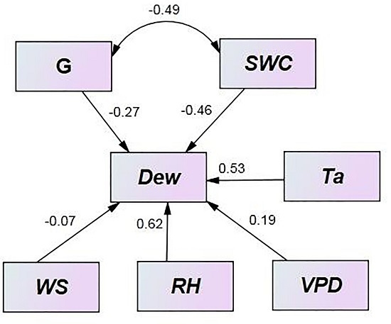
Dew amounts varied over the growing season (Figure 2), with higher values in mid-summer (June–August) and lower values in spring and autumn. The maximum daily dew amount was 0.16 mm on 21 September, and the minimum was 2.4 × 10⁻³ mm on 13 May, with a mean dew amount of 0.049 ± 0.04 mm over the observational period. The maximum monthly mean daily dew amount was 0.08 mm in July and the minimum was 0.03 mm in May. The maximum monthly mean daytime dew amount was 0.04 mm in July and the minimum was 0.004 mm in May.

The total number of dew days was 166, which accounted for 85% of the growing season. Mean daily dew duration varied by month (Figure 3). Daytime dew duration was longest in July, and shortest in April and May, most variable in July (from 0.5 to 7 h), and least variable in May (0.5 to 2 h) (Figure 3a). Nighttime duration was longest in October, most variable in April and August (from 1 to 9.5 h), and least variable in October (3.5 to 10 h) (Figure 3b). The average duration for daytime and nighttime were 1.3 h·day⁻¹ and 6.2 h·day⁻¹, respectively.

In autumn (September and October), dew commencement was earliest and cessation was latest (

Table 1. Monthly dew estimates, including: mean start and end times (rain-free days only), mean daily dew amount (after filling of gaps), monthly total (after filling of gaps), monthly evapotranspiration (ET), rainfall, ratio of dew to rainfall, and ratio of water input (dew + rainfall) to ET, for a desert-shrub ecosystem in Yanchi, Ningxia.

Month	Start Time (HH: MM p.m)	End Time (HH: MM a.m)	Daily Amount (mm·day−1)	Monthly Amount (mm)	ET (mm)	Rainfall (mm)	Dew: Rainfall (%)	Dew + Rainfall: ET (%)
April	8:40	7:10	0.16	3.9	80	--	--	5
May	9:20	6:30	0.11	3.1	75	22	14	33
June	10:40	6:30	0.09	2.1	67	83	2	127
July	9:50	6:40	0.12	2.7	42	63	4	156
August	9:30	6:55	0.16	4.3	63	42	10	74
September	8:40	7:25	0.11	2.8	55	72	4	136
October	8:20	7:30	0.14	3.0	32	15	15	54
Total	--	--	--	21.3	238	296	7	133

). In the summer, dew commenced later and ceased earlier. Significant inter-month variation in mean daily commencement times were observed (P = 0.000, ANOVA). However, there were no clear inter-month differences in dew cessation (P = 0.108, ANOVA).

3.3. Control of Dew

Path analysis of the effect of meteorological factors on dew amount (Figure 4) revealed the strong positive effect of RH, T_a, a moderate negative effect of SWC, a weak positive effect of VPD, and weak negative effects of G and W_s. Among these factors, the influence of RH was strongly dominant.

Nonlinear regressions of daily dew amount against environmental variables during the peak-growing season are shown in Figure 5. Dew increased with increasing T_a when T_a ≤ 17 °C, and then remained constant at T_a > 17 °C. Dew stayed constant and relatively low when RH ≤ 75%, and then increased sharply when RH > 75%. The independent variables T_a and RH individually explained 54% and 89%, respectively, of the variations in daily dew amount (Figure 5a,b). The independent variables W_s, G, SWC and VPD individually explained 36%, 68%, 56% and 77% of the variations in dew, respectively (Figure 5c–f). In general, dew decreased with increasing W_s, SWC, VPD and G (which is vector, so that negative values means upward soil heat flux and positive means downward).

There was a significant positive relationship between daily rainfall amount and dew amount on the first day after rainfall (R² = 0.81, p < 0.05, Figure 6). To further examine the effects of rainfall events on dew, we examined dew during six consecutive days (day of year (DOY) 178–183), including two rainfall days (DOY 179–180), the day prior (178) and the three days after (181–183) (Figure 7). On the two days with rain, all rain (61 mm) fell during daytime hours. The SWC increased sharply during the rainy day DOY 179, and then decreased slowly afterwards. The RH increased sharply on DOY 179, and then remained almost saturated during the day DOY 180 and 181. T_a remained relatively low during the two rainy days and increased, showing a clear day-night difference on the day DOY 181–183. Dew was markedly increased on the first day (DOY 181) following rain compared to the day before rain.

3.4. Contribution of Dew to the Water Balance

Energy-closure-adjusted values of LE were used to evaluate the P–M equation (Figure 8). The closure adjustment was applied by dividing the LE values by the observed closure fraction of 0.67. The P–M equation estimates of dew amount were more closely correlated with the measured dew over daily than hourly time scales (Figure 8a,b; hourly R² = 0.37, P < 0.05 and daily R² = 0.73, P < 0.05). The fitted lines were reasonably close to 1:1 line both at the hourly and daily scale, with a slope of 1.11 at the hourly scale and 1.21 at the daily scale. The RMSE and BE were small, with values of 1.9 × 10⁻⁴ and 3.7 × 10⁻³ mm at hourly scale, and 5.4 × 10⁻³ and 1.80 × 10⁻³ mm at the daily scale, respectively. Residuals showed that the P–M equation was able to estimate dew reasonably well at both timescales (Figure 8c,d).

After applying the relationship between estimated and measured dew to fill gaps in daily dew, and conducting a similar daytime analysis to fill gaps in day- and nighttime ET (Figure 9a), the values were summed over the study period. The total dew was 21.3 mm, which accounts for 8.9% of seasonal ET (238 mm), and 7.2% of corresponding rainfall (296 mm) over the same period. At a monthly time scale, the ratio of dew to rainfall varied significantly from 2% in June to 15% in October (Table 1). The ratio of inputs to outputs (dew plus rainfall to ET) varied greatly from 5% in April to 156% in July demand (Table 1). The monthly contribution of dew to ET was greater during July–October than April–June (Figure 9b).

4. Discussion

4.1. Measurements Issues and Uncertainties

EC measurements of LE are subject to moderate uncertainty, and the measurement of nighttime flux is particularly challenging [26,50], The EC technique fails during periods of low wind speed at night and routinely under measures of LE at higher wind speeds, with energy-closure fractions of less than one [46]. To compensate for these problems, we have excluded calm nights from the analysis using a very conservative u^* threshold of 0.30 m·s⁻¹. We have also evaluated energy-balance closure at night and found a closure fraction (i.e., (H + LE)/(R_n − G)) of 0.67, which is comparable to other studies. However, this fraction was not used to adjust the dew amount because it is subject to high uncertainty. Although there is moderate uncertainty in the growing season total dew amount related to the uncertainty in LE, the process relationships from this study, such as shown in Figure 4 and Figure 5, are robust and are not affected by the uncertainties in the energy-closure adjustments.

The meteorological sensors in this study were mounted at 6 m height, which is higher than the standard height for meteorological measurements and higher than previous studies. The height difference between this study and previous studies may account for the lower RH threshold (75%) for dew in this study, because of the steep gradients in RH that exist near the surface at night. Fortunately, the higher sensor height in this study does not invalidate the functional relationships in, e.g., Figure 5, but it may alter the values of the fitted parameters. The dew estimates from eddy-covariance reflected the dynamics of dew well and can be used to understand its controlling mechanisms.

In addition, the P–M equation was shown to fit the EC dew measurements reasonably well when a u* threshold of 0.30 m·s⁻¹ and an energy closure adjustment of 1/0.67 were used. This suggests that the P-M equation is suitable to estimate dew in the study area.

4.2. The Formation Characteristics of Dew

Our study site is in the south edge of the Mu Us desert (also called the Mu Us sandland, 1200–1600 m a.s.l.), which lies in a critical geographic transition zone between arid and semiarid climates, and between agricultural and pastoral land uses. Compared to the deserts in its west (such as the Tengger desert, annual rainfall 116–148 mm), Mu Us desert has larger rainfall (annual 250–440 mm) and abundant ground and underground water. Haba Lake, which is 30 km from our study site, supplies moisture with southwest wind blowing in summer. We think that the vapor at our site might be from Haba Lake and soil water.

The measurements by EC technique in our study included dewfall from the atmosphere and dewrise from evaporated soil water (frequently termed distillation), as well as water vapor brought to the surface by turbulent diffusion [51]. Considering the dry soil moisture conditions (most of nightly SWC were below 0.09 m³·m⁻³) and the sparse plants (the cover of plants was 56%) at our site, dew amount from soil and plants were comparatively small. Therefore, dewfall predominated in dew formation [3].

Negative latent heat fluxes at night were considered as dew [6]. We found that dew occurred on 85% of the nights during our study period, which is higher than other estimates of 33% to 78% [5,17,26,32,52,53]. The monthly mean dew amount was higher in mid-summer than spring or autumn (Figure 2) probably because rainfall was concentrated in mid-summer, increasing RH and decreasing VPD and thus enhancing dew. Dew duration increased from May to October. Although average daytime dew duration was small compared with that at nighttime, it can help wet the plant canopy and reduce surface temperature in the morning. The earlier dew commencement and later dew cessation times in spring and autumn compared to summer (Figure 3, Table 1) was due in part to the shorter summer nights [5].

4.3. Control of Dew

Our present results for a desert-shrub ecosystem show that RH was the main environmental factor in controlling dew formation during the growing season. However, dew was also controlled by T_a, VPD, G, SWC and W_s. At night, higher temperature led to higher water vapor in the environment, and thus higher water condensation. Larger the VPD means lower the vapor pressure in the air, the lower vapor pressure may decrease the water vapor of air, and then decrease the dew amount. Larger G at night probably means higher surface and soil temperature, which can also positively influence vapor pressure and water vapor of air, thus increasing the dew amount [6] and decrease the SWC. Low soil SWC led to low thermal conductivity, thus leading to higher soil temperature difference between day and night and thus facilitating dew formation. High correlation of dew with RH (R² = 0.89) and path analysis result indicate that RH was an important factor in controlling dew. This result is similar to previous reports [5,32,34,54]. We found that dew was low and approximately constant at RH below 75%, and increased sharply when RH exceeded 75%. This threshold for dew formation was lower than that reported by Shaw [55] who found a good correlation between dew formation and RH above 85%, and Smith [56] who found an RH threshold of 90% for dew occurrence. The reason might be that our study area is a semi-arid desert area, where the water vapor content in the air is very low, making RH an important limited factor for the formation of dew. Alternatively, it might be related to difference in RH observation height and instruments; our observation of 6 m is much higher than most, and our instrument, unlike others, did not overestimate RH at high values. The results of different studies show that RH of 100% is not an essential condition for dew formation. Light wind favors dew formation [57] as it can bring moisture which facilitates dew formation and extend the dew duration. Previous studies have shown that most dew events occur at W_s below 2 m·s⁻¹ [54,58]. Other studies have also shown that a wind speed of 3–3.6 m·s⁻¹ is favorable for dew formation, while a wind speed greater than 4.7 m·s⁻¹ adversely affects dew formation [8]. In our study, the maximum daily W_s and the daily mean W_s during dew formation were 4.16 m·s⁻¹ and 2.18 ± 0.93 m·s⁻¹, respectively, similar to other studies.

Dew relies on moisture supplied from the atmosphere. Rainfall may increase RH and decrease VPD in the air, thus increasing the dew amount [7]. Our finding of a positive relationship between daily rainfall and dew on the following day, is in agreement with previous reports [59]. Dew was markedly increased after rainfall day supporting the hypothesis that dew in semi-arid environments is enhanced immediately after rainfall.

4.4. Contribution of Dew to the Water Balance

Dew is an important component of the water balance in arid and semi-arid ecosystems over large time scales of months to years [16]. The ratio of growing season dew to rainfall was 7%, which is much smaller than reported in desert environments: 35% for the Negev Desert, Israel [60,61], 37% for Rajasthan Desert, India [13], 67% in a desert riparian forest ecosystem on the eastern edge of the Taklimakan desert [6] and 40% in a coastal site in Mirleft, Morocco [32]. In addition, as distillation stemmed from rain may be considered as an additional source of moisture, which would be calculated as dewfall, thus leading to the overestimation of dew than actual. So the actual ratio of dew in the growing season to corresponding rainfall may be a little smaller than 7%. The three driest months in our study, with rainfall < 30 mm (April, May and October), had slightly higher rainfall to dew ratios of 15% (Table 1). Over the growing season (196 days), dew occurred on 166 days, whereas rainfall occurred on only 29 days. These findings suggest that although dew amounts are relatively small in our study site, they are a stable and continuous source of water for ET in desert area [26]. Dew combined with rainfall as water input met the ET demand at our study site, thus maintaining the growth of desert woody plants. In our study dew increased from July to October, whereas ET decreased during this period, indicating that transpiration was decreasing in contrast to the pattern observed with dew [62].

Dew as a part of water and heat exchange, plays an important role in eco-environment in arid and semi-arid area. Dew can wet the surface layer of plants, reduce the temperature of plant leaves, supplement the water transpired. Dew may take place either on the shrubs and annuals or on the bare soil or crust, Jacobs et al. (2002) indicated that moisture contributed by dew promotes crust development [30]. The research of Lange et al. (1992) found 0.1 mm of dew marks the threshold of dew availability for net photosynthesis necessities of biological soil crusts [63]. This is similar to the findings reported by Veste et al.(2008) [18]. Uclés et al. (2014) showed that bare soil and crusts contribute 36% of the dewfall in a coastal-steppe ecosystems along the Mediterranean coast [17]. However, other studies, which had measured dew above the ground, found almost little on the soil or crusts [2,61,64]. The reason may be that dew at the soil surface was further impeded due to the soil thermal properties [65]. The higher dew amount (0.13 mm·night⁻¹ gapfilled by Penman–Monteith equation) in our research area may help with the water need for photosynthesis of biological soil crusts. However, due to the uncertainties of dew amount estimated by EC technique, the overall contribution of dew amount to the crust photosynthesis needs further study.

5. Conclusions

Eddy-covariance measurements of dew in a cold desert-shrub ecosystem in Ningxia, China, showed dew amounts ranging from 0.09–0.16 mm·day⁻¹ over the growing season, with higher values in summer than spring or autumn. Dew was observed on 85% of growing season days. Seasonal changes in the dew amount were mainly driven by Relative Humidity (RH), which had a strong positive effect on dew. Soil heat flux (G), air temperature (T_a), wind speed (W_s), Soil Water Content (SWC) and Vapor Pressure Deficit (VPD) also influenced dew formation. Water provided by both dew and rainfall adequately met evapotranspiration needs at our site. Dew is an indispensable source of water for plant survival in semi-arid environments and would be even more important under current scenarios of climate warming and increasing drought in xeric habitats.

References

1. Beysens, D. The formation of dew. Atmos. Res. 1995, 39, 215–237. [Google Scholar] [CrossRef]
2. Agam, N.; Berliner, P. Dew formation and water vapor adsorption in semi-arid environments—A review. J. Arid Environ. 2006, 65, 572–590. [Google Scholar] [CrossRef]
3. Pan, Y.; Wang, X.; Zhang, Y. Dew formation characteristics in a revegetation-stabilized desert ecosystem in shapotou area, Northern China. J. Hydrol. 2010, 387, 265–272. [Google Scholar] [CrossRef]
4. Xiao, H.; Meissner, R.; Seeger, J.; Rupp, H.; Borg, H.; Zhang, Y. Analysis of the effect of meteorological factors on dewfall. Sci. Total Environ. 2013, 452, 384–393. [Google Scholar] [CrossRef] [PubMed]
5. Zangvil, A. Six years of dew observations in the Negev desert, Israel. J. Arid Environ. 1996, 32, 361–371. [Google Scholar] [CrossRef]
6. Hao, X.; Li, C.; Guo, B.; Ma, J.; Ayup, M.; Chen, Z. Dew formation and its long-term trend in a desert riparian forest ecosystem on the eastern edge of the Taklimakan Desert in China. J. Hydrol. 2012, 472, 90–98. [Google Scholar] [CrossRef]
7. Chen, L.; Meissner, R.; Zhang, Y.; Xiao, H. Studies on dew formation and its meteorological factors. J. Food. Agric. Environ. 2013, 11, 1063–1068. [Google Scholar]
8. Monteith, J. Dew. Quart. J. Roy. Meteorol. Soc. 1957, 83, 322–341. [Google Scholar] [CrossRef]
9. Liu, L.; Li, S.; Duan, Z.; Wang, T.; Zhang, Z.; Li, X. Effects of microbiotic crusts on dew deposition in the restored vegetation area at Shapotou, northwest China. J. Hydrol. 2006, 328, 331–337. [Google Scholar] [CrossRef]
10. Li, X.-Y. Effects of gravel and sand mulches on dew deposition in the semiarid region of China. J. Hydrol. 2002, 260, 151–160. [Google Scholar] [CrossRef]
11. Feng, Q.; Gao, Q. Preliminary study on condensation water in semi-humid sandyland. Arid Zone Res. 1995, 12, 72–77. (In Chinese) [Google Scholar]
12. Guo, Z.; Liu, J. An overview on soil condensate in arid and semiarid regions in China. Arid Zone Res. 2005, 4, 028. [Google Scholar]
13. Subramaniam, A.; Rao, A.K. Dew fall in sand dune areas of India. Int. J. Biometeorol. 1983, 27, 271–280. [Google Scholar] [CrossRef]
14. Goldsmith, G.R.; Matzke, N.J.; Dawson, T.E. The incidence and implications of clouds for cloud forest plant water relations. Ecol. lett. 2013, 16, 307–314. [Google Scholar] [CrossRef] [PubMed]
15. Munné-Bosch, S.; Nogués, S.; Alegre, L. Diurnal variations of photosynthesis and dew absorption by leaves in two evergreen shrubs growing in Mediterranean field conditions. New Phytol. 1999, 144, 109–119. [Google Scholar]
16. Lekouch, I.; Muselli, M.; Kabbachi, B.; Ouazzani, J.; Melnytchouk-Milimouk, I.; Beysens, D. Dew, fog, and rain as supplementary sources of water in south-western Morocco. Energy 2011, 36, 2257–2265. [Google Scholar] [CrossRef] [Green Version]
17. Uclés, O.; Villagarcía, L.; Moro, M.; Canton, Y.; Domingo, F. Role of dewfall in the water balance of a semiarid coastal steppe ecosystem. Hydrol. Process. 2014, 28, 2271–2280. [Google Scholar] [CrossRef]
18. Veste, M.; Heusinkveld, B.; Berkowicz, S.; Breckle, S.-W.; Littmann, T.; Jacobs, A. Dew formation and activity of biological soil crusts. In Arid dune ecosystems; Springer: Berlin, Germany, 2008; pp. 305–318. [Google Scholar]
19. Jia, X.; Zha, T.; Gong, J.; Wu, B.; Zhang, Y.; Qin, S.; Chen, G.; Feng, W.; Kellomäki, S.; Peltola, H. Energy partitioning over a semi-arid shrubland in northern China. Hydrol. Process. 2015. [Google Scholar] [CrossRef]
20. Kidron, G.J. Analysis of dew precipitation in three habitats within a small arid drainage basin, Negev highlands, Israel. Atmos. Res. 2000, 55, 257–270. [Google Scholar] [CrossRef]
21. Duvdevani, S. An optical method of dew estimation. Quart. J. Roy. Meteorol. Soc. 1947, 73, 282–296. [Google Scholar] [CrossRef]
22. Tomaszkiewicz, M.; Abou Najm, M.R.; Beysens, D.; Alameddine, I.; El-Fadel, M. Dew as a sustainable non-conventional water resource: A critical review. Environ. Rev. 2015, 23, 425–442. [Google Scholar] [CrossRef]
23. Bunnenberg, C.; Kühn, W. An electrical conductance method for determining condensation and evaporation processes in arid soils with high spatial resolution. Soil Sci. 1980, 129, 58–66. [Google Scholar] [CrossRef]
24. Schmitz, H.F.; Grant, R.H. Precipitation and dew in a soybean canopy: Spatial variations in leaf wetness and implications for Phakopsora pachyrhizi infection. Agric. Forest Meteorol. 2009, 149, 1621–1627. [Google Scholar] [CrossRef]
25. Cosh, M.H.; Kabela, E.D.; Hornbuckle, B.; Gleason, M.L.; Jackson, T.J.; Prueger, J.H. Observations of dew amount using in situ and satellite measurements in an agricultural landscape. Agric. Forest Meteorol. 2009, 149, 1082–1086. [Google Scholar] [CrossRef]
26. Moro, M.; Were, A.; Villagarcía, L.; Cantón, Y.; Domingo, F. Dew measurement by eddy covariance and wetness sensor in a semiarid ecosystem of SE Spain. J. Hydrol. 2007, 335, 295–302. [Google Scholar] [CrossRef]
27. Pedro, M.; Gillespie, T. Estimating dew duration. I. Utilizing micrometeorological data. Agric. For. Meteorol. 1981, 25, 283–296. [Google Scholar] [CrossRef]
28. Gleason, M.; Taylor, S.; Loughin, T.; Koehler, K. Development and validation of an empirical model to estimate the duration of dew periods. Plant Dis. 1994, 78, 1011–1016. [Google Scholar] [CrossRef]
29. Pedro, M.; Gillespie, T. Estimating dew duration. II. Utilizing standard weather station data. Agric. For. Meteorol. 1981, 25, 297–310. [Google Scholar] [CrossRef]
30. Jacobs, A.F.; Heusinkveld, B.G.; Berkowicz, S.M. A simple model for potential dewfall in an arid region. Atmos. Res. 2002, 64, 285–295. [Google Scholar] [CrossRef]
31. Muselli, M.; Beysens, D.; Marcillat, J.; Milimouk, I.; Nilsson, T.; Louche, A. Dew water collector for potable water in Ajaccio (Corsica Island, France). Atmos. Res. 2002, 64, 297–312. [Google Scholar] [CrossRef]
32. Lekouch, I.; Lekouch, K.; Muselli, M.; Mongruel, A.; Kabbachi, B.; Beysens, D. Rooftop dew, fog and rain collection in southwest Morocco and predictive dew modeling using neural networks. J. Hydrol. 2012, 448, 60–72. [Google Scholar] [CrossRef]
33. Madeira, A.; Kim, K.; Taylor, S.; Gleason, M. A simple cloud-based energy balance model to estimate dew. Agric. For. Meteorol. 2002, 111, 55–63. [Google Scholar] [CrossRef]
34. Beysens, D. Estimating dew yield worldwide from a few meteo data. Atmos. Res. 2016, 167, 146–155. [Google Scholar] [CrossRef]
35. Vermeulen, A.; Wyers, G.; Römer, F.; Van Leeuwen, N.; Draaijers, G.; Erisman, J. Fog deposition on a coniferous forest in the Netherlands. Atmos. Environ. 1997, 31, 375–386. [Google Scholar] [CrossRef]
36. Falge, E.; Baldocchi, D.; Olson, R.; Anthoni, P.; Aubinet, M.; Bernhofer, C.; Burba, G.; Ceulemans, R.; Clement, R.; Dolman, H. Gap filling strategies for long term energy flux data sets. Agric. For. Meteorol. 2001, 107, 71–77. [Google Scholar] [CrossRef]
37. Aubinet, M.; Grelle, A.; Ibrom, A.; Rannik, Ü.; Moncrieff, J.; Foken, T.; Kowalski, A.; Martin, P.; Berbigier, P.; Bernhofer, C. Estimates of the Annual Net Carbon and Water Exchange of Forests: The EUROFLUX Methodology. Adv. Ecol. Res. 1999, 30, 113–175. [Google Scholar]
38. Aubinet, M.; Clement, R.; Elbers, J.; Foken, T.; Grelle, A.; Ibrom, A.; Moncrieff, J.; Pilegaard, K.; Rannik, Ü.; Rebmann, C. Methodology for data acquisition, storage, and treatment. In Fluxes of Carbon, Water and Energy of European Forests; Springer: Berlin, Germany, 2003; pp. 9–35. [Google Scholar]
39. Papale, D.; Reichstein, M.; Aubinet, M.; Canfora, E.; Bernhofer, C.; Kutsch, W.; Longdoz, B.; Rambal, S.; Valentini, R.; Vesala, T. Towards a standardized processing of net ecosystem exchange measured with eddy covariance technique: Algorithms and uncertainty estimation. Biogeosciences 2006, 3, 571–583. [Google Scholar] [CrossRef]
40. Wang, B.; Zha, T.; Jia, X.; Wu, B.; Zhang, Y.; Qin, S. Soil moisture modifies the response of soil respiration to temperature in a desert shrub ecosystem. Biogeosciences 2014, 11, 259–268. [Google Scholar] [CrossRef]
41. Schmid, H. Experimental design for flux measurements: Matching scales of observations and fluxes. Agric. For. Meteorol. 1997, 87, 179–200. [Google Scholar] [CrossRef]
42. Zha, T.; Kellomäki, S.; Wang, K.Y.; Rouvinen, I. Carbon sequestration and ecosystem respiration for 4 years in a scots pine forest. Glob. Chang. Biol. 2004, 10, 1492–1503. [Google Scholar] [CrossRef]
43. Zha, T.; Xing, Z.; Wang, K.-Y.; Kellomäki, S.; Barr, A.G. Total and component carbon fluxes of a scots pine ecosystem from chamber measurements and eddy covariance. Ann. Bot. 2007, 99, 345–353. [Google Scholar] [CrossRef] [PubMed]
44. Jia, X.; Zha, T.; Wu, B.; Zhang, Y.; Gong, J.; Qin, S.; Chen, G.; Qian, D.; Kellomäki, S.; Peltola, H. Biophysical controls on net ecosystem CO2 exchange over a semiarid shrubland in northwest China. Biogeosciences 2014, 11, 4679–4693. [Google Scholar] [CrossRef]
45. Zhu, Z.; Sun, X.; Wen, X.; Zhou, Y.; Tian, J.; Yuan, G. Study on the processing method of nighttime CO2 eddy covariance flux data in ChinaFLUX. Sci. China Ser. D 2006, 49, 36–46. [Google Scholar] [CrossRef]
46. Wilson, K.; Goldstein, A.; Falge, E.; Aubinet, M.; Baldocchi, D.; Berbigier, P.; Bernhofer, C.; Ceulemans, R.; Dolman, H.; Field, C. Energy balance closure at FLUXNET sites. Agric. For. Meteorol. 2002, 113, 223–243. [Google Scholar] [CrossRef]
47. Lawrence, M.G. The relationship between relative humidity and the dewpoint temperature in moist air: A simple conversion and applications. Bull. Am. Meteorol. Soc. 2005, 86, 225–233. [Google Scholar] [CrossRef]
48. Allen, R.G.; Pereira, L.S.; Raes, D.; Smith, M. Crop Evapotranspiration-Guidelines for Computing Crop Water Requirements-FAO Irrigation and Drainage Paper 56; FAO: Rome, Italy, 1998. [Google Scholar]
49. Campbell, G.S.; Norman, J.M. An Introduction to Environmental Biophysics; Springer Science & Business Media: Dordrecht, the Netherlands, 1998. [Google Scholar]
50. Novick, K.; Oren, R.; Stoy, P.; Siqueira, M.; Katul, G. Nocturnal evapotranspiration in eddy-covariance records from three co-located ecosystems in the southeastern us: Implications for annual fluxes. Agric. For. Meteorol. 2009, 149, 1491–1504. [Google Scholar] [CrossRef]
51. Whiteman, C.D.; De Wekker, S.F.; Haiden, T. Effect of dewfall and frostfall on nighttime cooling in a small, closed basin. J. Appl. Meteorol. Clim. 2007, 46, 3–13. [Google Scholar] [CrossRef]
52. Beysens, D.; Muselli, M.; Nikolayev, V.; Narhe, R.; Milimouk, I. Measurement and modelling of dew in island, coastal and alpine areas. Atmos. Res. 2005, 73, 1–22. [Google Scholar] [CrossRef] [Green Version]
53. Evenari, M. The Negev: The Challenge of A Desert; Harvard University Press: Cambridge, MA, USA, 1982. [Google Scholar]
54. Ye, Y.; Zhou, K.; Song, L.; Jin, J.; Peng, S. Dew amounts and its correlations with meteorological factors in urban landscapes of Guangzhou, China. Atmos. Res. 2007, 86, 21–29. [Google Scholar] [CrossRef]
55. Shaw, R. Dew duration in central Iowa. I Iowa State J. Res. 1973, 47, 219–227. [Google Scholar]
56. Smith, L. The duration of surface wetness (a new approach to horticultural climatology). Proc. Int. Hortic Congr. 1958, 3, 478–484. [Google Scholar]
57. Hirst, J. A method for recording the formation and persistence of water deposits on plant shoots. Quart. J. R. Meteorol. Soc. 1954, 80, 227–231. [Google Scholar] [CrossRef]
58. Richards, K. Observation and simulation of dew in rural and urban environments. Prog. Phys. Gepgr. 2004, 28, 76–94. [Google Scholar] [CrossRef]
59. Salau, O.A.; Lawson, T.L. Dewfall features of a tropical station: The case of Onne (Port Hartcourt), Nigeria. Theor. Appl. Climatol. 1986, 37, 233–240. [Google Scholar] [CrossRef]
60. Evenari, M.; Shanan, L.; Tadmor, N. The Negev. The Challenge of A Desert, 2nd ed.; Harvard University Press: Cambridge, MA, USA, 1982. [Google Scholar]
61. Kidron, G.J.; Herrnstadt, I.; Barzilay, E. The role of dew as a moisture source for sand microbiotic crusts in the Negev desert, Israel. J. Arid Environ. 2002, 52, 517–533. [Google Scholar] [CrossRef]
62. Barradas, V.L.; Glez-Medellín, M.G. Dew and its effect on two heliophile understorey species of a tropical dry deciduous forest in Mexico. Int. J. Biometeorol. 1999, 43, 1–7. [Google Scholar] [CrossRef]
63. Lange, O.; Kidron, G.; Budel, B.; Meyer, A.; Kilian, E.; Abeliovich, A. Taxonomic composition and photosynthetic characteristics of thebiological soil crusts′ covering sand dunes in the western Negev desert. Funct Ecol. 1992, 6, 519–527. [Google Scholar] [CrossRef]
64. Kidron, G.J. Altitude dependent dew and fog in the Negev desert, Israel. Agric. For. Meteorol. 1999, 96, 1–8. [Google Scholar] [CrossRef]
65. Kidron, G.; Barzilay, E.; Sachs, E. Microclimate control upon sand microbiotic crusts, western Negev desert, Israel. Geomorphology 2000, 36, 1–18. [Google Scholar] [CrossRef]
Figure 1. Daytime and nighttime means for: (a) air temperature (Ta) at 6 m above the ground; (b) surface temperature (Ts); (c) Relative Humidity (RH); (d) wind speed (Ws) at 6 m above the ground; daily sums for (e) soil heat flux (G) at the upper 10 cm of soil and (f) rainfall; daytime and nighttime means for (f) Soil Water Content (SWC) in the upper 10 cm of the soil and (g) Vapor Pressure Deficit (VPD) from 6 April to 18 October.
Atmosphere 07 00032 g001
Figure 2. (a) Daily dew amount from 6 April to 18 October and (b) monthly means of daily total (night- and daytime) and day-time values of dew. Rainy days were excluded and the data are non-gapfilled values.
Atmosphere 07 00032 g002
Figure 3. Monthly mean, maximum, and minimum values of (a) daytime dew duration (b) nighttime dew duration from 6 April to 18 October.
Atmosphere 07 00032 g003
Figure 4. Final path diagrams for the effects of soil heat flux (G), Soil Water Content (SWC) at 10 cm depth, air temperature (Ta), Relative Humidity (RH) and wind speed (Ws) and Vapor Pressure Deficit (VPD) on dew amount during the peak-growing season of 2012. Standardized coefficients are shown for each arrow.
Atmosphere 07 00032 g004
Figure 5. Daily dew amount as a function of nighttime mean: (a) air temperature (Ta); (b) Relative Humidity (RH); (c) wind speed (Ws); (d) Soil Heat Flux (G); (e) Soil Water Content (SWC); and (f) Vapor Pressure Deficit (VPD). To minimize the confounding effects of phenology, the analysis was limited to data from the mid-growing season (June–August). Daily data points were binned with increments of 1 °C for Ta, 5% for RH, 0.3 m·s−1 for Ws, 50 W·m−2 for G, 0.004 m3·m−3 for SWC and 0.1 kPa for VPD with a minimum of five observations per bin. The bars indicate standard errors.
Atmosphere 07 00032 g005
Figure 6. Relationship between dew on dry days following days with rain, and daily rainfall, during mid-growing season (June–August).
Atmosphere 07 00032 g006
Figure 7. Half-hourly measurements over six consecutive days including periods before, during and after a major rainfall event: (a) dew amount and Soil Water Content (SWC) at 10 cm depth and (b) Relative Humidity (RH) and air temperature (Ta). The vertical dot lines in (a) and (b) separate each day. The shadow areas in (a) and (b) indicate rainy days. Rainfall was 50 mm on day of year (DOY) 179 and 11 mm on DOY 180. On the two days with rain (DOY 179–180), no rain fell at night.
Atmosphere 07 00032 g007
Figure 8. Linear regressions of dew amounts measured by EC and estimated by the Penman–Monteith equation at (a) hourly and (b) daily time scales. The regression residuals at (c) hourly scale and (d) daily scale. The dotted lines in (a) and (b) are 1:1 lines.
Atmosphere 07 00032 g008
Figure 9. (a) Daily dew amount and evapotranspiration (ET) and (b) the ratio (%) of monthly dew to evapotranspiration from 6 April to 18 October. The data were gap-filled using the Penman–Monteith equation.
Atmosphere 07 00032 g009