Article

A Commercial Aircraft Fuel Burn and Emissions Inventory for 2005–2011

by
Donata K. Wasiuk
1,
Md Anwar H. Khan
2,
Dudley E. Shallcross
2 and
Mark H. Lowenberg
1,*
1
Department of Aerospace Engineering, Queen’s Building, University Walk, University of Bristol, Bristol BS8 1TR, UK
2
Atmospheric Chemistry Research Group, School of Chemistry, Cantock’s Close, University of Bristol, Bristol BS8 1TS, UK
*
Author to whom correspondence should be addressed.
Atmosphere 2016, 7(6), 78; https://doi.org/10.3390/atmos7060078
Submission received: 11 April 2016 / Revised: 24 May 2016 / Accepted: 27 May 2016 / Published: 4 June 2016

Abstract

:
The commercial aircraft fuel burn and emission estimates of CO2, CO, H2O, hydrocarbons, NOx and SOx for 2005–2011 are given as the 4-D Aircraft Fuel Burn and Emissions Inventory. On average, the annual fuel burn and emissions of CO2, H2O, NOx, and SOx increased by 2%–3% for 2005–2011, however, annual CO and HC emissions decreased by 1.6% and 8.7%, respectively because of improving combustion efficiency in recent aircraft. Approximately 90% of the global annual aircraft NOx emissions were emitted in the NH between 2005 and 2011. Air traffic within the three main industrialised regions of the NH (Asia, Europe, and North America) alone accounted for 80% of the global number of departures, resulting in 50% and 45% of the global aircraft CO2 and NOx emissions, respectively, during 2005–2011. The current Asian fleet appears to impact our climate strongly (in terms of CO2 and NOx) when compared with the European and North American fleet. The changes in the geographical distribution and a gradual shift of the global aircraft NOx emissions as well as a subtle but steady change in regional emissions trends are shown in particular comparatively rising growth rates between 0 and 30°N and decreasing levels between 30 and 60°N.

1. Introduction

The emissions of carbon dioxide (CO2), nitrogen oxide (NOx), sulphur oxide (SOx), carbon monoxide (CO), water vapour (H2O), and hydrocarbons (HC) from aircraft can have a significant impact on the atmosphere by changing its oxidising capacity and hence the greenhouse gas removal rates, by increasing the levels of greenhouse gases, and by forming particles, contrails, and cirrus cloud [1,2,3,4,5,6,7,8,9,10]. Aircraft emissions have increased over time due to high, sustained, and rising levels of passenger traffic driven by continued economic growth and reduced air fares. Airbus predicts a doubling in the level of demand in the next 15 years [11]. Among the aircraft emissions, the emissions of the long-lived well-mixed greenhouse gas, CO2, represent 2.0% to 2.5% of total annual CO2 emissions [3]. The impact of CO2 on climate is independent of location due to its long atmospheric life-time of over 100 years. In recent years, the aircraft emissions of CO2 have become a contentious issue and market based measures (e.g., emission trading, emission related levies, and emission offsetting) have been introduced in certain parts of the world that aim to assign a price to the environmental cost of CO2 emissions from aircraft. Hence, the EU Emissions Trading System (ETS) was implemented within the European Economic Area (EEA), the 28 EU member states, plus Iceland, Liechtenstein, and Norway [12].
The emissions of NOx from aircraft have an indirect effect on our climate because of the production of a very potent greenhouse gas, O3, from the reactions of hydrocarbons and NOx in the presence of ultra-violet light. The chemical production of O3 per NOx molecule emitted by an aircraft is a non-linear function of ambient levels of NOx [13] and the availability of HOx from the photo-oxidation of non-methane hydrocarbons [14,15], both factors depending largely on altitude. Hence, the impact of aircraft NOx emissions, unlike that of CO2, is dependent on the location of the emissions [16,17]. Near ground level during aircraft take-off, landing, taxi-in, taxi-out, the aircraft are in low power condition leading to higher emissions of CO, NOx, HC which may induce smog formation and haze. Aviation SOx may play a role in the environment by the development of acid rain and the formation of sulphate aerosol particles [18]. Under some meteorological conditions, the presence of aviation induced H2O, sulphate particles can form contrails at high altitudes and promote formation of cirrus clouds, which may have an effect on climate change [2].
The estimation of aircraft CO2 and NOx emissions in the form of inventories is a crucial component in the assessment of the atmospheric and climate impact of aviation. The inventories make up the backbone of these assessments. To date, only a limited number of such inventories [8,19,20,21,22,23,24,25,26,27,28,29,30,31,32,33,34] have been produced. Most of the aircraft fuel burn and emissions inventories that were produced in the last two decades cover a handful of years only and few have been able to analyse the trends over a significant number of years.
In this paper, the estimates from an up-to-date aircraft mission fuel burn and emissions inventory are presented. The inventory is referred to as the 4-D Aircraft Fuel Burn and Emissions Inventory and it reflects as closely as possible the composition of the global fleet from 2005 to 2011. The inventory was created using a combination of air traffic data, aircraft performance data, and emissions calculation methods [35]. Further, a global, 3-D distribution of aircraft NOx emissions was derived from the inventory for the time period 2005–2011. Because the estimates in the 4-D Aircraft Fuel Burn and Emissions Inventory were derived using one, self-consistent method, they present an illustrative historical trend analysis that narrates a story of markedly deviating growth and decline, and capture the impact of the 2008 global economic crisis. The study also showed the relationship between the intracontinental volume of air traffic and the volume of fuel burn and emissions (measured in Tg) of CO2 and NOx accounted for by the intracontinental traffic within the regions Asia, Europe, and North America.

2. Methodology

2.1. 4-D Aircraft Fuel Burn and Emission Inventory Derivation

Aircraft Performance Model Implementation (APMI) software containing a database of global aircraft movements, a model of aircraft performance for all phases of a flight, and the equations for the calculation of aircraft emissions was used to estimate aircraft mission fuel burn, mission time, distance, and emissions from 2005 to 2011. The global and regional aircraft movements’ statistics from 2005 to 2011 were obtained from the global airline schedules data, CAPSTATS (http://www.capstats.com/). Only the commercial, scheduled aircraft information were available in the database, neither military nor non-scheduled traffic, such as business jets and charter flight were included in the database. Each flight was listed by city pair and airline and included the aircraft code and departures frequency. Out of the total 6,622,219 flights collected for the period of 2005 to 2011, each represents the monthly total number of departures on a particular route, made by a particular airline and using a particular type of aircraft. If the same airline operated two different aircraft types on any given route during any given month between 2005 and 2011, the total monthly number of departures was recorded separately for each of the different aircraft types operated by this airline on the same route. Different engine options on a particular aircraft type were also treated separately. The details of the sourcing of the flight records and their incorporation into the database can be found in Wasiuk et al. [35]. The CAPSTATS database is similar to the air traffic data contained in OAG (http://www.oag.com/), but is much more affordable compared to the traditionally employed OAG. Thus the extracted CAPSTATS air traffic data was compared with an excerpt of the OAG database for a single month, September 2008, and it was found that 94% of the OAG data (the departure airport and country, destination airport and country, aircraft and airline code) matched with CAPSTATS data. There was a partial match for the remaining 6% of the data rows present in OAG and not in CAPSTATS, with the only field not matching being the aircraft code [35].
The EUROCONTROL Experimental Centre (EEC) developed an aircraft performance model, BADA (Base of Aircraft Data), version 3.9 (http://www.eurocontrol.int/services/bada) of which was used to calculate the aircraft performance parameters for all stages of a typical aircraft mission. BADA contains performance and operating procedure data for 338 different aircraft, 117 of which are directly supported. The remaining 221 aircraft are supported by the other models determined by EUROCONTROL. The details of the BADA model can be found in Wasiuk et al. [35]. A typical aircraft mission was divided into six stages: taxi out (TOUT), take-off (TO), climb (CL), cruise (CR), descent (DES), and taxi in (TIN). CL, CR, and DES were assigned fuel flow and fuel burn values for a given aircraft, mission type and distance calculated by the BADA Total Energy Model (TEM). The TOUT, TO, TIN phases were modelled using engine specific fuel flow values taken from International Civil Aviation Organization (ICAO) for jet aircraft [36] and from the Swedish Defence Research Agency (FOI) for turboprop aircraft [37]. The ground level emissions were estimated using ICAO specified taxi times and thrust settings. The Operation Performance Model (OPM) of BADA gave the airframe specific performance parameters and the Airline Procedure Model (APM) of BADA gave airframe and airline specific speeds and Mach numbers which were used to calculate the thrust, drag, fuel flow, and fuel burn values at different stages of a typical aircraft mission. The detail of the model including assumptions and limitations is given by Wasiuk et al. [35]. The implementation of the mathematical model of aircraft performance was validated against EUROCONTROL performance tables (http://www.eurocontrol.int/services/bada).
The emissions of CO2, CO, NOx, SOx, H2O, and HC were estimated using the Boeing Fuel Flow Method 2 (BFFM2) [38]. Aircraft performance data, reference emissions and fuel flows were used as input to the method. The level of the emissions of CO2, CO, NOx, SOx, H2O, and HC is quantified by emission indices (EIs) that specify how many grams of the species are released per one kilogram of fuel burned. EIs are typically represented as a function of an engine power setting and a fuel flow rate. The detailed description of the emission calculation method can be found in Wasiuk et al. [35]. The procedure for the calculation of aircraft emissions was validated against an SAE (Society of Automotive Engineers) long-haul flight example [39].
The trajectory simulation of each of the unique missions recorded in the air traffic movements’ database with the APMI software assigned a mission distance, time, and fuel burn, a reserve fuel requirement, and the emissions of CO2, CO, NOx, SOx, H2O, and HC to each unique flight. These quantities were multiplied by the total number of departures for the month and in this way the monthly totals were calculated. The monthly totals were summed to obtain the yearly estimates.

2.2. 3-D NOx Emissions Distribution Fields

The total global aircraft NOx emissions for each year between 2005 and 2011 were distributed on a grid with a resolution of 5° longitude × 5° latitude. The vertical grid resolution followed the pressure levels and approximate height bands which are based on the vertical model resolution of the 3-D STOCHEM-CRI chemistry and transport model [40,41]. The geographical location of each airport was localised within a grid cell. Each unique route between origin airport (e.g., A) and destination airport (e.g., B) was assigned a shortest path using a direct search algorithm. The algorithm assumed that the mission was flown in a straight line between A and B and that A and B were positioned in the middle of the grid cell in which they had been localised. The path was made up of the grid cells which this straight line crossed. Each unique rout was then assigned a number of levels based on the cruise altitude attained during the mission simulated in the APMI. In the mission, TOUT and TIN took place within the grid cell of A and B respectively, CL took place in the column vertically above the grid cell of A until the CR level was reached and DES took place in the column vertically above the grid cell of B (see Figure 1). A grid cell covers an area of approximately 400 km × 600 km (latitude × longitude) at midlatitudes and as an aircraft would not exceed a distance of 400 km in a direct, unobstructed climb out to its cruise altitude, this was deemed to be a sufficient vertical distribution of the emissions in the climb phase. When the CR level grid cell vertically above grid cell A was reached, the cruise emissions were distributed in a straight line on the CR level image of the ground level path until the CR level grid cell of the column directly above B was reached, i.e., cruise was assumed to be at a constant altitude for each flight. The minimum fuel burn for an aircraft in cruise at a constant Mach number is usually obtained by allowing height to change as fuel is burnt. In practical terms, this means a stepped-height cruise. In the APMI, a constant cruise altitude is used, with the height chosen to minimize fuel burn on each mission. If, instead of altitude, a stepped cruise were adopted then the difference in fuel burn would probably be of order 5% for a long haul route and less for shorter range flights. In this way, the NOx emissions of all the flights between 2005 and 2011 were distributed on a 3-D grid forming 3-D NOx emissions distribution fields which give a trajectory of the global aircraft NOx emissions from 2005 to 2011.

3. Results and Discussion

3.1. Global Totals

The global totals of the number of departures, distance flown, mission time, mission fuel, reserve fuel, and the emissions of CO2, CO, H2O, HC, NOx, and SOx between 2005 and 2011 as estimated in the 4-D Aircraft Fuel Burn and Emissions Inventory are summarised in Table 1 and Table 2. The underlying number of departures on which the estimates of the emissions are based is lower by 8% compared with Wilkerson et al. [30] who presented estimates based on OAG air traffic movement statistics complemented with radar data capturing cargo, military, charter, and unscheduled flights [28]. The difference in the number of departures between estimates given here and those given in Wilkerson et al. [30] can effectively be thought of as approximately the number of military, cargo, and unscheduled departures not captured by CAPSTATS [35]. The fuel burn estimates generated within this work are compared with those of previous emission inventory studies (see Table 2). Such a comparison is limited both by the quality of the emission inventory, and the quality and availability of fuel production data, as there is no perfect database with which to validate or evaluate the jet fuel consumption data [23,24,42]. Nevertheless, the International Energy Agency (IEA) publishes yearly figures of the total global crude oil production, as well as the total global jet kerosene production. It estimates that in 2009 the total global crude oil production was 3518.5 Tg, while the total global jet kerosene production was 233.6 Tg, constituting 6.6% of the total global crude oil production [43]. This figure does not take into account jet fuel production from coal (synthetic jet fuel) which could be significant in some regions (e.g., South Africa).
The fuel match is defined as the ratio of the fuel consumption estimate from an inventory and the global supply of aviation fuel [42]. Using our estimation of the global total fuel use for the year 2009, we calculated the fuel match as 258.4/233.6 = 1.1, a 10% overestimate. This overestimation may depend on the fact that the IEA relies on reported information. Total fuel use, including the estimated mission fuel burn and reserve fuel requirement was adopted for the calculation described. Using the estimated mission fuel burn only, the fuel match is 0.68, an underestimate of 32%, taking into account that mission fuel burn was estimated with flight trajectory simulations optimising for least fuel burn. It is most likely that the actual fuel use figure falls somewhere between these two extremes, i.e., a fuel use figure with a reserve fuel allowance and a fuel burn figure with no reserve fuel allowance. Military aviation and cargo could be the significant source of global aircraft fuel [27,30] which was not considered in the fuel consumption estimate resulting in underestimating the mission fuel burn in this study.
The total global number of departures in this study increased by an annual average of 2% for the period of 2005 to 2011. The global economic downturn of 2008 is reflected in the near zero (0.2%) rise from 2007 to 2008 and the knock on effect on the demand in the following year, 2009, is seen in the 2.8% fall in the number of departures from 2008 to 2009. The annual changes in the mission distance, mission time, mission fuel, and the aircraft emissions of CO2, CO, H2O, NOx, and SOx follow the same trend as the changes in the number of departures: an increase between 2005 and 2007, near zero growth in 2008, a decline in 2009, followed by a recovery in 2010 and 2011. On average, between 2005 and 2011, the number of departures, mission time, mission fuel, reserve fuel, CO2, H2O, NOx, and SOx emissions increased by between 2 and 3% (Table 1 and Table 2). On the other hand, the emissions of CO and HC decreased by 1.6% and 8.7% on average between 2005 and 2011. NOx emissions increased significantly by over 20% in total between 2005 and 2011, hence, the complex CO2/NOx trade-off related to the engine pressure ratio is evidenced by the continuing increase in annual NOx emissions. The effect of increasing the pressure ratios has largely offset significant improvements in NOx control technology, resulting in only a slight decrease in the NOx Emission Index (EI) over the decade between 1990 and 2002 [26]. Conversely, the benefits of improving combustion efficiency in recent aircraft are now seen in a substantial reduction in annual CO and HC emissions and even greater reductions in fleet EI CO and EI HC for civil aviation [26].
A number of aircraft fuel burn and emission inventories has been compiled to date and then shown together with the 4-D Aircraft Fuel Burn and Emissions Inventory (this study) for 2005–2011 in Table 2. Table 2 highlights the difficulties in correctly estimating the proportion of the yearly emissions changes due to differences in the methodology used in the derivation of the emissions inventory. The use of varying data sources in the compilation of the inventories also leads to different results for the same year and the scarcity of consistent time lines of estimates.
The unscheduled departures were extracted and the flight trajectories were optimised for least fuel burn in the APMI, so the mission fuel burn estimate in this study is found to be 18% (in 2005), 27% (in 2005), 19% (in 2006), 29% (in 2008), and 32% (in 2010) lower than that given in Simone et al. [33], Kim et al. [29], Wilkerson et al. [30], Chèze et al. [32] and Yan et al. [34], respectively. It is uncertain what fraction of underestimation of the aircraft emissions is due to excluding unscheduled departures and to the fuel burn optimisation. The emissions of CO2, H2O, and SOx are calculated as a function of fuel burn and so the estimates of the emissions are dependent on the carbon, hydrogen and sulphur content in the fuel. The estimates of the emissions of CO2 and H2O are found to be lower by the same ratios of fuel burn for 2005 (~18% and ~27%), 2006 (~19%), and 2008 (~29%), respectively. The emission estimate of SOx found in our study is ~24% (in 2005), ~40% (in 2006), and ~22% (in 2008) lower than that found in Kim et al. [29], Wilkerson et al. [30], and Chèze et al. [32], respectively because of the lower fuel burn, and slightly (5%) higher EI SOx (0.84 g/kg in this study vs 0.8 g/kg in Kim et al. [29]) used in the calculation. The estimates of the emissions of CO, HC, and NOx are found to be higher in this work compared with those in Simone et al. [33], by 4%, 40%, and 26%, respectively, in Kim et al. [29], by 42%, 300%, and 17%, respectively, in Wilkerson et al. [30], by 9%, 140%, and 30%, respectively, and in Chèze et al. [32], by 7%, 133%, and 19%, respectively. The emissions of CO, HC, and NOx are calculated as a function of fuel burned, altitude, and engine type. As these emissions do not depend on the mission fuel burn alone, hence not on the number of departures modelled, there are other reasons (e.g., airframe/engine match, the use of ICAO prescribed taxi in and taxi out times, reduced thrust take-off, the use of different data sources for turboprop engine fuel flow and EI data, modelling a large number of jet engines which exhibit a non-standard behaviour with respect to EICO and EIHC, and errors associated with modelling EICO and EIHC below the 7% power setting) for these differences. Care would need to be exercised in extending the current methodology to newer aircraft with staged combustor engines, since the Boeing Fuel Flow method used to assign emissions estimates from the APMI results is not appropriate for engines with such combustors [35]. However, the inventory generated within this work is helpful in extending this timeline with estimates based on a self-consistent method.

3.2. Global Vertical Profiles

Figure 2 shows the global vertical distribution between 0 and 16.2 km of the fuel burned, mission time, the distance flown, and the emissions of CO2, CO, H2O, HC, NOx, and SOx for the time period of 2005–2011. In this study, 20 Tg (13%) fuel is burned below 1.0 km (Figure 2a) which is comparable to the studies of Wilkerson et al. [30] and Simone et al. [33] who reported about 17–18 Tg of fuel consumption within 1.0 km above ground level. About 30% of the total global mission time was spent between 0–1 km on average between 2005 and 2011 (Figure 2b) which caused higher fuel burned at 0–1 km. Over the mid-altitude region (1–7.2 km), the fuel burn is minimum (~3% per altitude level) which is comparable with the study of Olsen et al. [8]. About 11, 30 and 28% fuel was burned at 7.2–9.2, 9.2–11.8, and 11.8–16.2 km, respectively on average between 2005 and 2011 (Figure 2a). 9–12 km is the typical cruise altitude, so the highest fuel burn was found at 9.2–11.8 km. The gradual shift with the introduction of new generation technology aircraft attaining higher cruise altitudes (>12 km) resulted in a rise in mission time (6% on average per year between 2005 and 2011) and mission distance (7% on average per year between 2005 and 2011) (Figure 2b,c), and an increased fuel burn at 11.8–16.2 km. The largest increase (7%) in fuel burn every year on average between 2005 and 2011 took place between 7.2 and 9.2 km, whereas the small increase in fuel burn (1%) on average between 2005 and 2011 took place between 9.2 and 11.8 km (Figure 2a).
The vertical distributions of the global total CO2, H2O, and SOx emissions qualitatively mirror that of fuel burn which have been shown in Figures S1, S2, and S3, respectively. Over 40% of the total global aircraft CO and HC emissions were released at ground level on average between 2005 and 2011 (Figure 2d,e). The CO and HC EIs decrease as a function of the engine power setting, thus CO and HC emissions predominate at idle and other low engine power settings [45]. Idle and low power settings are used during ground operations, i.e., during taxiing, so the majority of the CO and HC emissions are released on the ground. Between 2005 and 2011, the global emissions of aircraft CO decreased by ~10% in total below 7.2 km (Figure 2d). Between 7.2 and 9.2 km, there was a near zero change, between 9.2 and 11.8 km, they decreased by over 20% in total between 2005 and 2011, and above 11.8 km, they increased by nearly 20%. The total global aircraft HC emissions were reduced by nearly a half in total between 2005 and 2011 in the entire modelling domain except between 9.2 and 11.8 km where they decreased by nearly 40% and above 11.8 km where they increased by nearly 10%, respectively (Figure 2e). The combustor inlet pressure at idle power is higher in modern large engines, with a resulting tendency to cause decreased CO and HC emissions at ground level.
Aircraft NOx emissions occur primarily at high engine power settings, hence during take-off and during the cruise portion of a flight [44], thus ~80% of the total global annual aircraft NOx emissions was distributed between 7.2 and 16.2 km during the period of 2005–2011 (Figure 2f). In 2005 and 2006, the highest fraction (over one-third) of the total global annual aircraft NOx emissions was released at an altitude between 9.2 and 11.8 km and from 2007 onwards between 11.8 and 16.2 km which is the most pronounced change in the vertical distribution (see Figure 2f). This could be due to a shift to aircraft types that are able to attain higher cruise altitudes from 2007 onwards. The changes in the amount of NOx emitted between 9.2 and 11.8 km on average between 2005 and 2011 was significantly below the global average, despite the fact that the second highest proportion of the total global annual aircraft NOx emissions were deposited between these altitudes. The highest rise (7.7%) took place above 11.8 km on average between 2005 and 2011, nearly double the global average.

3.3. Spatial Distribution of Global Aircraft NOx Emissions

The average (2005–2011) spatial distribution of the total global NOx emissions from aircraft between 5.6 and 16.2 km (Figure 3) highlights the areas of activity and major global flight paths. Approximately 90% of the total global annual aircraft NOx emissions was allocated to the northern hemisphere (NH) on average between 2005 and 2011 for all altitudes from 0 to 16.2 km. During this period, the highest proportion, approximately one-third, of the NOx emissions allocated to the NH was found between 30°N and 40°N. Nearly 90% of all the NOx allocated to the NH was emitted between 20°N and 60°N (Figure 4). Two features of the distribution of the annual aircraft NOx emissions in the NH between 2005 and 2011 were highlighted by the inventory. The first feature is a small but consistent decline in the fraction emitted between 30°N and 60°N (Figure 4). 30°N coincides with the southern border of the US, while 49°N coincides with the northern border of the USA. Europe except Scandinavia and Iceland is contained within these latitudes. Secondly, and conversely, there is a small but consistent rise in this share between 0°N and 30°N (Figure 4). The 0–30°N latitude belt covers South Asia. This points to a subtle shift in the distribution of the annual aircraft NOx emissions in the NH.

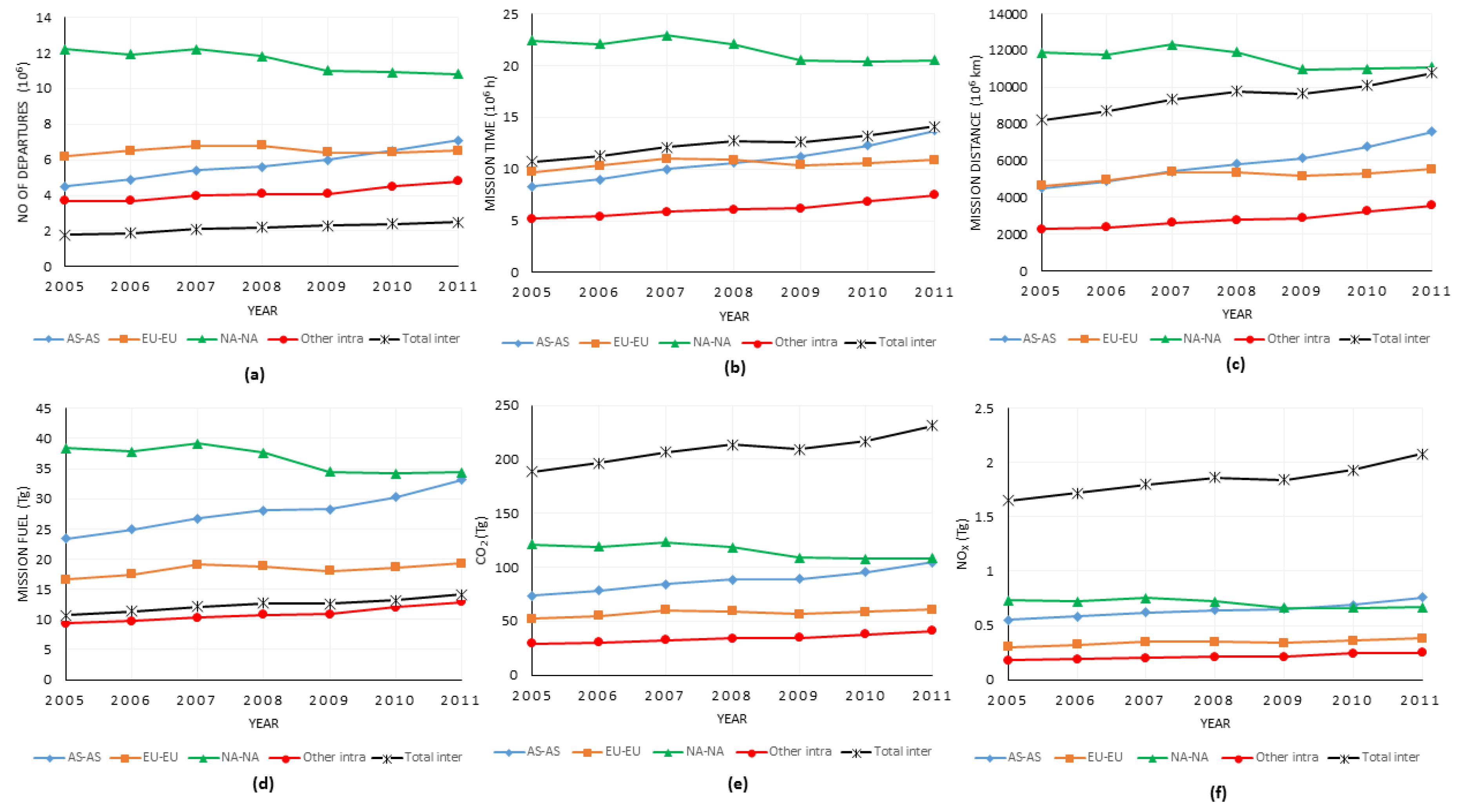
3.4. Regional Totals

Global air traffic, in terms of the number of departures, was dominated by intracontinental traffic within the regions of Asia (AS), Europe (EU), and North America (NA) which accounted for ~80% of the total each year between 2005 and 2011, resulting in ~50% and ~45% of the total global aircraft CO2 and NOx emissions, respectively (Figure 5). Historically NA is the world’s largest civil aviation market but by 2025, both EU (27%) and AS (32%) are predicted to have larger aviation markets than NA (25%) [45]. The regional results in the study show that in 2005, the AS and NA shares of the market (in terms of the number of departures) were 16% and 43%, respectively. By 2011, the respective shares were 22% and 34%, hence much closer to each other, with the AS share already bigger than the EU (21%) and rising, while the NA share is decreasing.
In 2005, there were 63% fewer departures, mission time and mission distance in AS than in NA, but the mission fuel, emissions of CO2, and NOx were only 39%, 40%, and 25% lower, respectively. By 2011, the number of departures, mission time, and mission distance in AS were 34%, 32%, and 33% lower than the number of departures, mission time, and mission distance in NA. However, mission fuel and CO2 emissions were only 3% and 4% lower in AS respectively, while the emissions of NOx were 13% higher. Considering the time period from 2005 to 2011, on average, there were 50% fewer departures (with 49% lower mission distance and 50% lower mission time) taking place within AS than in NA each year, but they were burning 34% less fuel and generating only 24% less CO2 and 8% less NOx each year (Figure 5).
Comparing AS with EU, there were 27% fewer departures and only 14 and 3% lower mission time and distance, respectively within AS than within EU in 2005, but the smaller number of intracontinental AS flights burned 41% more fuel and generated 40% more CO2 and 80% more NOx emissions than those within EU. By 2011, the number of the departures, mission time and distance in AS had overtaken the number of departures, mission time and distance in EU by 9%, 25%, and 37%, respectively and AS air traffic was generating 72% more CO2 emissions and 100% more NOx emissions by burning 72% more fuel than EU air traffic. On average for the time period of 2005-2011, there were 12% fewer departures, but 2% increased mission time and 13% increased mission distance within AS than within the EU each year, however they were generating 52% and 87% more CO2 and NOx per year (Figure 5). Comparing EU to NA, the results were more uniform. Between 2005 and 2011, on average, EU annual intracontinental departures, mission distance, mission time were 44%, 55%, and 51%, respectively lower than NA, but the mission fuel, CO2, and NOx annual emissions were also 50% lower within the EU than within NA (Figure 5).
The variabilities in the regional emission intensities of CO2 between AS, EU, NA during the time period of 2005–2011 suggest that AS air traffic is contributing more to aviation’s fraction of the total global CO2 burden. The regional and global atmospheric impact of the differences in the regional emissions intensities of aircraft NOx, in terms of increased tropospheric O3 production, is heterogeneous. Gilmore et al. [46] showed that the magnitude of sensitivity for southeast AS is a factor of 2 higher relative to NA for global O3 due to changes in regional NOx emissions. In this study, the annual average increase in the number of departures within AS was 8%, 1% in EU, and −1.9% in NA. Aviation is growing significantly faster in AS compared with EU and NA, so the emissions of NOx from aircraft grow at a higher rate and with a higher intensity in AS, which also has the strongest response in terms of O3 production to the addition of the NOx emissions.

4. Conclusions

On the 20th anniversary of the first comprehensive aircraft emission inventory, we presented a timeline of seven consecutive years (2005–2011) of estimates of the mission fuel burn, a reserve fuel requirement, and the emissions of CO2, CO, H2O, HC, NOx, and SOx of present day global and regional air traffic. The estimation referred to as the 4-D Aircraft Fuel Burn and Emissions Inventory was based on a detailed representation of the global fleet derived from actual records of air traffic movements and a detailed distribution of the fuel consumption and the emissions throughout the entire flight cycle. The 4-D Aircraft Fuel Burn and Emissions Inventory enabled a consistent global and regional trend analysis (2005–2011) and comparison of fuel burn and emissions for the first time since Kim et al. [27] who presented estimates for the time period 2000–2005, thus picking up the timeline in 2005, extending it to 2011, and bringing it up-to-date. An estimate of a global reserve fuel requirement was given for the first time within this work, which together with the mission fuel burn estimate provides an improved quantification of the global aviation fuel consumption with a fuel match of 1.1 (a 10% overestimate) relative to an IEA estimate for the total global jet kerosene production for 2009. The inventory results revealed that global estimates mask substantial regional fluctuations and differences in the quantity and distribution of the aircraft NOx emissions and in the number of departures, in particular, a persistent decline in North America and persistent growth in Asia. Moreover, a trend of substantially higher CO2 and NOx emission intensities within Asia is found if we compare their emissions within Europe and North America. A gradual shift in the global distribution of the NOx emissions from aircraft, and a subtle but steady change in the regional emission trends, are found with comparatively higher and rising growth rates in latitudes 0–30°N. These factors may have potentially large atmospheric implications in light of recent findings which indicate that the sensitivities to aircraft NOx emissions in Southeast Asia are more than double those in North America and Europe [46].

Supplementary Materials

The following are available online at https://www.mdpi.com/2073-4433/7/6/78/s1, Figure S1: Vertical distribution of the global aircraft CO2 emissions during 2005–2011; Figure S2: Vertical distribution of the global aircraft H2O emissions during 2005–2011; Figure S3: Vertical distribution of the global aircraft SOx emissions during 2005–2011.

Acknowledgements

We thank Stephen Roome (University of Bristol, IT support), Tom Gidden (http://www.linkedin.com/in/tomgidden), Matt Oates (University of Bristol, Bristol Centre for Complexity Sciences), Callum Wright (University of Bristol, Advanced Computing Research Centre), Sergio Angel Araujo Estrada (University of Bristol, Department of Aerospace Engineering), and Andy Williams for their support during the work. We also thank the Engineering and Physical Sciences Research Council (EPSRC) (grant EP/5011214) and the Natural Environmental Research Council (NERC) (grant-NE/J009008/1 and NE/I014381/1), University of Bristol Faculty of Engineering and School of Chemistry for funding various aspects of this work.

Author Contributions

D.K. Wasiuk, D.E. Shallcross, and M.H. Lowenberg conceived the idea, designed the experiments; D.K. Wasiuk and M.A.H. Khan analysed the data and wrote the paper; M.H. Lowenberg and D.E. Shallcross provided important suggestions and approved the final manuscript.

Conflicts of Interest

The authors declare no conflict of interest.

References

  1. Penner, J.E.; Lister, D.H.; Griggs, D.J.; Dokken, D.J.; McFarland, M. Aviation and the Global Atmosphere. A Special Report of Working Groups I and III of the Intergovernmental Panel on Climate Change (IPCC); Cambridge University Press: Cambridge, UK, 1999. [Google Scholar]
  2. Lee, D.S.; Pitari, G.; Grewe, V.; Gierens, K.; Penner, J.E.; Petzold, A.; Prather, M.J.; Schumann, U.; Bais, A.; Berntsen, T.; et al. Transport impacts on atmosphere and climate: Aviation. Atmos. Environ. 2010, 44, 4678–4734. [Google Scholar] [CrossRef]
  3. Lee, D.S.; Fahey, D.W.; Forster, P.M.; Newton, P.J.; Wit, R.C.N.; Lim, L.L.; Owen, B.; Sausen, R. Aviation and global climate change in the 21st century. Atmos. Environ. 2009, 43, 3520–3537. [Google Scholar] [CrossRef]
  4. Mahashabde, A.; Wolfe, P.; Ashok, A.; Dorbian, C.; He, Q.; Fan, A.; Lukachko, S.; Mozdzanowska, A.; Wollersheim, C.; Barrett, S.R.H.; et al. Assessing the environmental impacts of aircraft noise and emissions. Prog. Aero. Sci. 2011, 47, 15–52. [Google Scholar] [CrossRef]
  5. Holmes, C.D.; Tang, Q.; Prather, M.J. Uncertainties in climate assessment for the case of aviation NO. Proc. Natl Acad. Sci. USA 2011, 108, 10997–11002. [Google Scholar] [CrossRef] [PubMed]
  6. Burkhardt, U.; Kärcher, B. Global radiation forcing from contrail cirrus. Nat. Clim. Change 2011, 1, 54–58. [Google Scholar] [CrossRef]
  7. Skowron, A.; Lee, D.S.; de León, R.R. The assessment of the impact of aviation NOx on ozone and other radiative forcing responses: The importance of representing cruise altitudes accurately. Atmos. Environ. 2013, 74, 159–168. [Google Scholar] [CrossRef]
  8. Olsen, S.C.; Wuebbles, D.J.; Owen, B. Comparison of global 3-D aviation emissions datasets. Atmos. Chem. Phys. 2013, 13, 429–441. [Google Scholar] [CrossRef]
  9. Dessens, O.; Köhler, M.O.; Rogers, H.L.; Jones, R.L.; Pyle, J.A. Aviation and climate change. Transport. Policy 2014, 34, 14–20. [Google Scholar] [CrossRef]
  10. Brasseur, G.P.; Gupta, M.; Anderson, B.E.; Balasubramanian, S.; Barrett, S.; Duda, D.; Fleming, G.; Forster, P.M.; Fuglestvedt, J.; Gettelman, A.; et al. Impact of Aviation on Climate: FAA’s Aviation Climate Change Research Initiative (ACCRI) Phase II. Bull. Amer. Meteor. Soc. 2015. [Google Scholar] [CrossRef]
  11. Airbus. Global Market Forecast 2015–2034, 2015. Available online: http://www.airbus.com/company/market/forecast/ (accessed on 20 December 2015).
  12. European Commission Climate Action (ECCA), 2015. Available online: http://ec.europa.eu/clima/policies/transport/aviation/index_en.htm (accessed on 21 August 2015).
  13. Brasseur, G.P.; Cox, R.A.; Hauglustaine, D.; Isaksen, I.; Lelieveld, J.; Lister, D.H.; Sausen, R.; Schumann, U.; Wahner, A.; Wiesen, P. European scientific assessment of the atmospheric effects of aircraft emissions. Atmos. Environ. 1998, 32, 2329–2418. [Google Scholar] [CrossRef]
  14. Kentarchos, A.S.; Roelofs, G.J. Impact of aircraft NOx emissions on tropospheric ozone calculated with a chemistry general circulation model: sensitivity to higher hydrocarbon chemistry. J. Geophys. Res. 2002, 107, ACH 8-1–ACH 8-12. [Google Scholar] [CrossRef]
  15. Brühl, C.; Pöschl, U.; Crulzen, P.J.; Steil, B. Acetone and PAN in the upper troposphere: Impact on ozone production from aircraft emissions. Atmos. Environ. 2000, 34, 3931–3938. [Google Scholar] [CrossRef]
  16. Köhler, M.O.; Rädel, G.; Dessens, O.; Shine, K.P.; Rogers, H.L.; Wild, O.; Pyle, J.A. Impact of perturbations to nitrogen oxide emissions from global aviation. J. Geophys. Res. 2008, 113, D11305. [Google Scholar] [CrossRef]
  17. Grewe, V.; Stenke, A. AirClim: An efficient tool for climate evaluation of aircraft technology. Atmos. Chem. Phys. 2008, 8, 4621–4639. [Google Scholar] [CrossRef]
  18. Pitari, G.; Mancini, E.; Bregman, A. Climate forcing of subsonic aviation: Indirect role of sulfate particles via heterogeneous chemistry. Geophys. Res. Lett. 2002, 29, 2057. [Google Scholar] [CrossRef]
  19. McInnes, G.; Walker, C.T. The Global Distribution of Aircraft Air Pollutant Emissions; Warren Spring Laboratory Report LR872; Department of Trade and Industry, Warren Spring Laboratory: Stevenage, UK, 1992.
  20. Wuebbles, D.J.; Maiden, D.; Seals, R.K.; Baughcum, S.L.; Metwally, M.; Mortlock, A. Emissions scenarios development: Report of the emissions scenarios committee. In The Atmospheric Effects of Stratospheric Aircraft: A Third Program Report; Stolarski, R.S., Wesoky, H.L., Eds.; NASA Reference Publication 1313; National Aeronautics and Space Administration: Washington, DC, USA, 1993; pp. 63–85. [Google Scholar]
  21. ANCAT/EC. A Global Inventory of Aircraft NOx Emissions. A First Version (April 1994) Prepared for the AERONOX Programme; Abatement of Nuisances Caused by Air Transport (ANCAT) and European Community Working Group: London, UK, 1995. [Google Scholar]
  22. Baughcum, S.L.; Henderson, S.C.; Hertel, P.S.; Maggiora, D.R.; Oncina, C.A. Stratospheric Emissions Effects Database Development; Boeing Commercial Airplane Group, National Aeronautics and Space Administration (NASA) Contractor Report 4592; Langley Research Centre: Hampton, VA, USA, 1994.
  23. Baughcum, S.L.; Henderson, S.C.; Tritz, T.G. Scheduled Civil Aircraft Emission Inventories for 1976 and 1984: Database Development and Analysis; Boeing Commercial Airplane Group, National Aeronautics and Space Administration (NASA) Contractor Report-4722; Langley Research Centre: Hampton, VA, USA, 1996.
  24. Baughcum, S.L.; Tritz, T.G.; Henderson, S.C.; Pickett, D.C. Scheduled Civil Aircraft Emission Inventories for 1992: Database Development and Analysis; National Aeronautics and Space Administration Contractor Report-4700; Langley Research Centre: Hampton, VA, USA, 1996.
  25. Sutkus, D.J., Jr.; Baughcum, S.L.; DuBois, D.P. Commercial Aircraft Emission Scenario for 2020: Database Development and Analysis; NASA/CR-2003-212331; National Aeronautics and Space Administration, Glenn Research Centre: Hanover, MD, USA, 2003.
  26. Eyers, C.J.; Norman, P.; Middel, J.; Plohr, M.; Michot, S.; Atkinson, K. AERO2k Global Aviation Emissions Inventories for 2002 and 2025; European Commission, QinetiQ Ltd.: Hampshire, UK, 2004. [Google Scholar]
  27. Gardner, R.M.; Adams, K.; Cook, T.; Deidewig, F.; Ernedal, S.; Falk, R.; Fleuti, E.; Herms, E.; Johnson, C.E.; Lecht, M.; et al. The ANCAT/EC global inventory of NOx emissions from aircraft. Atmos. Environ. 1997, 31, 1751–1766. [Google Scholar] [CrossRef]
  28. Kim, B.Y.; Fleming, G.; Balasubramanian, S.; Malwitz, A.; Lee, J.; Waitz, I.; Klima, K.; Locke, M.; Holsclaw, C.; Morales, A.; McQueen, E.; Gillette, W. System for Assessing Aviation’s Global Emissions (SAGE), Version 1.5; Global Aviation Emissions Inventories for 2000 through 2004; FAA-EE-2005–02; Federal Aviation Administration Office of Environment and Energy: Washington, DC, USA, 2005. [Google Scholar]
  29. Kim, B.Y.; Fleming, G.G.; Lee, J.J.; Waitz, I.A.; Clarke, J.P.; Balasubramanian, S.; Malwitz, A.; Klima, K.; Locke, M.; Holslaw, C.A.; et al. System for assessing Aviation’s Global Emissions (SAGE), Part 1: Model description and inventory results. Transport. Res. Part D: Transp. Environ. 2007, 12, 325–346. [Google Scholar] [CrossRef]
  30. Wilkerson, J.T.; Jacobson, M.Z.; Malwitz, A.; Balasubramanian, S.; Wayson, R.; Fleming, G.; Naiman, A.D.; Lele, S.K. Analysis of emission data from global commercial aviation: 2004 and 2006. Atmos. Chem. Phys. 2010, 10, 6391–6408. [Google Scholar] [CrossRef]
  31. Owen, B.; Lee, D.S.; Lim, L. Flying into the future: aviation emissions scenarios to 2050. Environ. Sci. Technol. 2010, 44, 2255–2260. [Google Scholar] [CrossRef] [PubMed]
  32. Chèze, B.; Gastineau, P.; Chevallier, J. Forecasting world and regional aviation jet fuel demands to the mid-term (2025). Energy Policy 2011, 39, 5147–5158. [Google Scholar] [CrossRef]
  33. Simone, N.W.; Stettler, M.E.J.; Barrett, S.R.H. Rapid estimation of global civil aviation emissions with uncertainty quantification. Transport. Res. Part D Transp. Environ. 2013, 25, 33–41. [Google Scholar] [CrossRef]
  34. Yan, F.; Winijkul, E.; Streets, D.G.; Lu, Z.; Bond, T.C.; Zhang, Y. Global emission projections for the transportation sector using dynamic technology modelling. Atmos. Chem. Phys. 2014, 14, 5709–5733. [Google Scholar] [CrossRef]
  35. Wasiuk, D.K.; Lowenberg, M.H.; Shallcross, D.E. An aircraft performance model implementation for the estimation of global and regional commercial aviation fuel burn and emissions. Transport. Res. Part D Transp. Environ. 2015, 35, 142–159. [Google Scholar] [CrossRef]
  36. ICAO. Aircraft Engine Emissions Databank, 18th ed.; International Civil Aviation Organization Committee on Aviation Environmental Protection: Montreal, YQB, Canada, 2012. [Google Scholar]
  37. Hasselrot, A. Confidential Database for Turboprop Engine Emissions; Swedish Defence Research Agency: Stockholm, Sweden, 2002.
  38. DuBois, D.; Paynter, G.C. Fuel Flow Method 2 for Estimating Aircraft Emissions; SAElnternational, The Boing Company: Washington, DC, USA, 2006. [Google Scholar]
  39. SAE. SAE Aerospace. Procedure for the Calculation of Aircraft Emissions; Technical Report AIR5715; SAE International: Warrendale, PA, USA, 2009. [Google Scholar]
  40. Collins, W.J.; Stevenson, D.S.; Johnson, C.E.; Derwent, R.G. Tropospheric ozone in a Global-Scale Three-Dimensional Lagrangian Model and its response to NOx emission controls. J. Atmos. Chem. 1997, 26, 223–274. [Google Scholar] [CrossRef]
  41. Utembe, S.R.; Cooke, M.C.; Archibald, A.T.; Jenkin, M.E.; Derwent, R.G.; Shallcross, D.E. Using a reduced Common Representative Intermediates (CRI v2-R5) mechanism to simulate tropospheric ozone in a 3-D Lagrangian chemistry transport model. Atmos. Environ. 2010, 13, 1609–1622. [Google Scholar] [CrossRef]
  42. Schumann, U. The impact of nitrogen oxides emissions from aircraft upon the atmosphere at flight altitudes–results from the AERONOX project. Atmos. Environ. 1997, 31, 1723–1733. [Google Scholar] [CrossRef]
  43. IEA. International Energy Agency Oil Statistics. 2015. Available online: http://www.iea.org/stats/oildata.asp?COUNTRY_CODE=29 (accessed on 06 May 2015).
  44. Sutkus, D.J., Jr.; Baughcum, S.L.; DuBois, D.P. Scheduled Civil Aircraft Emission Inventories for 1999: Database Development and Analysis; NASA/CR-2001-211216; National Aeronautics and Space Administration, Glenn Research Centre: Hanover, MD, USA, 2001.
  45. Belobaba, P.; Odoni, A.; Barnhart, C. The Global Airline Industry, 2nd ed.; John Wiley & Sons, Ltd.: West Sussex, UK, 2015. [Google Scholar]
  46. Gilmore, C.K.; Barrett, S.R.H.; Koo, J.; Wang, Q. Temporal and spatial variability in the aviation NOx-related O3 impact. Environ. Res. Lett. 2013, 8, 034027. [Google Scholar] [CrossRef]
Figure 1. NOx emissions trajectory on the STOCHEM grid. TOUT stands for taxi out, CL for climb, CR for cruise, DES for descent, TIN for taxi in, p for the number of grids that the path from A to B spans and n for the number of levels.
Atmosphere 07 00078 g001
Figure 2. Vertical distribution of the global total (a) mission fuel burn, (b) mission time, (c) mission distance, (d) CO emissions, (e) HC emissions, and (f) NOx emissions during 2005–2011.
Atmosphere 07 00078 g002
Figure 3. The average (2005–2011) distribution of the global aircraft NOx emissions (in Tg), (a) between 5.6 and 7.2 km, (b) between 7.2 and 9.2 km, (c) between 9.2 and 11.8 km, (d) between 11.8 and 16.2 km.
Atmosphere 07 00078 g003
Figure 4. The fraction (%) of the total global annual emissions of aircraft NOx allocated to the NH in each 10° latitude band from 0°N to 90°N for the period of 2005–2011.
Atmosphere 07 00078 g004
Figure 5. Regional totals of (a) the number of departures, (b) mission time, (c) mission distance, (d) mission fuel, (e) CO2 emissions, (f) NOx emissions for 2005–2011. Note: Other intra consists of AF↔AF, CA↔CA, CB↔CB, ME↔ME, SA↔SA, SW↔SW. AS, EU, NA, AF, CA, CB, ME, SA, SW represent Asia, Europe, North America, Africa, Central America, Caribbean, Middle East, South America, Australasia, respectively.
Atmosphere 07 00078 g005
Table 1. Global totals and percent changes of the number of departures, mission distance and time, total fuel, mission fuel, and reserve fuel during 2005–2011.
Year2005200620072008200920102011
Departures (106)28.428.930.5 30.629.7 30.731.8
(1.9)(5.6)(0.2)(−2.8)(3.2)(3.8)
Distance (109 km)31.532.735.035.634.836.438.5
(3.8)(7.2)(1.7)(−2.4)(4.5)(5.9)
Mission time (106 h)56.358.061.962.660.963.466.7
(3.1)(6.6)(1.1)(−2.6)(4.0)(5.2)
Mission fuel burn (Tg)147.6152.2160.9163.0158.1163.9173.2
(3.1)(5.7)(1.3)(−3.0)(3.6)(5.7)
Reserve fuel (Tg)94.096.0101.6102.199.0102.0106.4
(2.1)(5.8)(0.6)(−3.1)(3.0)(4.3)
Note: The percentage annual changes are shown in parenthesis.
Table 2. Global annual fuel burn and aircraft CO2, CO, H2O, HC, NOx and SOx emissions in this study and their comparison with previous inventories.
YearFuel Burn (Tg)CO2 (Tg)CO (Tg)H2O (Tg)HC (Tg)NOx (Tg)SOx (Tg)Reference
199092.8293.00.53115.00.141.20.074[22]
1992110.0347.0n/a135.0n/an/a0.13[8]
199294.9423.00.50165.00.1951.2n/a[24]
1999128.0n/a0.69n/a0.191.7n/a[44]
1999136.0430.00.67167.00.231.40.16[8]
2000181.0572.00.54224.00.082.50.15[28]
2000214.0677.0n/an/an/a2.9n/a[31]
2000152.0480.0n/a187.0n/a2.00.18[8]
2001170.0536.00.46210.00.062.40.14[28]
2002171.0539.00.48211.00.062.40.14[28]
2002156.0492.00.51193.00.062.1n/a[26]
2002154.0486.0n/a190.0n/an/a0.18[8]
2003176.0557.00.49218.00.062.50.14[28]
2004188.0595.00.51233.00.062.70.15[28]
2004174.1549.70.63215.30.092.50.20[30]
2005203.0641.00.55251.00.072.90.16[29]
2005180.6570.50.75n/a0.22.70.22[33]
2005147.6464.70.78181.50.283.40.12This study
2006188.2594.30.68232.80.102.70.22[8,30]
2006152.2479.30.74187.20.243.50.13This study
2007160.9506.80.75198.00.233.70.14This study
2008229.0725.00.69282.00.093.20.18[32]
2008163.0513.40.74200.50.213.80.14This study
2009158.1498.00.69194.50.183.70.13This study
2010240.0n/a1.92n/a0.33.02n/a[34]
2010163.9516.00.69201.50.173.90.14This study
2011173.2545.30.70213.00.164.10.15This study
2015255.0803.01.14315.00.102.30.10[22]
2015282.0n/a1.44n/a0.233.9n/a[25]
2020336.0n/a1.39n/a0.234.9n/a[25]
2025327.01029.01.15404.00.153.3n/a[26]
2030440.0n/a2.33n/a0.294.95n/a[34]
2050770.0n/a2.64n/a0.257.5n/a[34]
Notes: n/a denotes no available data; NOx (Tg) and SOx (Tg) are reported as NO2 (Tg) and SO2 (Tg), respectively.

