Accurate Characterization of Winter Precipitation Using Multi-Angle Snowflake Camera, Visual Hull, Advanced Scattering Methods and Polarimetric Radar

Abstract

This article proposes and presents a novel approach to the characterization of winter precipitation and modeling of radar observables through a synergistic use of advanced optical disdrometers for microphysical and geometrical measurements of ice and snow particles (in particular, a multi-angle snowflake camera—MASC), image processing methodology, advanced method-of-moments scattering computations, and state-of-the-art polarimetric radars. The article also describes the newly built and established MASCRAD (MASC + Radar) in-situ measurement site, under the umbrella of CSU-CHILL Radar, as well as the MASCRAD project and 2014/2015 winter campaign. We apply a visual hull method to reconstruct 3D shapes of ice particles based on high-resolution MASC images, and perform “particle-by-particle” scattering computations to obtain polarimetric radar observables. The article also presents and discusses selected illustrative observation data, results, and analyses for three cases with widely-differing meteorological settings that involve contrasting hydrometeor forms. Illustrative results of scattering calculations based on MASC images captured during these events, in comparison with radar data, as well as selected comparative studies of snow habits from MASC, 2D video-disdrometer, and CHILL radar data, are presented, along with the analysis of microphysical characteristics of particles. In the longer term, this work has potential to significantly improve the radar-based quantitative winter-precipitation estimation.

1. Introduction

Winter precipitation can, in extreme conditions, cause substantial damage and havoc, as in the case of ice storms or heavy snow storms; such storms are also of considerable impact on aviation safety. The literature on the microphysics of winter precipitation, which is characterized by a large variety of ice particles, is rather rich, with great efforts being expended into modeling, in-situ measurements, and remote sensing of the particles [1,2]. Here, we focus on in-situ measurements of hydrometeor characteristics such as fall speed, size, shape, and density, development of physical and scattering models of natural snow and ice particles, computation of realistic particle scattering matrices and full polarimetric variables, and dual-polarized radar observations. Our overarching long-term goal is the improvement of radar-based methods of classification of hydrometeor types and estimation of the liquid equivalent snow rates.

Straka et al. [3] have summarized the key microphysical characteristics of ice crystals and aggregates, as well as the corresponding ranges of dual-polarized radar observables useful for type classification. One limiting factor is the large uncertainty in going from idealized microphysical characteristics of ice hydrometeors to the appropriate scattering model and hence to calculation of the scattering matrix. For example, the particle density (which often depends on particle size, especially for snow aggregates) plays an important role in determining the scattering matrix but can cause large errors if the wrong density is assumed [4,5]. Similarly, assuming idealized spheroidal shapes for ice particles instead of the more complicated realistic three-dimensional (3D) shapes can also cause errors in the scattering matrix [6]. Some radar signatures assuming spheroidal shapes for plate or column-like crystals have been successful in showing consistency with radar measurements [4,7,8,9,10]. In general, however, it is very difficult to explain all of the polarimetric radar measurables, namely, horizontal reflectivity, Z_h, differential reflectivity, Z_dr, linear depolarization ratio, LDR, specific differential phase, K_dp, and co-polar correlation coefficient, ρ_hv, in winter precipitation simultaneously using spheroidal shape models with specified densities and orientation distributions. In fact, it is in the computation of the reflectivity Z_e that simple scattering models, and dielectric constant based on the average density versus apparent diameter (D_app) power law relationship are invoked. However, even for Rayleigh scattering, where the spherical or spheroidal shape assumption is reasonable for Z_e computation [11], it is not sufficient for computing the full scattering matrix and related radar measurables (Z_dr, LDR, and ρ_hv), required for radar-based particle classification. So, even at the S-band (all WSR-88D radars), Z_dr, LDR, and ρ_hv significantly depend on the shape and composition of particles, and even at 3 GHz, sophisticated scattering methods are needed for radar parameters other than Z_e.

The estimation of liquid equivalent snow rate (henceforth snow rate or SR) from radar measurements has long been recognized as a difficult problem in quantitative precipitation estimation (QPE), but one of great importance given the large areal coverage afforded by the WSR-88D network. With the advent of optical imaging disdrometers that can measure fall speed along with projected particle views in either one plane (hydrometeor velocity and shape detector (HVSD) [12]) or two planes (2D-video disdrometer [13]), and well-calibrated radars, there appears to be progress made in QPE [14,15,16]. In essence, the measure of the fall speed and “area”-ratio (along with state parameters) permits estimation of the particle mass [17,18]. The apparent volume of the particle is estimated from the image (more accurately from two orthogonal views as with the 2DVD), and an average density—D_app power law is derived. With the measure of the particle size distribution (PSD), where “size” refers to D_app, the snow accumulation is estimated and compared with collocated snow gauge. These latter “microphysical” steps can be accomplished with a single 2DVD (or with HVSD) and validated with an accurate snow gauge (such as Geonor or Pluvio). Huang et al. [15] derived Z_e–SR power law for specific winter precipitation events, and then applied it to radar observations to produce a radar-based snow accumulation map, with these accumulations being compared to accumulations from other gauges under the radar umbrella. However, the current operational version of cool season precipitation-type classification performs poorly, while the quantification of liquid equivalent SR is generally based on climatological Z_e–SR power laws which can give large errors with respect to gauge measurements (not surprising given the large variability in snow microphysics).

Straka et al. [3] and Zrnić et al. [19] proposed that QPE in general could be improved by first classifying particle types with polarimetric radar prior to quantification. For example, the WSR-88D operational estimation of rainfall is achieved by polarimetric-based classification followed by quantification using Z_h, Z_dr, and K_dp in rain-only regions and empirical Z–R power laws when other types of hydrometeors, such as wet snow, graupel, dry snow or crystals, are identified at long ranges where the beam overshoots the freezing level [20].

In terms of scattering models and techniques, the T-matrix method [21] and the discrete dipole approximation (DDA) method [22] are the two conventionally and almost exclusively used tools in atmospheric particle scattering analysis. The T-matrix method is extremely fast. However, most of the working T-matrix tools are able to calculate scattering properties of rotationally symmetric particles only, and only those with smooth surfaces. The major advantage of the DDA method is that it can be applied to arbitrarily shaped particles. However, the numerical accuracy of the method is relatively low, and improves slowly with increasing the number of dipoles, which makes the DDA computation very time-consuming. In addition, the DDA codes do not converge for any reasonable predefined accuracy and number of iteration steps in some cases with high-contrast dielectric materials and large electrical sizes of particles. The T-matrix solution does not converge or exhibits an erratic behavior in some cases with electrically large or geometrically complex particles, namely, those with a large aspect ratio.

Overall, shape and composition (density) of ice and snow particles have a significant impact on radar observations, and current physical and scattering models, and thus radar-based precipitation retrievals, do not take this into account adequately.

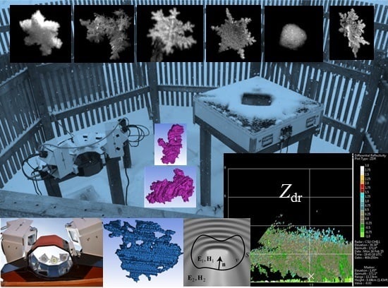
This article proposes and presents a novel approach to characterization of winter precipitation and modeling of radar observables through a synergistic use of advanced optical imaging disdrometers for microphysical and geometrical measurements of ice and snow particles, image processing methodology to reconstruct complex particle 3D shapes, full-wave computational electromagnetics (CEM) to analyze realistic winter precipitation scattering, and state-of-the-art polarimetric radar to validate the modeling approach. The principal enabling methodologies and technologies are specifically (i) multi-angle snowflake camera (MASC) and two-dimensional video disdrometer (2DVD); (ii) visual hull geometrical method for reconstruction of 3D hydrometeor shapes; (iii) efficient and accurate CEM scattering models and solutions based on a higher order method of moments (MoM) in the surface integral equation (SIE) formulation and the frequency domain; and (iv) fully polarimetric data from the Colorado State University (CSU) CHILL radar, with added observations from the National Center for Atmospheric Research (NCAR) SPOL radar [23,24,25,26,27]. We develop physical and scattering models of natural snowflakes using the MASC, 2DVD, visual hull, and advanced scattering methods, with the modeling and scattering calculations being verified and validated by CSU-CHILL and SPOL radar observations. We also perform comparative studies of snow habits from MASC, 2DVD, and CHILL radar data and analyze microphysical characteristics of particles.

A modified MASC system, within a double wind fence, is used to capture five different high-resolution images of an ice particle in free-fall. We apply the visual hull method to reconstruct 3D shapes of particles based on these images. We use the fall-speed from the MASC and the collocated 2DVD, along with measured state parameters, to estimate the dielectric constant of particles. By calculation of “particle-by-particle” scattering matrices based on the reconstructed shapes and estimated dielectric constant, we obtain polarimetric radar observables.

Overall, the main goal of this article is to propose the synergistic use of new research instrumentation (MASC) coupled with accurate and fast CEM scattering computation as well as state-of-the-art polarimetric radar (with exceptional polarization purity) and other in-situ surface instrumentation to substantially increase the accuracy of modeling of radar observables and characterization of winter precipitation, including comparative studies of snow habits and analyses of microphysical characteristics of particles. The goal of the article is also to describe the newly built and established MASCRAD (MASC + Radar) in-situ measurement site, in the proximity of CSU-CHILL Radar, near Greeley, Colorado. The goal as well is to describe the MASCRAD project and the 2014/2015 MASCRAD winter campaign, along with illustrative results and analyses. The article presents and discusses selected illustrative data collected during several 2014/2015 MASCRAD cases with widely-differing meteorological settings that involved contrasting hydrometeor forms [28,29,30]. Of particular interest were episodes when the occurrence of vertically-oriented graupel, pristine individual ice crystals, and large-diameter aggregates were observed. Also shown are illustrative results of scattering calculations based on MASC images captured during these events, in comparison with radar data, as well as microphysical characteristics analysis of some cases.

The MASCRAD surface instrumentation field site includes a 2/3-scaled double fence intercomparison reference (DFIR) wind shield housing MASC, 2DVD, PLUVIO snow measuring gauge, VAISALA weather station, as well as the collocated NCAR GPS advanced upper-air system sounding system trailer, under the umbrella of two state-of-the-art polarimetric weather radars, CSU-CHILL Radar and NCAR SPOL Radar, with high spatial and temporal resolutions and special scan strategies. It is supported by excellent geometrical and image processing and scattering modeling and computing capabilities, and is one of the currently best instrumented and most sophisticated field sites for winter precipitation measurements and analysis worldwide. This is the first time real (measured) snowflake images have been used with reconstructions of 3D hydrometeor shapes and realistic scattering calculations, to obtain radar measurable parameters, which are then compared and analyzed against measurements by highly precise polarimetric radars.

In a longer term, this work has potential to significantly improve the radar-based QPE and estimation of liquid equivalent snow rates near the surface in stronger, more hazardous, winter events by first classification of precipitation type followed by quantification. Overall, there is great need and interest for advances in characterization, classification, and quantification of snow—largely an unsolved, extremely important, problem.

Specifically, there has been great and increasing interest by meteorologists and atmospheric scientists in microphysical properties of winter precipitation, where new discoveries are anticipated and the synergy between polarimetric radar observations, optical measurements and processing, and advanced electromagnetic scattering computations is expected to bring significant advancements. In addition, as snow is currently the least understood component of the global water cycle, the importance of studies on parametrization of snow and ice particle microphysics in numerical weather prediction models can hardly be overstated.

2. Capturing Snowflake Images in Freefall by Multi-Angle Snowflake Camera

The multi-angle snowflake camera (MASC), shown in Figure 1a, is a new instrument for capturing high-resolution photographs of snow and ice particles in freefall from three views, while simultaneously measuring their fall speed [31]. In the MASC system, the horizontal resolution is between 10 μm and 37 μm for different cameras and the vertical resolution at 1-m/s fall speed is 40 μm. For Colorado State University’s customized system, the horizontal resolution is 35.9 μm for the 3 original cameras and 89.6 μm for the 2 externally added cameras. The virtual measurement area is 30 cm² (about 1/3 of that of the 2DVD). Note that the horizontal resolution of the 2DVD for the current production model is around 160–170 μm, depends on the unit, which is not sufficient to resolve details of the complexity of ice particles in winter precipitation. There is, of course, a distinct advantage in obtaining photographs relative to the 2DVD contours to facilitate, for example, estimates of the degree of riming of snow particles.

Figure 1b shows the 3D schematic of the MASC, which consists of three cameras, with angular separation of 36° and the camera-to-common focal center distance of 10 cm. The near-IR emitter-detector pairs are separated vertically by 32 mm. Particles that fall through the lower array simultaneously trigger each of the three cameras and the bank of LEDs at a maximum triggering rate of 2 Hz. Fall speed is calculated from the time taken to traverse the distance between the upper and lower triggering arrays. While the standard version of the MASC uses cameras with different lenses, giving different horizontal field of views (FOVs), depth of fields (DOFs), and image resolutions [31] (Table 1), the CSU version has three identical cameras (5 MP (Megapixel) Unibrain Fire-i 980b digital cameras), with identical lenses (Fujinon 12.5 mm). The choice of 12.5-mm lenses not only gives a better match between the horizontal resolution and the motion blur length of ~40 μm, but it also means that particles are in-focus within the measurement area. 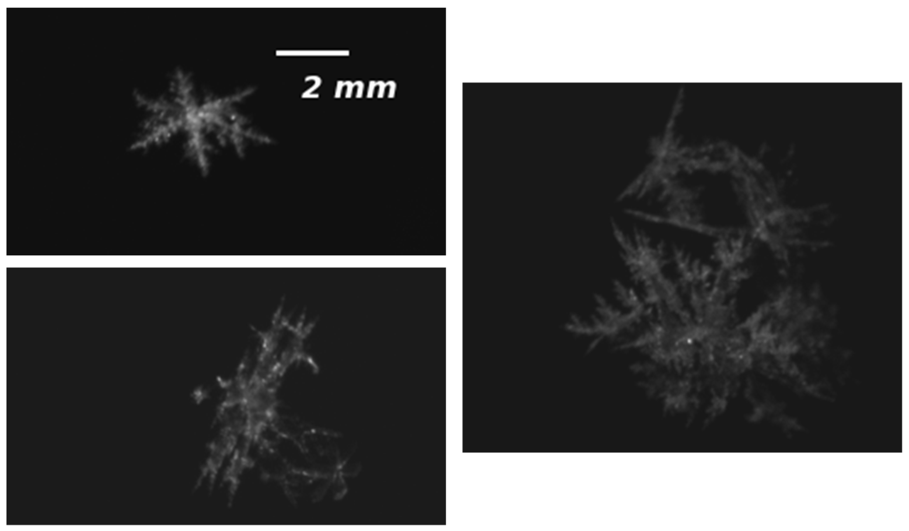Figure 1c gives a planar view for the prototype design for which the horizontal FOVs and DOFs are the same for the three cameras/lenses, and, more importantly, the virtual measurement area is precisely defined by the yellow-colored area, shown in Figure 1d. The only compromise with respect to the original design is that the horizontal resolution is degraded to 35.9 μm, at the center of the measurement area, which, however, is sufficient to get high-quality pictures of snow particles. 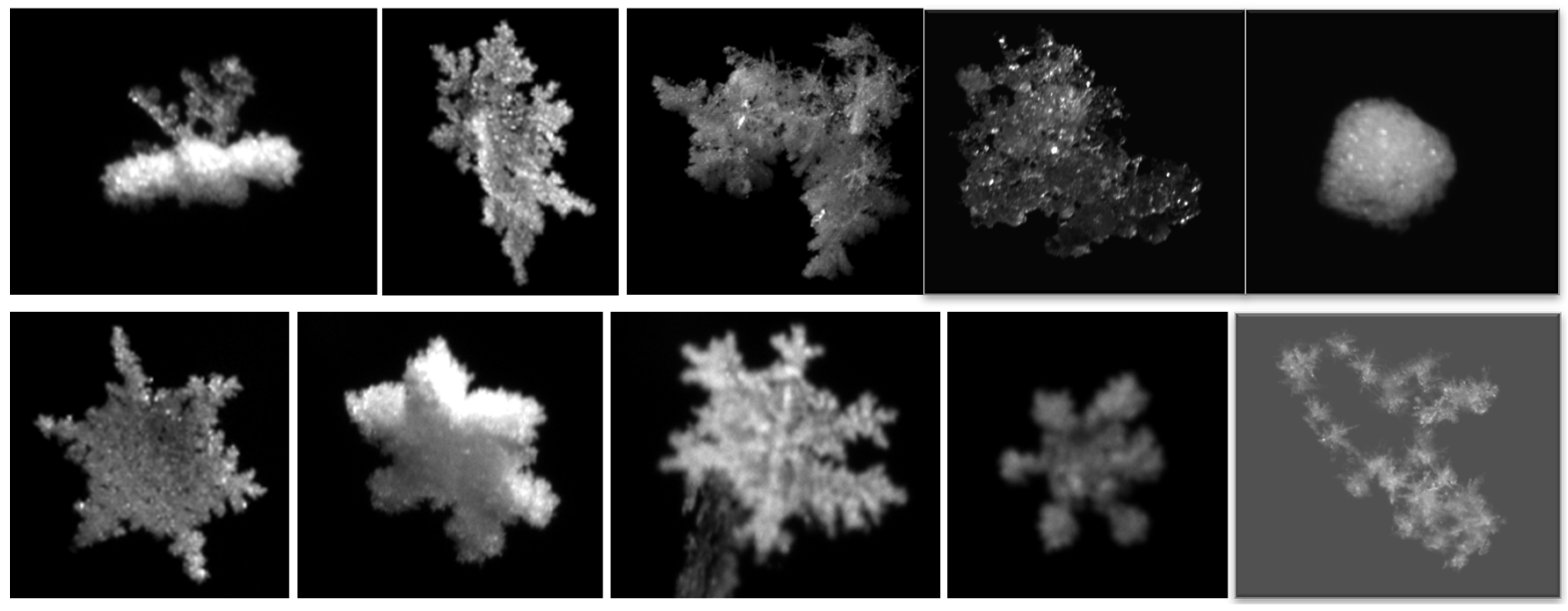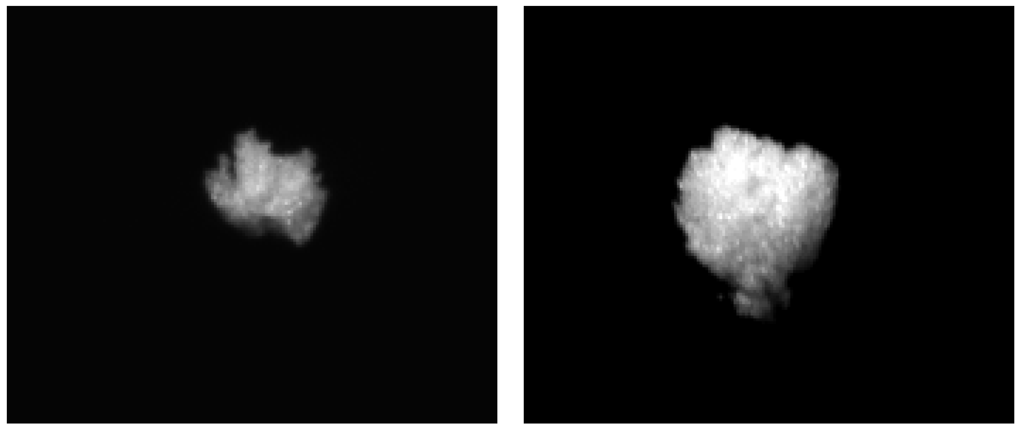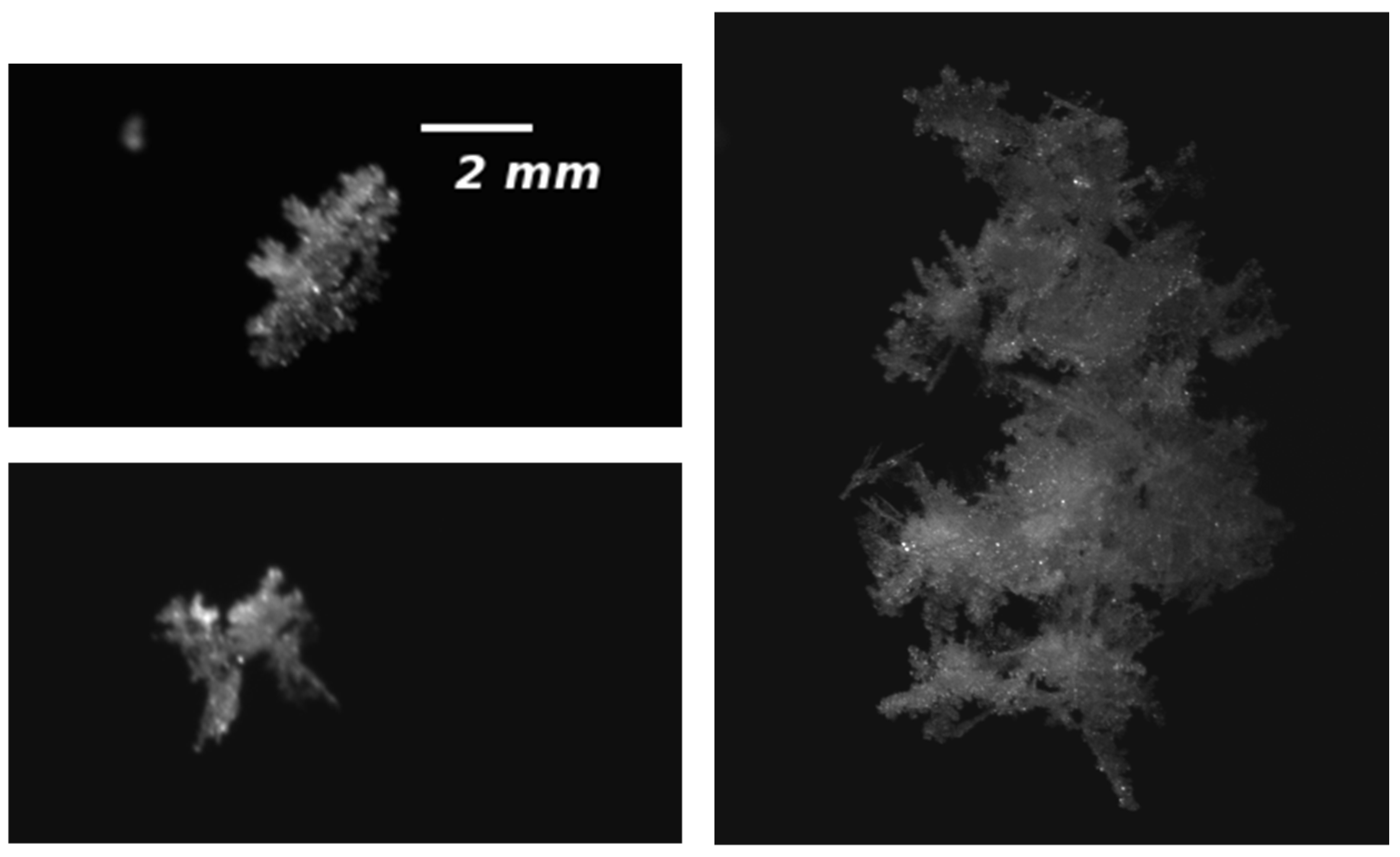Shown in Figure 2 are examples of MASC snowflake images collected at the MASCRAD Field Site.

We have developed a new mechanical calibration method for the MASC which significantly improves upon that currently used by the MASC manufacturer. In addition, we have also developed a multi-camera software self-calibration procedure to obtain a correction matrix for the MASC, based on the method by Svoboda et al. [32], which is the first software correction and compensation of a non-perfect mechanical calibration of the instrument. While this is still work in progress, our analysis methods and codes are generally able to handle and process MASC images with multiple snowflakes per image, which is a very significant advancement of the previously available analysis techniques.

3. Visual Hull Reconstruction of 3D Hydrometeor Shapes from MASC Images

We use the visual hull geometrical method and software to reconstruct 3D shapes of snow particles and other hydrometeors based on photographs obtained by the MASC (Figure 2), and the corresponding 2D silhouettes of an object [25,26]. Such a reconstruction enables realistic computation of “particle-by-particle” scattering matrices and simulation of radar observables. The visual hull of an object can be interpreted as the maximal domain that is silhouette-equivalent to the object, namely, that gives the same silhouettes as the object from a set of viewpoints (theoretically, from any viewpoint) [33,34,35,36]. The visual hull is obtained as an intersection of visual solid cones (five cones in our case) formed by back-projecting, from the viewpoints, the previously found silhouettes in the corresponding image planes situated in front of the (five) cameras, as illustrated in Figure 3. 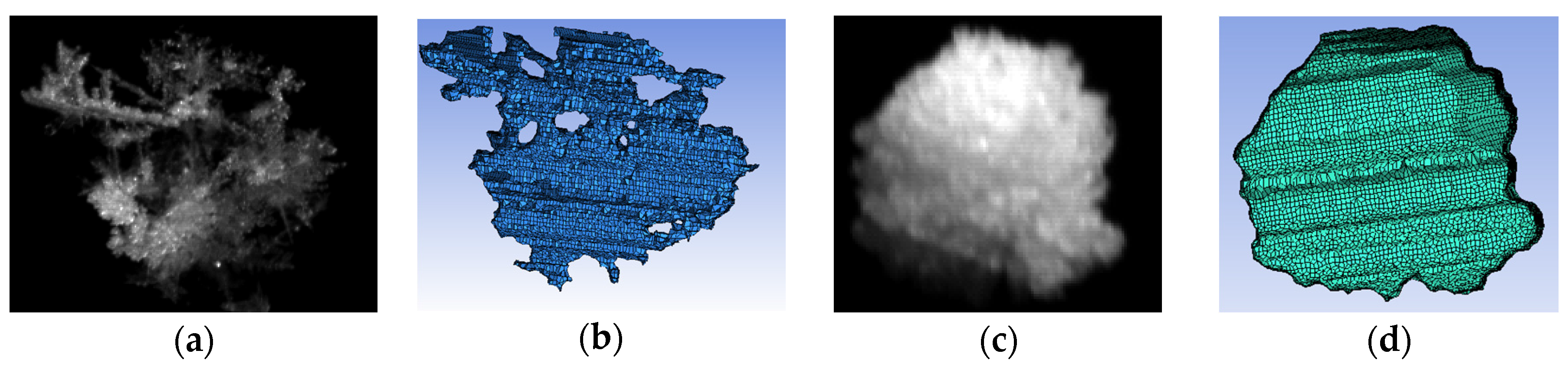In particular, we use an open-source MATLAB, C++ Visual Hull Mesh Code (VHMC) [37,38], that generates a visual hull mesh from silhouette images and associated camera parameters. Camera calibration and the corresponding information, such as focal lengths, lens distortion parameters, 3 × 3 rotation matrices, and 3 × 1 translation vectors, are essential for the accuracy of the VHMC shape reconstruction. In the code, the boundaries of silhouettes are approximated by polygons, and the final 3D model is represented by a mesh of flat triangular patches.

We are also able to compute readily, within the visual hull method and code, the volume of the 3D reconstructed particle, thus obtaining the volume estimation for hydrometeors. Along with the estimation of the particle mass using the theory of Böhm [17], this gives us the effective density (or porosity) of snowflakes, from which we are able to obtain the effective dielectric constant of the particle, which takes into account air inclusions and partly melted regions of ice crystals. Note, however, that the MASC/VHMC can capture some of the porosity of ice particles along with their complex shapes. In addition, we can easily compute, from the 3D particle reconstruction, the particle projected area presented to the flow that is necessary for Böhm’s method. Finally, the realistically and accurately (as much as possible) reconstructed 3D particle shapes can further be used for studies of snow habits, for advanced analyses of microphysical characteristics of particles, and for particle classifications.

Figure 3 shows an example of snowflake reconstruction by the VHMC based on three MASC (Figure 1) photographs of a snowflake. We observe very good results, which are much better than any snowflake 3D realistic-shape reconstruction data in the literature, e.g., [31,39,40,41], and are indicative of the potential of the MASC-VHMC approach, coupled with advanced CEM scattering methods and codes, as well as advanced and emerging approaches to studies of snow habits, microphysical characteristics analysis, hydrometeor classification, 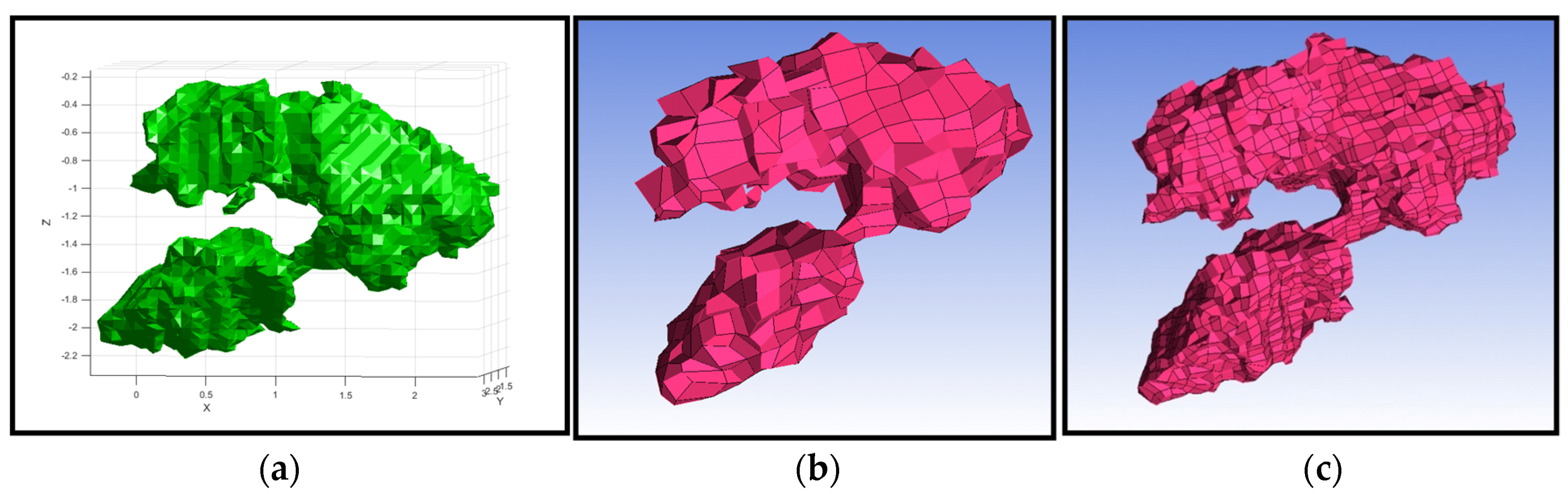etc.

However, 3D reconstructed snowflakes from the three MASC photographs are, generally, not close enough to the real shapes of the snowflakes. This is because of the insufficient information from the three MASC cameras being placed at 36° with respect to each other in one plane, as can be seen in Figure 1c, covering only 72° in front of the object (MASC is not intended for 3D shape reconstruction). In order to improve the 3D reconstruction obtained from the visual hull method, two additional cameras are added to the MASC, “externally”, to provide additional views. They are on an elevated plane with respect to the original three, at about a 55° angle above horizon, as shown in Figure 1e,f. All five cameras trigger simultaneously and collect images at a 2-Hz rate. We perform 5-camera software self-calibration of the MASC, to obtain a correction matrix that is then used as an input to the visual hull code to correct for a non-perfect mechanical calibration. Without this, the visual hull fails to create 3D reconstructions for many snowflakes.

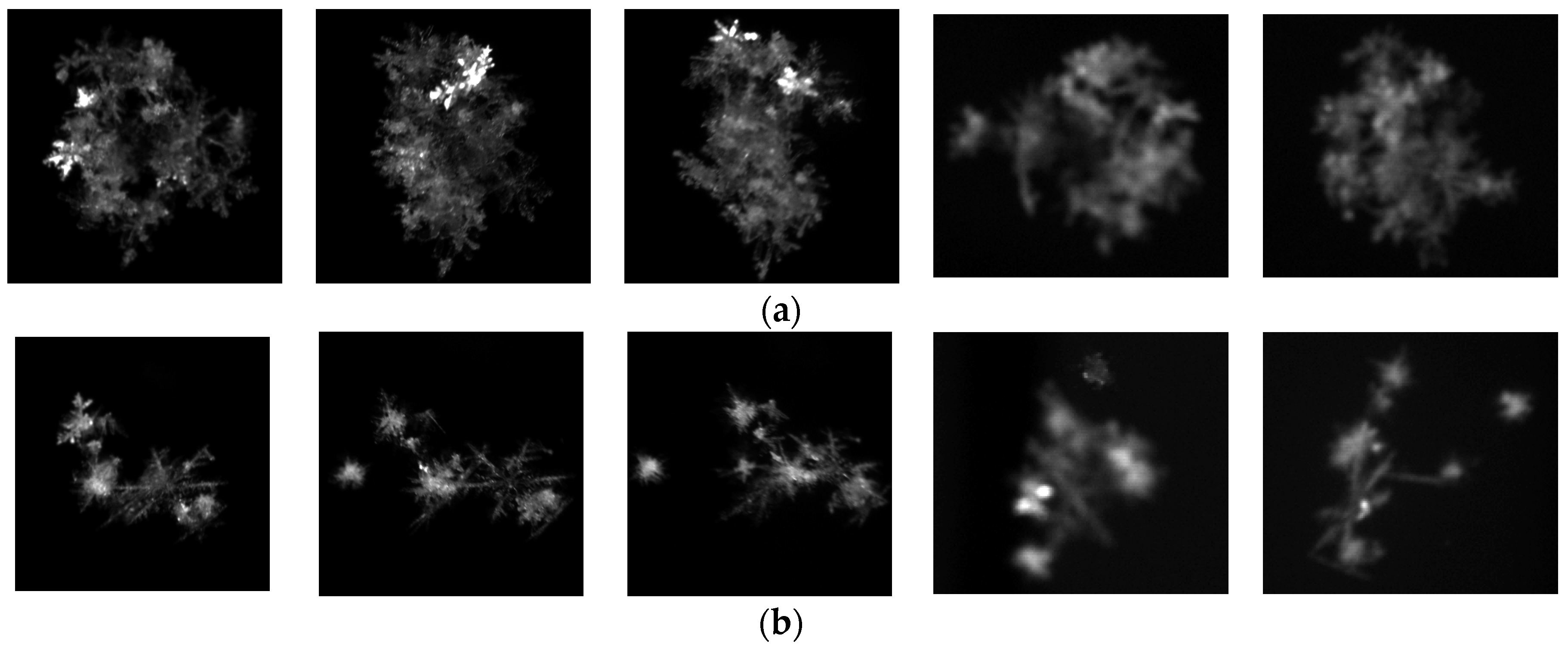
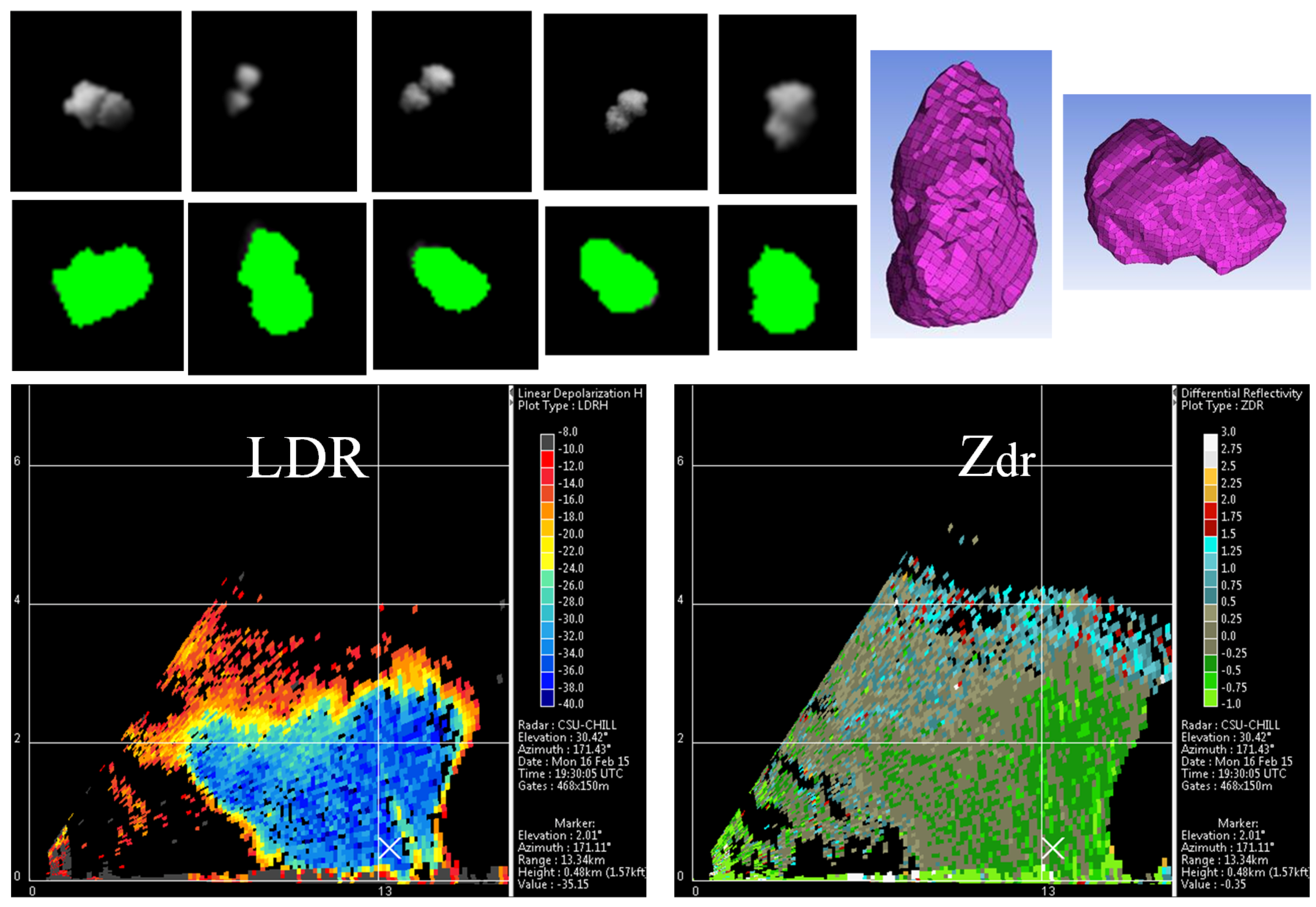
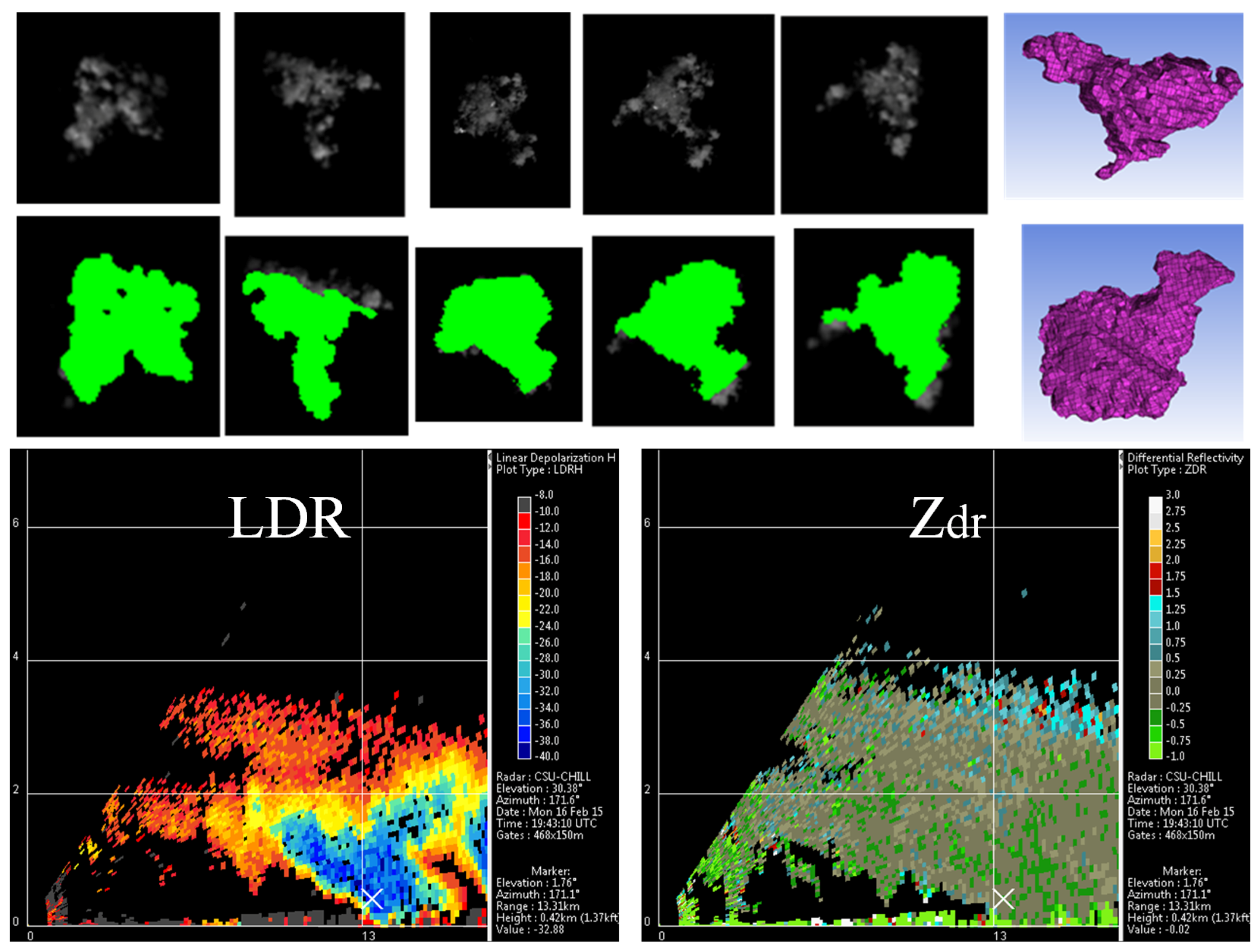
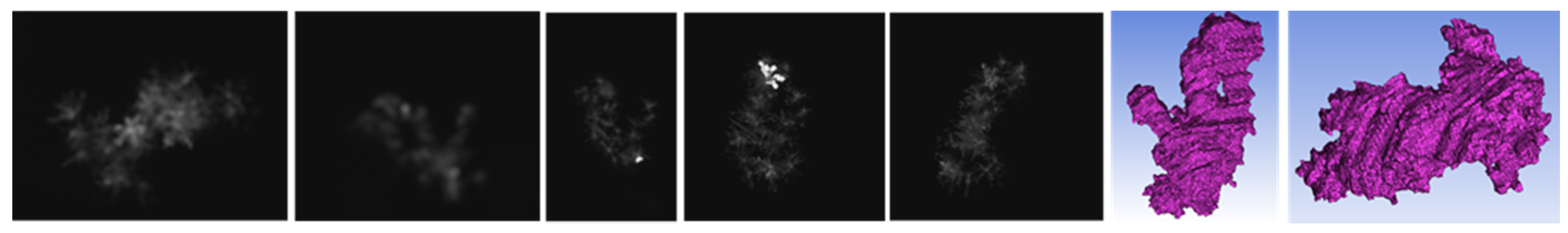
Figure 4 shows two sets of five images of snowflakes collected by five cameras of the new five-camera MASC system during the snow storm on 15 November 2014, at the MASCRAD Field Site. Additional “external” cameras, which took fourth and fifth images in each horizontal panel in the figure, are of much lower resolution (1.2 MP Unibrain Fire-i 785b cameras) than the three original “internal” MASC cameras, and with the same 12.5-mm lenses that were used in the three-camera setup. However, the quality of the additional images is sufficient for the visual hull reconstruction method, where the five image sets substantially improve 3D reconstruction over the three image original MASC output. 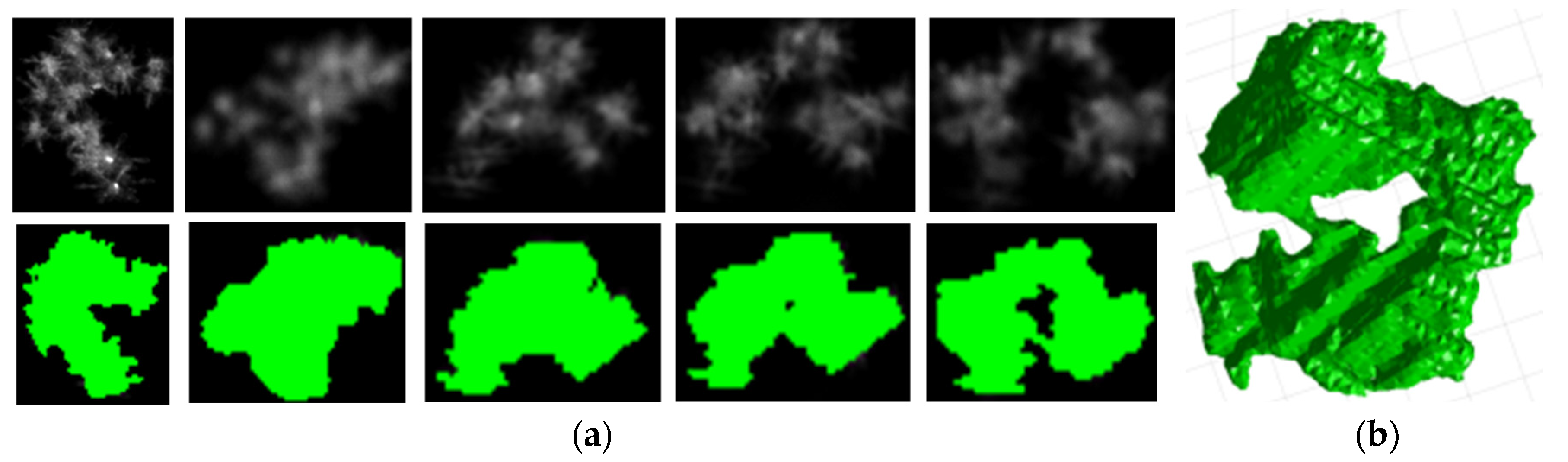Figure 5 shows an example of snowflake shape reconstruction based on five MASC photographs of a snowflake.

Since the surface-based CEM scattering method [27] uses curvilinear quadrilateral meshes, and the final output of the visual hull 3D reconstruction code is a mesh of flat triangular patches, a methodology is developed to convert the VHMC-generated mesh to a mesh with curved generalized quadrilateral patches. First, from the VHMC, a STereoLithography (STL) file is obtained, which gives a triangular mesh representation of the 3D reconstructed snowflake. A TCL script file has been written to take as an input a folder containing multiple STL files and convert them to quadrilateral meshes with no user input using an appropriate meshing technique. For this purpose, commercial ANSYS ICEM CFD software [42] is used. Figure 6 shows examples of 3D shape reconstruction of snow particles using the VHMC code and ANSYS ICEM CFD meshing software. The size of the snowflake is analyzed and meshing parameters are specified based on this size to create a mesh with the desired number of elements in order to adequately represent features of the geometry (Figure 7), as well as to enhance the efficiency of the scattering CEM analysis. We perform mesh error checking, “smoothing” of the mesh, and re-meshing to get a desired, “optimal”, number of elements, from both the geometrical accuracy and the computation efficiency standpoints.

4. Collocated 2DVD for Geometrical and Microphysical Comparisons

The 2D-video disdrometer (2DVD) is described in detail by Schönhuber et al. [13]; Figure 8a shows a 2DVD SN36 model, at the MASCRAD Field Site; a 2DVD schematic is depicted in Figure 8b. Earlier works related to using the 2DVD for snow particles are, for example, [43,44,45]. The instrument computes the particle fall speed and gives two mutually orthogonal images of the particle using high-speed line-scan cameras (Figure 8).

The MASC instrument is relatively new and while it gives high resolution photographs of snow particles, the fall speed and the PSD have yet to be validated by comparison with more established instruments such as the 2DVD. Though the 2DVD has considerably lower resolution (by a factor of 3 for horizontal dimension), it has a much larger sampling area (by a factor of ~3; for MASC, it is approximately 3 cm × 10 cm; for 2DVD, it is 10 cm × 10 cm) and more precise measurement of particle fall velocity. Thus, we installed a well-calibrated 2DVD SN36 (third generation unit) collocated with the MASC, and within the same wind fence, as shown in Figure 9, for cross-comparisons. Figure 10 shows particle collection comparison between the MASC and the 2DVD for selected events during the MASCRAD 2014/2015 snow season, where we observe a satisfactory agreement given the ratio of sampling areas of the 2DVD and the MASC, except in the region with low number of hydrometeors per hour, which might be due to sampling issues playing a more dominant role for low intensity cases (reflected by lower particle counts) and much higher sensitivity of the MASC than the 2DVD for very small particles, e.g., D_eq = 1–1.5 mm. In addition to cross-comparisons, the combination of MASC and 2DVD data enables us to tie microphysical observations with advanced scattering computations through better modelling of snow 3D structure. Moreover, we can use the valuable microphysical statistic properties such as PSD, density-size and fall speed-size relationships obtained by the 2DVD for the MASC data analysis.

We have developed a method for 3D shape reconstruction of ice particles from two orthogonal contour images provided by the 2DVD using a “stacked ellipses” interpolation method [26,47]. Note, however, that this technique, although enabling a better shape model as opposed to the soft spheroid, is much less accurate than that from MASC images (Figure 5) for arbitrary snow particles (it can quite accurately reconstruct the shape of smoother particles, such as graupel). Another caveat is that, for snow particles, it can be used in its current form only under very light horizontal wind conditions due to skewing of the line scan data with even small horizontal particle movement. Still, the volume of the particle is preserved.

5. Winter Precipitation Particle Scattering Analysis Using Method of Moments

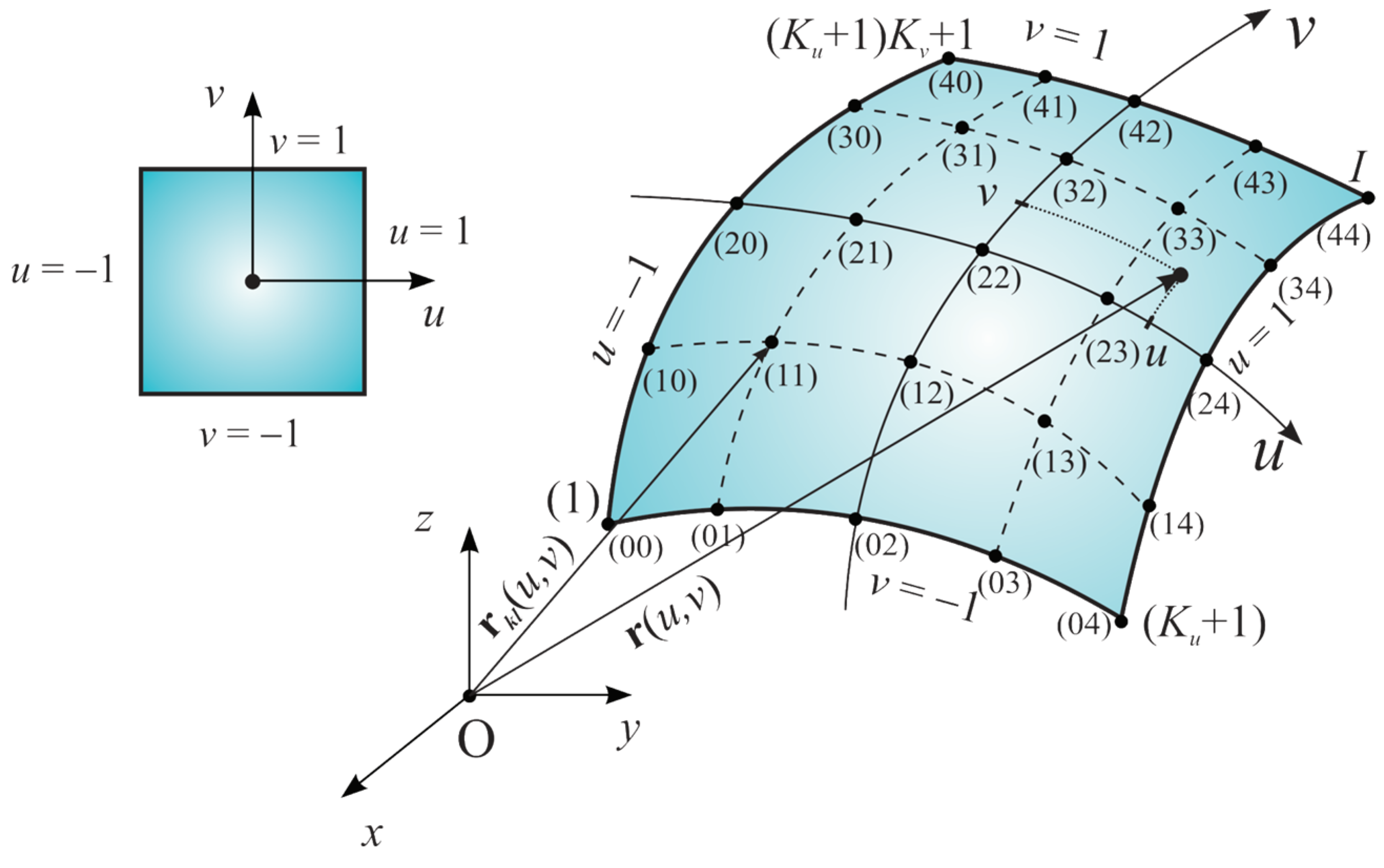
Our scattering models of winter precipitation particles and computation of realistic particle scattering matrices and full polarimetric variables for winter precipitation, focusing only on single particle scattering properties, are based on a numerically rigorous full-wave computational electromagnetics (CEM) approach using primarily the higher order method of moments (MoM) in the surface integral equation (SIE) formulation [27]. In this technique, surfaces of a dielectric scatterer are modeled using generalized curved quadrilaterals of arbitrary geometrical orders K_u and K_v, shown in Figure 11, and electric and magnetic equivalent surface current densities, J_s and M_s, over quadrilaterals are approximated by means of hierarchical vector basis functions of arbitrarily high current-expansion orders N_u and N_v,

$$\begin{gathered} r(u,v)={\displaystyle \sum _{k=0}^{K_u}{\displaystyle \sum _{l=0}^{K_v}{r}_{kl}{L}_k^{K_u}\text{}(u)L_l^{K_v}\text{}(v)}}, \\ {J}_{\mathrm{s}}\text{}=\text{\hspace{0.05em}}{\displaystyle \sum _{i=0}^{N_u}{\displaystyle \sum _{j=0}^{N_v-1}\text{}{\mathsf{\alpha }}_{ij}^{(u)}{P}_{ij}^{(u)}\text{}(u,v)\frac{a_u}{\mathrm{\Im }}}}+\text{}{\displaystyle \sum _{i=0}^{N_u-1}\text{}{\displaystyle \sum _{j=0}^{N_v}{\mathsf{\alpha }}_{ij}^{(v)}{P}_{ij}^{(v)}\text{}(u,v)\frac{a_v}{\mathrm{\Im }}}},-1\le u,v\le 1 \end{gathered}$$

(1)

and analogously for M_s, where L represent Lagrange interpolation polynomials, r_kl are position vectors of interpolation nodes (see Figure 11), P are divergence-conforming polynomial bases, ℑ = |a_u × a_v| is the Jacobian of the covariant transformation, and a_u = ∂r/∂u and a_v = ∂r/∂v are unitary vectors along the parametric coordinates. The unknown current-distribution coefficients {α} in Equation (1) and {β} (for M_s) are determined by solving surface integral equations (SIEs) based on boundary conditions for both electric and magnetic field intensity vectors, employing Galerkin method. Element orders in the model, however, can also be low, so that the low-order modeling approach is actually included in the higher order modeling. For simulations of inhomogeneous scatterers (e.g., melting ice particles), we also use higher order MoM volume integral equation (VIE) modeling [27].

Similarly to the approach described in [15], we use Böhm’s method [17] and the fall speed from the MASC and the 2DVD, as well as the horizontal cross-sectional projected area of the 3D reconstruction of the particle, along with state parameters measured at the MASCRAD Field Site, to estimate the particle mass. In particular, Böhm’s formula for the terminal fall speed depends on three parameters, mass, the mean circumscribed area presented to the flow (A), and the mean effective projected area presented to the flow (A_e), as depicted in Figure 12a. It includes environmental conditions such as air density, viscosity, and temperature. In our analysis process, the bottom view (normal to the flow) is automatically obtained from the reconstructed 3D shape of a snow particle using the visual hull method, as illustrated in Figure 12b. From the mass and volume of the flake, using the volume of 3D reconstructions, we estimate the density, and then the dielectric constant of each snowflake, based on a Maxwell-Garnet formula. Scattering analysis of the 3D reconstructed snowflakes is performed on a particle-by-particle basis by means of the MoM-SIE method and is used to compute polarimetric radar measurables (Z_h, Z_dr, LDR, K_dp, and ρ_hv). These results are compared against the corresponding data collected by the CSU-CHILL radar.

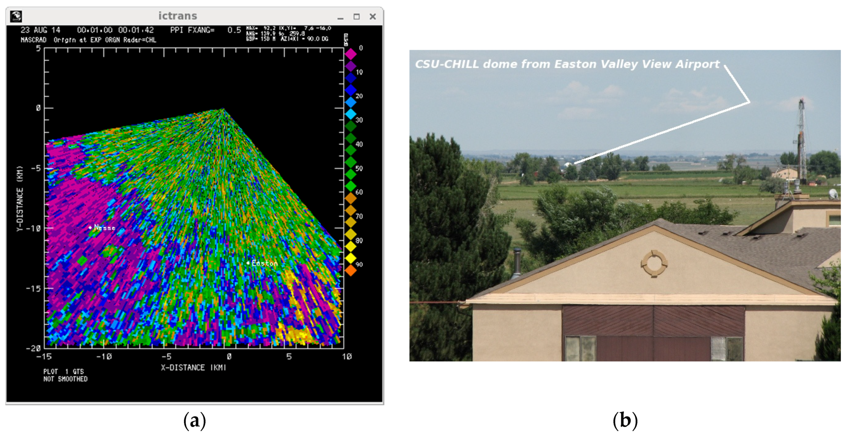
6. Establishing MASCRAD Easton Surface Instrumentation Snow Field Site

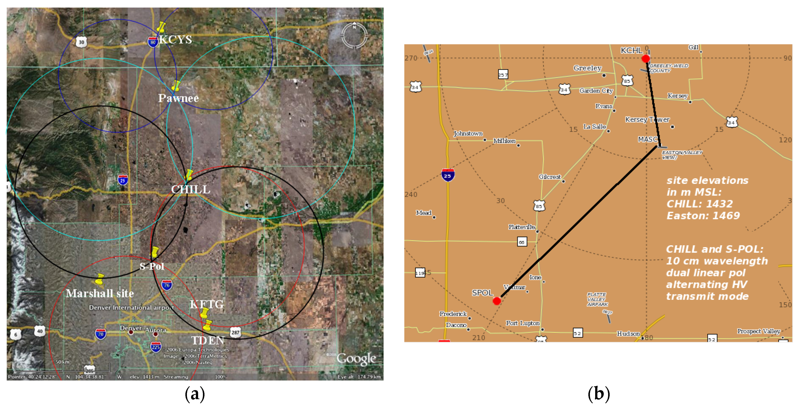
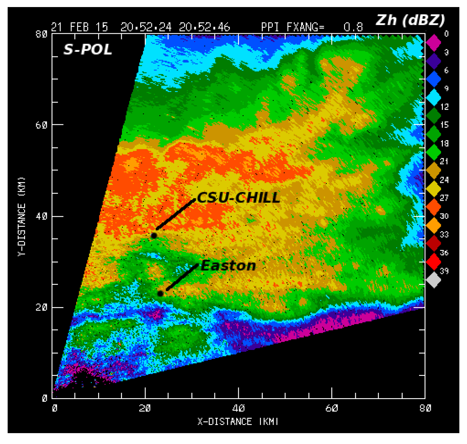
Out of several possible locations, the requirement that the MASCRAD surface instrumentation site be located within the view of CHILL and SPOL radars led to two best candidate sites, the “Nesse site” and the “Easton site”, at a range of 14.88 km and 12.92 km, respectively, from the CHILL Radar (Figure 13a). 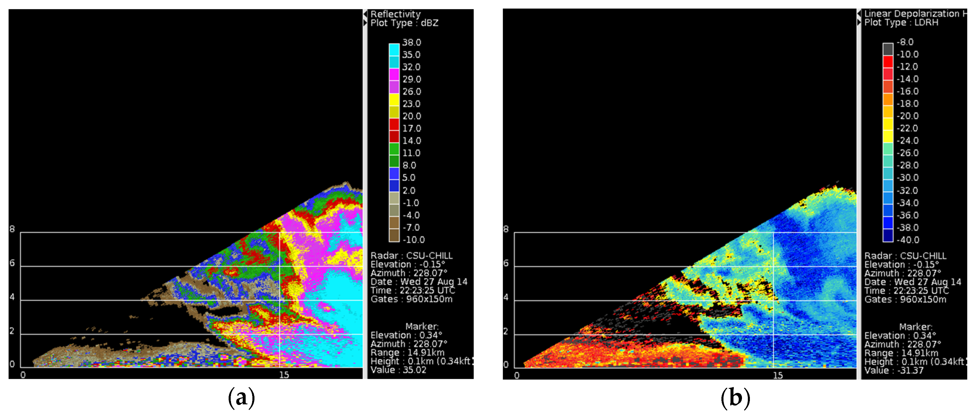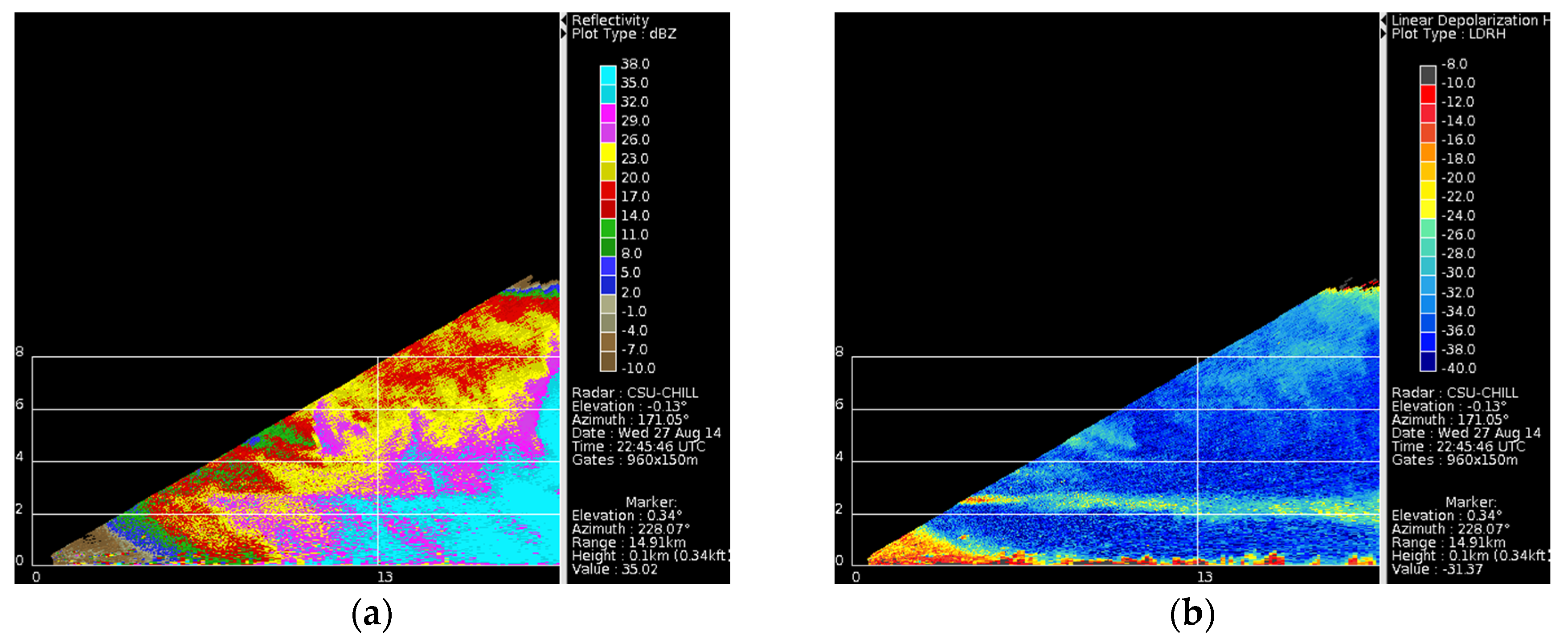Overall, the ground clutter was by far the predominant reason which resulted in the selection of the Easton Valley View Airport, a small airport for crop dusting airplanes in La Salle, Colorado, shown in Figure 13b, for the MASCRAD project. To evaluate ground clutter effects, rain of varying intensity was observed by the CHILL Radar at the two candidate MASCRAD sites over several days in late August 2014, as shown in Figure 14 and Figure 15. It appeared that due to clutter and beam blockage effects, becoming more apparent as the meteorological echo strength weakened, LDR measurements could be made to lower signal levels at the Easton site when compared to the Nesse site. In order to clear the ground clutter, CHILL radar had to point at a higher elevation angle at the Nesse site than at the Easton site. The Easton site is located on a ridge, and, from the right location, one can see the radome of the CHILL antenna. At the Easton site, the elevation angle of the radar can be kept noticeably lower, which allows for the beam to be closer in height to the measurement area of the MASC and 2DVD, minimizing difference between the snow in the radar pulse volume versus the snow measured by the MASC/2DVD.

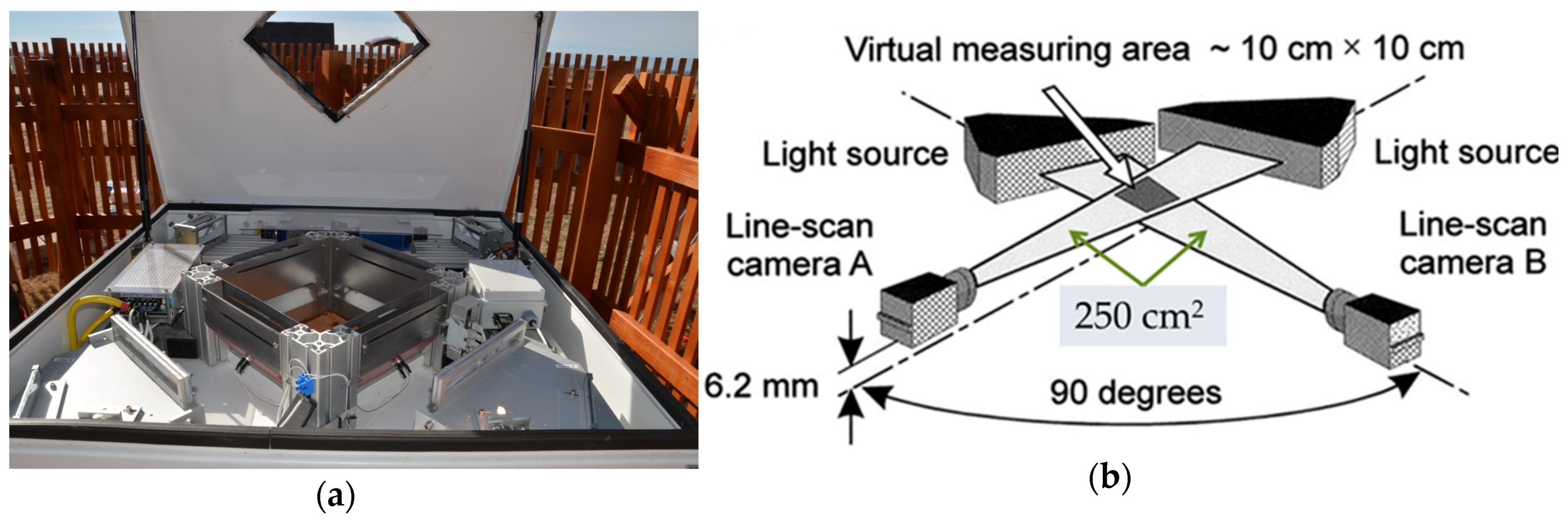
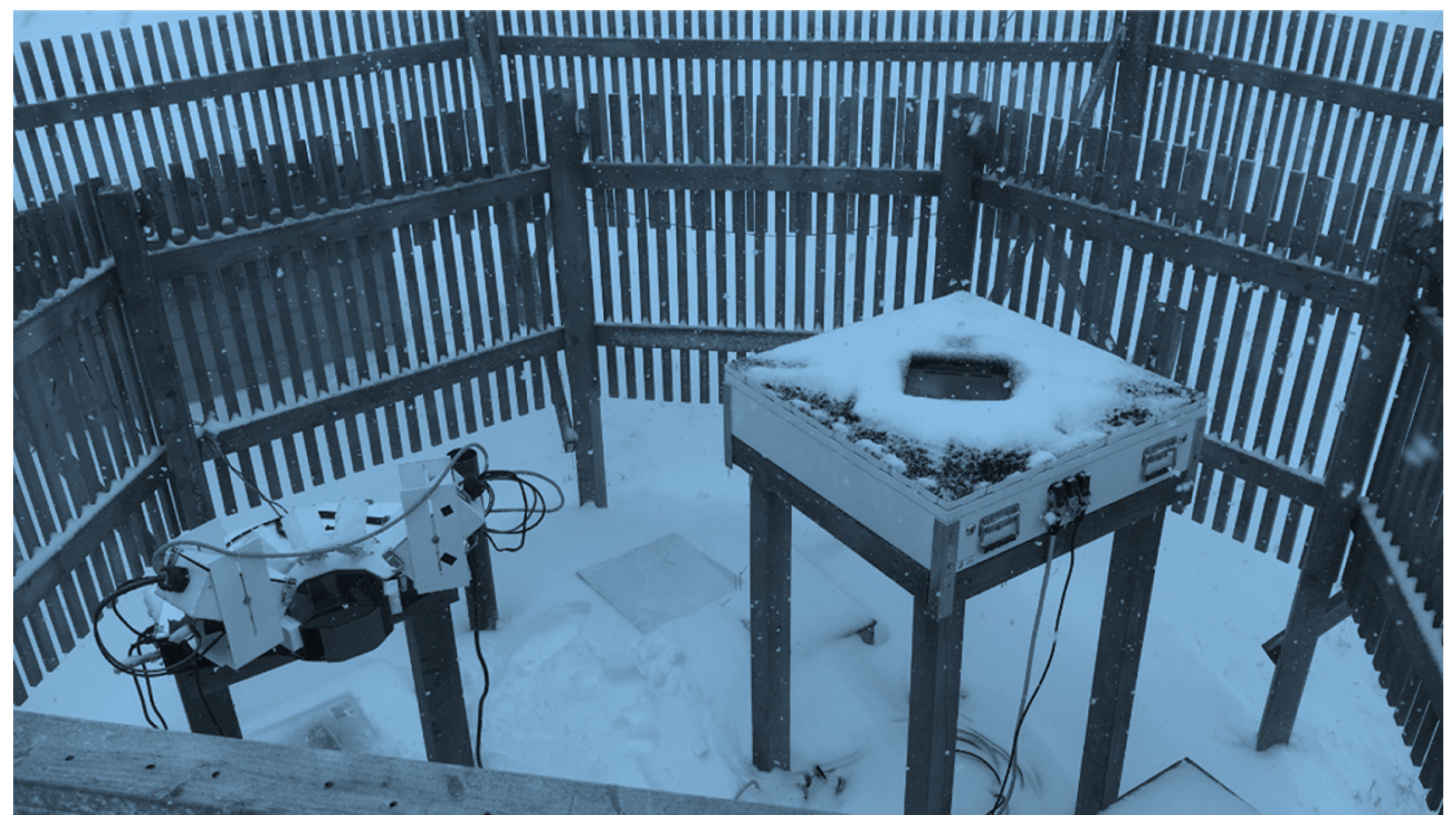
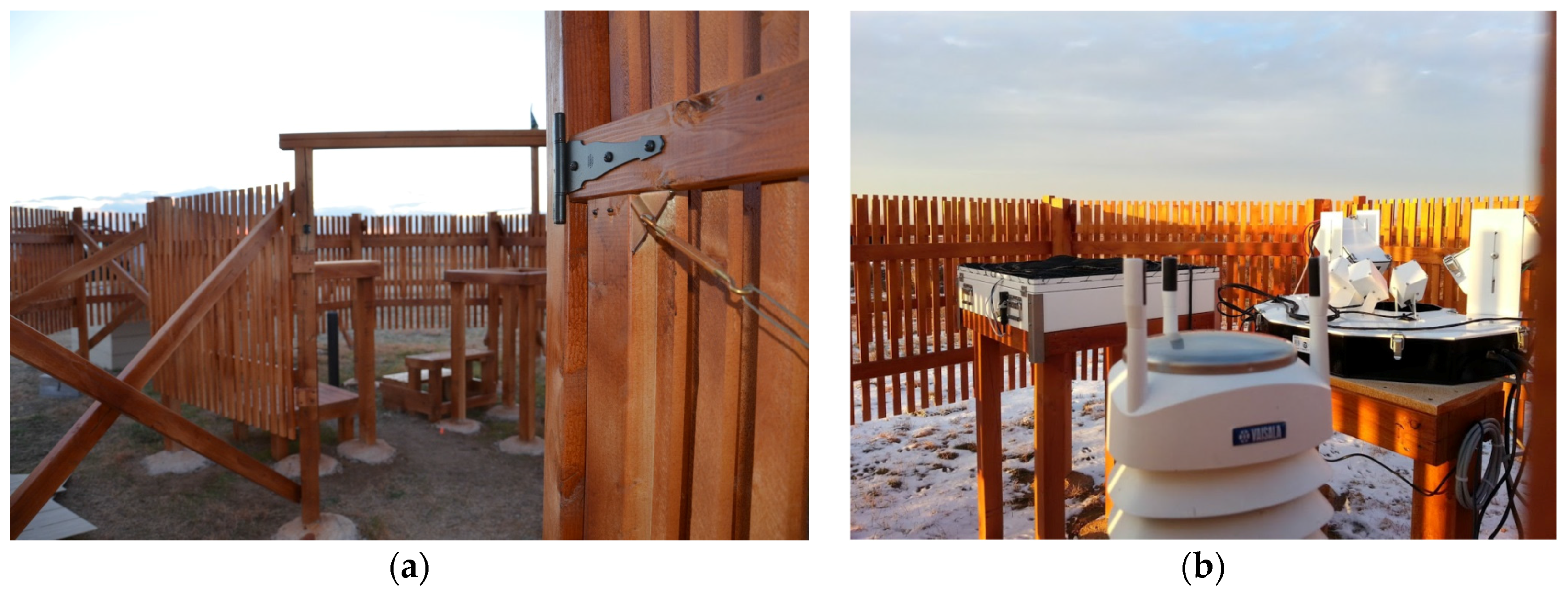
We constructed the MASCRAD Field Site at the Easton Valley View Airport, south of Greeley, Colorado, shown in Figure 16, in October 2014 [23]. We built a 2/3-scaled (8-m outer diameter) double fence intercomparison reference (DFIR) wind shield [48] at the site, for placement of the MASC (Figure 1), 2DVD (Figure 8), PLUVIO200 snow measuring gauge (a weighing-type gauge, which provided conventional precipitation accumulation measurements vs. time for the campaign), and VAISALA weather station, as well as a big heated weather-proof enclosure for the two computers running the MASC and the 2DVD and other accessories. The purpose of the DFIR shield is to reduce the impacts of horizontal wind on the collection efficiency of the hydrometeor sensors. We also used the collocated NCAR GAUS (GPS advanced upper-air system) sounding system. The GAUS facility provided important high-resolution measurements of temperature, humidity, pressure, and winds. It is well-known, for example, that the vertical profile of wet-bulb temperature will constrain the type of precipitation at the surface. 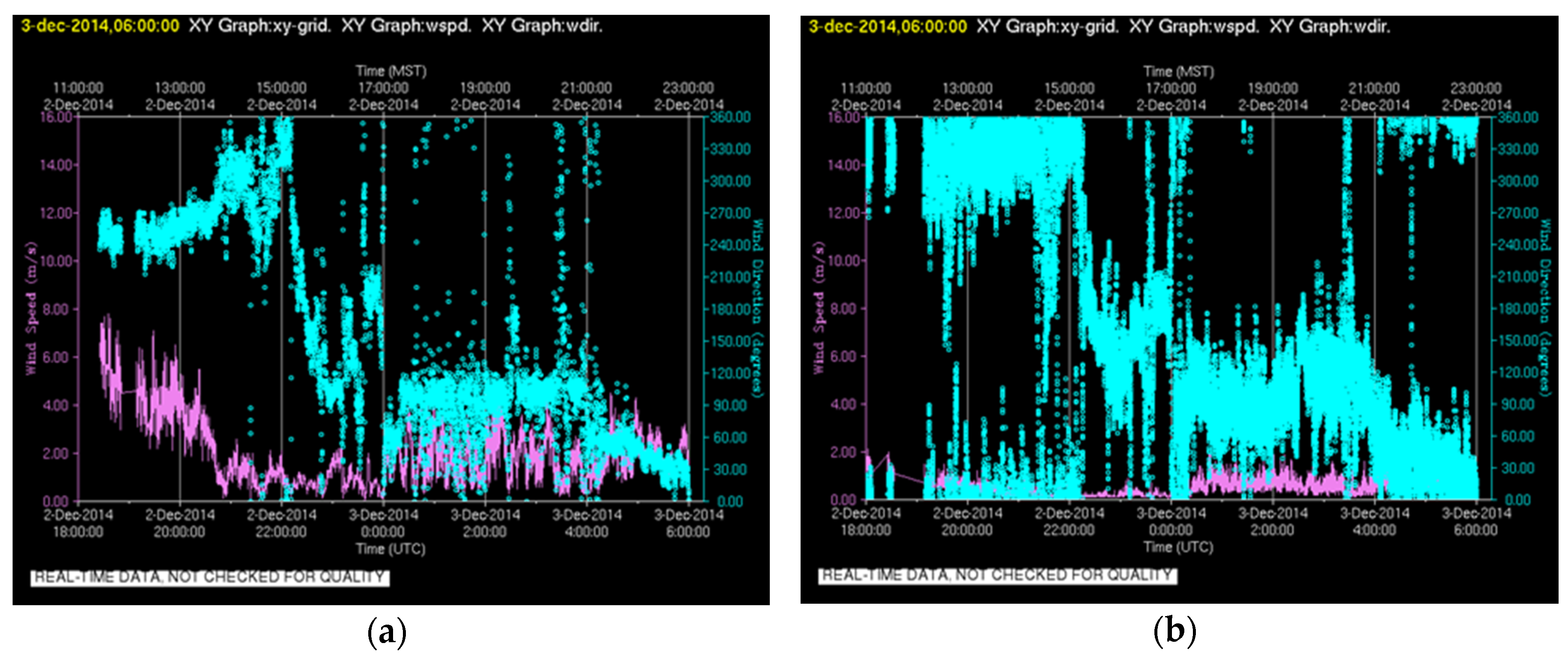Figure 17 shows characteristic plots of the GAUS measured wind speed data at the MASCRAD Snow Field Site, outside and inside the DFIR wind fence, from which a threefold (or more) wind reduction inside the fence relative to the outside environment is observed; this is typically observed in all high-wind events during the 2014/2015 winter season. The MASCRAD Field Site was fully operational and performed well during the first snow storm of the season, on 15 November 2014.

7. Scans over MASCRAD Field Site by Two State-of-the-Art Polarimetric Radars

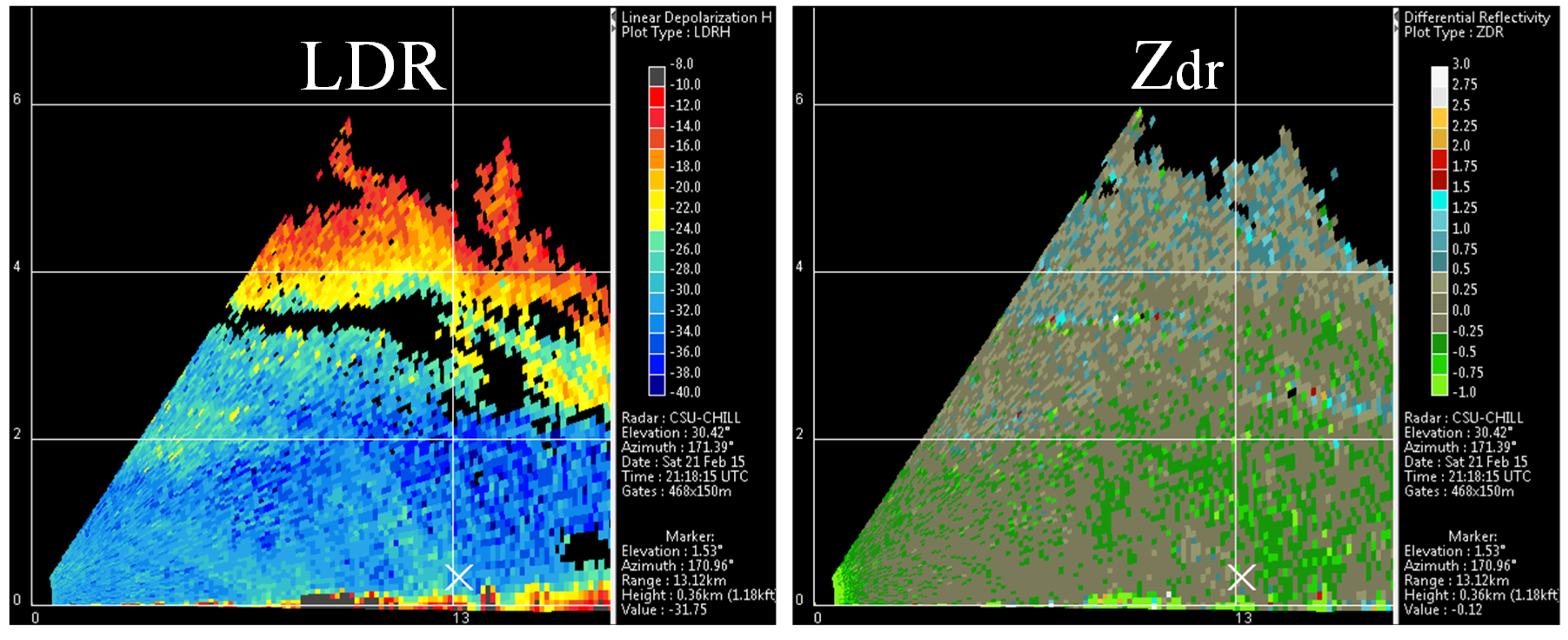
The newly built and established MASCRAD Easton Field Site is conveniently located in-between the CSU-CHILL and NCAR SPOL radars, as shown in Figure 18. The CSU-CHILL radar is the primary radar for the project, while the SPOL radar provides for additional polarimetric radar coverage as well as the capability of dual-Doppler derived wind fields. The CSU-CHILL radar with the high performance S-band feed was used to scan (with high resolution) precipitation over the instrumented site. The very high quality LDR measurements are needed to see if subtle changes in particle riming can be corroborated with MASC data, and if freezing rain or a re-freezing layer can be detected by CSU-CHILL and corroborated with the MASC images—as two characteristic examples. The SPOL radar provides broader coverage and at times the two radars are scanned to obtain dual-Doppler wind fields.

The CSU-CHILL radar is a two-transmitter, two-receiver system that measures the full covariance matrix in either H/V or slant linear 45°/135° basis. The antenna is an 8.5 m dual-offset Gregorian design with very high polarization purity and excellent side-lobe performance in any plane [50]. The measured LDR system limit is estimated to be −40 to −43 dB, while the two-transmitter firing alternately every PRT prevents any cross-coupling errors in Z_dr, present in simultaneous transmit systems such as the WSR-88D [51,52], and avoids depolarization streaks in Z_dr/ρ_hv due to crystals aligned off the horizontal or vertical directions [53]. In addition to the two examples mentioned above, note that it has long been recognized that the measure of the LDR is highly sensitive to particle riming or melting, to irregular shapes such as dry snow aggregates, to ice crystal morphology, to aspherical ice pellets or lump graupel, and, in the extreme case, to freezing rain [4,54,55].

For collection of CHILL and SPOL radar data for the MASCRAD project, for the 2014/2015 MASCRAD winter campaign, special scan strategies were implemented for both radars focused on high spatial and temporal resolutions over the Easton site. For CHILL, the dual-transmitter PRFs were increased to 1000 Hz each. In alternating pulse mode, the effective PRF is 2000 Hz to enable coherent processing gain to extract weak cross-polar signal from noise (improving LDR detection). All data over the Easton site was being acquired in time series mode (I + jQ) in addition to conventional covariance products. The scan strategy over Easton included three fixed pointing beams with dwell of 20 s each, 2 RHIs, 1 low elevation angle PPI sweep, and 1 VAD scan. This cycle repeated every 4 min. The SPOL radar (PRF = 1000 Hz; alternating mode using fast polarization switch) scans included PPI sectors at 7 elevation angles (60° sector centered at Easton) along with 2 RHIs. Time series data were archived routinely. Additionally, the WSR-88D radars in Denver, Colorado, and in Cheyenne, Wyoming (see Figure 18), provided secondary validation data over the Easton measurement site.

The MASCRAD Easton Field Site is at azimuth 171.3°/range 12.92 km from CSU-CHILL. The ground elevation at the Easton Airport is ~32 m higher than the terrain height at CSU-CHILL. Due to ground clutter, the lowest elevation angle at which uncontaminated meteorological data can be collected with the CSU-CHILL S-band system in the immediate Easton vicinity is 1.5° (of course, our goal is to reduce as much as possible the vertical separation between the radar sample volume and the surface-based measurements). At this elevation angle, the antenna pattern’s main lobe is located between the ~192 m and 420 m heights above the ground at the Easton site. When precipitation was occurring or expected at Easton, both CSU-CHILL and SPOL radars conducted pre-programmed, ~4 min cycle time scan sequences that included both low-elevation angle PPIs as well as narrow RHI volumes centered on the ground instrumentation site.

8. Illustrative Results from 2014/2015 MASCRAD Winter Campaign and Discussion

Using either individual or coordinated operations, the CSU-CHILL and NCAR SPOL radars collected dual polarization data—coupled with in-situ surface measurements performed at the MASCRAD Field Site—during essentially all significant snow events that occurred in the greater Easton Airport area between November 2014 and April 2015. The following three cases were selected to illustrate MASCRAD observations and computations during the 2014/2015 MASCRAD winter campaign, as well as the diversity of hydrometeor types that were processed and analyzed.

8.1. Example Case 1 of MASCRAD Observations and Computations: Unusual Winter Graupel Shower Event on 16 February 2015

During the pre-dawn hours of 16 February 2015, a well-defined 50 kPa upper trough system moved southward across the MASCRAD Field Site [28,29]. The operational NWS sounding data at 12:00 UTC on the 16th, indicated that mid-tropospheric cold air advection was occurring over northeastern Colorado. The resultant thermal instability was forecast to increase later in the day as solar heating of the ground surface occurred. (Surface temperatures were expected to remain just below freezing). This forecast instability was realized in the active development of cumulus clouds, some with visible precipitation shafts, in the vicinity of the CSU-CHILL radar site around 18:00 UTC. By 18:31 UTC, small convective echoes with maximum core reflectivities of ~35 dBZ existed along a line located just south of the MASCRAD Easton site (Figure 19). Similar small shower echoes affected many locations in the general Greeley–Denver region on the afternoon of 16 February. Based on the reports filed by observers in the Community Collaborative Rain, Hail and Snow (CoCoRaHS) network, a number of these showers generated graupel.

Additional showers began to develop near the MASCRAD Easton site at ~18:40 UTC. In response to these local developments, CSU-CHILL scanning that repeated RHIs over the Easton site with a cycle time of ~2.25 min were started. The vertical structure of one of the convective echoes that affected the Easton site at 19:27 UTC is shown in Figure 20. Echo height was relatively low, extending to only slightly above 4 km height above ground level (AGL). An elevated region of more intense reflectivity, reaching levels of ~30 dBZ, was found in the leading portion of the echo system near the 2 km AGL level. This elevated reflectivity maxima appeared to be the source region for curving columns of enhanced reflectivity that reached down to the surface. Differential reflectivity values tended to be fractionally negative in this same higher-intensity, overhanging reflectivity at the leading edge of the system (i.e., between ranges 12 and 15 km in Figure 20). Generally similar reflectivity and Z_dr structures were seen in two other showers that passed through the RHI scan planes between 19:00 and 20:15 UTC. The accuracy of the CSU-CHILL system Z_dr calibration was checked using vertically-pointed data collected during a snow event six days later. Based on this vertically-pointed data, +0.2 dB was added to the values in the archive data files. This adjustment has been applied to the plots shown in Figure 20. The fractionally negative Z_dr values in the echo cores are also consistent with those observed by the NWS KFTG radar in this event. This pattern of low-topped convection containing slightly negative Z_dr values and producing reports of conical graupel at the surface has been reported by Evaristo [56].

The descending reflectivity cores observed on 16 February 2015 were never well-centered on the Easton site; as a result, the MASC only collected ~50 particle images during the ~19:00–20:15 UTC period. Within this small sample, lump type graupel particles were frequently observed (Figure 21). Analysis results indicate the axis ratio of the graupel particles tended to become slightly prolate with increasing diameter. This shape characteristic accounts for the fractionally negative Z_dr values that were observed [29].

Figure 22 and Figure 23 show illustrative results of MoM-SIE scattering calculations based on the MASC images captured at the MASCRAD Field Site during the unusual winter graupel shower event on 16 February 2015, in comparison with CSU-CHILL radar data [30]. As can be seen, the computed LDR and Z_dr single-particle values (given just for illustration; the full analysis based on all collected particles for the event is ongoing) agree well with those measured simultaneously by the radar.

8.2. Example Case 2 of MASCRAD Observations and Computations: Major Snow Band Passage Event on 21 February 2015

The second MASCRAD project example case took place on 21–22 February 2015, when a major snow band associated with a cold frontal passage moved across the MASCRAD Field Site [28]. Figure 24 shows the low-level reflectivity pattern observed by the NCAR SPOL radar as the leading edge of this snow band was just reaching the CSU-CHILL site at 2015 UTC. The reflectivity values in excess of 30 dBZ were some of the highest levels observed from snow echoes during the 2014/2015 MASCRAD winter campaign.

Shown in Figure 25 is an RHI scan taken by the CSU-CHILL radar as the maximum reflectivity portion of the snow band was in the vicinity of the MASCRAD Easton site (range 12.92 km). Areas of light snow were fairly widespread before the surface cold front and primary snow band arrived in the Greeley area near 21 UTC. The arrival of the cold front brought northerly winds gusting to ~15 m/s and markedly reduced visibility in moderate to heavy snow at the CSU-CHILL site. The RHI data showed an echo depth increase of 1.5–2 km in association with the arrival of the snow band. Differential reflectivity was consistently near 0 dB in the lowest ~1 km in the higher reflectivity portions of the snow band.

Selected MASC images from this high-reflectivity period are shown in Figure 26. These images contain relatively large diameter particles with good focus and illumination. The larger diameter particles were of interest since they primarily influence the radar return signal. The MASC images during the passage of the high reflectivity axis of the snow band were typically rimed aggregates. Based on the MASC’s rapid flash rate, particle concentrations were high. The irregular shapes and orientations of these aggregates are consistent with the observed near 0 dB Z_dr values.

A comparison of the Z_dr values observed in the 16 February 2015 graupel showers and in the 21 February 2015 snow band is shown in Figure 27. Both events have a mode Z_dr value that is very close to 0 dB. The 16 February case, which contained more lump graupel particles than aggregates, had a longer tail of values extending into the negative Z_dr range.

Similar histograms for the LDR are shown in Figure 28. The snow band case (blue trace) shows slightly higher depolarization levels. This is related to the more irregular/less spherical shapes of the large aggregates that were documented in the snow band.

In addition, we performed the microphysical characteristics analysis of the 21–22 February 2015 heavy snowfall case, with the objective to quantify the vertical structure of precipitation and the snow characteristics at ground level and link one to the other. The precipitation vertical structure was obtained from the CSU-CHILL radar RHI scans and the ground snow characteristics from the 2DVD (to characterize PSD at the ground) and the MASC (to classify habits of snow particles at the ground). Quality control of the 2DVD data was performed in a step-by-step procedure, details of which are given in [57].

Past studies have shown that the dominant microphysics processes at heights above the −15 °C level are different from those below it [9]. In the region warmer than −15 °C height, ice particles mainly grow from aggregating or riming. At colder temperatures, ice particles predominantly grow from diffusion process. To measure microphysics of two regions, temperature profile data observed from sondes launched at the MASCRAD Field Site is used. From temperature profiles, −5 °C, −10 °C, and −15 °C heights are found and the radar reflectivity gradients are calculated for the corresponding heights.

The ground snow characteristics were quantified by (a) PSD; (b) particle velocity distribution; (c) intercept parameter N_w (= (4⁴/Γ(4))(M₃)⁵(M₄)⁻⁴, m⁻³·mm⁻¹) of the PSD; (d) apparent mass-weighted mean diameter D_m (= M₄/M₃, mm), which is proportional to the degree of aggregation; and (e) mean fall velocity, which is proportional to the degree or riming [58], where M_n is n-th moment of the PSD.

From the regular RHI radar scans, such as the one shown in Figure 29a, the height-time indicator extracted over the MASCRAD Field Site was obtained. This indicator can clearly show precipitation vertical structure change above a specific location. Precipitation vertical structure changes influence the ground snowfall properties, thus the height-time indicator can be used to find quantitative relationships between the precipitation vertical structure and the ground snow characteristics. In our analysis, we have taken into account the finite time for the snow particles to fall from a given height to reach the ground level. Figure 29b,c show the height-time indicator for the horizontal reflectivity, Z_h, and the differential reflectivity, Z_dr, for the event, where several points can be made observing the results. First, this indeed is a very heavy snowfall case because Z_h is greater than 30 dBZ close to the surface. Second, there appear to be some high positive Z_dr regions and some negative Z_dr regions. High Z_dr implies that ice particles have significant oblateness and is seen at cloud top heights. A negative Z_dr area indicates ice particles like conical graupel or heavily rimed aggregates with the major axis in the vertical and the area is often seen in mid-cloud regions (see, for example, Figure 26).

Figure 30 shows the relation between precipitation vertical structure and ground snow characteristics, namely, the scatterplots of the linked gradient of the horizontal reflectivity, ∇Z_h (dB/km), computed using the radar variable values of −10 °C and −15 °C isotherm heights h as ∇Z_h = (Z_h(−10 °C) − Z_h(−15 °C))/(h(−15 °C) − h(−10 °C)), versus D_m and versus N_w, respectively, for the 21–22 February 2015 event. We observe from the figure that ∇Z_h increases with D_m, but decreases with N_w, which means that the radar signatures show high ∇Z_h when aggregation becomes the dominant microphysics.

Figure 31 shows the time series of the PSD and particle velocity distribution for the 21–22 February 2015 event. Figure 31b also includes some MASC images. MASC images at around 15 h UTC show aggregated snowflakes. At the same time, the mean fall velocity had low values, although the PSD had narrow distribution. MASC images of 22 h UTC show aggregated snowflakes with riming. Within that timing, the PSD had wide distribution and it was observed to have high fall velocity.

Figure 32 and Figure 33 show characteristic examples of MoM-SIE single-particle scattering calculations based on the MASC images captured during the 21 February 2015 major snow band passage event, in comparison with results measured simultaneously by CSU-CHILL radar [30]. Again, while a good agreement can be observed, these examples are given just for illustration, as the scattering analysis of all collected particles for the event is ongoing.

8.3. Example Case 3 of MASCRAD Observations and Computation: Positive Z_dr in Dissipating Light Snow Area on 3 March 2015

In contrast to the two previous “active” cases in which local convection (16 February 2015 graupel showers) and well-organized frontal lifting (21 February 2015 snow band) were occurring, the final event took place as an area of light snow was fading in terms of horizontal extent and reflectivity [28]. On the morning of 3 March 2015, an area of light to moderate snow had passed the MASCRAD Field Site while moving from north to south. By ~18:00 UTC, only a shallow (~1 km deep), low reflectivity (single digit positive Z_h values) remained over the Easton site. Within this tenuous residual echo layer, Z_dr values were distinctly positive, with isolated maximum values of ~+5 dB (Figure 34). Quantifications of Z_h and Z_dr values observed in this layer near Easton are shown in Figure 35.

Figure 35 highlights that aggregation is occurring. Namely, an increase in Z_h and respective decrease in Z_dr cannot happen with diffusional growth of dendrites/plates [59]. In other words, when reflectivity is low, the particle number concentrations are small, reducing the frequency of particle collisions/aggregation. When these “aggregational” collisions do not occur, the intrinsic positive Z_dr characteristics of the individual crystals are more evident.

This shallow, low reflectivity environment reduced the probabilities of particle riming and collisions. The selected MASC images shown in Figure 36 have more readily apparent individual crystal components vs. the heavily rimed aggregates seen in the snow band of 21 February 2015. The more pristine, planar crystal forms on 3 March 2015 would be expected to fall in a maximum-drag/quasi-horizontal orientation [60]. This fall mode would produce the distinctly positive Z_dr values that were observed in the CSU-CHILL data. While the surface temperature was near −6 °C, NWS Denver sounding data at 00:00 UTC indicated that temperatures at the ~1.4 km AGL (2.8 km MSL) echo top level were ~−13 °C. The pristine, single crystals likely grew primarily in the −10 to −15 °C temperature range in near the top of the echo layer, then maintained their flat/positive-Z_dr aspect ratios as they descended to the ground (with infrequent collisions).

Figure 37 and Figure 38 show illustrative results of MASC/MoM-SIE single-particle measurements/calculations for the 3 March 2015 event, in comparison with CSU-CHILL radar data [30].

9. Conclusions

This article has proposed and presented a novel approach to the characterization of winter precipitation and modeling of radar observables through a synergistic use of (1) advanced optical disdrometers for microphysical and geometrical measurements of ice and snow particles; (2) visual hull image processing methodology; (3) advanced MoM-SIE computational electromagnetics scattering computations; and (4) state-of-the-art polarimetric radars. The article has also described the newly built and established MASCRAD surface instrumentation snow field site, which includes a MASC, 2DVD, PLUVIO snow gauge, and VAISALA weather station, within a DFIR wind fence, and the collocated NCAR GAUS sounding system, under the umbrella of CSU-CHILL and NCAR SPOL polarimetric weather radars. This site has then been augmented by advanced geometrical and image processing and scattering modeling and computing capabilities.

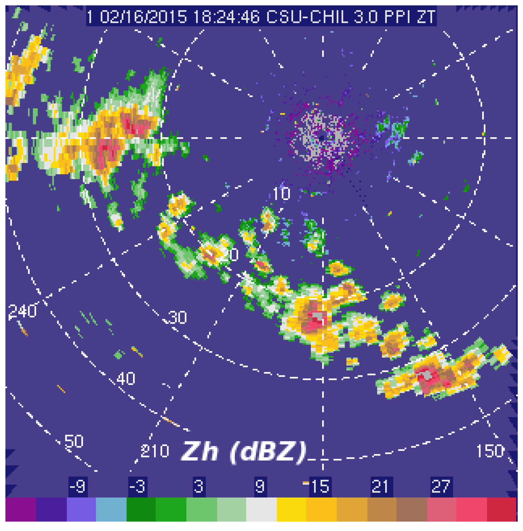
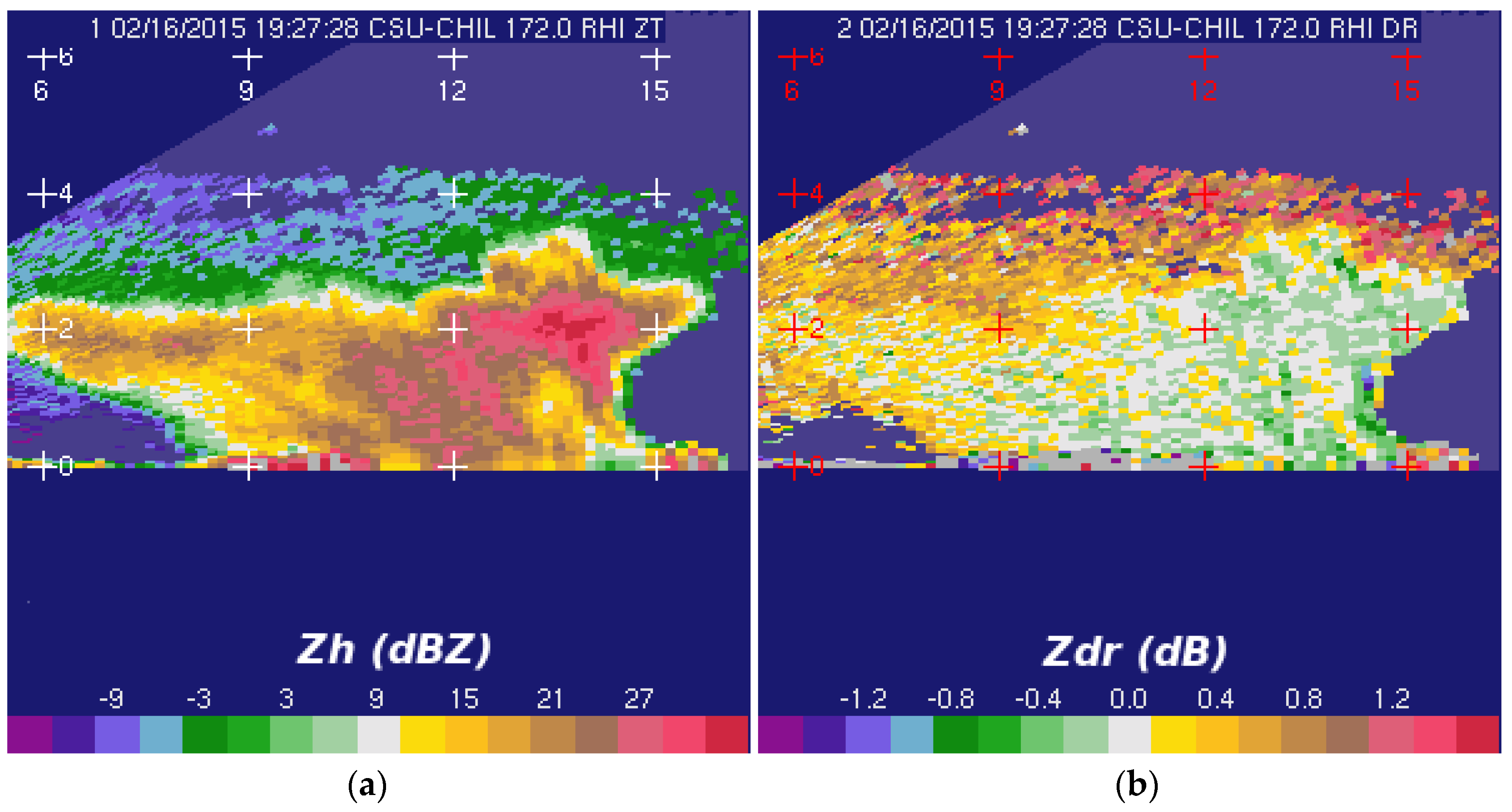
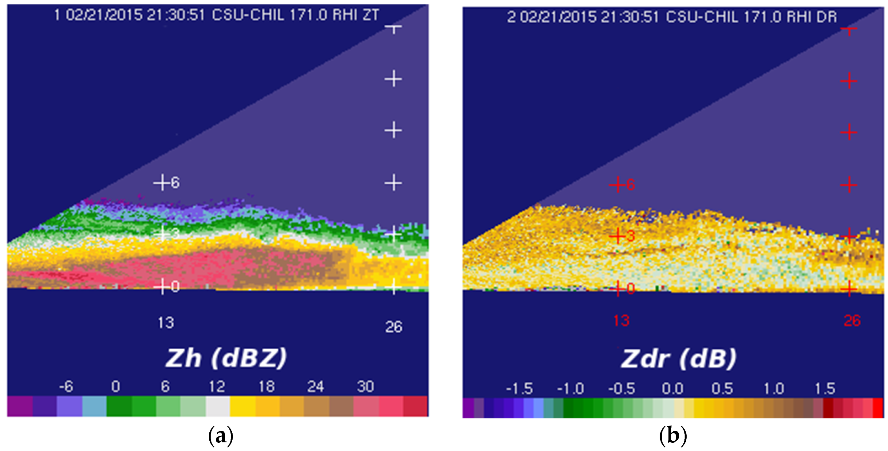
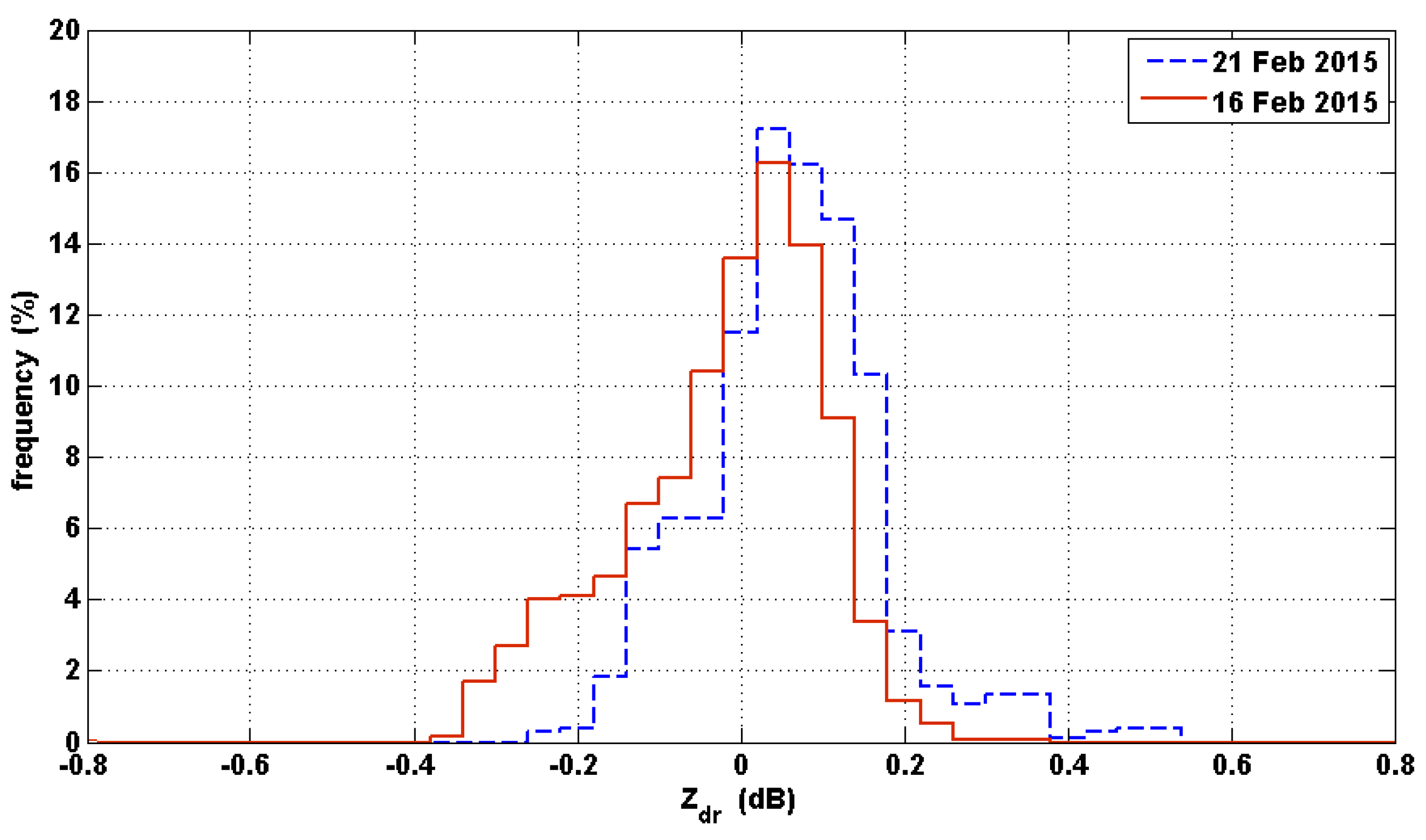
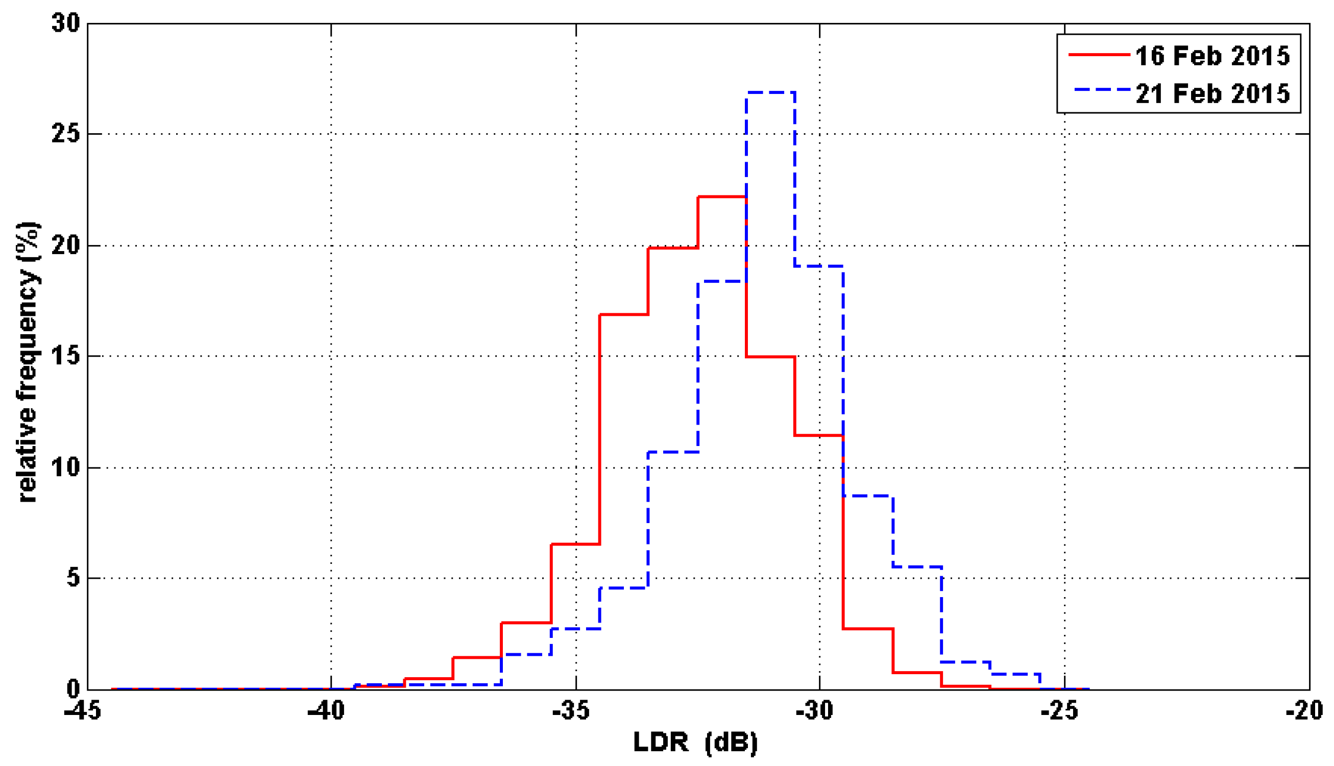
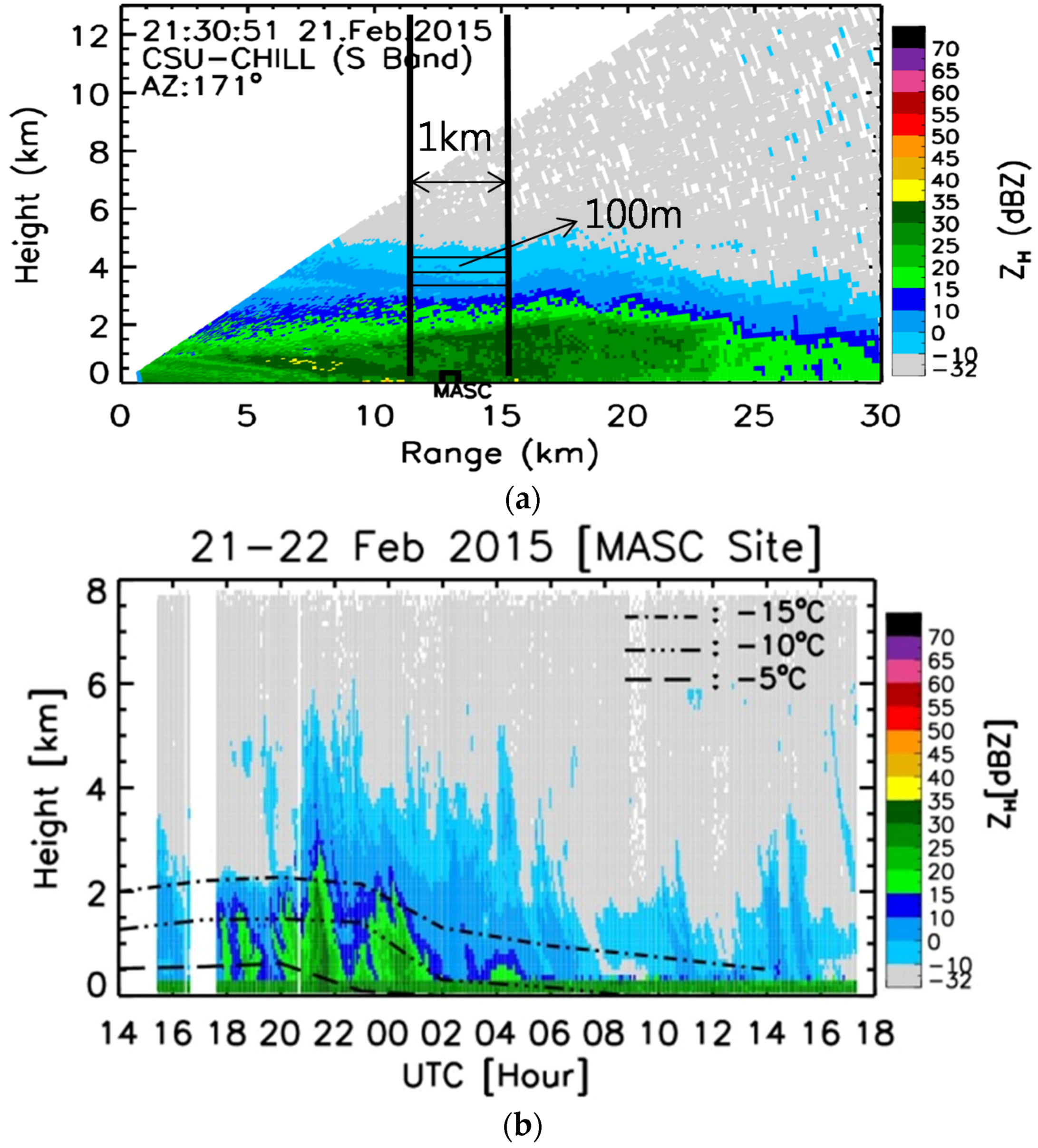
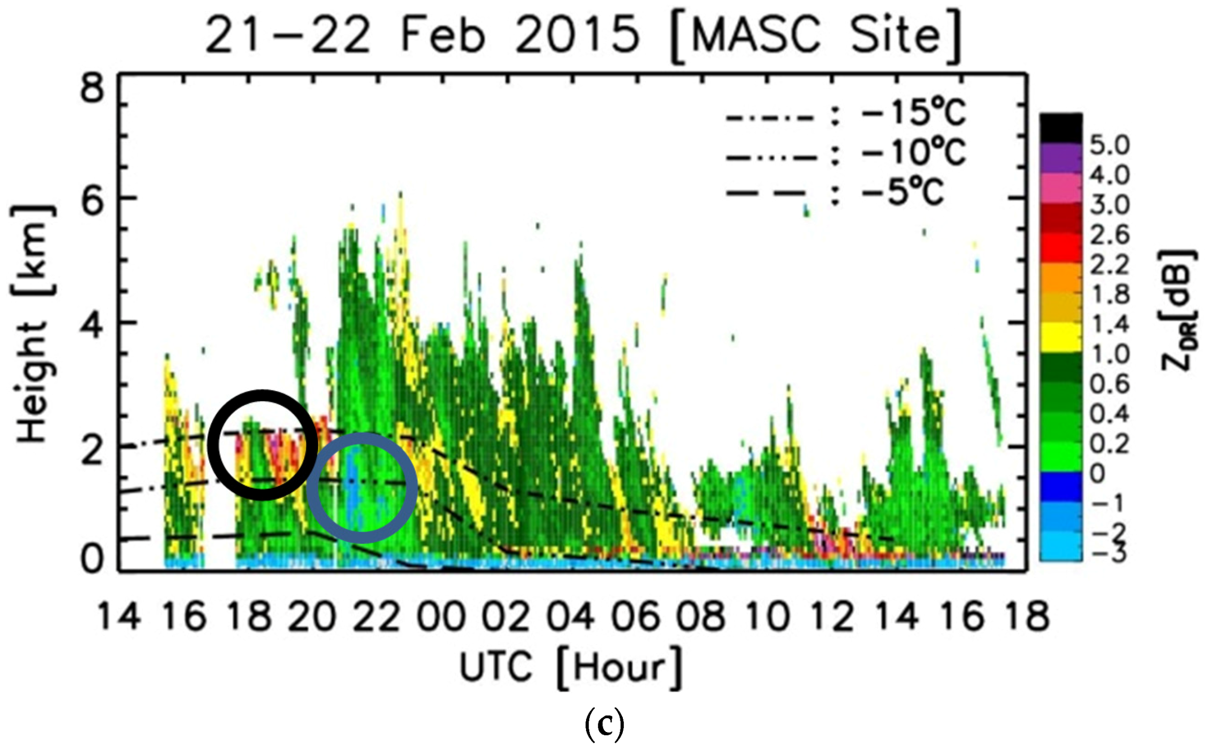
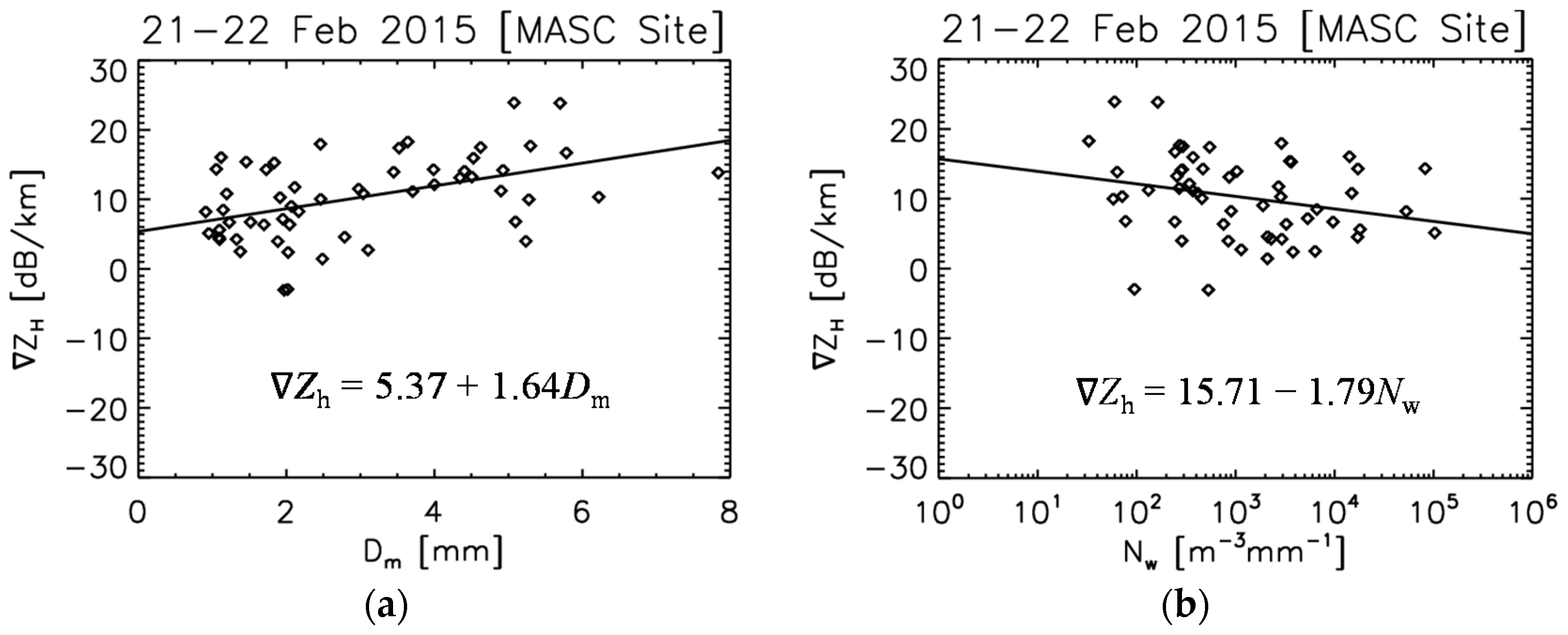
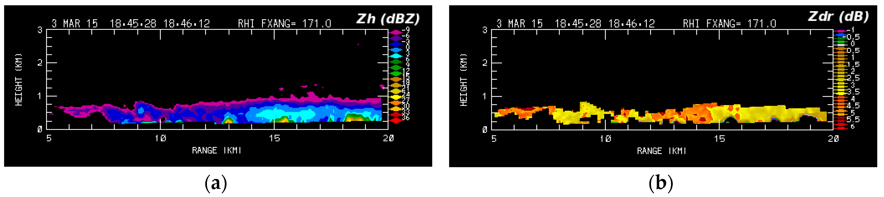
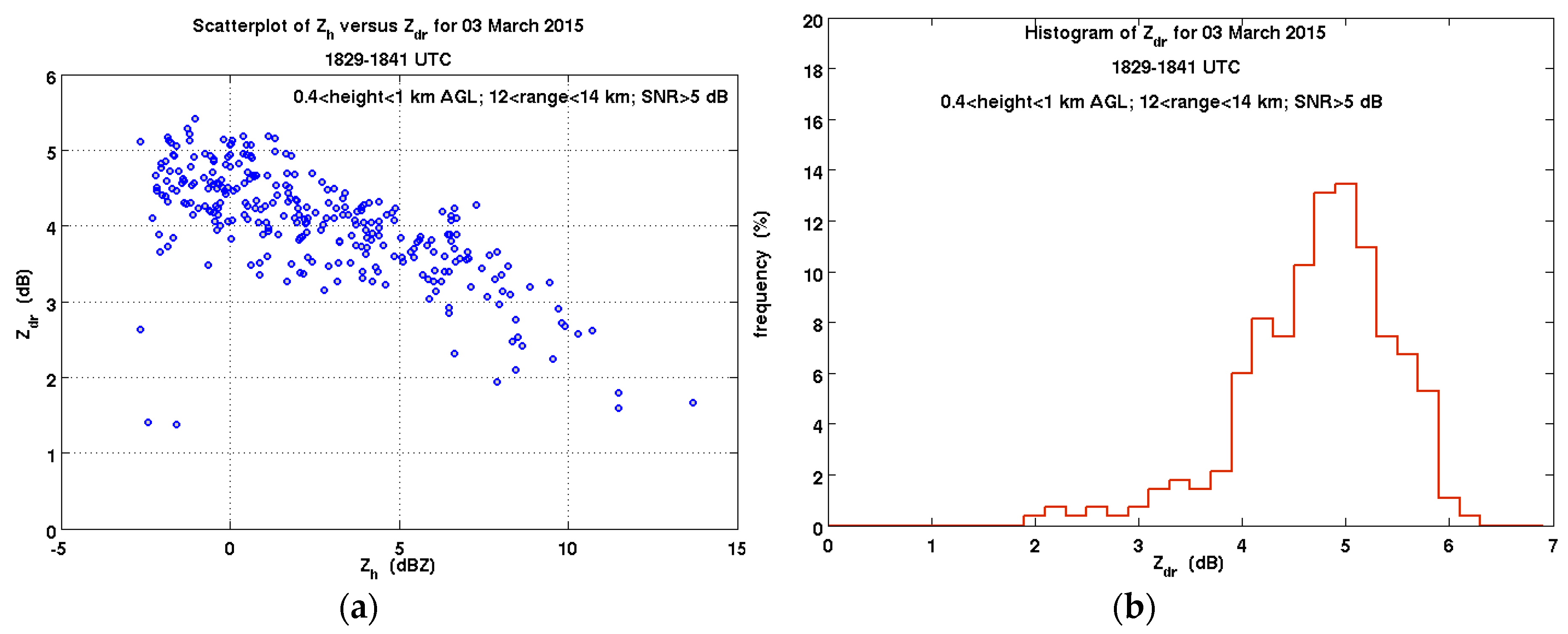
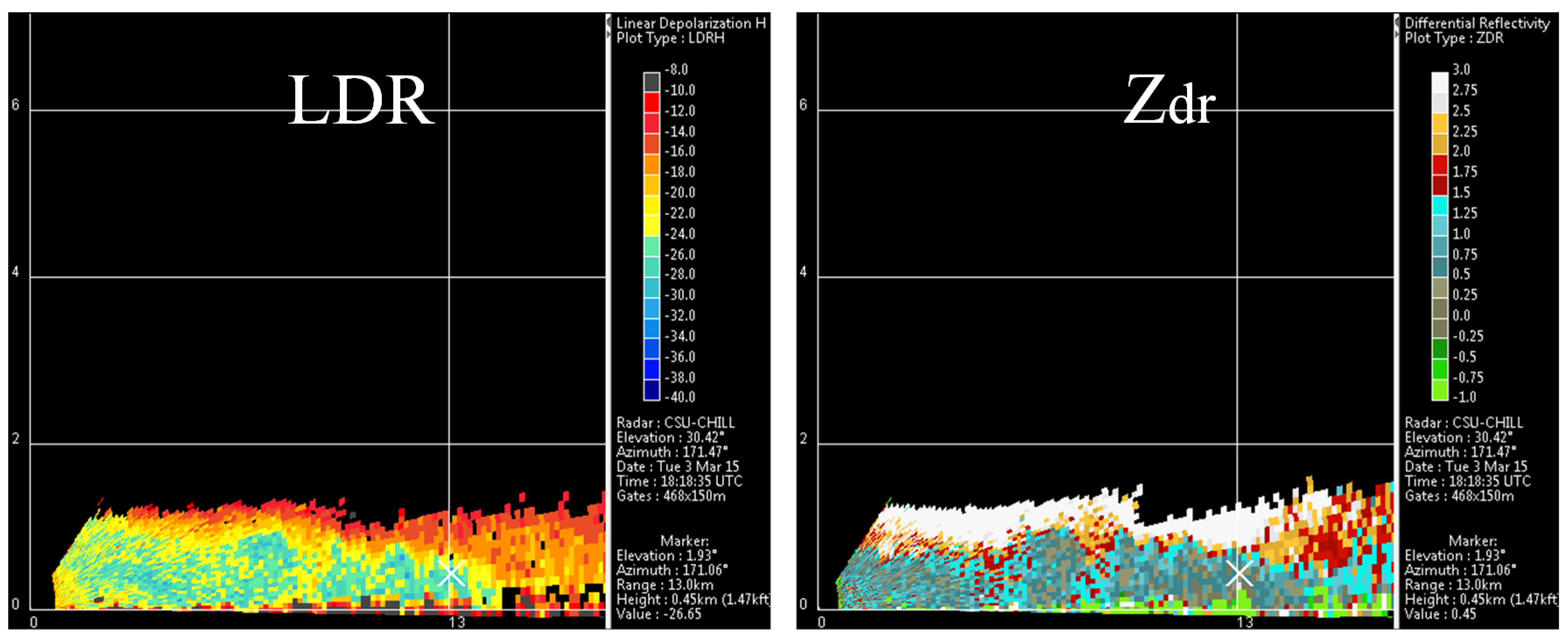
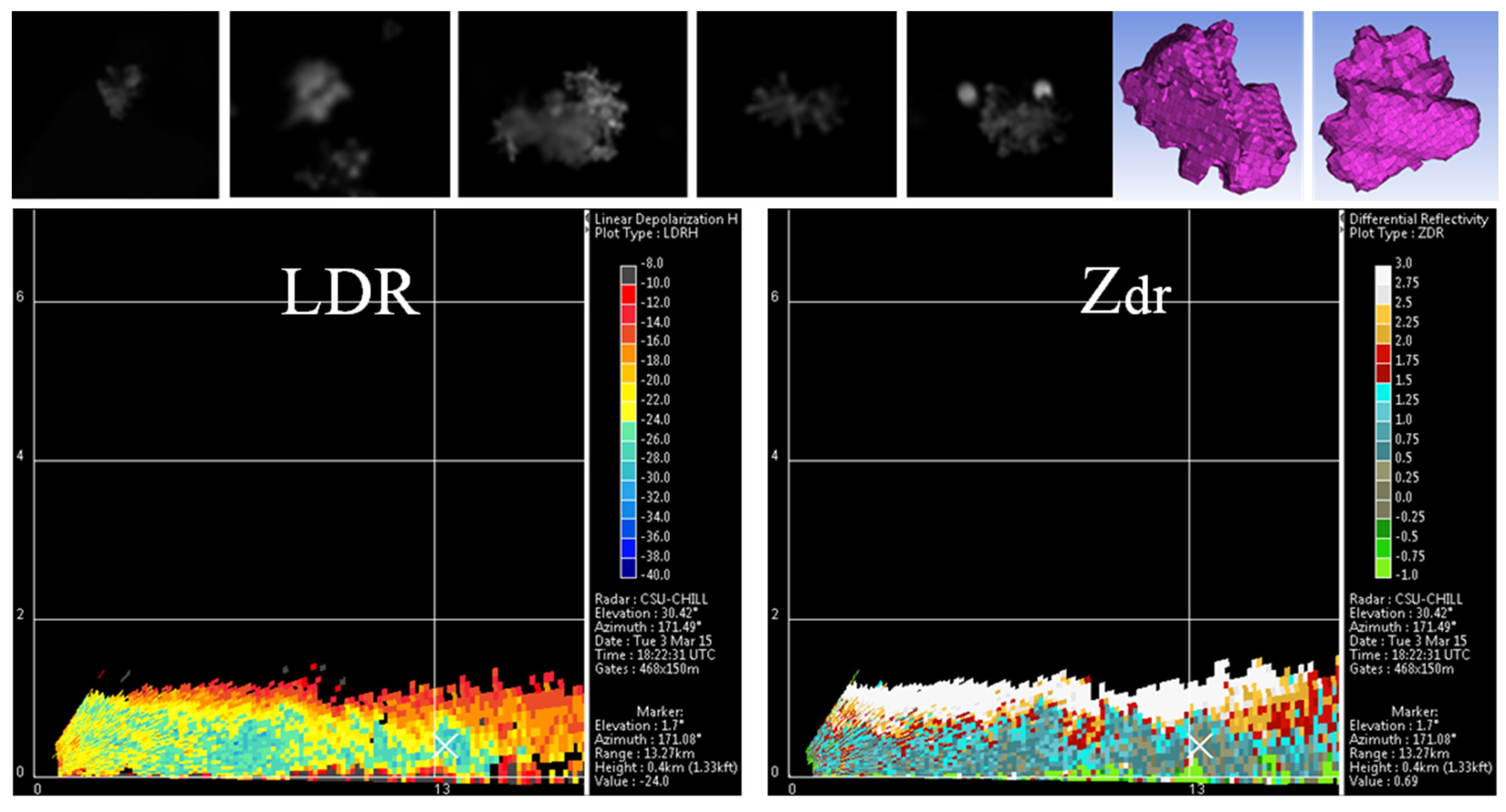
The article has also described the MASCRAD project and the 2014/2015 MASCRAD winter campaign, and has presented and discussed selected illustrative observation data, results, and analyses for three cases with widely-differing meteorological settings that involved contrasting hydrometeor forms, namely, an unusual winter graupel shower event on 16 February 2015, a major snow band passage event on 21–22 February 2015, and a positive Z_dr in a dissipating light snow event on 3 March 2015. Illustrative results of scattering calculations based on MASC images captured during these events, along with initial comparison with radar data. Selected comparative studies of snow habits from MASC, 2DVD, and CHILL radar data have also been presented, along with the analysis of microphysical characteristics of particles. In addition, a link between the vertical structure of precipitation, obtained from the CSU-CHILL radar, and the snow characteristics at ground level, using the 2DVD and MASC data, has been analyzed and discussed for the 21–22 February 2015 heavy snowfall case.

This newly developed framework has potential to advance frozen phase precipitation remote sensing and microphysics research. Through judicious use of these technologies, many ongoing and emerging observational and modeling activities can be enhanced. Ongoing and future work using this approach includes a variety of aspects relevant to the broader remote sensing and microphysics communities, and may also spur future collaborative efforts.

References

1. Pruppacher, H.R.; Klett, J.D. Microphysics of clouds and precipitation. In Series: Atmospheric and Oceanographic Sciences Library, 2nd ed.; Springer: Berlin/Heidelberg, Germany, 2010; Volume 18. [Google Scholar]
2. Mason, B.J. The Physics of Clouds; Oxford University Press: Oxford, UK, 2010. [Google Scholar]
3. Straka, J.; Zrnić, D.S.; Ryzhkov, A.V. Bulk hydrometeor classification and quantification using polarimetric radar data: Synthesis of Relations. J. Appl. Meteorol. 2000, 39, 1341–1372. [Google Scholar] [CrossRef]
4. Matrosov, S.Y.; Reinking, R.F.; Kropfli, R.A.; Martner, B.E.; Bartram, B.W. On the use of radar depolarization ratios for estimating shapes of ice hydrometeors in winter clouds. J. Appl. Meteorol. 2001, 40, 479–490. [Google Scholar] [CrossRef]
5. Zhang, G.; Luchs, S.; Ryzhkov, A.; Xue, M.; Ryzhkova, L.; Cao, Q. Winter precipitation microphysics characterized by polarimetric radar and video disdrometer observations in central Oklahoma. J. Appl. Meteorol. Climatol. 2011, 50, 1558–1570. [Google Scholar] [CrossRef]
6. Tyynelä, J.; Leinonen, J.; Moisseev, D.; Nousiainen, T. Radar backscattering from snowflakes: Comparison of fractal, aggregate, and soft spheroid models. J. Atmos. Ocean. Technol. 2011, 28, 1365–1372. [Google Scholar] [CrossRef]
7. Vivekanandan, J.; Bringi, V.N.; Hagen, M.; Meischner, P. Polarimetric radar studies of atmospheric ice particles. IEEE Trans. Geosci. Remote Sens. 1994, 32, 1–10. [Google Scholar] [CrossRef]
8. Reinking, R.F.; Matrosov, S.Y.; Kropfli, R.A.; Bartram, B.W. Evaluation of a 45° slant quasi-linear radar polarization state for distinguishing drizzle droplets, pristine ice crystals, and less regular ice particles. J. Atmos. Ocean. Technol. 2002, 19, 296–321. [Google Scholar] [CrossRef]
9. Kennedy, P.C.; Rutledge, S.A. S-band dual-polarization radar observations of winter storms. J. Appl. Meteorol. Climatol. 2011, 50, 844–858. [Google Scholar] [CrossRef]
10. Andrić, J.; Kumjian, M.R.; Zrnić, D.S.; Straka, J.M.; Melnikov, V.M. Polarimetric signatures above the melting layer in winter storms: An observational and modeling study. J. Appl. Meteorol. Climatol. 2013, 52, 682–700. [Google Scholar] [CrossRef]
11. Ryzhkov, A.V.; Zrnic, D.S.; Gordon, B.A. Polarimetric method for ice water content determination. J. Appl. Meteorol. 1998, 37, 125–134. [Google Scholar] [CrossRef]
12. Barthazy, E.; Göke, S.; Schefold, R.; Högl, D. An optical array instrument for shape and fall velocity measurements of hydrometeors. J. Atmos. Ocean. Technol. 2004, 21, 1400–1416. [Google Scholar] [CrossRef]
13. Schönhuber, M.; Lammer, G.; Randeu, W.L. The 2D-video-distrometer. In Precipitation: Advances in Measurement, Estimation and Prediction; Silas, M., Ed.; Springer: Berlin/Heidelberg, Germany, 2008. [Google Scholar]
14. Szyrmer, W.; Zawadzki, I. Snow studies. Part II: Average relationship between mass of snowflakes and their terminal fall velocity. J. Atmos. Sci. 2010, 67, 3319–3335. [Google Scholar] [CrossRef]
15. Huang, G.-J.; Bringi, V.N.; Petersen, W.A.; Carey, L.; Schultz, C.J.; Gatlin, P.N. Case studies of winter precipitation events using 2D-video disdrometers and c-band radar. In Proceedings of the 35th Conference on Radar Meteorology, Pittsburgh, PA, USA, 26–30 September 2011.
16. Huang, G.-J.; Bringi, V.N.; Cifelli, R.; Hudak, D.; Petersen, W.A. A methodology to derive radar reflectivity–liquid equivalent snow rate relations using C-band radar and a 2D video disdrometer. J. Atmos. Ocean. Technol. 2010, 27, 637–651. [Google Scholar] [CrossRef]
17. Böhm, H.P. A general equation for the terminal fall speed of solid hydrometeors. J. Atmos. Sci. 1989, 46, 2419–2427. [Google Scholar] [CrossRef]
18. Heymsfield, A.J.; Westbrook, C.D. Advances in the estimation of ice particle fall speeds using laboratory and field measurements. J. Atmos. Sci. 2010, 67, 2469–2482. [Google Scholar] [CrossRef]
19. Zrnić, D.S.; Ryzhkov, A.; Straka, J.; Liu, Y.; Vivekanandan, J. Testing a procedure for automatic classification of hydrometeor types. J. Atmos. Ocean. Technol. 2001, 18, 892–913. [Google Scholar] [CrossRef]
20. Giangrande, S.E.; Ryzhkov, A.V. Estimation of rainfall based on the results of polarimetric echo classification. J. Appl. Meteorol. Climatol. 2008, 47, 2445–2462. [Google Scholar] [CrossRef]
21. Mishchenko, M.I.; Travis, L.D.; Lacis, A.A. Scattering, Absorption, and Emission of Light by Small Particles; Cambridge University Press: Cambridge, UK, 2002. [Google Scholar]
22. Draine, B.T.; Flatau, P.J. Discrete-dipole approximation for scattering calculations. J. Opt. Soc. Am. A 1994, 11, 1491–1499. [Google Scholar] [CrossRef]
23. Notaros, B.; Bringi, V.N.; Kleinkort, C.; Huang, G.-J.; Chobanyan, E.; Thurai, M.; Notaros, O.; Manic, A.; Newman, A.; Kennedy, P.; et al. Measurement and characterization of winter precipitation at MASCRAD snow field site. In Proceedings of the 2015 IEEE International Symposium on Antennas and Propagation and North American Radio Science Meeting, Vancouver, BC, Canada, 19–24 July 2015; pp. 979–980.
24. Notaros, B.M.; Bringi, V.N.; Newman, A.J.; Kleinkort, C.; Huang, G.-J.; Kennedy, P.; Thurai, M. Accurate characterization of winter precipitation using in-situ instrumentation, CSU-chill radar, and advanced scattering methods. In Proceedings of the 2015 AGU Fall Meeting, San Francisco, CA, USA, 14–18 December 2015.
25. Kleinkort, C.; Huang, G.-J.; Chobanyan, E.; Manic, A.; Ilic, M.; Pezeshki, A.; Bringi, V.N.; Notaros, B. Visual hull method based shape reconstruction of snowflakes from MASC photographs. In Proceedings of the 2015 IEEE International Symposium on Antennas and Propagation and North American Radio Science Meeting, Vancouver, BC, Canada, 19–25 July 2015; pp. 1122–1123.
26. Kleinkort, C.; Huang, G.-J.; Manic, S.; Manic, A.; Kennedy, P.; Hubbert, J.; Newman, A.; Bringi, V.N.; Notaros, B. 3D shape reconstruction of snowflakes from multiple images, meshing, dielectric constant estimation, scattering analysis, and validation by radar measurements. In Proceedings of the American Meteorological Society’s 37th Conference on Radar Meteorology, Norman, OK, USA, 14–18 September 2015.
27. Chobanyan, E.; Sekeljiic, N.J.; Manic, A.B.; Ilic, M.M.; Bringi, V.N.; Notaros, B.M. Efficient and accurate computational electromagnetics approach to precipitation particle scattering analysis based on higher order method of moments integral-equation modeling. J. Atmos. Ocean. Technol. 2015, 32, 1745–1758. [Google Scholar] [CrossRef]
28. Kennedy, P.C.; Kleinkort, C.; Huang, G.-J.; Thurai, M.; Newman, A.; Hubbert, J.; Rutledge, S.; Bringi, V.N.; Notaros, B.M. Preliminary results from the multi-angle snowflake camera and radar (MASCRAD) project. In Proceedings of the American Meteorological Society’s 37th Conference on Radar Meteorology, Norman, OK, USA, 14–18 September 2015.
29. Bringi, V.N.; Notaros, B.; Kleinkort, C.; Huang, G.-J.; Thurai, M.; Kennedy, P. Comprehensive analysis of an unusual winter graupel shower event recorded by an S-band polarimetric radar and two optical imaging surface instruments. In Proceedings of the American Meteorological Society’s 37th Conference on Radar Meteorology, Norman, OK, USA, 14–18 September 2015.
30. Notaros, B.M.; Bringi, V.N.; Chobanyan, E.; Kleinkort, C.; Manic, S.B.; Sekeljic, N.J.; Manic, A.B.; Ilic, M.M. Computation of particle scattering matrices and polarimetric radar variables for winter precipitation using T-matrix method, DDA method, and higher order MoM-SIE method. In Proceedings of the American Meteorological Society’s 37th Conference on Radar Meteorology, Norman, OK, USA, 14–18 September 2015.
31. Garrett, T.J.; Fallgatter, C.; Shkurko, K.; Howlett, D. Fallspeed measurement and high-resolution multi-angle photography of hydrometeors in freefall. Atmos. Meas. Tech. Discuss. 2012, 5, 4827–4850. [Google Scholar] [CrossRef]
32. Svoboda, T.; Martinec, D.; Pajdla, T. A convenient multi-camera self-calibration for virtual environments. Presence 2005, 14, 407–422. [Google Scholar] [CrossRef]
33. Laurentini, A. The visual hull concept for silhouette-based image understanding. IEEE Trans. Pattern Anal. Mach. Intell. 1994, 16, 150–162. [Google Scholar] [CrossRef]
34. Laurentini, A. How far 3D shapes can be understood from 2D Silhouettes. IEEE Trans. Pattern Anal. Mach. Intell. 1995, 17, 188–195. [Google Scholar] [CrossRef]
35. Baumgart, B.G. Geometric Modeling for Computer Vision. Ph.D. Thesis, Computer Science Department, Stanford University, Stanford, CA, USA, 1974. [Google Scholar]
36. Matusik, W.; Buehler, C.; Raskar, R.; McMillan, L.; Gortler, S. Image-based visual hulls. In Proceedings of the 27th Annual Conference on Computer Graphics and Interactive Techniques, New Orleans, LA, USA, 23–28 July, 2000; pp. 369–374.
37. Forbes, K. Calibration, Recognition, and Shape from Silhouettes of Stones. Ph.D. Thesis, Department of Electrical Engineering, University of Cape Town, Cape Town, South Africa, 2007. [Google Scholar]
38. VHMC Software: Visual Hull Mesh Code. 2012. Available online: http://www.dip.ee.uct.ac.za/~kforbes/DoubleMirror/DoubleMirror.html (accessed on 3 June 2016).
39. Teschl, F. Scattering of Millimeter and Centimeter Radio Waves by Solid Precipitation Particles. Ph.D. Thesis, Institute of Broadband Communications, Graz University of Technology, Graz, Austria, 2005. [Google Scholar]
40. Teschl, F.; Randeu, W.L.; Schönhuber, M. Modelling microwave scattering by solid precipitation particles. In Proceedings of the European Conference on Antennas and Propagation (EuCAP 2006), Nice, France, 6–10 November 2006.
41. Huang, G.-J.; Bringi, V.N.; Moisseev, D.; Petersen, W.A.; Bliven, L.; Hudak, D. Use of 2D-video disdrometer to derive mean density–size and Ze–SR relations: Four snow cases from the light precipitation validation experiment. Atmos. Res. 2014, 153, 34–48. [Google Scholar] [CrossRef]
42. ANSYS ICEM CFD. 2014. Available online: http://resource.ansys.com/Products/Other+Products/ANSYS+ICEM+CFD (accessed on 3 June 2016).
43. Schönhuber, M.; Urban, H.E.; Randeu, W.L.; Poiares Baptista, J.P.V. Distrometer results obtained in various climates and their application to weather radar data inversion. In Proceedings of the ESA SP-444 Proceedings, Millennium Conference on Antennas & Propagation, Davos, Switzerland, 9–14 April 2000.
44. Hanesch, M. Fall Velocity and Shape of Snowflakes. Ph.D. Thesis, Swiss Federal Institute of Technology, Zurich, Switzerland, 1999. [Google Scholar]
45. Brandes, E.A.; Ikeda, K.; Zhang, G.; Schonhuber, M.; Rasmussen, R.M. A statistical and physical description of hydrometeor distributions in Colorado snowstorms using a video disdrometer. J. Appl. Meteorol. Climatol. 2007, 46, 634–650. [Google Scholar] [CrossRef]
46. Kruger, A.; Krajewski, W.F. Two-Dimensional Video Disdrometer: A Description. J. Atmos. Ocean. Technol. 2002, 19, 602–617. [Google Scholar] [CrossRef]
47. Kleinkort, C.; Huang, G.-J.; Bringi, V.N.; Notaros, B.M. Polarimetric scattering analysis of snow and ice particles using field measurements by 2D-video disdrometer. In Proceedings of the 2015 USNC-URSI Radio Science Meeting (Joint with AP-S Symposium), Vancouver, BC, Canada, 19–24 July 2015; p. 287.
48. Rasmussen, R.; Baker, B.; Kochendorfer, J.; Meyers, T.; Landolt, S.; Fischer, A.P.; Black, J.; Thériault, J.M.; Kucera, P.; Gochis, D.; et al. How well are we measuring snow: The NOAA/FAA/NCAR winter precipitation test bed? Bull. Am. Meteorol. Soc. 2012, 93, 811–829. [Google Scholar] [CrossRef]
49. Hubbert, J.C.; Kennedy, P.; Chandrasekar, V.; Rutledge, S.; Lee, W.C.; Bringi, V.N.; Wilson, J.; Brunkow, D.; Dixon, M.; Weckwerth, T.; et al. FRONT: The front range observational network testbed. In Proceedings of 92nd AMS Annual Meeting, New Orleans, LA, USA, 22–26 January 2012.
50. Bringi, V.N.; Hoferer, R.; Brunkow, D.A.; Schwerdtfeger, R.; Chandrasekar, V.; Rutledge, S.A.; George, J.; Kennedy, P.C. Design and performance characteristics of the new 8.5-m dual-offset gregorian antenna for the CSU–CHILL radar. J. Atmos. Ocean. Technol. 2011, 28, 907–920. [Google Scholar] [CrossRef]
51. Zrnić, D.; Doviak, R.; Zhang, G.; Ryzhkov, A. Bias in differential reflectivity due to cross coupling through the radiation patterns of polarimetric weather radars. J. Atmos. Ocean. Technol. 2010, 27, 1624–1637. [Google Scholar] [CrossRef]
52. Hubbert, J.C.; Ellis, S.M.; Dixon, M.; Meymaris, G. Modeling, error analysis, and evaluation of dual-polarization variables obtained from simultaneous horizontal and vertical polarization transmit radar. Part II: Experimental data. J. Atmos. Ocean. Technol. 2010, 27, 1599–1607. [Google Scholar]
53. Ryzhkov, A.V.; Zrnić, D.S. Depolarization in ice crystals and its effect on radar polarimetric measurements. J. Atmos. Ocean. Technol. 2007, 24, 1256–1267. [Google Scholar] [CrossRef]
54. Hendry, A.; Antar, Y.M.M. Precipitation particle identification with centimeter wavelength dual-polarization radars. Radio Sci. 1984, 19, 115–122. [Google Scholar] [CrossRef]
55. Höller, H.; Bringi, V.N.; Hubbert, J.; Hagen, M.; Meischner, P.F. Life cycle and precipitation formation in a hybrid-type hailstorm revealed by polarimetric and Doppler radar measurements. J. Atmos. Sci. 1994, 51, 2500–2522. [Google Scholar] [CrossRef]
56. Evaristo, R.; Bals-Esholz, T.; Williams, E.; Fenn, A.J.; Donovan, M.; Smalley, D. Relationship of graupel shape to differential reflectivity: Theory and observations. In Proceedings of the AMS 29th Conference on Environmental Information Processing, Austin, TX, USA, 6–10 January 2013.
57. Lee, J.E.; Jung, S.H.; Park, H.M.; Kwon, S.; Lin, P.L.; Lee, G. Classification of precipitation types using fall velocity-diameter relationships from 2D-video distrometer measurements. Adv. Atmos. Sci. 2015, 32, 1277–1290. [Google Scholar] [CrossRef]
58. Mosimann, L. An improved method for determining the degree of snow crystal riming by vertical Doppler radar. Atmos. Res. 1995, 37, 305–323. [Google Scholar] [CrossRef]
59. Kumjian, M.R.; Rutledge, S.A.; Rasmussen, R.M.; Kennedy, P.C.; Dixon, M. High-resolution polarimetric radar observations of snow-generating cells. J. Appl. Meteorol. Climatol. 2014, 53, 1636–1658. [Google Scholar] [CrossRef]
60. Ono, A. The shape and riming properties of ice crystals in natural clouds. J. Atmos. Sci. 1969, 26, 138–147. [Google Scholar] [CrossRef]
Figure 1. Multi-Angle Snowflake Camera (MASC): (a) photograph showing three cameras and electronic and mechanical components; (b) 3D schematic showing basic components (the “hatched” area represents the cross section for triggering of the near-IR motion detection system); (c) planar view of the prototype design with cameras having equal horizontal field of views (FOVs) and depth of fields (DOFs); and (d) precisely defined virtual measurement area (yellow-colored area); (e,f) Adding two “external” cameras, in temperature controlled enclosures, to the Colorado State University (CSU) MASC, to improve 3D reconstruction of snowflakes.
Atmosphere 07 00081 g001
Figure 2. Characteristic examples of images of snowflakes with contrasting forms collected by the MASC (Figure 1) at the MASC + Radar (MASCRAD) field Site during the 2014/2015 MASCRAD winter campaign.
Atmosphere 07 00081 g002
Figure 3. Illustration of MASC-VHMC snowflake measurement-reconstruction: (a) visual hull (VHMC) reconstruction of the 3D shape of a snowflake based on MASC (Figure 1) photographs and the corresponding 2D silhouettes of the object; (b) triangular 3D mesh of the reconstructed snowflake; (c,d) MASC photograph and corresponding projection of the VHMC-generated 3D mesh in (b) to the camera image plane in (a) for the first camera; (e,f) MASC photograph and mesh projection for the second camera; (g,h) photograph and projection for the third camera.
Atmosphere 07 00081 g003
Figure 4. Two sets, (a) and (b), of five images of two snowflakes collected by five cameras of the new five-camera MASC system during the snow storm on 15 November 2014, at the MASCRAD Field Site. In each horizontal panel, (a) or (b), images 1–3 are taken by the three original “internal” MASC cameras, while images 4–5 are taken by the two additional “external” cameras of much lower resolution (but sufficient for the visual hull 3D shape reconstruction method).
Atmosphere 07 00081 g004
Figure 5. An example of snowflake reconstruction by the visual hull method based on five photographs of a snowflake collected by the new 5-camera CSU MASC system in Figure 1e: (a) MASC images and corresponding projections of the visual hull generated 3D mesh to camera image planes and (b) the resulting triangular 3D mesh of the snowflake.
Atmosphere 07 00081 g005
Figure 6. Examples of 3D shape reconstruction of snow particles from three high-resolution MASC photographs using the visual hull (VH) image processing method (VHMC) and ANSYS ICEM CFD meshing software: recorded MASC images and 3D reconstructed shapes (in the form of meshes of quadrilateral patches suitable for method of moments (MoM) surface integral equation (SIE) scattering modeling) for (a) and (b) a snow aggregate, (c) and (d) a mostly rimed graupel.
Atmosphere 07 00081 g006
Figure 7. Example of re-meshing of the visual hull output: (a) triangular patch representation; (b) coarse quadrilateral patch representation; and (c) refined quadrilateral patch representation.
Atmosphere 07 00081 g007
Figure 8. (a) Two-dimensional video disdrometer (2DVD), SN36 model; (b) Schematic showing the geometry of the 2DVD; from [46]. Details of the instrument can be found in [13].
Atmosphere 07 00081 g008
Figure 9. A 2DVD installed next to the MASC within the same wind fence at the MASCRAD instrumentation site.
Atmosphere 07 00081 g009
Figure 10. Particle collection comparison between the MASC and the 2DVD (in Figure 9) for selected events during the MASCRAD 2014/2015 snow season. Note that the ratio of sampling areas of the 2DVD and the MASC is ~3 (approximately 3 cm × 10 cm for the MASC and 10 cm × 10 cm for the 2DVD).
Atmosphere 07 00081 g010
Figure 11. Generalized curved parametric quadrilateral patch, with r(u,v) defined in Equation (1) and the square parent domain also shown, for higher order MoM-SIE modeling of winter precipitation particles. Element currents are modeled by polynomial basis functions of arbitrary orders, as in Equation (1).
Atmosphere 07 00081 g011
Figure 12. (a) Definition of cross-sectional areas Ae (the shadowed area) and A (the area of the smallest ellipse completely containing Ae—it includes Ae and the hatched area) presented to the flow; from [17]; (b) Bottom view (normal to the flow) automatically obtained from the reconstructed 3D shape of a snow particle using the visual hull method.
Atmosphere 07 00081 g012
Figure 13. (a) Two best candidate sites for the MASCRAD project: the “Nesse site” and the “Easton site”, at a range of 14.88 km and 12.92 km, respectively, from the CHILL Radar; (b) From the Easton Valley View Airport, one can see the CHILL Radar radome.
Atmosphere 07 00081 g013
Figure 14. Nesse site (at a range of 14.88 km) as rain approached on 27 August 2014: VCHILL (Virtual CHILL) displays of (a) Ze and (b) LDR measured by CSU-CHILL Radar. LDR “wedge” is apparent, due to the University of Northern Colorado/Greeley hill, downrange; it fades out as precipitation echo strength exceeds about 25 dBZ.
Atmosphere 07 00081 g014
Figure 15. Easton site (12.92 km range) with ~30 dBZ rain: CSU-CHILL Radar measurements of (a) Ze and (b) LDR. LDR looks reasonable down to near-surface elevations. It appeared that reasonable LDR can be obtained down to lower reflectivity levels at the Easton site versus the Nesse site (Figure 14).
Atmosphere 07 00081 g015
Figure 16. MASCRAD Snow Field Site at Easton Valley View Airport, Colorado: (a) 2/3-scaled DFIR double wind fence right after construction in October 2014 and (b) 2DVD, VAISALA, and MASC instruments operating within the DFIR fence.
Atmosphere 07 00081 g016
Figure 17. Plots of the GAUS measured wind speed data on 2 and 3 December 2014 at the MASCRAD Snow Field Site: (a) surface data outside the wind fence (surrounding environment) and (b) surface data inside the wind fence (distrometer environment)—both measured by NCAR Mesonet sensors.
Atmosphere 07 00081 g017
Figure 18. (a) The Front Range Observational Network Testbed (FRONT) [49] map showing location of various radars; (b) MASCRAD Easton Field Site is located about 12.92 km south/southeast of the CSU-CHILL Radar, along the baseline to the SPOL Radar.
Atmosphere 07 00081 g018
Figure 19. CSU-CHILL 3.0° elevation angle PPI horizontal reflectivity, Zh, data (in dBZ) at 18:24 UTC on 16 February 2015. These initial echoes developed approximately 10 km south of the MASCRAD Field Site and moved southward. Similar small convective echoes passed the Easton site approximately one hour later.
Atmosphere 07 00081 g019
Figure 20. Range-height indicator (RHI) scan through a convective echo near the Easton site (12.92 km range) at 19:27 UTC on 16 February 2015. (a) Horizontal reflectivity, Zh, in dBZ; (b) Differential reflectivity, Zdr, in dB. Horizontal ranges and heights (AGL) are in km.
Atmosphere 07 00081 g020
Figure 21. Example MASC images recorded during the 16 February 2015 graupel showers at the MASCRAD Easton site.
Atmosphere 07 00081 g021
Figure 22. Illustrative results of MoM-SIE scattering calculations based on the MASC images captured at the MASCRAD Field Site during the unusual winter graupel shower event on 16 February 2015 and the resulting 3D shape reconstruction, in comparison with the corresponding CSU-CHILL radar RHI plots of LDR and Zdr at the same time. Results: MASC/MoM-SIE: εr = 1.275 − j0.0003, LDR = −36 dB, Zdr = −0.15 dB; CHILL Radar: LDR = −35 dB, Zdr = −0.21 dB, at the 12.92-km range.
Atmosphere 07 00081 g022
Figure 23. Some more illustrative results of MoM-SIE scattering calculations based on the MASC images captured during the 16 February 2015 event, in comparison with CSU-CHILL radar RHI plots at the same time. Results: MASC/MoM-SIE: εr = 1.19 − j0.0002, LDR = −24.5 dB, Zdr = −0.05 dB; CHILL Radar: LDR = −33 dB, Zdr = −0.02 dB (12.92-km range).
Atmosphere 07 00081 g023
Figure 24. SPOL radar reflectivity data collected in a 0.8° plan position indicator (PPI) scan as a major snow band arrived at the CSU-CHILL radar site at 20:51 UTC on 21 February 2015. Axes are in km from SPOL.
Atmosphere 07 00081 g024
Figure 25. CSU-CHILL radar RHI scan over the MASCRAD Easton site (located at a range of 12.92 km) at ~21:31 UTC on 21 February 2015. (a) Maximum reflectivities slightly exceeded 30 dBZ; (b) Differential reflectivities were near 0 dB in the high reflectivity regions.
Atmosphere 07 00081 g025
Figure 26. Selected MASC images starting at 21:41 UTC on 21 February 2015.
Atmosphere 07 00081 g026
Figure 27. Differential reflectivity (Zdr) histograms for the 16 February 2015 graupel and 21 February 2015 snow band cases.
Atmosphere 07 00081 g027
Figure 28. Linear depolarization ratio (LDR) histograms for the graupel and snow band cases.
Atmosphere 07 00081 g028
Figure 29. (a) RHI scan display from the CSU-CHILL radar at 21:30 UTC on 21 February 2015; (b) Horizontal reflectivity, Zh, height-time indicator above the MASCRAD Field Site, extracted from RHI scans during the 21–22 February 2015 event; (c) Differential reflectivity, Zdr, height-time indicator for the event; blue and black circles indicate negative Zdr and high Zdr (Zdr > 3 dB) regions, respectively.
Atmosphere 07 00081 g029aAtmosphere 07 00081 g029b
Figure 30. Scatterplots of (a) linked ∇Zh versus Dm and (b) linked ∇Zh versus Nw for the 21–22 February 2015 event. Solid lines and the corresponding linear relations ∇Zh(Dm) and ∇Zh(Nw) given in the figure represent the least-squares fitting results.
Atmosphere 07 00081 g030
Figure 31. Time series of (a) the particle size distribution (PSD) and (b) the particle velocity distribution for the 21–22 February 2015 event, with representative MASC images also shown.
Atmosphere 07 00081 g031
Figure 32. Illustrative results of MoM-SIE scattering calculations based on the MASC images captured at the MASCRAD Field Site during the major snow band passage event on 21 February 2015 and the resulting 3D shape reconstruction, in comparison with the corresponding CSU-CHILL radar RHI plots of LDR and Zdr at the same time. Results: MASC/MoM-SIE: εr = 1.216 − j0.0002, LDR = −31 dB, Zdr = −0.1 dB; CHILL Radar: LDR = −29 dB, Zdr = −0.17 dB, at the 12.92-km range.
Atmosphere 07 00081 g032
Figure 33. Some more illustrative results of MoM-SIE scattering calculations based on the MASC images captured during the 21 February 2015 event, in comparison with CSU-CHILL radar data (12.92-km range). Results: MASC/MoM-SIE: εr = 1.201 − j0.0002, LDR = −31.5 dB, Zdr = −0.48 dB; CHILL Radar: LDR = −32 dB, Zdr = −0.12 dB.
Atmosphere 07 00081 g033aAtmosphere 07 00081 g033b
Figure 34. (a) Horizontal reflectivity and (b) differential reflectivity in an RHI scan over the MASCRAD Easton site at 18:45 UTC on 3 March 2015.
Atmosphere 07 00081 g034
Figure 35. (a) Zh vs. Zdr scatterplot and (b) Zdr histogram for 18:29–18:41 UTC on 3 March 2015 in the immediate Easton area.
Atmosphere 07 00081 g035
Figure 36. Selected MASC images between 18:33 and 18:38 UTC on 3 March 2015.
Atmosphere 07 00081 g036
Figure 37. Illustrative results of MoM-SIE scattering calculations based on the MASC images captured at the MASCRAD Field Site during the positive Zdr in dissipating light snow area event on 3 March 2015 and the resulting 3D shape reconstruction, in comparison with the corresponding LDR and Zdr data observed simultaneously by the CSU-CHILL radar. Results: MASC/MoM-SIE: εr = 1.153 − j0.0002, LDR = −36 dB, Zdr = 0.28 dB; CHILL Radar: LDR = −27 dB, Zdr = 0.45 dB, at the 12.92-km range.
Atmosphere 07 00081 g037aAtmosphere 07 00081 g037b
Figure 38. Some more illustrative results of MASC/MoM-SIE calculations for the 3 March 2015 event, in comparison with CSU-CHILL radar data (12.92-km range). Results: MASC/MoM-SIE: εr = 1.122 − j0.0003, LDR = −19.5 dB, Zdr = 0.18 dB; CHILL Radar: LDR = −24 dB, Zdr = 0.7 dB.
Atmosphere 07 00081 g038