Article

A Geostatistics-Based Method to Determine the Pixel Distance in a Structure Function Model for Aerosol Optical Depth Inversion

1
School of Instrumentation Science and Opto-electronics Engineering, Beihang University, No. 37 Xueyuan RD, Beijing 100191, China
2
Key Laboratory of Space Ocean Remote Sensing and Application, SOA, Beijing 100081, China
3
State Key Laboratory of Remote Sensing Science, Institute of Remote Sensing and Digital Earth, Chinese Academy of Sciences, Beijing 100094, China
4
State Key Laboratory of Environmental Criteria and Risk Assessment, Chinese Research Academy of Environmental Sciences, Beijing 10012, China
5
School of Transportation Science and Engineering, Beihang University, No. 37 Xueyuan RD, Beijing 100191, China
*
Authors to whom correspondence should be addressed.
Atmosphere 2017, 8(1), 6; https://doi.org/10.3390/atmos8010006
Submission received: 23 November 2016 / Revised: 26 December 2016 / Accepted: 4 January 2017 / Published: 10 January 2017

Abstract

:
Inversion of aerosol optical depth (AOD) over bright land surface by optical remote sensing is particularly challenging because surface reflectance dominates the satellite signal. A structure function method is suitable and can effectively solve aerosol optical depth inversion in high reflectance areas. How to select d (the pixel distance between two pixels) value is one of the key problems with the structure function method. We present a method based on geostatistics, where variogram theory is referenced, to determine the pixel distance in structure function model for aerosol optical depth inversion. This method was validated by the Moderate Resolution Imaging Spectroradiometer (MODIS) 1 km resolution level 1B data from Beijing, China. The results indicate that the relationship between variogram and d in four different directions can be fitted by exponential function, of which correlation coefficients are all above 0.9. Compared with the MODIS aerosol product (MOD 04 product), the inversion AOD has higher accuracy, with an absolute error of −0.00187 instead of −0.00854 and a relative error of 0.99% instead of 4.35%, based on AERosol RObotic NETwork (AERONET) observations. For validation, we applied this new method separately to both Beijing–Tianjin–Hebei region and MODIS 500 m resolution images for region and resolution validation. The results show that inversion AOD has higher accuracy and more efficient pixels.

1. Introduction

Atmospheric aerosols are important components in the Earth system [1] and play an important role in climate [2], air quality [3], and human health [4] research through direct and indirect radiation forcing [5,6]. The inversion methods in aerosol remote sensing have been extensively studied, and much improvement has been made in recent decades [7]. However, aerosol information is hard to identify in high reflectance areas because the radiation acquired by satellites mainly comes from the surface contribution [8], therefore the inversion of aerosol optical depth (AOD) is particularly challenging in areas of high reflectance [9]. However, the structure function method is quite limited in application. Huang et al. [10] pointed out that for a wide range of homogeneous surface, the structure function value is small, so the small error of structure function between the images of two days will cause greater errors in inversion results. Nevertheless, a great deal of work has been undertaken to promote the application of the structure function method. One key problem is how to determine the d value aside from selecting a surface with a clear structure of where there are obvious reflectivity changes. Tanré et al. [11] pointed out that the rule structure function value becomes larger with the increase of d, and then remains stable. The structure function value in a single direction is determined by its slope height. However, they chose sea surface zones as a comparison to calculate the structure function value. These zones were chosen a few kilometers apart from the coast in the scene, which means that the magnitude of structure function value was zero, and even reached one. Holben et al. [12] found that the change of structure function value with d was not regular because of the impact of terrain and observation geometry. Therefore they put forward a compared structure function model in three directions, and used the mean d value method from 1 to 10 to retrieve AOD. Lin et al. [13] applied the improved multi direction structure function method to Satellite Pour 1’Observation de la Terre (SPOT) satellite data for aerosol optical thickness inversion. They finally determined a d value of five by analyzing the distribution pattern of the structure function value in the d range of one to ten. Through frequency statistics of d from one to ten, Liu et al. [14] found that the structure function value was negatively correlated with the change of d when it was more than five. They removed the structure function value of d when it was more than five, and then used the d mean method to retrieve the aerosol optical thickness. The relative error of the inversion results can be reduced by 45% compared with before, which also shows that d has a great influence on the inversion results. Sun et al. [15] applied the structure function algorithm for the complex and variable surface in urban areas and proposed a model for the comparison between the points and the regions to reduce the effect of d on the structure function value. On this basis, Xu [16] used historical ground reflectance data instead of the reference image to support the structural function method and achieved good inversion results. Zhu et al. [17] calculated the structure function values with different d values and obtained the final structure function value of the target pixel through single-pixel distance, average, slope height, and average linear area methods. It was found that the average linear area method can improve the accuracy and stability of the AOD inversion to a certain extent; however, they only compared four pixel number distribution histograms of inversion aerosol optical thickness in their analysis of the result. The error of inversion AOD compared with the Cimel Electronique sun sky lunar multiband photometer (item No. CE-318) observed value changed significantly. Furthermore, the magnitude of structure function value was minus −2, even though they chose Kiaochow Bay, which has a clear structure.
Although there are quite a few studies on the structure function method, the algorithm is still not stable in the actual inversion. Determination of the d value is usually through a large number of experimental analyses and is difficult without a rule to follow. The analysis and study of the characteristics of the pixel structure function can improve the efficiency of the algorithm; however, the calculation of the structure function value lies in the setting of pixel interval. Therefore, it is of great significance to obtain the optimal pixel interval setting for the practical application of structural function method.
Section 2 presents the data and method used and describes the structure function method and variogram theory. The results are compared and discussed in Section 3. The validation results are presented in Section 4. Conclusions are provided in Section 5.

2. Data and Methods

2.1. Data

In order to monitor the Earth’s systems—including atmospheric aerosols—NASA’s Earth Observing System (EOS) program launched the Terra and Aqua satellites on 18 December 1999 and 4 May 2002, respectively [18,19]. Moderate Resolution Imaging Spectroradiometer (MODIS) is a key instrument mounted on the Terra and Aqua satellites, providing a global detection every one or two days, by using 36 bands in 0.4–14 μm, a 2330 km wide swath, and three different spatial resolutions of 250 m, 500 m and one kilometer [20], while the resolution of the aerosol optical thickness product (MOD 04 product) is a 10 km × 10 km grid box produced by the MODIS aerosol algorithm [21]. All the MODIS Products can be found and downloaded at the Level 1 and Atmosphere Archive and Distribution System (LAADS) website [22].
The Aerosol Robotic Network is a globally distributed observation networks of ground-based sun photometers that provides high quality aerosol measurements [23,24]. AERONET provides a long-term, continuous and readily accessible public domain database of aerosol optical, micro-physical and radiative properties for aerosol research and characterization and validation of satellite retrievals. The measurements can be used to compute aerosol optical thickness at eight wavelengths (340, 380, 440, 500, 670, 870, 940 and 1020 nm) [25,26]. The uncertainty of aerosol optical thickness varies spectrally ±0.01 to ±0.02, thus it is widely used as one of the ground-truth observations to validate the MODIS retrieval results [27,28].
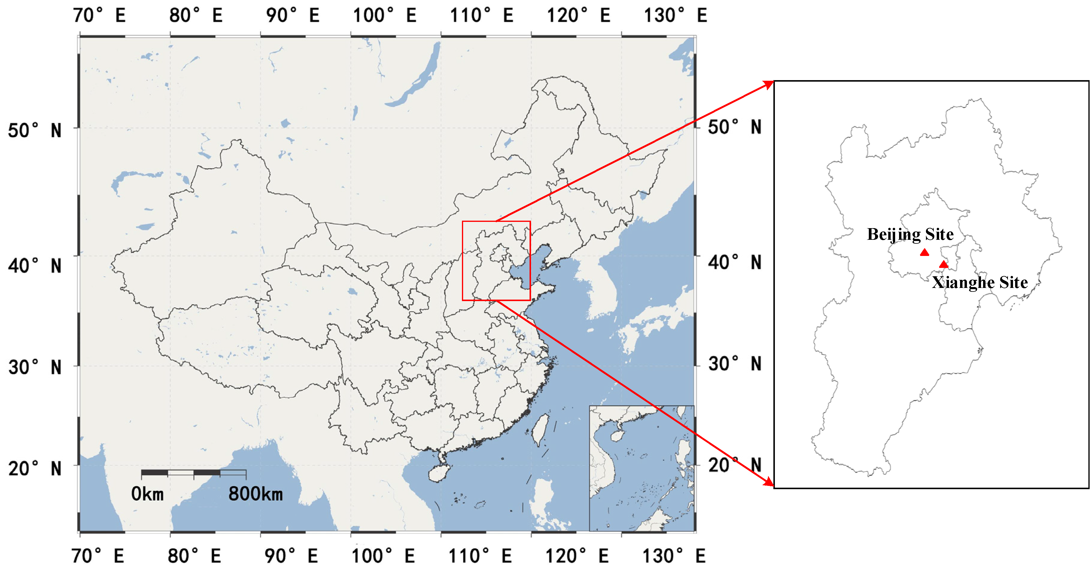
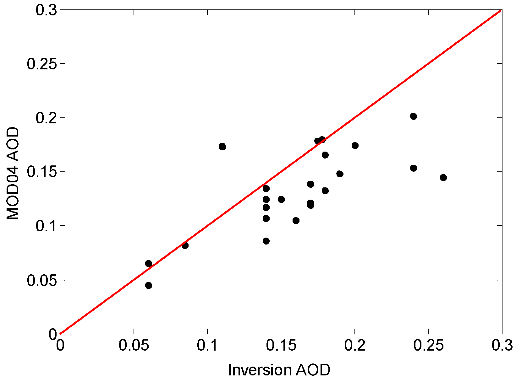
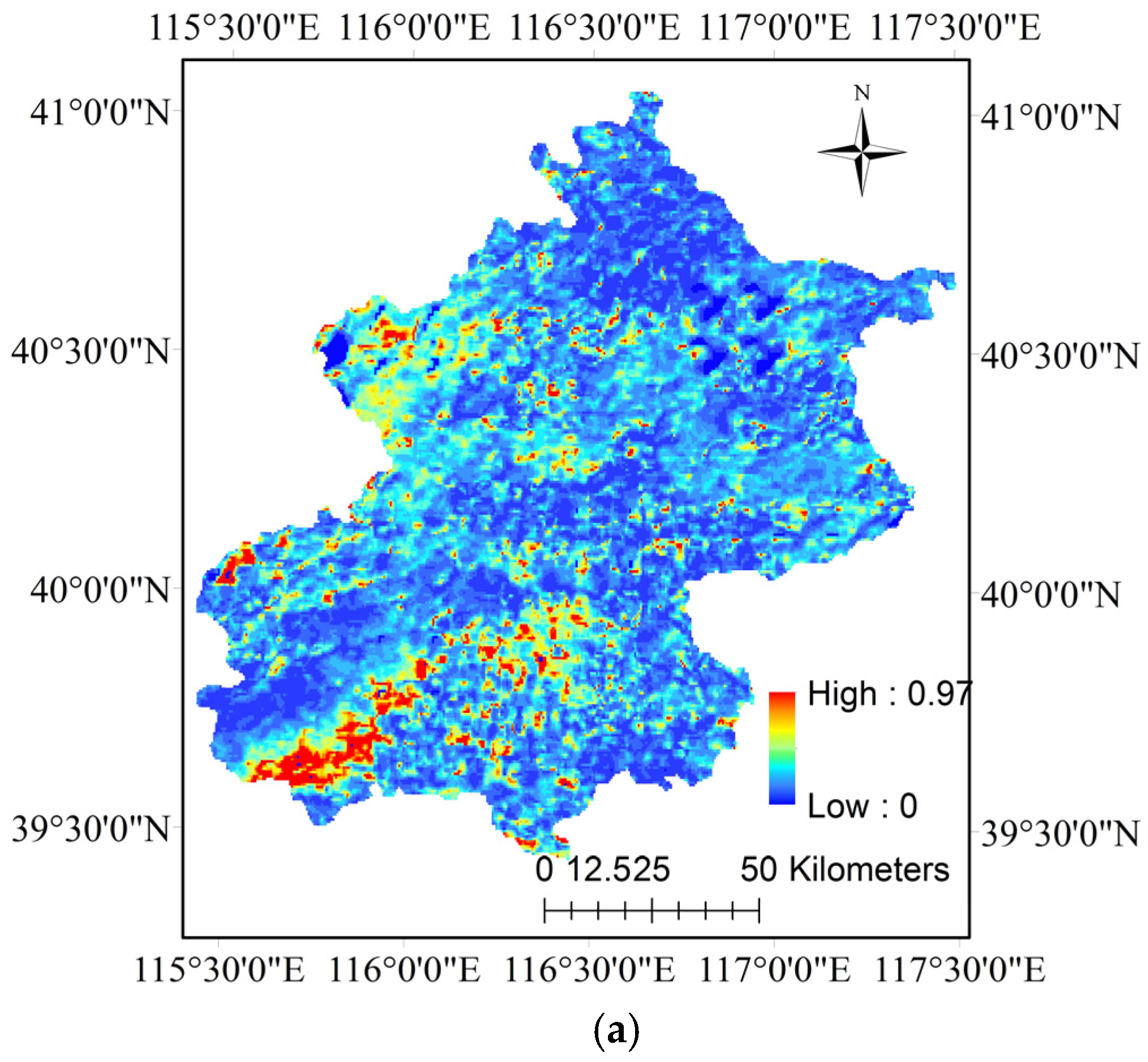
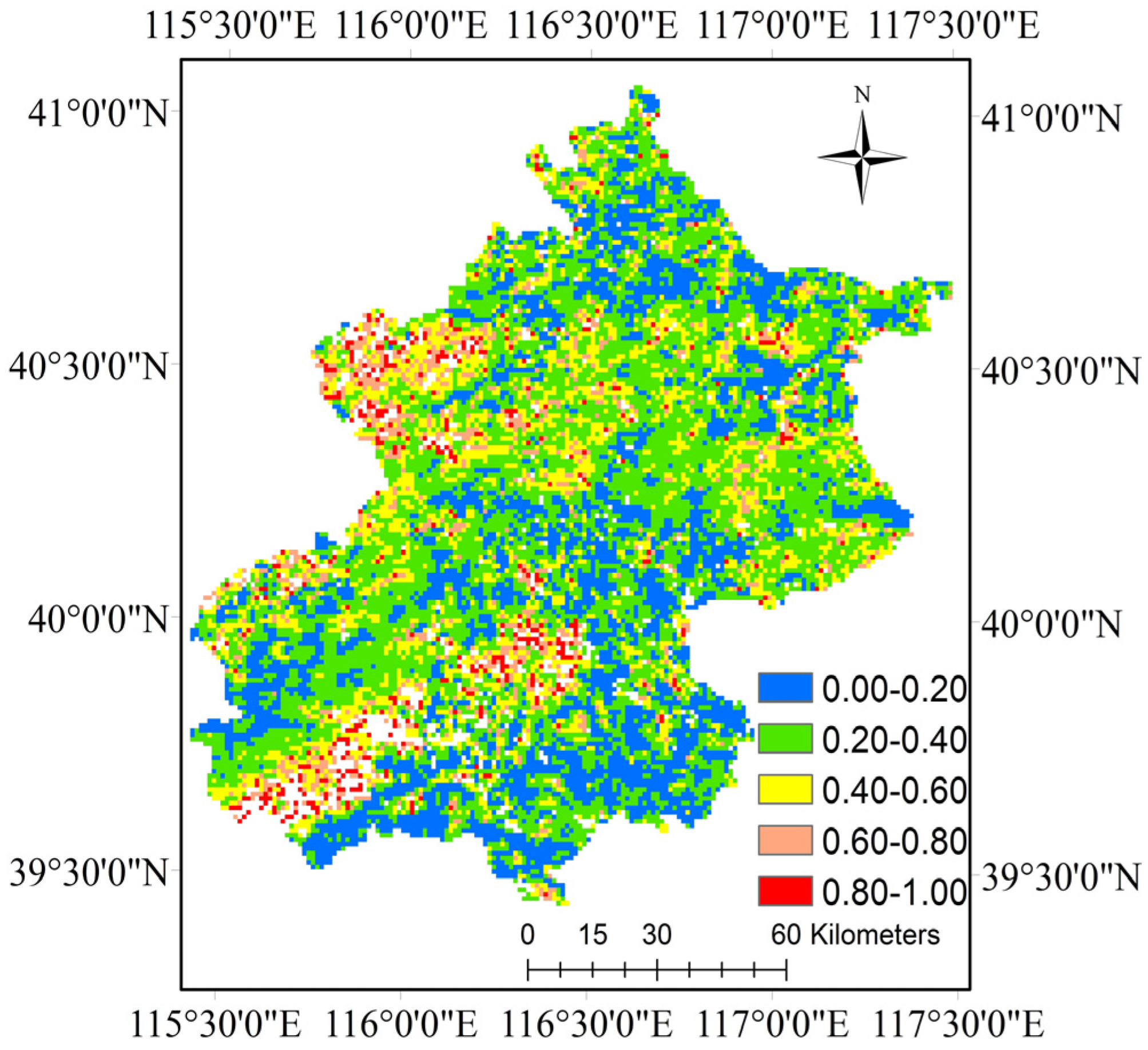
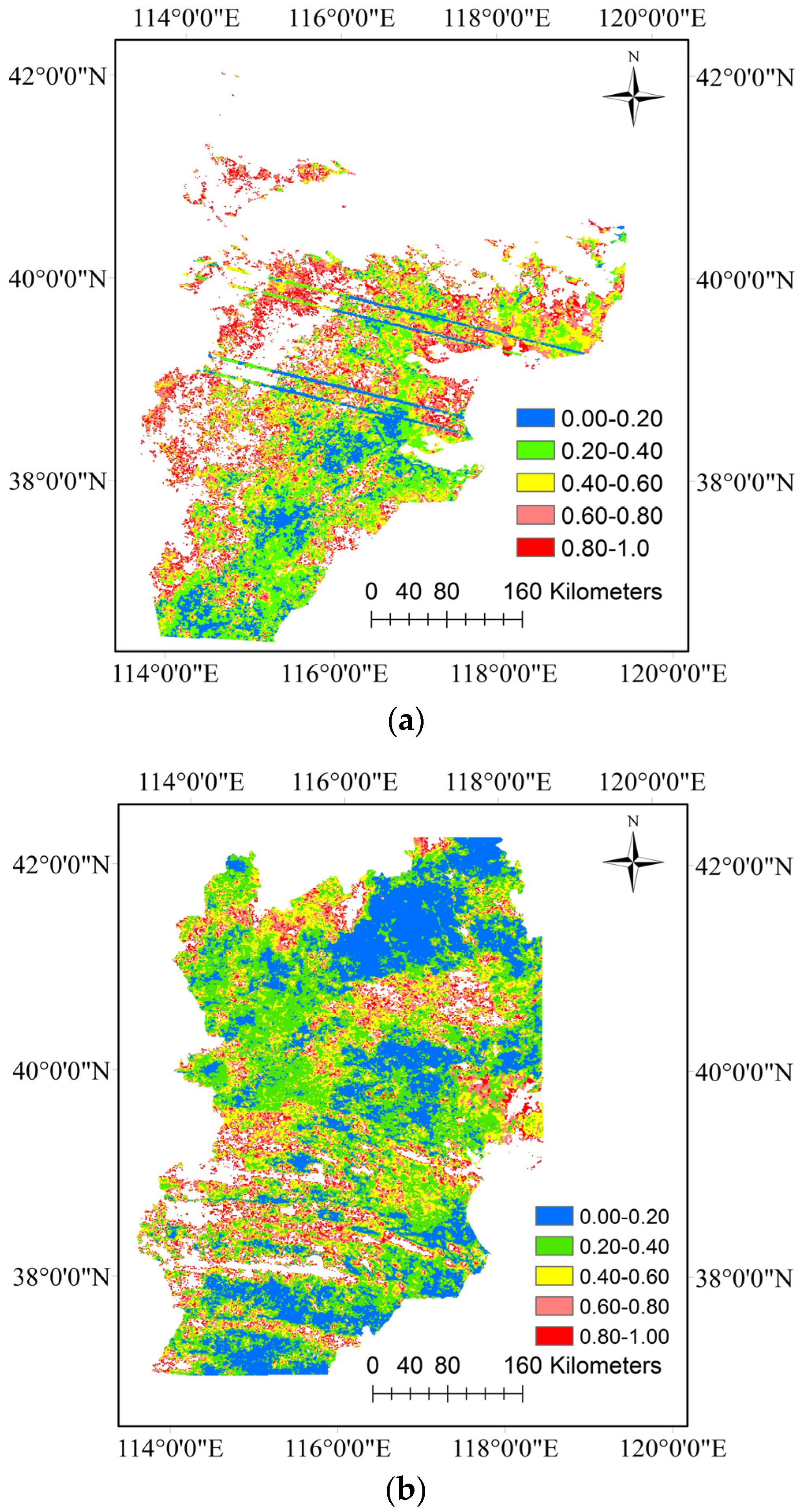
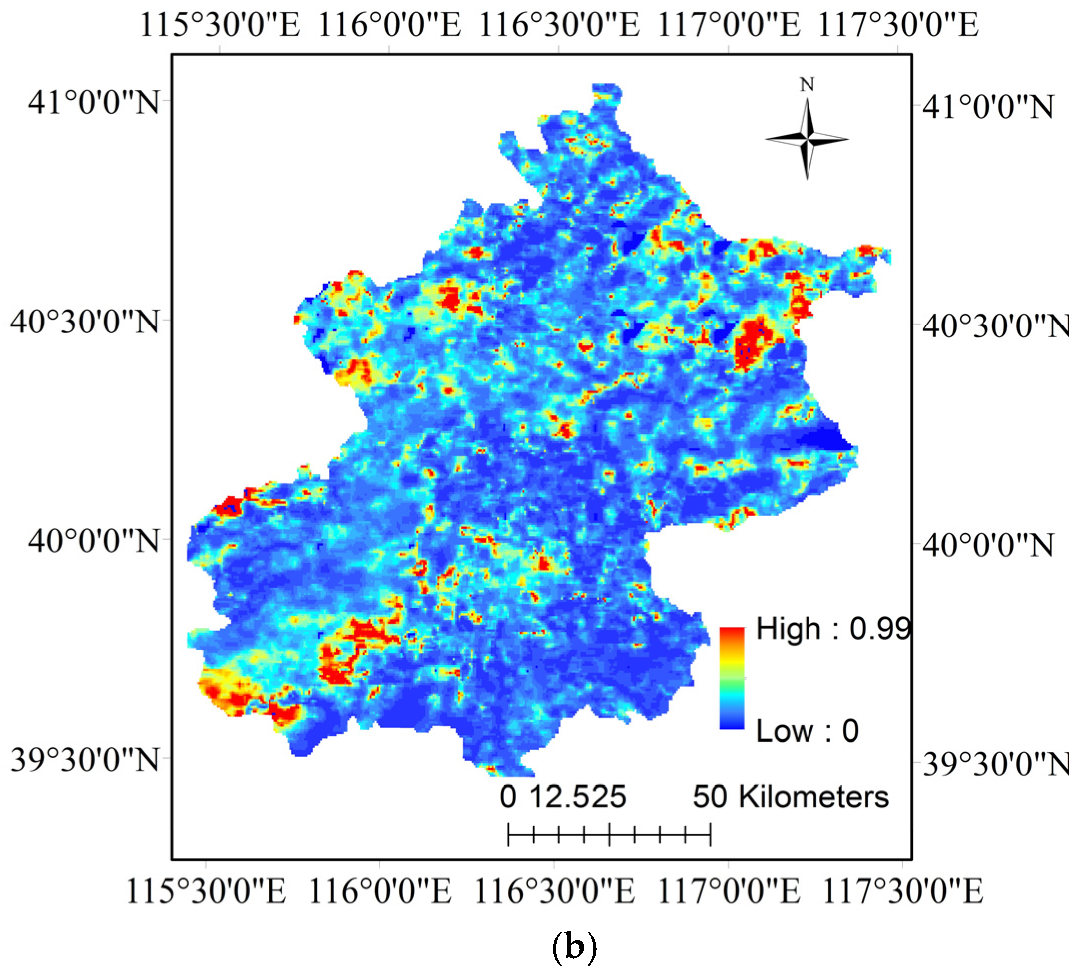
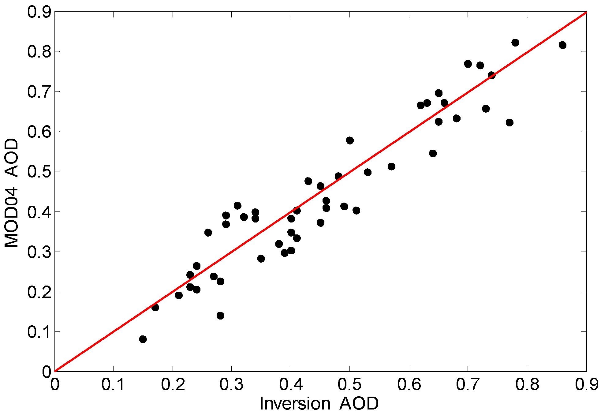
This paper utilizes one kilometer resolution MODIS L1B data and three kilometers resolution MOD 04 aerosol products. The acquisition dates of clear images are 8 February 2015, 10 February 2015 and 5 January 2016. Acquisition dates of inversion images and MOD 04 product are 10 February 2015, 14 February 2015, 7, 12 and 25 January 2016, as were the AERONET observations. The study region is shown in Figure 1. Aerosol optical thickness was retrieved in both Beijing and Beijing–Tianjin–Hebei regions. The study areas were chosen based two considerations. First, in winter, the vegetation coverage of the Beijing–Tianjin–Hebei regions is low, so the surface renders high reflectance characteristics. Second, Beijing and Xianghe site observations could be obtained to verify the accuracy of inversion and MOD 04 AOD.

2.2. Method

Tanre et al. [11] defined and used a structure function to derive the aerosol optical thickness over land surface from satellite data. By assuming the ground reflectance was invariant during a certain period, variations of satellite signal may be attributed to variations of the atmospheric optical properties. It is also assumed that the atmosphere was horizontally uniform and the surface was Lambertian. As mentioned by Tanré [11], the apparent reflectance, ρ * , observed by the satellite could be written as
ρ * ( μ s , μ v , φ ) = ρ a ( μ s , μ v , φ ) + T ( μ s ) [ ρ × e τ / μ v + < ρ > t d ( μ v ) ] 1 < ρ > s
where μ s = cos θ s and θ s is the solar zenith angle, μ v = cos θ v and θ v is the satellite zenith angle, φ is the relative azimuth angle between solar and satellite, ρ a is atmospheric reflectance, T is the total transmittance on the sun-ground path, ρ is the ground surface reflectance, τ is the atmospheric optical depth, < ρ > is the mean surface reflectance, td is the diffuse transmission function on the ground-satellite path, and s is the atmospheric albedo.
We assume the multiple reflective interactions between the surface and the atmosphere are small and thus can be ignored in clear weather. That means the < ρ > s term approach to zero. Furthermore, let us assume the environmental contribution of the surroundings is equivalent, i.e., the < ρ > values are the same in a small local area.
Consequently, the apparent reflectance difference, Δ ρ ( i , j ) * ( d ) , of two adjacent pixels in spatial dimension, ( i , j ) and ( i , j + d ) , with distance d can be derived from Equation (1):
Δ ρ ( i , j ) * ( d ) = ρ ( i , j ) * ρ ( i , j + d ) * = Δ ρ ( i , j ) T ( μ s ) e τ / μ s
where i and j are the row and column indices of the image, respectively. If the surface property does not change in the observation period, i.e., Δ ρ ( i , j ) ( d ) is constant, the difference of the apparent reflectance may be a function of the optical depth. Then, the relationship Δ ρ * 2 and Δ ρ 2 can be expressed as
Δ ρ * 2 = Δ ρ 2 [ T ( μ s ) e τ / μ s ] 2
We can replace T ( μ s ) e τ / μ s by T ( μ s , μ v , τ ) , then, we get
Δ ρ * 2 ( t 1 ) = Δ ρ 2 ( t 1 ) T 2 ( μ s ( t 1 ) , μ v ( t 1 ) , τ ( t 1 ) )
and
Δ ρ * 2 ( t 2 ) = Δ ρ 2 ( t 2 ) T 2 ( μ s ( t 2 ) , μ v ( t 2 ) , τ ( t 2 ) )
where t 1 and t 2 represent two different dates. t 1 is so close to t 2 that it was assumed that the surface reflection characteristics of these two days did not change. In other words, Δ ρ 2 ( t 2 ) can be replaced by Δ ρ 2 ( t 1 ) . We assumed that the day t 1 was a clear day, and the aerosol characteristics did not vary from t 1 to t 2 . Then, we can get
Δ ρ * 2 ( d , t 2 ) Δ ρ 2 ( d , t 1 ) × T 2 ( μ s ( t 2 ) , μ v ( t 2 ) , τ ( t 2 ) ) T 2 ( μ s ( t 1 ) , μ v ( t 1 ) , τ ( t 1 ) )
From Equation (8), we know when d is large (rather than a few pixels), then ρ i , j + d is no longer correlated to ρ i , j ; M * 2 ( ) and M 2 ( ) reduce to the standard deviations, ρ * 2 and ρ 2 . Let M * 2 ( d , t 2 ) and M * 2 ( d , t 1 ) stand for the apparent structure functions of some scene from satellite images at two various dates t 1 and t 2 . In addition we replaced Δ ρ * 2 ( d , t 2 ) and Δ ρ 2 ( d , t 1 ) with M * 2 ( d , t 2 ) and M 2 ( d , t 1 ) . Then, the structure function method can be expressed by
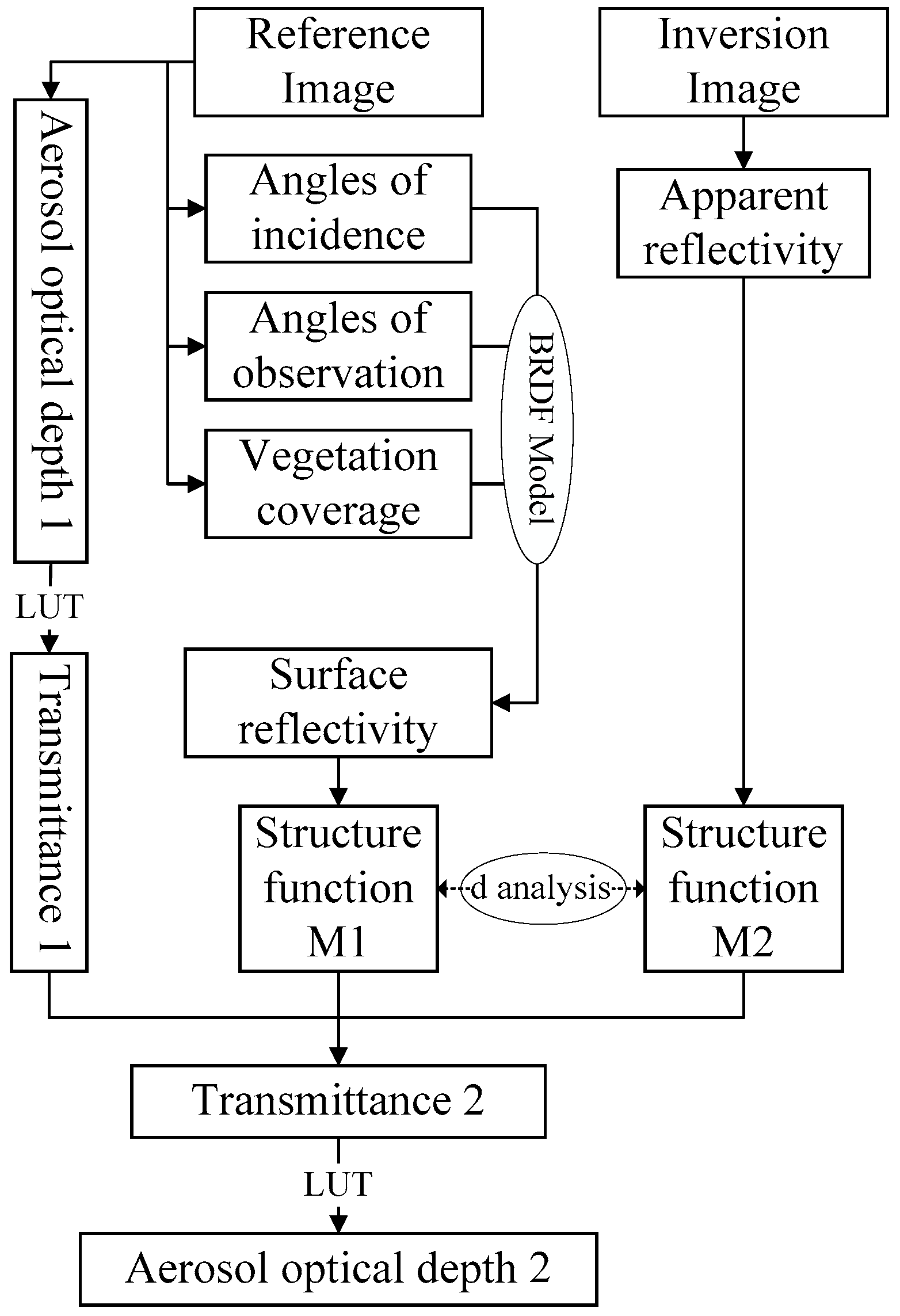
M * 2 ( d , t 2 ) = M 2 ( d , t 1 ) × T 2 ( μ s ( t 2 ) , μ v ( t 2 ) , τ ( t 2 ) ) T 2 ( μ s ( t 1 ) , μ v ( t 1 ) , τ ( t 1 ) )
where T denotes atmosphere total transmittance which is determined by solar zenith angle, sensor zenith angle and aerosol optical depth
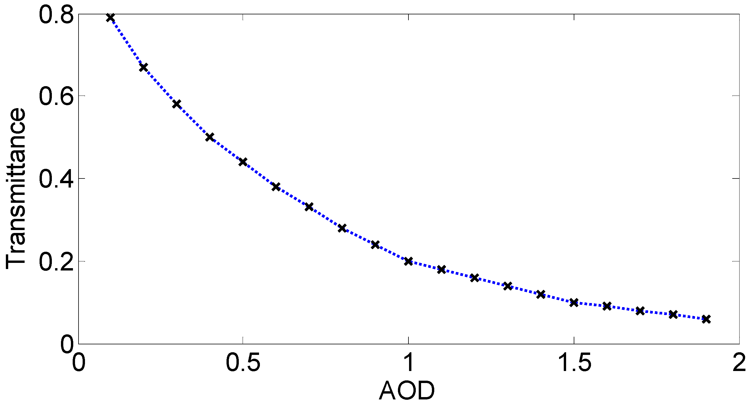
 τ . As shown in Figure 2, the atmosphere transmittance has a negative relationship to the AOD. This connection can be simulated in Second Simulation of the Satellite Signal in the Solar Spectrum (6S) model. If the aerosol optical thickness τ ( t 1 ) is given, then we can calculate T1 via a look-up table (LUT) about Transmittance and AOD. The structure function value M * 2 ( d , t 2 ) and M * 2 ( d , t 1 ) can be calculated with Equation (3). When we get the ratio of M * 2 ( d , t 2 ) to M * 2 ( d , t 1 ) (which is also the ratio of T2 to T1), the transmittance T2 can be obtained. Finally, we calculated AOD τ ( t 2 ) via the same lookup table regarding Transmittance and AOD.
Holben et al. [12] put forward a kind of algorithm to calculate the value of structure function:
M 2 ( d ) = 1 n ( m d ) i = 1 n j = 1 m d ( ρ i , j ρ i , j + d ) 2
where m denotes the number of rows and n the columns. The parameter ρ denotes surface or apparent reflectance. The d value must be set artificially before the calculation. When the d value is changed, the structure function values will also change accordingly, whereby the ratio of two structure function values, and also transmittance ratio, will change. As the structure function values are generally small, a tiny change of structure function value can make big change to the ratio. If the step of Transmittance and AOD in the lookup table is not small enough, the error of calculated AOD value may greatly increase. Therefore, the AOD inversion results will be significantly affected by the d value [11,17].
One of the main theories used in geostatics is the variogram, which is used as a theoretical function. It is the actual realization of the random process Z ( x ) on the ground [29,30]. As the variogram is also known as a ‘structure function’, the algorithm of structure function (Equation (8)) is similar to that of the variogram (Equation (11)), so we applied the geostatistics method to determine the d value.
In a particular direction, along the one-dimensional x-axis, for example, the semivariogram γ ( x , h ) can be described as
γ ( x , h ) = 1 / 2 V a r [ Z ( x ) Z ( x + h ) ] = 1 / 2 E [ Z ( x ) Z ( x + h ) ] 2 1 / 2 { E [ Z ( x ) ] E [ Z ( x + h ) ] } 2
where h is the separation between samples in both distance and direction; Z ( x ) and Z ( x + h ) are the values of Z at places x and x + h; E denotes the expectation, and Var denotes the covariance; 1/2 is just for convenience without practical significance, so we generally call γ ( x , h ) the variogram.
Variables, such as air temperatures, rainfall, the heights of underground water level, and the concentrations of elements in soil, for example, are regarded as spatial random effects. However, for each of these variables, we have only one single realization. We cannot compute statistics or draw inferences from it because inference requires many realizations. In addition, to overcome this impasse, we must make a further assumption that the process is stationary or meets the intrinsic hypothesis [31]. That means for any h, E [ Z ( x + h ) ] = E [ Z ( x ) ] , so γ ( x , h ) can be given by
γ ( x , h ) = 1 / 2 E [ Z ( x ) Z ( x + h ) ] 2
where γ ( x , h ) depends only on the distance h and is not relevant with the position of x, it can be recorded as γ ( h ) . We can get close to the regional variogram with dense data from satellite and proximal sensors when we compute their experimental variograms. It is usually computed by the method of moments and attributed to Matheron [32]:
γ * ( h ) 1 2 N ( h ) i = 1 N ( h ) [ Z ( x i ) Z ( x i + h ) ] 2
where N(h) is the number of paired comparisons at lag h.
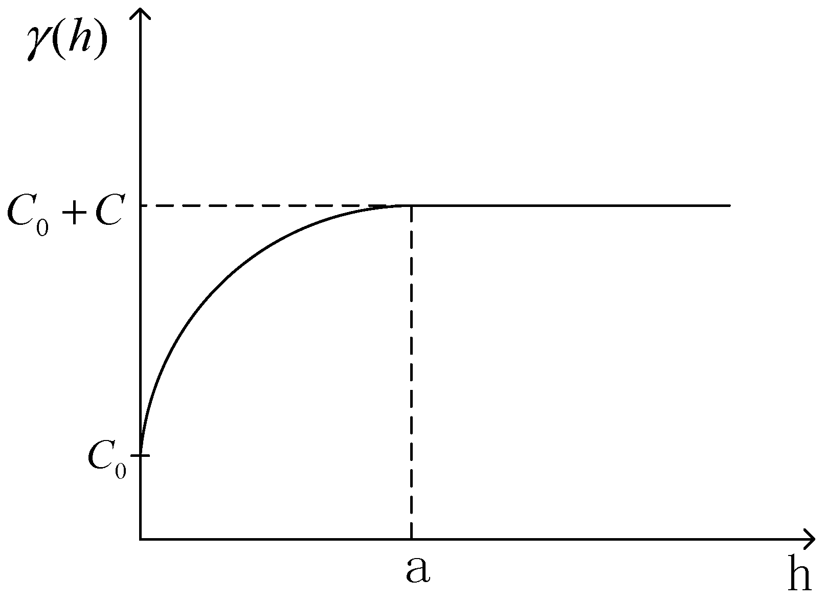
Generally, variogram γ ( h ) is monotone increasing, but no longer when h > a (range a > 0) instead of being stable near a limit value. This suggests that all directional variograms have good spatial structures in their range. The ideal variogram curve is shown in Figure 3. When | h | 0 , γ ( h ) C 0 , meaning nugget effect, and C 0 (> 0) is called nugget constant; when | h | + , γ ( h ) C 0 + C = C ( 0 ) and C 0 + C is called the sill value, and is equal to the priori covariance C ( 0 ) .
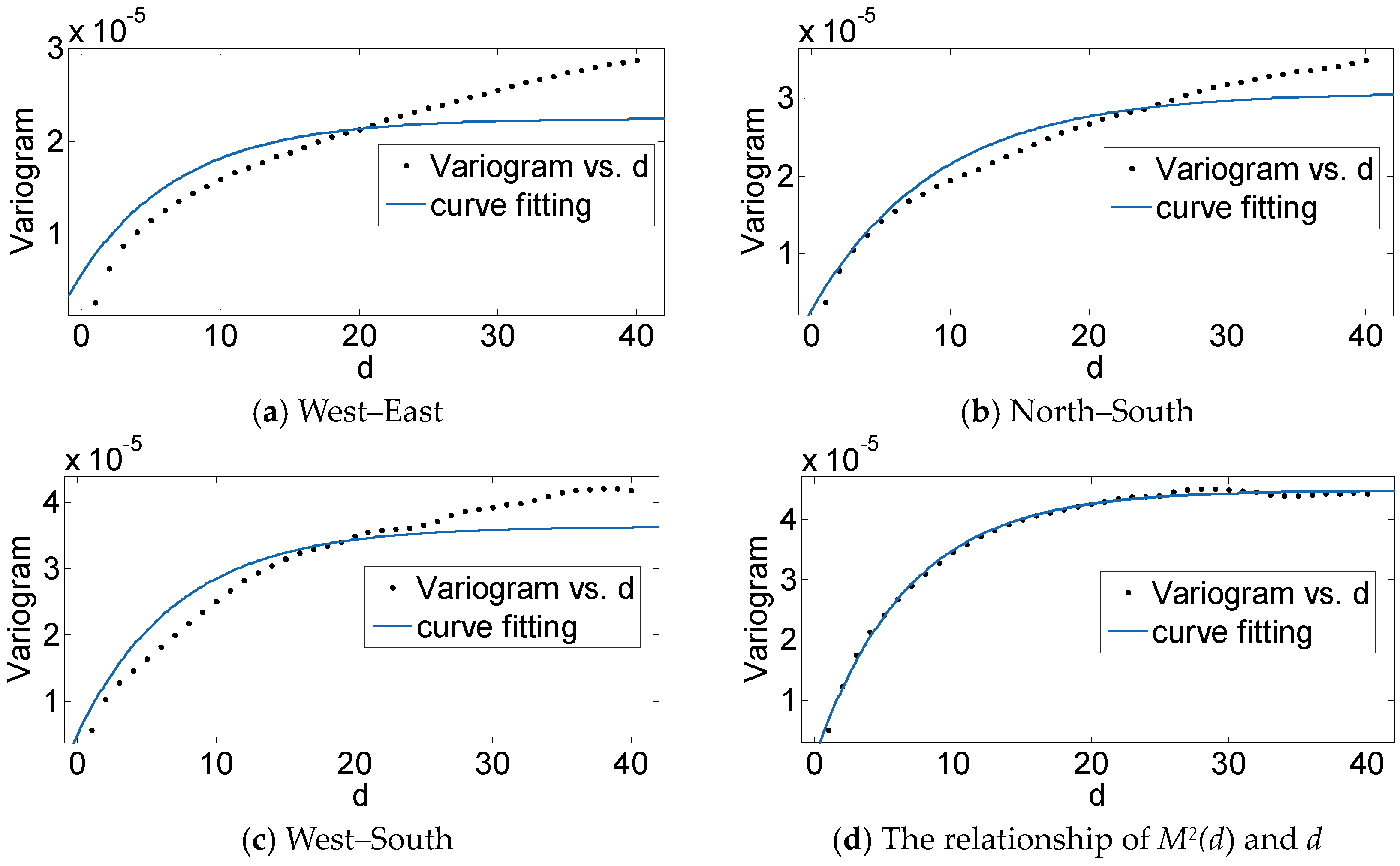
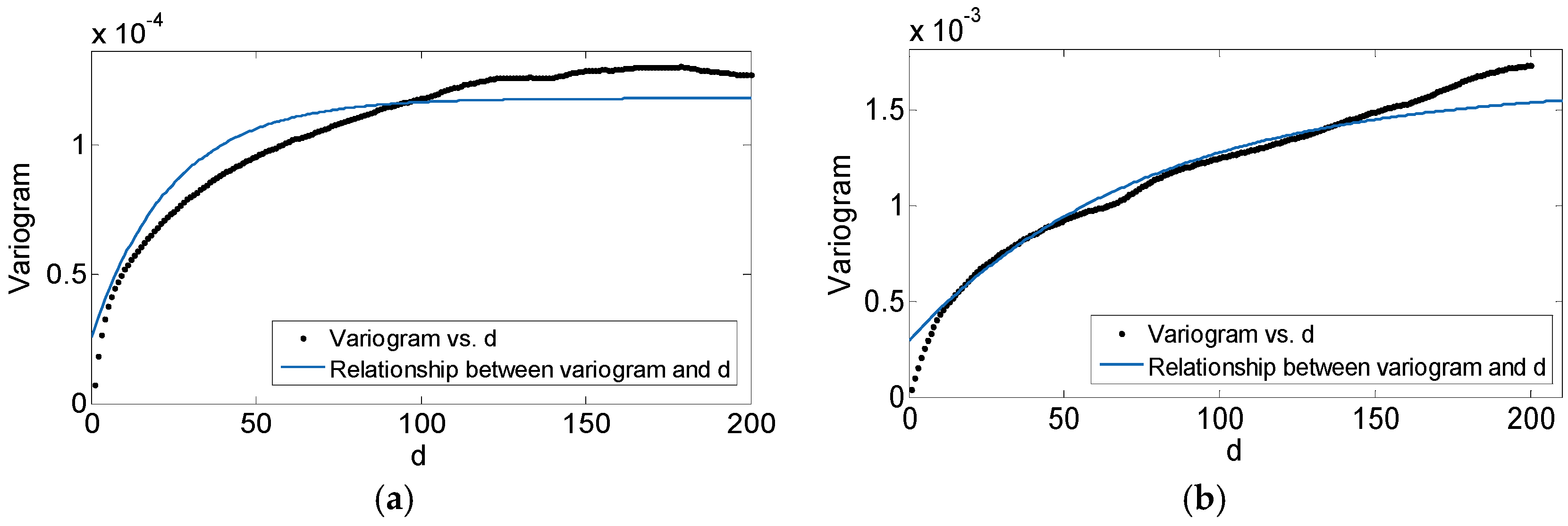
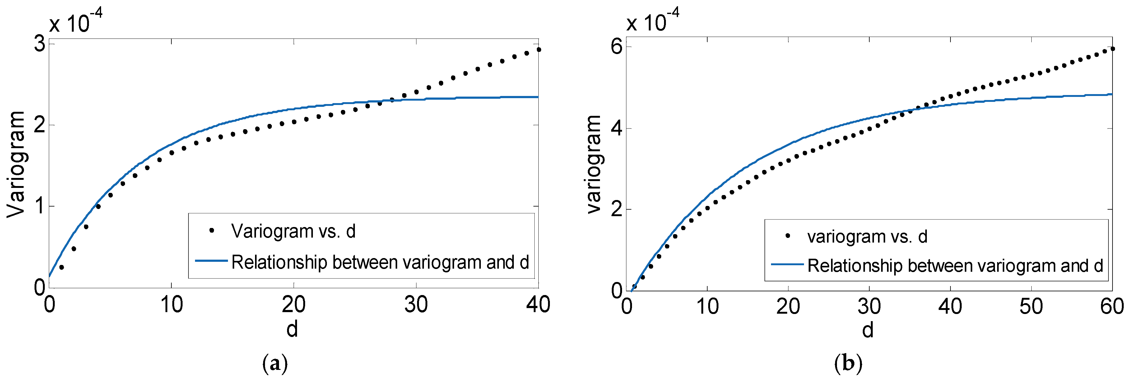
Range a is actually the spatial variation scale (also called spatial autocorrelation scale) of regionalized variables. When we apply variogram theory to structure function, h can be replaced by d and γ ( h ) replaced by M 2 ( d ) . If we set d at a value not less than a, the variables ground or apparent reflectance ρ i , j does not have spatial correlation with ρ i , j + d . In other words, the value of M 2 ( d ) can be considered not to change with d values. Thus, we think the M 2 ( d ) is stable enough. In the process of actual calculation, we find that M 2 ( d ) has a good fitting effect with the variogram exponential model. Thus, we can use the exponential model to analyze the range of structure function.

3. Results and Discussion

3.1. Variogram and d

We selected one MODIS image of the Beijing region (178 km × 180 km, 1 kilometer resolution), acquired on 7 January 2016, for our research samples. Here, we supposed that regional variable surface reflectance met second-order stationary hypothesis or intrinsic hypothesis, which allowed for the calculation of experimental variogram values. By incrementing d of west-east, north-south and west-south direction in step one, we obtained an ordered set of values, as shown by the points plotted in each of the graphs in Figure 4. Furthermore, we used the exponential model to fit these points, and the fitting curves are also shown in Figure 4.
One kind of structure function algorithm is given by Liu et al. [14]:
M 2 ( d ) = 1 3 ( m d ) ( n d ) i = 1 n d j = 1 m d [ ( ρ i , j ρ i , j + d ) 2 + ( ρ i , j ρ i + d , j ) 2 + ( ρ i , j ρ i + d , j + d ) 2 ]
where m denotes the number of rows and n the columns. ρ denotes surface reflectance. M 2 ( d ) can be regarded as the registration of the variogram in three directions. In the same way, we analyzed the exponential fitting curve of M 2 ( d ) for d, as shown in Figure 4d. All of the results are described in more detail in Table 1.
For the exponential model:
γ ( h ) = { 0 h = 0 C 0 + C ( 1 e h / a ) h > 0
when h = 3a, γ ( h ) C 0 + C , this means that the range of the exponential model is 3a. The calculated four range values are also listed in Table 1.
These demonstrate M 2 ( d ) and other three directional variograms have a similar change rule. Additionally, the correlation coefficients fitting with the exponential model are all above 0.9. In particular, M 2 ( d ) has the highest correlation. In order to ensure that M 2 ( d ) has a certain stability, d should not be less than the range. As a consequence, d can be set to 20 for the selected MODIS image in this paper.

3.2. AOD Inversion Results and Discussion

As shown in Figure 5, a clear image was first selected from a series of MODIS data which was acquired on 5 January 2016. The clear image was used to provide information on surface vegetation and observation angles for the Meister’s Bidirectional Reflectance Distribution Function (BRDF) model [33]. Then, the structure function M1 was calculated using the BRF map. For the bright surface, the surface reflectance relationship between infrared and red or blue wave band is not stable enough, thus, we cannot calculate the surface reflectance by using empirical formula. However, we can calculate the surface reflectance using the BRDF model through the relationship between the BRF and other parameters and means that we improved the traditional structure function method for aerosol retrieval coupled with the BRDF model. Subsequently, a second image (acquired on 7 January 2016) was selected to calculate the structure function M2. During the process of calculating the structure function M1 and M2, the selection of the value of pixel space d proved to be of great importance. In order to solve this problem, variogram theory was referenced. We analyzed the relationship between variogram and d to determine the d value. Following this process, we retrieved the aerosol optical thickness using a look-up table, which was calculated using the 6S model.
Finally, we obtained an AOD distribution map, as shown in Figure 6. With the exception of the areas covered by cloud—such as the north-west region—the AOD results have many effective pixels.
The inversion result was then compared with the MODIS aerosol product (MOD 04 product), and the error was analyzed. We chose 25 sets of data from the inversion result and the MOD 04 product at random according to the geographical coordinates, and calculated the absolute and relative errors. The greatest absolute error was 0.115; however, the greatest relative error is more than 80%, possibly due to the pixel deviation between the retrieval result and the MOD 04 product result or the negligence of the water vapor content of the aerosol. Table 2 and Figure 7 show the statistics of the AOD values. For all 25 sets of samples, the average absolute error (unsigned numbers) is 0.039, and the relative error is 29.69%.
Since the uncertainties existed in the retrieval algorithms, sensor degradation problems and other aspects, various MODIS AOD products need to be evaluated in different seasons and regions in order to enhance their accuracy for diverse application [34,35]. A comparison was also made between inversion AOD and MOD 04 AOD with AERONET AOD data. The MODIS image was acquired at 02:55 (UTM) on 7 January 2016, so we chose AERONET Beijing site (39°58′37″ N, 116°22′51″ E) data from the time period 02:28 to 03:21. Not all AERONET sites have observations at 660 nm (nanometer), so the consistency of the validation data was taken into account. To obtain an AOD from the 660 nm band, we needed to make an AOD interpolation from two bands of 440 nm and 870 nm. Detailed data and processing results are shown in Table 3.
We selected the pixel points in the inversion AOD image which corresponded to the location of the AERONET Beijing site. To avoid the influence of cloud pixels, we selected one point at four pixels apart (less than 5 km) from the corresponding point. The average AOD of the selected point and the surrounding eight points is calculated as the inversion result, and shown in Table 4.
Therefore, the absolute error is −0.00187 and the relative error is 0.99%.
For the MOD 04 product, there was a lot of missing data, including the points near the AERONET Beijing site. Thus, the nearest point in the same direction with the AOD of the corresponding missing point was selected. This resulted in the MOD_04 AOD value of 0.180, the absolute error of −0.00854, and the relative error of 4.53%. After comparing the two sets of data, we can see that the improved structure function method has a good inversion effect, a higher accuracy and more effective data points.

4. Validation

We applied the new method to the Beijing–Tianjin–Hebei region for aerosol optical thickness inversion to further verify the method we presented. As mentioned in Section 3, the relationship of the variogram and d is analyzed, as shown in Figure 8, with the fitting details shown in Table 5. We can see that the variogram and d value have a good fitting effect. Therefore, the range of fitting is 93 and 224. Finally we set the d value at 100 and 225, no less than the fitting range.
Finally, the aerosol optical thickness inversion spatial distribution of the Beijing–Tianjin–Hebei region was obtained and is shown in Figure 9. There are still a lot of effective data even though many pixels are missing due to cloud. In Figure 9a, the image has four obvious “dividing lines” because the image used for inversion is from two merged original MODIS images. Among the stitching image, two or three rows of data are nonexistent and seen as the first dividing line. After a process of structure function value calculation, there are two further dividing lines. During the comparison of two structure function values, four dividing lines are formed.
For validation of a different resolution, we applied the new method to MODIS 500 m resolution images. As mentioned in Section 3, the relationship of the variogram and d is analyzed, and shown in Figure 10 with the fitting details shown in Table 6. Therefore, the ranges of fitting are 23 and 44. Finally the d value was set at 25 and 45, no less than the range of fitting. Finally, the aerosol optical thickness inversion spatial distribution of the Beijing region was obtained and is shown in Figure 11.
For further validation of the inversion effect, we compared inversion AOD and MOD 04 AOD where a total of 50 contrast points were obtained. Figure 12 and Table 7 show the statistics of the AOD values retrieved from the MODIS image compared to the MOD 04 AOD. The validation results show that inversion AOD exhibits high consistency with MOD 04 AOD. For all sample points, the average absolute error (unsigned numbers) is 0.055, and the relative error is 16.28%.
In order to compare the accuracy of both MOD 04 AOD and inversion AOD, we continued to use AERONET observations. There are four AERONET data sites in the Beijing–Tianjin–Hebei region: Beijing, the Institute of Remote Sensing and Digital Earth Chinese Academy of Sciences (RADI) in Beijing, the Chinese Academy of Meteorological Sciences (CAMS) in Beijing, and Xianghe; however, there are no AOD values in the MOD 04 product for three of the observation sites on 10 February 2015. As a result, only the Beijing site (39°45′14″ N, 116°57′43″ E) was chosen to calculate the errors as shown in Table 8. For the MOD 04 AOD, the absolute error is −0.0514 and the relative error is 17.16%. Obviously, the inversion AOD has a higher accuracy with the absolute error of 0.0056 and the relative error of 1.88%. For data acquired on 14 February 2015, only the errors of inversion AOD were calculated. For 500 m resolution validation, inversion AOD also has a smaller relative error (2.87% instead of 50.93%) and absolute error (−0.00192 instead of 0.03408) for 12 January 2016. For 25 January 2016, the relative error and the absolute error of inversion AOD are both smaller than MOD 04 AOD, with 0.00492 to −0.03686 and 5.30% to 39.69%.

5. Conclusions

We have improved an aerosol optical depth reversion algorithm by introducing variogram theory to discuss how to set the d value in the calculation process of structure function. We applied the new method to a MODIS L1B image of the Beijing region. The inversion results were verified by using the MODIS AOD product and the AERONET AOD data. In this paper, we applied the new method to more study regions for validation.
The methodology of d determined is based on range inference. Relations between structure function values and d values are fitted by the variogram exponential model. When the range is calculated using the empirical formula, we can set the d value at no less than the range.
For the MODIS image acquired on 7 January 2016, in the Beijing region, the resolution was one kilometer and the range was calculated as 20, therefore, the d value was set at 20. Subsequently, AOD inversion results were obtained using structure function. Compared with MOD 04 AOD, the statistical results of 25 sets of co-location samples shows that the average absolute error is 0.039 and the relative error is 29.69%. Furthermore, we verified both the inversion and MOD 04 AOD results by using the AERONET Beijing site AOD data. The inversion AOD has a smaller relative error (0.99% instead of 4.35%) and an absolute error (−0.00187 instead of −0.00854).
For regional validation, we applied this new method to the Beijing–Tianjin–Hebei region. For the MODIS image acquired on 10 February 2015, the range is calculated as 93 and thus d set to 100. For the MODIS image acquired on 14 February 2015, the range is 224 and d set to 225. Inversion AOD also has a higher accuracy for 10 February 2015 based on AERONET observations. Unfortunately, a conclusion cannot be reached for 10 February 2015, as the MOD 04 did not have any co-location data. Furthermore, inversion AOD has a higher resolution (one kilometer instead of three kilometers) and more effective pixels.
For resolution validation, we applied this method to MODIS 500 m resolution images. The value of d is set to 25 and 45 for 12 and 25 January 2016, respectively. The results show that inversion AOD also has a higher accuracy.
We feel it is important to point out that the structure function has one big limitation: this method is not suitable if there is a lot of cloud in the satellite images. As a result, it is one of the reasons as to why it can be difficult to find suitable inversion images and reference images.

Acknowledgments

This work was jointly supported by the National Key Research and Development Program of China (Grant No. 92016YFC0201800), Research on Data Processing Theory and Methods of the Auxiliary Lines Selection Based on Satellite Remote Sensing Image (Grant No. GCB17201600036), the Beijing Natural Science Foundation (Grant No. 8162028) , National Natural Science Foundation of China (Grant No. 40901168), Key Laboratory of Space Ocean Remote Sensing and Application Foundation (Grant No. 201602021) and State Key Laboratory of Remote Sensing Science Foundation, Jointly Sponsored by the Institute of Remote Sensing and Digital Earth of Chinese Academy of Sciences and Beijing Normal University (Grant No. OFSLRSS201506). The authors thank NASA for providing the MODIS data and maintaining the AERONET sites used in this study. The authors are also grateful to the anonymous reviews for their valuable comments.

Author Contributions

Guanhua Zhou and Yue Zhang conceived the study and wrote the manuscript. Zhongqi Ma and Wujian Xu participated in the experiments and data analysis. Kai Zhang, Junhui Liu and Yumin Tan contributed to the discussion of the results.

Conflicts of Interest

The authors declare no conflict of interest.

References

  1. Carslaw, K.S.; Bouvher, O.; Spracklen, D.V.; Mann, G.W.; Rae, J.G.L.; Woodward, S.; Kulmala, M. A review of natural aerosol interactions and feedbacks within the Earth system. Atmos. Chem. Phys. Dicuss. 2009, 9, 11087–11183. [Google Scholar] [CrossRef]
  2. King, M.D.; Kaufman, Y.J.; Tanré, D.; Nakajima, T. Remote sensing of tropospheric aerosols from space: Past, present and future. Bull. Am. Meteorol. Soc. 1999, 80, 2229–2260. [Google Scholar] [CrossRef]
  3. Reisen, F.; Meyer, C.P.; Keywood, M.D. Impact of biomass burning sources on seasonal aerosol air quality. Atmos. Environ. 2013, 67, 437–447. [Google Scholar] [CrossRef]
  4. Pope, C.A.; Dockery, D.W. Health effects of fine particulate air pollution: Lines that connect. J. Air Waste Manag. Assoc. 2006, 56, 709–742. [Google Scholar] [CrossRef] [PubMed]
  5. Hayood, J.M.; Boucher, O. Estimates of the direct and indirect radiative forcing due to tropospheric aerosols: A review. Rev. Geophys. 2000, 38, 513–543. [Google Scholar] [CrossRef]
  6. Lohmann, U.; Feichter, J.G. Indirect aerosol effect: A review. Atmos. Chem. Phys. 2005, 5, 715–737. [Google Scholar] [CrossRef]
  7. Kokhanovsky, A.A.; Leeuw, G. Satellite Aerosol Rmote Sensing Over Land; Springer: Berlin/Heidelberg, Germany; New York, NY, USA, 2009. [Google Scholar]
  8. Tian, X.P.; Sun, L. Retrieval of aerosol optical depth over arid areas from MODIS data. Atmosphere 2016, 7, 134. [Google Scholar] [CrossRef]
  9. Sun, L. Remote Sensing of Aerosols over Urban Areas. Ph.D. Thesis, Institute of Remote Sensing Applications Chinese Academy of Science, Beijing, China, 2006. [Google Scholar]
  10. Huang, T. Three Methods of Aerosol Optical Thickness Inversion in Lanzhou Using MODIS Data. Master’s Thesis, Lanzhou University, Lanzhou, China, 2005. [Google Scholar]
  11. Tanre, D.; Deschamps, P.Y.; Devaux, C.; Herman, M. Estimation of saharan aerosol optical thickness from blurring effects in thematic mapper data. J. Geophys. Res. 1988, 93, 15955–15964. [Google Scholar] [CrossRef]
  12. Holben, B.; Vermote, E.; Kaufman, Y.J.; Tanré, D.; Kalb, V. Aerosol retrieval over land from AVHRR data-application for atmospheric correction. IEEE Trans. Geosci. Remote 1992, 30, 212–222. [Google Scholar] [CrossRef]
  13. Lin, T.H.; Liu, Z.R.; Chen, Z.J. Method of aerosol optical thickness inversion by using SPOT data. J. Photogramm. Remote Sens. 1998, 3, 1–14. [Google Scholar]
  14. Liu, G.R.; Chen, A.J.; Lin, T.H.; Kuo, T.H. Applying SPOT data to estimate the aerosol optical depth and air quality. Environ. Model. Softw. 2002, 1, 3–9. [Google Scholar] [CrossRef]
  15. Sun, L. The Study of Remote Sensing Inversion of Atmospheric Aerosol over Urban Areas. Ph.D. Thesis, the Graduate School of Chinese Academy of Sciences, Beijing, China, 2006. [Google Scholar]
  16. Xu, F.F. Aerosol Optical Thickness Inversion Using Structure Function Method Supported By the Surface Reflectivity Products. Master’s Thesis, Shandong University of Science and Technology, Qingdao, China, 2012. [Google Scholar]
  17. Zhu, L.; Sun, L.; Yang, L.; Xu, F.F.; Xu, Q.S. Pixel distance settings in aerosol optical depth retrieval through the structure function method. J. Remote Sens. 2016, 4, 528–539. (In Chinese) [Google Scholar]
  18. Wang, L.L.; Wang, Y.S.; Xin, J.Y.; Li, Z.Q.; Wang, X.Y. Assessment and comparison of three years of Terra and Aqua MODIS Aerosol Optical Depth Retrieval (C005) in Chinese terrestrial regions. Atmos. Res. 2010, 97, 229–240. [Google Scholar] [CrossRef]
  19. Remer, L.A.; Kleidman, R.G.; Levy, R.C.; Kaufman, Y.J.; Tanré, D.; Mattoo, S. Global aerosol climatology from the MODIS satellite sensors. J. Geophys. Res. Atmos. 2008, 113, 762–770. [Google Scholar] [CrossRef]
  20. Levy, R.C.; Remer, L.A.; Mattoo, S.; Vermote, E.F.; Kaufman, Y.J. Second-generation operational algorithm: Retrieval of aerosol properties over land from inversion of Moderate Resolution Imaging Spectroradiometer spectral reflectance. J. Geophys. Res. 2007, 112, D13211. [Google Scholar] [CrossRef]
  21. Kaufman, Y.J. Algorithm for remote sensing of tropospheric aerosol from modis. Collect. Prod. ID MOD04/MYD 1998, 80, 2229–2260. [Google Scholar]
  22. Wang, Y.J.; Lyapustin, A.I.; Privette, J.L.; Morisette, J.T.; Holben, B. Atmospheric correction at aeronet locations: A new science and validation data set. IEEE Trans. Geosci. Remote 2009, 47, 2450–2466. [Google Scholar] [CrossRef]
  23. Holben, B.N.; Tanré, D.; Smirnov, A.; Eck, T.F.; Slutsker, I.; Abuhassan, N.; Newcomb, W.W.; Schafer, J.S.; Chatenet, B.; Lavenu, F.; et al. An emerging ground-based aerosol climatology: Aerosol optical depth from AERONET. J. Geophys. Res. 2001, 106, 12067–12097. [Google Scholar] [CrossRef]
  24. Holben, B.N.; Eck, T.F.; Slutsker, I.; Tanre, D.; Buis, J.P.; Setzer, A.; Vermote, E.; Reagan, J.A.; Kaufman, Y.J.; Nakajima, T.; et al. AERONET-a federated instrument network and data archive for aerosol characterization. Remote Sens. Environ. 1998, 66, 1–16. [Google Scholar] [CrossRef]
  25. Chen, H.; Cheng, T.H.; Gu, X.F.; Li, Z.Q.; Wu, Y. Characteristics of aerosols over Beijing and Kanpur derived from the AERONET dataset. Atmos. Pollut. Res. 2016, 7, 162–169. [Google Scholar] [CrossRef]
  26. Pal, S.; Devara, P.A. A wavelet-based spectral analysis of long-term time series of optical properties of aerosols obtained by lidar and radiometer measurements over an urban station in Westen India. J. Atmos. Sol.-Terr. Phys. 2012, 84–85, 75–87. [Google Scholar] [CrossRef]
  27. Eck, T.F.; Holben, B.N.; Reid, J.S.; Dubovik, O.; Smirnov, A.; O Neill, N.T.; Slutsker, I.; Kinne, S. Wavelength dependence of the optical depth of biomass burning, urban, and desert dust aerosols. J. Geophys. Res. 1999, 104, 31333–31349. [Google Scholar] [CrossRef]
  28. Ichoku, C.; Chu, D.A.; Mattoo, S.; Kaufman, Y.J.; Remer, L.A.; Tanre, D.; Slutsker, I.; Holben, B.N. A spatio-temporal approach for global validation and analysis of MODIS aerosol products. Geophys. Res. Lett. 2002, 29. [Google Scholar] [CrossRef]
  29. Oliver, M.A.; Webster, R. A tutorial guide to geostatistics: Computing and modelling variograms and kriging. Catena 2014, 113, 56–69. [Google Scholar] [CrossRef]
  30. Liu, A.L.; Wang, P.F.; Ding, Y.Y. Introduction to Geostatistics; Sciences Press: Beijing, China, 2002. (In Chinese) [Google Scholar]
  31. Cressie, N. When are relative varograms useful in Geostatisties. Math. Geol. 1985, 17, 693–702. [Google Scholar] [CrossRef]
  32. Matheron, G. Principles of geostatistics. Econ. Geol. 1963, 58, 1246–1266. [Google Scholar] [CrossRef]
  33. Meister, G.; Rothkirch, A.; Spitzer, H. Large-Scale bidirectional reflectance model for urban areas. IEEE Trans. Geosci. Remote 2001, 9, 1927–1942. [Google Scholar] [CrossRef]
  34. Levy, R.C.; Remer, L.A.; Kleidman, R.G.; Mattoo, S.; Ichoku, C.; Kahn, R.; Eck, T.F. Global evaluation of the Collection 5 MODIS dark-target aerosol products over land. Atmos. Chem. Phys. 2010, 10, 10399–10420. [Google Scholar] [CrossRef] [Green Version]
  35. Levy, R.C.; Mattoo, S.; Munchak, L.A.; Remer, L.A.; Sayer, A.M.; Patadia, F.; Hsu, N.C. The Collection 6 MODIS aerosol products over land and ocean. Atmos. Meas. Technol. 2013, 6, 2989–3034. [Google Scholar] [CrossRef]
Figure 1. Geographical locations of the study areas as shown on a map of China (left) with the Beijing–Tianjin–Hebei region highlighted on the (right). The two aerosol robotic network sites marked by red triangles are the Beijing and Xianghe Sites.
Atmosphere 08 00006 g001
Figure 2. Relationship of Transmittance and AOD (aerosol optical depth) when solar zenith angle is 30°, sensor zenith angle is 60° and the relative azimuth angle between solar and sensor is 90°.
Atmosphere 08 00006 g002
Figure 3. The ideal variogram curve.
Atmosphere 08 00006 g003
Figure 4. Curve fittings between the variogram and d in four directions: (a) West–East; (b) North–South; (c) West–South; and (d) The relationship of M2(d) and d. The black dots are the actual calculated variogram value and the blue solid lines are the curve fittings. The variogram model is the exponential model.
Atmosphere 08 00006 g004
Figure 5. Flow chart of aerosol optical depth inversion based on structure function.
Atmosphere 08 00006 g005
Figure 6. The aerosol optical depth spatial distribution over Beijing. The inversion image was acquired on 7 January 2016, and the reference image (the clear day) was acquired on 5 January 2016. In this inversion progress, d is set to 20. τ ( t 1 ) is assumed to 0.2.
Atmosphere 08 00006 g006
Figure 7. The AOD comparison of inversion and MOD_04. The black dots represent 25 sets of geographical location, and the red solid line represents y = x.
Atmosphere 08 00006 g007
Figure 8. Relationship between the variogram and d. (a) The acquisition date of the MODIS image is 10 February 2015. (b) The acquisition date of the MODIS image is 14 February 2015. The black dots are actual calculated variogram values and the blue solid lines are the curve fittings.
Atmosphere 08 00006 g008
Figure 9. The AOD spatial distribution over the Beijing–Tianjin–Hebei region. (a) The inversion image was acquired on 10 February 2015, and the reference image (the ‘clear day’) was acquired on 8 February 2015. In this inversion progress, d is set to 100. (b) The inversion image was acquired on 14 February 2015, and the reference image was acquired on 10 February 2015. In this inversion progress, d is set to 225. τ ( t 1 ) is assumed to 0.2.
Atmosphere 08 00006 g009
Figure 10. Relationship between the variogram and d for 500 m resolution. (a) The date of the MODIS image is 12 January 2016. (b) The date of the MODIS image is 25 January 2015. The black dots are the actual calculated variogram values and the blue solid lines are the curve fittings.
Atmosphere 08 00006 g010
Figure 11. The AOD spatial distribution over Beijing for 500 m resolution. (a) The inversion image was acquired on 12 January 2016, and the reference image (‘clear day’) was acquired on 5 January 2016. In this inversion progress, d is set to 25. (b) The inversion image was acquired on 25 January 2016, and reference image (‘clear day’) was acquired on 5 January 2016. In this inversion progress, d is set to 45. τ ( t 1 ) is assumed to 0.2.
Atmosphere 08 00006 g011aAtmosphere 08 00006 g011b
Figure 12. Comparison between inversion AOD and MOD 04 AOD. The black dots represent 50 sets geographical location, and the red solid line represents y = x.
Atmosphere 08 00006 g012
Table 1. Variogram curve fitting in different directions. The R-square denotes the coefficient of fitting determination.
ClassesCurve FittingSum of Squares for ErrorR-SquareRange
West–Easty = 2.452 × 10⁻⁵ − 2.219 × 10⁻⁵ × exp(−0.1166x)1.660 × 10−100.902325
North–Southy = 2.525 × 10⁻⁵ − 2.328 × 10⁻⁵ × exp(−0.1065x)1.177 × 10−100.930727
West–Southy = 3.744 × 10⁻⁵ − 3.441 × 10⁻⁵ × exp(−0.1301x)2.965 × 10−100.923423
M2(d)y = 4.484 × 10⁻⁵ − 4.465 × 10⁻⁵ × exp(−0.1499x)1.106 × 10−110.997120
Table 2. Comparison of inversion AOD and MOD 04 AOD. The R-square denotes the coefficient of fitting determination.
Sample NumberAverage Absolute ErrorAverage Relative ErrorR-SquareSum of Squares for Error
250.03929.69%0.41560.03009
Table 3. The aerosol robotic network aerosol optical depth (AOD) data.
DateTimeAOD_870_nmAOD_440_nmAOD_660_nm
7 January 20162:28:500.0546850.3217990.18514
7 January 20162:36:270.0554530.3241230.18666
7 January 20162:51:270.0569510.3259330.18831
7 January 20163:06:270.0613840.3307140.19292
7 January 20163:21:280.0587970.326770.18967
Average AOD0.18854
Table 4. Inversion AOD (aerosol optical depth) of selected points.
Pixel Number123456789Average
AOD Value0.220.130.180.210.180.150.180.210.220.18667
Table 5. Results of the variogram curve fitting for the Beijing–Tianjin–Hebei regions. The R-square denotes the coefficient of fitting determination.
DateCurve FittingSum of Squares for ErrorR-SquareRange
8 February 2015y = 1.219 × 10⁻⁴ − 1.26 × 10⁻⁴ × exp(−0.0324x)9.818 × 10−90.926493
14 February 2015y = 1.63 × 10⁻³ − 1.405 × 10⁻³ × exp(−0.0134x)1.244 × 10−60.9588224
Table 6. Results of the variogram curve fitting for 500 m resolution. The R-square denotes the coefficient of fitting determination.
DateCurve FittingSum of Squares for ErrorR-SquareRange
12 January 2016y = 2.36 × 10⁻⁴ − 2.225 × 10⁻⁴ × exp(−0.1318x)2.024 × 10−80.875223
25 January 2016y = 4.917 × 10⁻⁴ − 5.177 × 10⁻⁴ × exp(−0.06819x)1.253 × 10−70.913144
Table 7. Validation of inversion AOD and MOD_04 AOD.
Sample NumberAverage Absolute ErrorAverage Relative Error
500.05516.28%
Table 8. The AOD comparison of inversion and MOD_04.
DateAERONET AODInversion ResultMOD_04 Result
AODAbsolute ErrorRelative Error (%)AODAbsolute ErrorRelative Error (%)
10 February 2015 (Beijing)0.299370.305000.00561.880.248−0.051417.16
10 February 2015 (Xianghe)0.197910.210000.012096.11---
14 February 2015 (Beijing)0.712530.730000.017472.45---
14 February 2015 (Xianghe)0.925100.89000−0.035103.79---
7 January 2016 (Beijing)0.188540.18667−0.001870.990.180−0.008544.53
12 January 2016 (Beijing)0.066920.06500−0.001922.870.1010.0340850.93
25 January 2016 (Beijing)0.092860.977780.004925.300.056−0.0368639.69

