Article

Properties of the Long-Term Oscillations in the Middle Atmosphere Based on Observations from TIMED/SABER Instrument and FPI over Kelan

1
College of Meteorology and Oceanography, PLA University of Science and Technology, Nanjing 211101, China
2
Collaborative Innovation Center on Forecast and Evaluation of Meteorological Disasters, Nanjing University of Information Science and Technology, Nanjing 210044, China
*
Authors to whom correspondence should be addressed.
Atmosphere 2017, 8(1), 7; https://doi.org/10.3390/atmos8010007
Submission received: 1 October 2016 / Revised: 3 January 2017 / Accepted: 5 January 2017 / Published: 11 January 2017

Abstract

:
The properties of the long-term oscillations in the middle atmosphere have been investigated using the Sounding of the Atmosphere using Broadband Emission Radiometry (SABER) temperature data and Fabry–Perot interferometer (FPI) data. Results for SABER temperature show that the semiannual oscillation (SAO) has three amplitude maxima at altitudes of 45, 75, and 85 km, respectively, and shows prominent seasonal asymmetries there. The SAOs in the upper mesosphere (75 km) are out of phase with those in the mesopause (85 km) in the tropical regions, which can generate an enhancement of 11 K on average at each equinox, contributing to the lower mesospheric inversion layer (MIL). It is shown that stronger enhancement can be found at the spring equinox than at the autumn equinox. The triennial oscillation (TO) is significant in the tropical region. The spectral peak of the TO is probably a sub-peak of the quasi-biennial oscillation (QBO) and is due to modulation of QBO. In addition, there may be potential interaction of the TO with SAO at 85 km at the equator. The relation between ENSO and TO has also been discussed. The ENSO signal may modulate the amplitude of the TO, mainly in the lower stratosphere. The annual oscillation (AO) and SAO are analyzed over Kelan by FPI data. Generally, the amplitudes of FPI wind are smaller than those of the Horizontal Wind Model (HWM07). The comparison between FPI and TIMED Doppler Interferometer (TIDI) winds shows relatively large discrepancy. This may be due to the tidal aliasing in the nighttime results derived from the FPI data. Results also show that the algorithm to derive FPI temperature needs improvements.
Keywords:
SAO; TO; MIL; amplitude; phase

1. Introduction

The middle atmosphere refers to altitudes between 20 and 100 km, mainly including the stratosphere, the mesosphere, and the lower thermosphere. It is well known that the wind field is intimately associated with the temperature field through the thermal wind balance, even in the equatorial region. The long-term oscillations observed for both wind and temperature, such as annual, semiannual, and quasi-biennial oscillations (AO, SAO, and QBO), are important features in this dynamic region.
The AO of temperature and wind has been widely analyzed since the 1960s, and the climatological feature was established many years ago [1,2]. The AO is prominent at high latitudes, with amplitudes being larger in the mesosphere than in the stratosphere, and the stratosphere oscillations are out of phase with those in the mesosphere [3,4]. The stratospheric AO is generated primarily by solar heating, while the mesospheric AO is believe to be generated by the filtering of gravity waves [5].
The SAO is an important oscillation, mainly at equator regions, and peaks at stratosphere and mesosphere [3]. The forcing mechanism of SAO is helpful for understanding the various features in the meridional structure and the seasonal march of the SAO. As the sun crosses the equator twice a year, the SAO can be generated by momentum advection from summer to the winter hemisphere [6,7]. However, this process cannot reproduce the magnitude and structure of the stratospheric SAO (SSAO) [8,9]. The wave–mean flow interaction is essential in the generation of the equator SAO. The momentum advection mentioned above, along with westward traveling gravity waves [10] and meridionally propagating planetary waves [11], are considered to contribute to the easterly acceleration of wind of SSAO. The westerly wind phase is considered to be driven by fast Kelvin waves and eastward traveling gravity waves with westerly momentum [12,13]. The studies of driving mechanism of mesospheric SAO (MSAO) are inadequate compared to SSAO, due to the limited observations. However, the MSAO is believed to be entirely wave-driven [14]. The gravity and Kelvin waves that are selectively filtered by SSAO are thought to be important drivers for the MSAO, leading to the out-of-phase feature of the MSAO with the SSAO [15,16].
The theory of wave–mean flow interactions can also account for the generation of QBO [17,18]. The QBO has peaks around the equator and shows secondary maxima at 20–40 degrees latitude in each hemisphere, which is out of phase with the tropical signal [19].
The theories of long-term oscillations are based on observations from the past decades. There is now a pressing need to know more precisely the temperature and wind structure of the middle atmosphere, especially in the mesosphere and lower thermosphere (MLT). This is important for the investigation of dynamic processes [13] and global climate change [20]. Furthermore, with more accurate observations, the accuracy of numerical models can be verified and improved [21,22]. Thus, the amount of observational data in the middle atmosphere is increasing, owing to remarkable improvements in the methods for both satellite- and ground-based measurements.
Satellites can provide global observations; however, most of them are limited to local time coverage and vertical range (e.g., [3,23]). An exception is TIMED (Thermosphere, Ionosphere, Mesosphere Energetics and Dynamics) satellite, which provides comprehensive observations of several atmospheric parameters with good coverage, including both the altitude and local time [24,25]. The Sounding of the Atmosphere using Broadband Emission Radiometry (SABER) instrument on TIMED has been making observations since late January 2002. The precision of the data is also confirmed [26]. The period of time covered by the data has now increased, with the SABER 2.0 dataset being more accurate than the previous versions. This gives us the chance to study more precisely the structure of long-term variations and the mesospheric inversion layer (MIL) in the MLT than previous studies. In addition, we will discuss the morphologies and formations of the TO, which no previous work has done.
The ground-based observations of the middle atmosphere are confined to limited instruments (e.g., Lidar radar [27], meteor radar [28], and sounding rockets [29]). Moreover, observations over China are rare and precious. In 2011, a Fabry–Perot interferometer (FPI) was installed at Kelan (38.7° N, 111.6° E), China. It observes at a wavelength of OH 892.0, OI 557.7, and OI 630.0 nm to derive the wind and temperature at 87, 97, and 250 km, respectively [30,31]. Note that the long-term variations of the nighttime wind and temperature over Kelan at MLT have never been investigated before.
The main purpose of this paper is to study the properties of long-term variations by both the satellite and FPI datasets. The organization of the rest of this paper is as follows. A detailed introduction to the datasets and the analysis methods are provided in Section 2. In Section 3, Lomb–Scargle spectral analysis is used to identify the significant variations in the middle atmosphere. In Section 4, the global structure and the interannual variations of SAO are analyzed. Section 5 gives an analysis on the relationship between MIL and SAO. Section 6 discusses the morphologies and origins of TO, and the possible interaction with SAO of TO. Section 7 analyzes the nighttime AO and SAO using FPI data, and Section 8 gives the conclusions of the paper.

2. Data and Method

2.1. TIMED/SABER Temperature Data
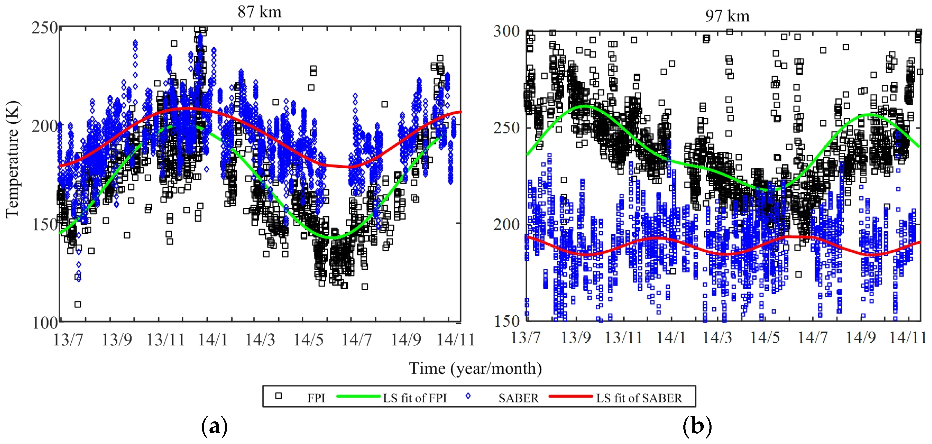
The TIMED satellite is in a circular orbit at 625 km with an inclination of 74.1°. The latitude coverage of TIMED is from 52° N to 83° S or 52° S to 83° N, which means that the satellite can always access the latitude range from 52° S to 52° N. As the orbit of TIMED proceeds slowly, there is a procession of ~12 min in local time between two successive days. Over ~60 days, the satellite samples a full 24 h of local time.
The SABER detector on the TIMED satellite is a limb observation instrument, with kinetic temperature being derived from CO2 infrared limb radiance at tangent altitudes of 15–120 km. In the mesosphere, the effects of non-local thermodynamic equilibrium (NLTE) must be considered in the retrieval scheme [32,33].
In this paper, we use the SABER temperature product of Custom Level 2A, Version 2.0 from January 2002 to February 2015. SABER temperature data are accurate at altitudes of 20–60 km [34]. The NLTE algorithm has been improved substantially in the upper mesosphere and lower thermosphere (UMLT) in versions after 1.06 [26], describing well the characteristics of long-term variations and tides.
Atmospheric variations can be decomposed into several components, including mean waves, tides, and planetary waves [25,35]. In order to eliminate tides and planetary waves so as to obtain more accurate estimates of the zonal mean temperature, a 60-day sliding window with a one-day step is used to deal with the raw data [25]. Since 52° pole-ward observations only exist on alternate yaw cycles, the central latitudes of this paper are extended from 50° S to 50° N, with a resolution of 5°. The vertical profiles are spaced from 20–120 km, with an interval of 1 km.

2.2. FPI Data

The FPI in Kelan observes at wavelength of OH 892.0, OI 557.7, and OI 630.0 nm to derive the nighttime wind and temperature at 87, 97, and 250 km, respectively, and is designed almost the same as the one in Xinglong (40.2° N, 117.4° E) [36]. More details of the mechanism can be found in Yu et al. [30]. Here we use the data from July 2013 to November 2014, and focus on altitudes of 87 and 97 km in the middle atmosphere.
Prior to analysis, the valid data should be selected. The data quality control method is adopted as the following steps: (1) the observed standard deviation is less than 30 m/s for wind and 10 K for temperature at both 87 and 97 km; (2) the absolute wind speed is less than 150 m/s at 87 and 97 km, while the temperature is limited to the range from 100 to 260 K at 87 km and from 150 to 350 K at 97 km; (3) the Grubbs criterion [37] is applied to the daily observations to eliminate outlying ones.

2.3. Analysis Methods

Lomb–Scargle spectral analysis [38] and wavelet analysis [39] can be used to identify the typical oscillations in the middle atmosphere.
The least squares (LS) harmonic fitting method is useful in extracting periodic signals [40]. The main components of the oscillations can be fitted to the following approximation:
T ( t ) = A 0 + A 1 cos ( ω 0 ( t t a o ) ) + A 2 cos ( 2 ω 0 ( t t s a o ) ) + T r e n d t + δ t
Equation (1) suggests that the mean temperature field can be decomposed into five parts. For a given altitude and latitude, T(t) is the zonal mean temperature that varies with time, and A0 is the average climatic state. ω0 = 2π/365 represents the circular frequency of the AO, while the circular frequency of the SAO is 2 ω0. A1 and A2 are the amplitudes of the AO and SAO, and tao and tsao are the phases. Trend is the long-term trend in the mean temperature, and δt is the residual error between the fitting results and the observations. The nonlinear least squares fitting method is applied to determine the parameters of the equation. Using this method, the phase and amplitude of AO and SAO, and the inter-annual variations are derived.

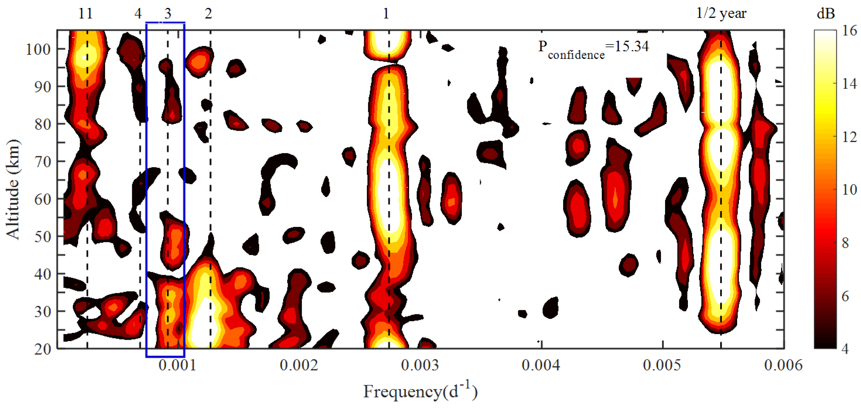
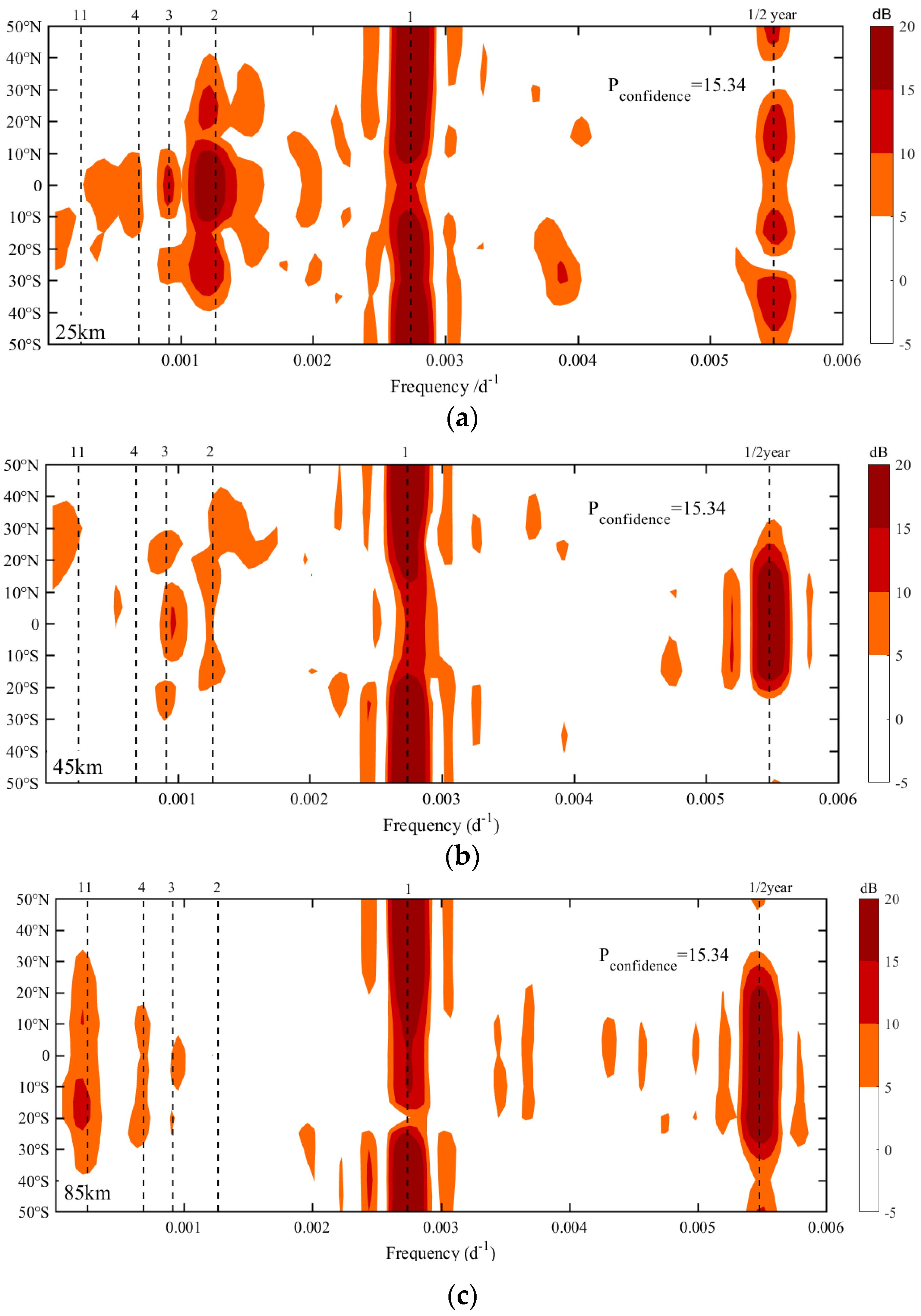
3. Lomb–Scargle Spectral Analysis

Using the method of Lomb–Scargle spectral analysis, several components are identified in the TIMED/SABER temperature. Apart from AO, SAO, and QBO, longer oscillations also exist in the middle atmosphere (e.g., triennial oscillation and the 11-year oscillation). In this section, three typical altitudes are chosen: 25, 45, and 85 km. Figure 1 shows the Lomb–Scargle spectral analysis of the zonal mean temperatures. The shaded areas denote a confidence level of 99%. The power value is defined as PdB = 10log10(P/Pconfidence), where Pconfidence = 15.34 is the corresponding power value obtained for a confidence level of 99%, and P is the power value of the Lomb–Scargle spectral analysis. Figure 1a shows that the AO and QBO are prominent at 25 km. Note that the periodicity of the QBO in the stratosphere is not fixed and is >2 years on average. Hence, the QBO has a period of 26 months in our analysis, as found by Huang et al. (2006) [24]. It is also shown in Figure 1a that the QBO is the main oscillation between 20° S and 20° N in the lower stratosphere, corresponding to the result given by Huang et al. [24,41].
Figure 1b,c show the structure of variations in the upper stratosphere and the mesopause, respectively. The similar features are that the SAO dominates the equatorial regions while the AO is prominent at mid-latitudes. An apparent difference is that the stronger 11-year oscillations exist at 85 km, with a peak around 20° S, although they are weaker than the AOs and SAOs presented. The 11-year oscillations are seen in the mesosphere and lower thermosphere (MLT) and become stronger in the UMLT (figures not shown). Clemesha et al. [42] and Huang et al. [41] indicate that the 11-year oscillations seen in the MLT are highly correlated with the varying ultraviolet flux of the 11-year solar cycle. The four-year oscillation can also be seen at 85 km, with a stronger peak in the southern hemisphere.
It is obvious in Figure 1 that the AO and SAO are the most prominent zonal mean oscillations in the middle atmosphere, and their morphologies are in agreement with previous studies (e.g., [3,4]). In addition, the three-year oscillation signal, which is significant as well as the QBO and SAO, especially at around 45 km over the equatorial region, has attracted our attention. This triennial oscillation (TO) has been discovered in previous studies (e.g., [43]); however, no further work has focused on its morphologies and origins.
Since the climatological overall features of AO were already established many years ago, we will focus on the global structure of SAO and TO using SABER temperature data. Based on the known latitude distributions of those oscillations, we will then study the properties of local variations over Kelan by comparing the FPI data with those from model and TIMED satellite.

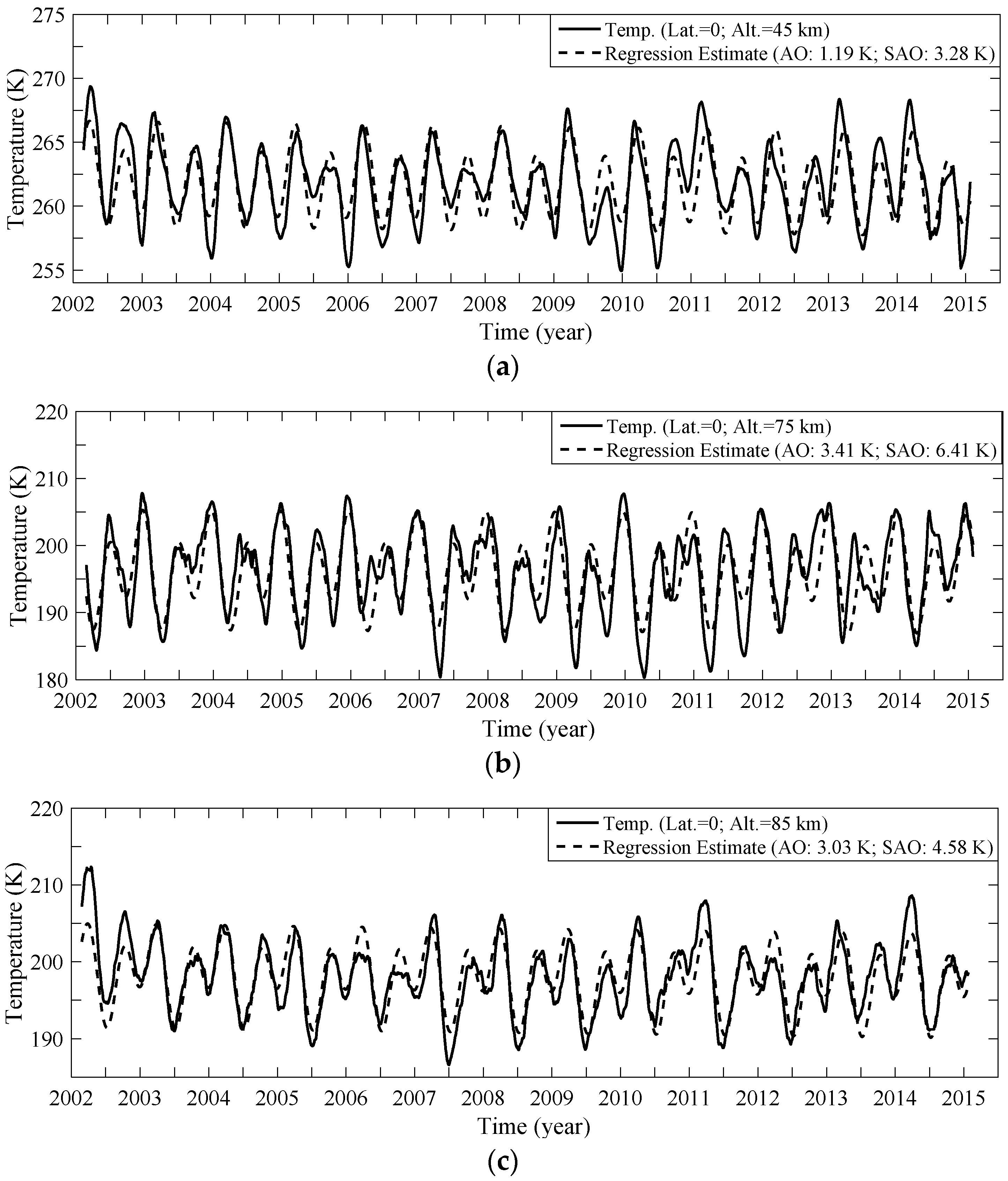
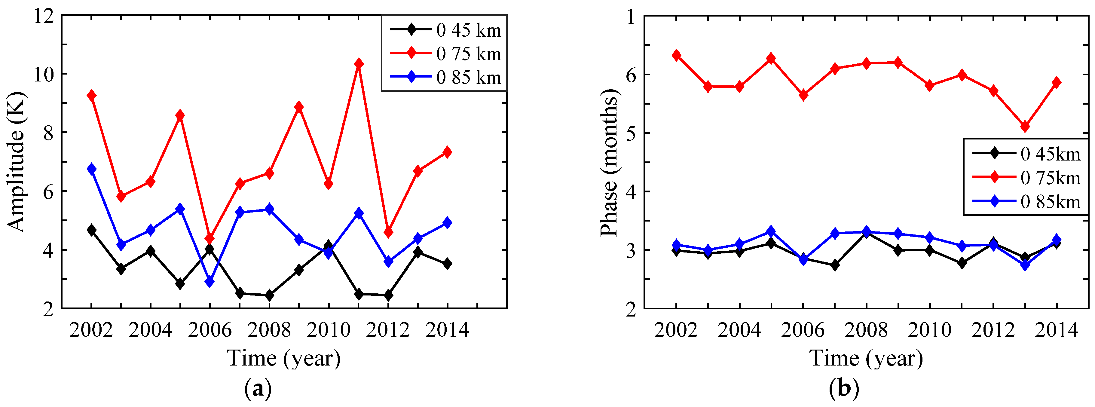
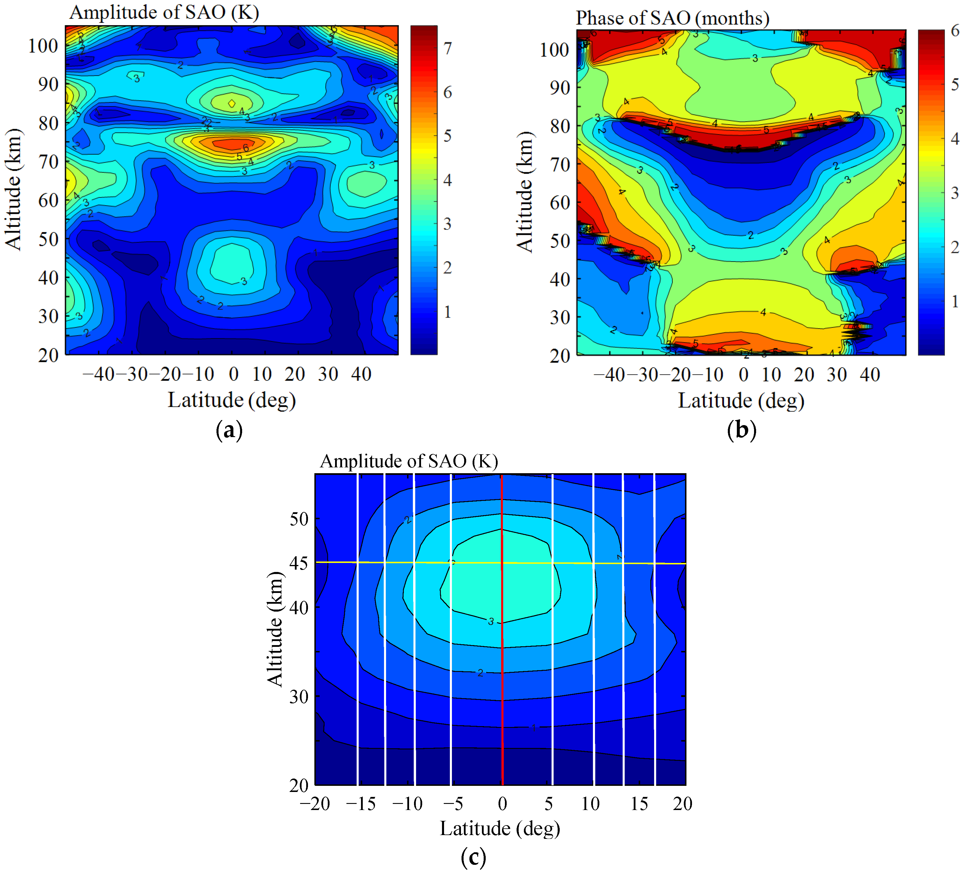
4. Semiannual Oscillation (SAO)

Presented in Figure 2a,b are the amplitude and phase of the SAO based on SABER temperatures. It seems that the SAO amplitude is almost symmetrical with respect to the equator and has a maximum at the equator. However, many former studies reported an asymmetric structure of SSAO with a maximum around 10 degrees in the Southern Hemisphere using rocket observations [7,11,44,45]. Moreover, Garcia et al. [45] show that the SSAO was strongly influenced by a stronger cross-equatorial advection of mean easterly winds from the Southern Hemisphere summer than that from the Northern Hemisphere winter on a zonal mean basis. This asymmetry between the hemispheres could reflect the meridional asymmetry of the SSAO amplitude in the zonal wind field. As mentioned before, zonal mean winds are intimately connected with meridional temperature gradients through the thermal wind balance. Thus, the asymmetric structure is expected to show in the temperature field. In order to explain the discrepancy, we present in Figure 2c the detail structure of amplitude at stratosphere around the equator. It is shown in Figure 2c that although the meridional structure of the temperature SSAO amplitude seems to be fairly symmetric at a glance, there actually exists subtle asymmetricity in the upper stratosphere. The maximum amplitude of the SSAO is observed around 45 km, so it is appropriate to examine the meridional structure at 45 km, under the consideration of the thermal wind balance. The vertical lines showing contour intervals are added to the figure in the equatorial region of both hemispheres, which could show a discernable difference of contour intervals between the hemispheres, i.e., narrower intervals in the equatorial Southern Hemisphere, especially in 5–15 degrees of latitude. Because of a small Coriolis parameter in the equatorial region, such a small difference in the temperature field could be magnified in the zonal wind field, which would make larger SSAO amplitudes in zonal winds, leading to the asymmetric meridional structure of the zonal wind SSAO amplitude with respect to the equator.
In the tropical regions, the stratospheric SAO has a peak of >3 K in the 40–50 km layer. The mesospheric SAO has two amplitude maxima: one >6 K at 75 km, and the other ~4.5 K at 85 km. After diminishing between 20°–40°, the amplitude increases again at latitudes pole-ward of 40°. It seems that the extratropical SAO is stronger in SH than in NH. The differences in phase progression and amplitude distribution indicate that the mechanism of extratropical SAO is different from the tropical SAO. The extratropical SAO is probably due to the occurrence of sudden warming events and the enhancement of meridional circulation associated with strong wave forcing during winter periods [7].
The time series of SABER temperatures from January 2002 to February 2015 at the altitudes where the SAO is strongest is presented in Figure 3. There are seasonal asymmetries in SAO: the SAOs at 45 km and 85 km have larger maxima at spring equinoxes than those at autumn equinoxes, while the SAO at 75 km has larger minima at spring equinoxes. This is similar to the results given by Garia et al. [45] except at 85 km, where the SAO amplitude derived from SME (Solar Mesosphere Explorer) satellite is considered to contaminate by the diurnal tide. The phases of the SAO in the upper stratosphere (45–50 km) are around the equinox and are mostly in phase with those in the UMLT. The phase reversal between 75 and 85 km is linked to the lower mesospheric inversion layers, as will be discussed in detail in the next section.
We now consider the wavelet spectrum at the equator. Figure 4 shows that SAO is the dominant oscillation at the equator. In addition, comparing with Figure 1, the TO can be seen to have been a salient oscillation at 45 and 85 km throughout most of 2002–2015.
The variations of SAO amplitudes and phases from 2002 to 2014 are shown in Figure 5. Figure 5a shows that the amplitudes at 75 and 85 km have similar trends, with maximum amplitudes in 2002, 2005, and 2011; both exhibit a period of ~3 years. The SAO phase shows relatively weak inter-annual variation.

5. The Lower Mesospheric Inversion Layer (MIL)

The term mesospheric inversion layer (MIL) is defined from the fact that the lapse rate of the temperature is positive at specific layers in the mesosphere. Studies have revealed that the MIL can be divided into two sub-layers: the lower and the upper MILs at approximately 75 and 90 km, respectively (e.g., [23,46]). The following discussion is concerned with the lower MIL.
In order to extract the lower MILs from the background temperature, we use a method analogous to that of Gan et al. [47]. The 60-day averaged vertical temperature profiles are used to identify the local maximum and minimum nodes at 65–85 km. The largest difference between successive such nodes is then identified as the amplitude of the lower MIL. Note that the 60-day average temperature data are used here to investigate the influence of background temperature to the MIL.
The temporal variation of the lower MIL amplitude is shown in Figure 6. The largest amplitudes of the lower MIL occur in regions within 15° of the equator. The amplitude peaks are largest during almost every equinox, and contain evident semi-annual cycles. Note that the peaks at the spring equinox appear to be more robust than those at the autumn one.
Figure 7 presents the variation of background zonal mean temperature at the equator. The temperature increases during each spring and autumn equinox between 75 and 85 km. This increase is synchronous with the existence of MIL amplitude maxima, indicating that the structure of the mesospheric SAO may cause lower tropical MIL.
The contribution of SAO to the MIL is analyzed quantitatively below. As shown in Section 4 that SAO is strong at both 75 and 85 km. These altitudes correspond to the bottom (75 km) and top (85 km) of the lower MIL. Figure 8 shows that the amplitude reaches peaks at 75 and 85 km, and the respective phases are around both solstices and both equinoxes. The SAO phase changes rapidly from 75 to 85 km. This feature may cause the temperature to increase between 75 and 85 km at each equinox, resulting in a temperature inversion of ~11 K at the equator on average. The phenomenon that stronger MIL amplitudes are at spring equinox than at autumn equinox can be explained by the seasonal asymmetries at both 75 and 85 km described in Section 4. This is not pointed out in previous studies (e.g., [25,47]).

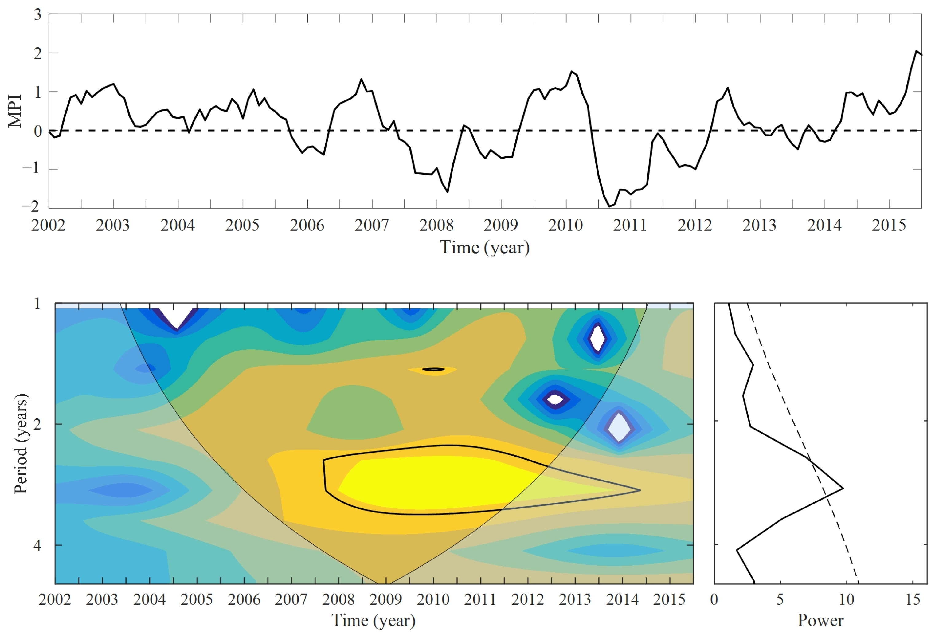
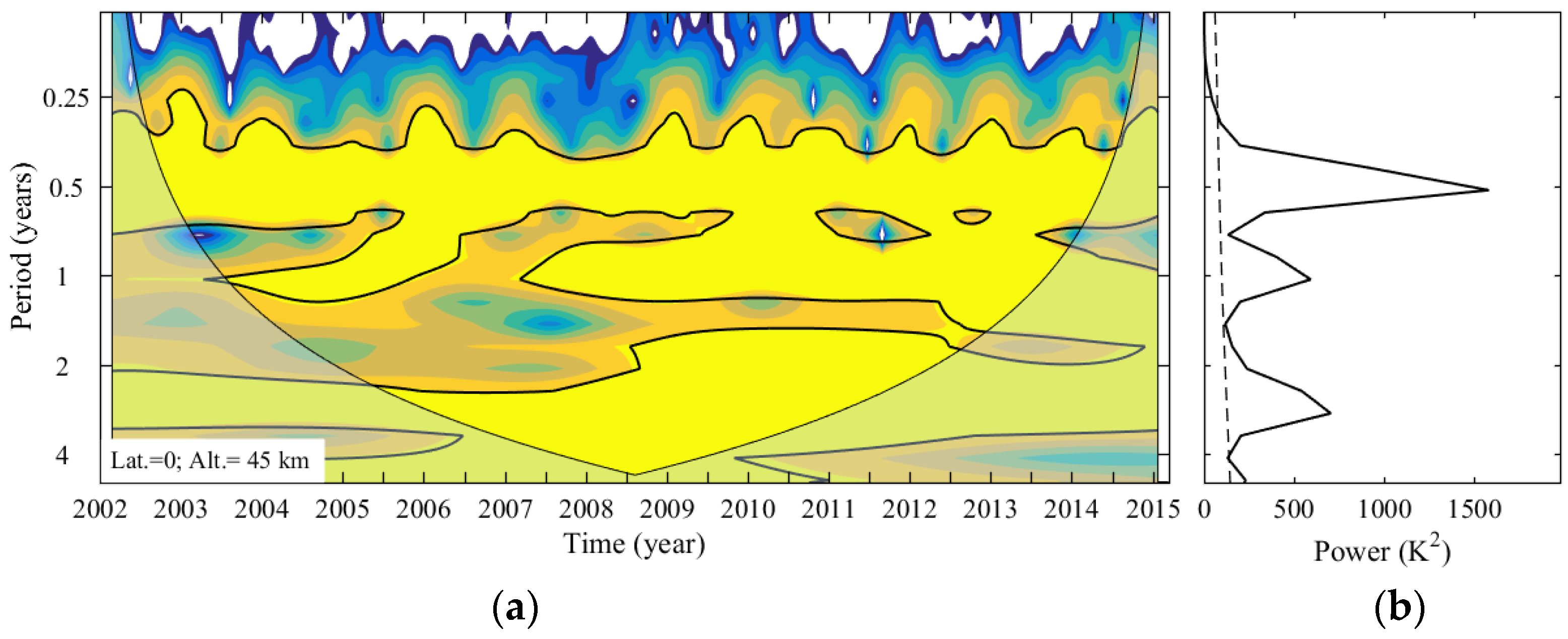
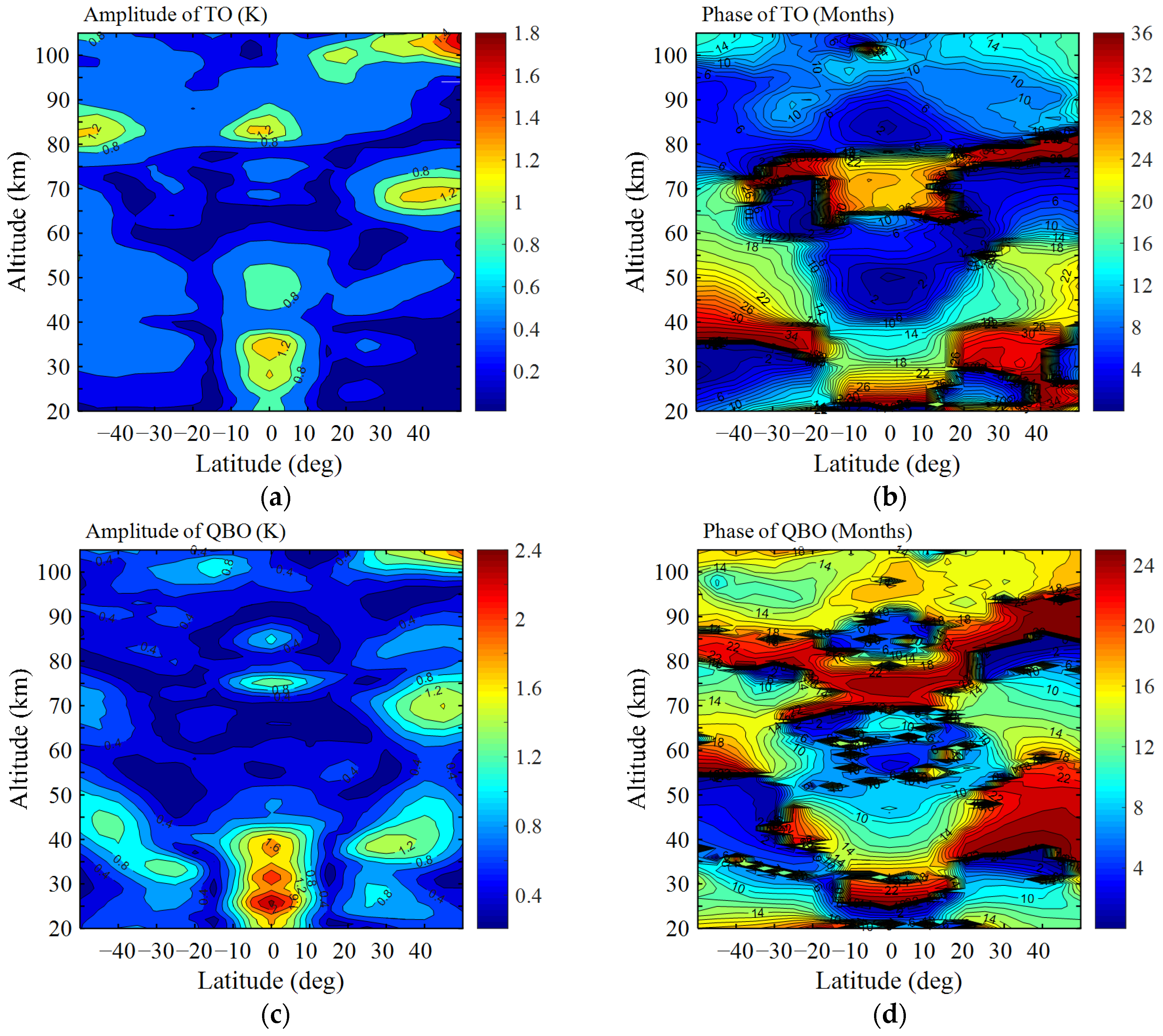
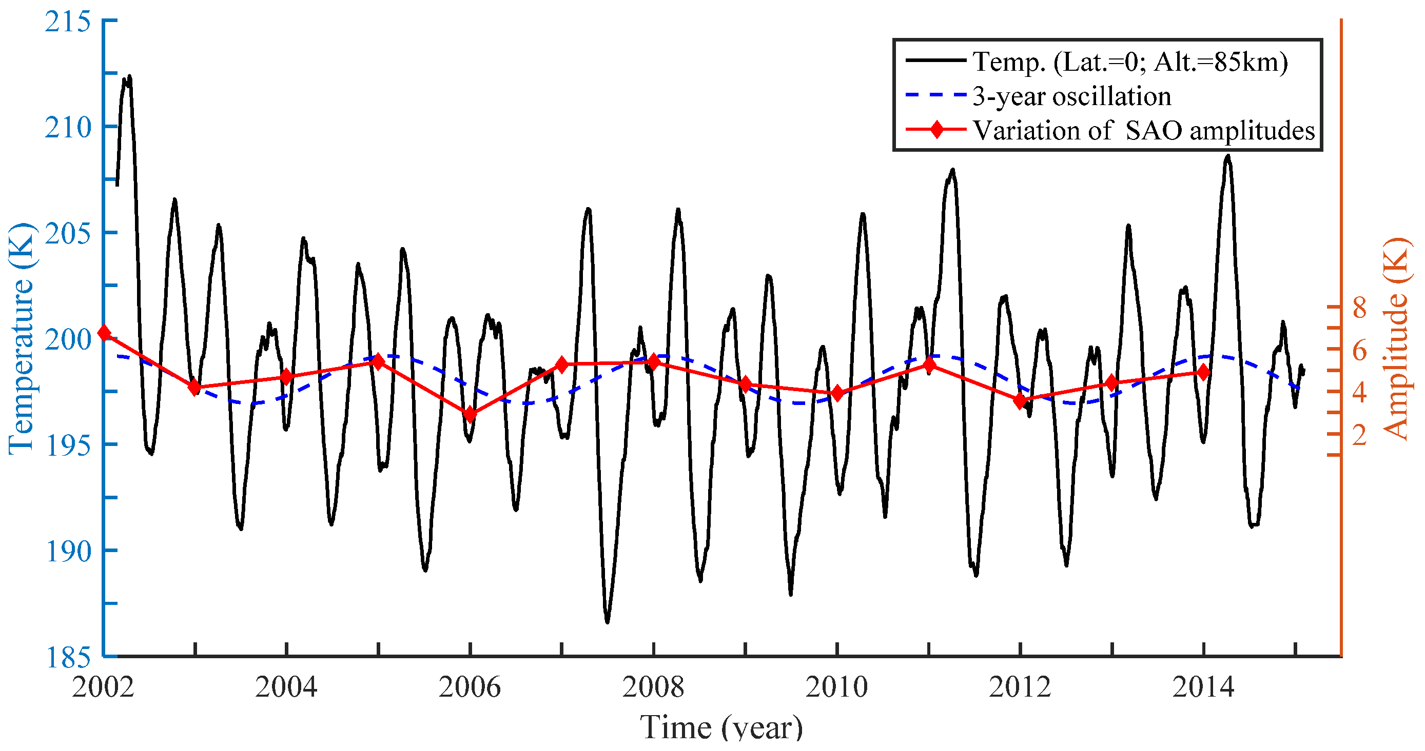
6. The Triennial Oscillation (TO)

As discussed in previous sections, the TO is also prominent in the mesosphere, especially in the tropical region. As illustrated in the blue-lined box of Figure 9, the strong signal of TO can be seen in most of the stratosphere and ~85 km in the mesosphere at the equator. It is well known that a period of the QBO varies from 22 to 34 months with an average period of about 28 months [19]. The longer wing of the variation, 34 months, is very close to the period of the TO. We first give an analysis of the relationship between QBO and TO.
The amplitude and phase of TO (36 months) and QBO (26 months) as a function of altitude and latitude are extracted from the residual error in Equation (1). As can be seen in Figure 10, the amplitude of the TO is no more than 2 K. In the tropical region, the TO has three amplitude maxima, two in the stratosphere (35 km and 45 km) and one in the mesosphere (85 km). The amplitudes are ~1.2 K, ~0.8 K, and ~1.2, K respectively. The phases at 45 km and 85 km are ~2nd month, while the phase at 35 km is ~14th month. Comparing Figure 10b,d, we find that the phase structure of TO shows a similar feature to that of QBO, especially around the equator. Moreover, the amplitude of TO and QBO both show maxima at the stratosphere (30–40 km) and upper mesosphere (~85 km) at the equator. Based on the discussion above, we believe that the spectral peak of TO is probably a sub-peak of the QBO and is due to modulation of the QBO.
As mentioned in Section 4, three-year periodicities SAO are seen at 75 and 85 km over the equator in Figure 5. Is it related to the TO detected in the background temperature? Figure 11 shows the interannual variation of amplitudes of SAO and the variation of TO at 85 km at the equator. It seems that the two time series are in phase and share the similar amplitudes. However, the three-year periodicities in the SAO at 75 km over the equator are out of phase with the TO (figures not shown). This suggests that there may be potential interaction of the TO with SAO, mainly at ~85 km at the equator.
Several studies have revealed that the El Nino–Southern Oscillation (ENSO) can influence the tropical stratospheric temperature [48,49,50]. The ENSO variations can be characterized by the Multivariate ENSO Index (MEI) [51]. As seen in Figure 12, the MEI has a significant three-year oscillation from 2008 to 2014. So, is ENSO related to the TO in the middle atmosphere? The ENSO signals can influence the middle atmosphere by means of planetary wave. In the tropical region, the rhythmic warming and cooling signal of ENSO are usually accompanied by the opposite sign in the lower stratospheric zonal mean temperature [49]. However, this ENSO-related influence is not discernible above ~23 km at the equator [48,52], where the TO is significant. Above all, we believe that the ENSO signal may also modulate the amplitude of the TO, mainly in the lower stratosphere.

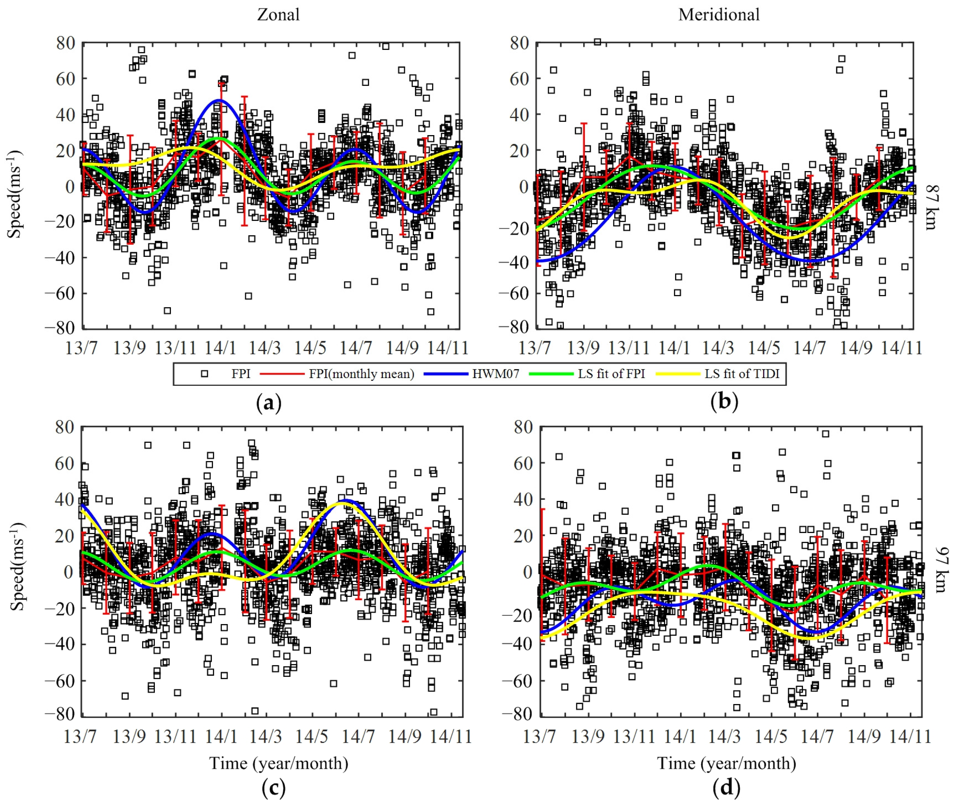
7. The Long-Term Variations Observed by FPI

In this section, we will give an analysis of the long-term variations based on the FPI data from July 2013 to November 2014. Comparisons have been made between the FPI wind products and those from horizontal wind models and meteor radar, indicating that the FPI is a reliable instrument in the wind measurements [30,31]. Since our data are limited, we will mainly focus on the nighttime long-term variations of AO and SAO.
Note that the data from the Horizontal Wind Model (HWM07) [21], and TIMED Doppler Interferometer (TIDI) product provided by NCAR version 0307A [53] are also used to assess the results from FPI wind. The three-hour Ap index is applied in HWM07, and the data from TIDI is processed similarly to that of SABER to derive 60-day zonal mean winds. It is the midnight winds (00:00 LT ± 2 h) that are chosen to compare with those from HWM07, since there are more data at midnight. The LS fitting is applied to obtain the amplitude and phase of AO and SAO. The results are shown in Figure 13 and Table 1.
The monthly mean FPI zonal winds are consistent with those from HWM07 at 87 and 97 km, and they both exhibit similar phase of AO and SAO. However, as indicated in Figure 13 and Table 1, the amplitudes of zonal wind derived from HWM07 are generally larger than those from FPI. There are different results in meridional winds. The FPI meridional winds are similar in amplitude to those from HWM07, although the HWM07 results are a bit larger. Nevertheless, it is shown that the phases of FPI lag marginally behind those of HWM07. The discrepancies between FPI and HWM07 winds may lie in the fact that (1) HWM07 has not included the ground-based measurements over China [21] and the applicability of it over China remains a problem; and (2) the fact that airglow layer is relatively thicker than the vertical wavelength of tides may induce weak amplitudes of FPI [54].
By comparing the nighttime winds from FPI and the zonal mean winds at the same latitude (38.7° N) from TIDI, we find that the FPI and TIDI winds share similar AO and SAO phases in many cases. Their amplitudes, however, are generally different. This could be due in part to the difference in data sampling and data processing procedures, but even more importantly because of tidal aliasing. The TIDI results are derived from 60-day zonal mean with removal of tides; however, the results of FPI are derived from nighttime wind, which will be influenced by the strong tides in MLT region. The tidal amplitudes may influence those of nighttime AO and SAO depending on the tidal phase [27].
Note that the FPI temperature over Kelan has never been evaluated before. In order to evaluate its accuracy, the nighttime SABER temperature over Kelan is obtained in a box of 6° × 6° with respect to the central latitude and altitude at 87 and 97 km. The results are presented in Figure 14 and Table 2. It is shown that the difference between FPI and SABER is large at 97 km in both phase and amplitude. At 87 km, their phases are similar; however, the amplitudes derived from FPI are nearly twice those from SABER. Since the accuracy of nighttime SABER data has been confirmed by comparing several ground-based measurements in the MLT region [26], we believe that the algorithm to derive FPI temperature needs imporvements.

8. Conclusions

Basing on SABER 2.0 temperature data from January 2002 to February 2015, and ground-based FPI data from July 2013 to November 2014, we mainly studied the properties of long-term variations in the middle atmosphere. The main conclusions are presented as below:
The SAO can be discovered in both tropical and mid-latitude regions. The differences in phase progression and amplitude distribution indicate that the mechanism of extratropical SAO is different from the tropical SAO. The SAO in the tropical areas shows three amplitude maxima: one in the stratosphere (45 km) and two in the mesosphere (75 and 85 km). The seasonal asymmetries are prominent in SAO: the SAOs at 45 km and 85 km have larger maxima at spring equinoxes than those at autumn equinoxes, while the SAO at 75 km has larger minima at spring equinoxes. A phase inversion can be identified between 75 and 85 km. The amplitudes at both 75 and 85 km contain prominent interannual variations that have similar trends, each exhibiting a period of ~3 years.
The SAO is closely associated with the lower MIL. The largest amplitudes of the lower MIL fall in the regions within 15° of the equator. The amplitude peaks are largest during almost every equinox, showing prominent semi-annual cycles. Note that the phase inversion between 75 and 85 km may cause the 11-K enhancement in the background temperature on average, with stronger enhancement at the spring equinox than at the autumn equinox. The difference between the two equinoxes can be explained by the seasonal asymmetries at 75 and 85 km.
The TO is significant in tropical regions. There are three amplitude maxima of the TO at the equator: two in the stratosphere (35 km and 45 km) and one in the mesosphere (85 km). Results show that the TO has a close relationship with QBO. The spectral peak of TO is probably a sub-peak of the QBO and is due to modulation of the QBO. The three-year periodicities in the SAO match well with the TO at 85 km at equator, indicating a potential interaction of he TO with SAO there. The relationship between ENSO and TO has also been discussed. Results are that the ENSO signal may modulate the amplitude of the TO, mainly in the lower stratosphere.
The amplitude and phase of AO and SAO from FPI wind data have been compared with those from HWM07 and TIDI. Generally, the results of FPI data consist well with HWM07, though amplitudes are larger in HWM07, and the phases of FPI marginally lag behind those of HWM07 in meridional winds. The comparison between FPI and TIDI winds shows a relatively large discrepancy. Since the FPI results are for nighttime only, the strong tidal amplitudes in MLT may influence those of nighttime AO and SAO depending on the tidal phase, which may lead to the discrepancy. The quality of FPI temperature data is evaluated by comparing with those from SABER. Results show that the algorithm to derive FPI temperature needs improvements.

Acknowledgments

The SABER data used here were provided by the TIMED/SABER team, and we would like to acknowledge their contribution to this work. The study was partly supported by the National Natural Science Foundation of China (Grant No. 41375028), and the National Natural Science Foundation of Jiangsu, China (Grant No. BK20151446).

Author Contributions

Shudao Zhou, Hanqing Shi, and Zheng Sheng conceived and designed the experiments; Yiyao Zhang, Zhiqiang Fan, and Huadong Du performed the experiments; Yiyao Zhang and Weilai Shi analyzed the data; Yiyao Zhang wrote the paper; Hanqing Shi gave important suggestions for analyzing FPI data.

Conflicts of Interest

The authors declare no conflicts of interest.

References

  1. Swinbank, R.; Ortland, D.A. Compilation of wind data for the Upper Atmosphere Research Satellite (UARS) Reference Atmosphere Project. J. Geophys. Res. 2003, 108, 1703–1708. [Google Scholar] [CrossRef]
  2. Fleming, E.L.; Chandra, S.; Barnett, J.J.; Corney, M. Zonal mean temperature, pressure, zonal wind and geopotential height as functions of latitude. Adv. Space Res. 1990, 10, 11–59. [Google Scholar] [CrossRef]
  3. Remsberg, E.E.; Bhatt, P.P.; Deaver, L.E. Seasonal and longer-term variations in middle atmosphere temperature from HALOE on UARS. J. Geophys. Res. 2002, 107, ACL 18:1–ACL 18:13. [Google Scholar] [CrossRef]
  4. Xu, J.; Liu, H.L.; Yuan, W.; Smith, A.K.; Roble, R.G.; Mertens, C.J.; Russell, J.M.; Mlynczak, M.G. Mesopause structure from Thermosphere, Ionosphere, Mesosphere, Energetics, and Dynamics (TIMED)/Sounding of the Atmosphere Using Broadband Emission Radiometry (SABER) observations. J. Geophys. Res. 2007, 112, 139–155. [Google Scholar] [CrossRef]
  5. Mayr, H.G.; Mengel, J.G.; Chan, K.L.; Huang, F.T. Middle atmosphere dynamics with gravity wave interactions in the numerical spectral model: Zonal-mean variations. J. Atmos. Solar-Terr. Phys. 2010, 72, 807–828. [Google Scholar] [CrossRef]
  6. Holton, J.R.; Wehrbein, W.M. A numerical model of the zonal mean circulation of the middle atmosphere. Pure Appl. Geophys. 1980, 118, 284–306. [Google Scholar] [CrossRef]
  7. Hirota, I. Observational evidence of the semiannual oscillation in the tropical middle atmosphere—A review. Pure Appl. Geophys. 1980, 118, 217–238. [Google Scholar] [CrossRef]
  8. Meyer, W.D. A diagnostic numerical study of the semiannual variation of the zonal wind in the tropical stratosphere and mesosphere. J. Atmos. Sci. 1970, 27, 820–830. [Google Scholar] [CrossRef]
  9. Hamilton, K. Dynamics of the stratospheric semi-annual oscillation. J. Meteorol. Soc. Jpn. 1986, 64, 227–244. [Google Scholar]
  10. Hamilton, K.; Wilson, R.J.; Mahlman, J.D.; Umscheid, L.J. Climatology of the SKYHI troposphere-stratosphere-mesosphere general circulation model. J. Atmos. Sci. 1995, 52, 5–43. [Google Scholar] [CrossRef]
  11. Hopkins, R.H. Evidence of polar-tropical coupling in upper stratospheric zonal wind anomalies. J. Atmos. Sci. 1975, 32, 712–719. [Google Scholar] [CrossRef]
  12. Hirota, I. Equatorial waves in the upper stratosphere and mesosphere in relation to the semiannual oscillation of the zonal wind. J. Atmos. Sci. 1978, 35, 714–722. [Google Scholar] [CrossRef]
  13. Andrews, D.G.; Holton, J.R.; Leovy, C.B. Middle Atmosphere Dynamics; Elsevier: New York, NY, USA, 1987; p. 489. [Google Scholar]
  14. Richter, J.H.; Garcia, R.R. On the forcing of the Mesospheric Semi-Annual Oscillation in the Whole Atmosphere Community Climate Mode. Geophys. Res. Lett. 2006, 33, 313–324. [Google Scholar] [CrossRef]
  15. Dunkerton, T.J. Theory of the mesopause semiannual oscillation. J. Atmos. Sci. 1982, 39, 2681–2690. [Google Scholar] [CrossRef]
  16. Sassi, F.; Garcia, R.R. The role of equatorial waves forced by convection in the tropical semiannual oscillation. J. Atmos. Sci. 1997, 54, 1925–1942. [Google Scholar] [CrossRef]
  17. Lindzen, R.S.; Holton, J.R. A theory of the quasi-biennial oscillation. J. Atmos. Sci. 1968, 25, 1095–1107. [Google Scholar] [CrossRef]
  18. Plumb, R.A. The interaction of two internal waves with the mean flow: Implications for the theory of the quasi-biennial oscillation. J. Atmos. Sci. 1977, 34, 1847–1858. [Google Scholar] [CrossRef]
  19. Baldwin, M.P.; Gray, L.J.; Dunkerton, T.J.; Hamilton, K.; Haynes, P.H.; Randel, W.J.; Holton, J.R.; Alexander, M.J.; Hirota, I.; Horinouchi, T.; et al. The quasi-biennial oscillation. Rev. Geophys. 2001, 39, 179–229. [Google Scholar] [CrossRef]
  20. Zhu, X.; Yee, J.H.; Cai, M.; Swartz, W.H.; Coy, L.; Aquila, V.; Garcia, R.; Talaat, E.R. Diagnosis of Middle-Atmosphere Climate Sensitivity by the Climate Feedback–Response Analysis Method. J. Atmos. Sci. 2016, 73, 3–23. [Google Scholar] [CrossRef]
  21. Drob, D.P.; Emmert, J.T.; Crowley, G.; Picone, J.M.; Shepherd, G.G.; Skinner, W.; Meriwether, J.W. An empirical model of the Earth’s horizontal wind fields: HWM07. J. Geophys. Res. 2008, 113, A12304. [Google Scholar] [CrossRef]
  22. Mingalev, I.V.; Mingalev, V.S.; Mingaleva, G.I. Numerical Simulation of the Global Neutral Wind System of the Earth’s Middle Atmosphere for Different Seasons. Atmosphere 2012, 3, 213–228. [Google Scholar] [CrossRef]
  23. Clancy, R.T.; Rusch, D.W.; Callan, M.T. Temperature minima in the average thermal structure of the middle mesosphere (70–80 km) from analysis of 40- to 92-km SME global temperature profiles. J. Geophys. Res. 1994, 99, 19001–19020. [Google Scholar] [CrossRef]
  24. Huang, F.T.; Mayr, H.G.; Reber, C.A.; Russell, J.M.; Mlynczak, M.; Mengel, J.G. Stratospheric and mesospheric temperature variations for the quasi-biennial and semiannual (QBO and SAO) oscillations based on measurements from SABER (TIMED) and MLS (UARS). Ann. Geophys. 2006, 24, 2131–2149. [Google Scholar] [CrossRef]
  25. Xu, J.; Smith, A.K.; Yuan, W.; Liu, H.L.; Qian, W.; Mlynczak, M.G.; Russell, J.M. Global structure and long-term variations of zonal mean temperature observed by TIMED/SABER. J. Geophys. Res. 2007, 112, 177–180. [Google Scholar] [CrossRef]
  26. Remsberg, E.E.; Marshall, B.T.; Garcia-Comas, M.; Krueger, D.; Lingenfelser, G.S.; Martin-Torres, J.; Mlynczak, M.G.; Russell, J.M.; Smith, A.K.; Zhao, Y.; Brown, C. Assessment of the quality of the Version 1.07 temperature-versus-pressure profiles of the middle atmosphere from TIMED/SABER. J. Geophys. Res. 2008, 113, 1641–1653. [Google Scholar] [CrossRef]
  27. Dou, X.; Li, T.; Xu, J.; Liu, H.L.; Xue, X.; Wang, S.; Leblanc, T.; Mcdermid, I.S.; Hauchecorne, A.; Keckhut, P. Seasonal oscillations of middle atmosphere temperature observed by Rayleigh lidars and their comparisons with TIMED/SABER observations. J. Geophys. Res. 2009, 114, 311. [Google Scholar] [CrossRef]
  28. Hocking, W.K. Temperatures Using radar-meteor decay times. Geophys. Res. Lett. 1999, 26, 3297–3300. [Google Scholar] [CrossRef]
  29. Sheng, Z.; Jiang, Y.; Wan, L.; Fan, Z.Q. A Study of Atmospheric Temperature and Wind Profiles Obtained from Rocketsondes in the Chinese Midlatitude Region. J. Atmos. Ocean. Technol. 2015, 32, 722–735. [Google Scholar] [CrossRef]
  30. Yu, T.; Huang, C.; Zhao, G.; Mao, T.; Wang, Y.; Zeng, Z.; Wang, J.; Xia, C. A preliminary study of thermosphere and mesosphere wind observed by Fabry-Perot over Kelan, China. J. Geophys. Res. 2014, 119, 4981–4997. [Google Scholar] [CrossRef]
  31. Yao, X.; Yu, T.; Zhao, B.; Yu, Y.; Liu, L.; Ning, B.; Wan, W. Climatological modeling of horizontal winds in the mesosphere and lower thermosphere over a mid-latitude station in China. Adv. Space Res. 2015, 56, 1354–1365. [Google Scholar] [CrossRef]
  32. Mertens, C.J.; Mlynczak, M.G.; Manuel, L.P.; Wintersteiner, P.P.; Picard, R.H.; Winick, J.R.; Gordley, L.L.; Russell, J.M. Retrieval of Mesospheric and Lower Thermospheric Kinetic Temperature from Measurements of CO2 15 Micrometers Earth Limb Emission under Non-LTE Conditions. Geophys. Res. Lett. 2001, 28, 1391–1394. [Google Scholar] [CrossRef]
  33. Mertens, C.J.; Schmidlin, F.J.; Goldberg, R.A.; Remsberg, E.E.; Dean, P.W.; Russell, J.M.; Mlynczak, M.G.; Manuel, L.P.; Wintersteiner, P.P.; Picard, R.H. SABER observations of mesospheric temperatures and comparisons with falling sphere measurements taken during the 2002 summer MaCWAVE campaign. Geophys. Res. Lett. 2004, 31, 445–446. [Google Scholar] [CrossRef]
  34. Fan, Z.Q.; Sheng, Z.; Shi, H.Q.; Yi, X.; Jiang, Y.; Zhu, E.Z. Comparative Assessment of COSMIC Radio Occultation Data and TIMED/SABER Satellite Data over China. J. Appl. Meteorol. Climatol. 2015, 54, 1931–1943. [Google Scholar] [CrossRef]
  35. Mcdonald, A.J.; Baumgaertner, A.J.G.; Fraser, G.J.; George, S.E.; Marsh, S. Empirical Mode Decomposition of the atmospheric wave field. Ann. Geophys. 2007, 25, 255–270. [Google Scholar] [CrossRef]
  36. Yuan, W.; Xu, J.Y.; Ma, R.P.; Wu, Q.; Jiang, G.Y.; Gao, H.; Liu, X.; Chen, S.Z. First observation of mesospheric and thermospheric winds by a Fabry-Perot interferometer in China. Chin. Sci. Bull. 2010, 55, 4046–4051. [Google Scholar] [CrossRef]
  37. Grubbs, F.E. Procedures for detecting outlying observations in samples. Technometrics 1969, 11, 1–21. [Google Scholar] [CrossRef]
  38. Press, W.H.; Teukolsky, S.A.; Vetterling, W.T.; Flannery, B.P. Numerical Recipes in Fortran 77, 2nd ed.; Cambridge University Press: New York, NY, USA, 1992; pp. 569–577. [Google Scholar]
  39. Torrence, C.; Compo, G.P. A Practical Guide to Wavelet Analysis. Bull. Am. Meteorol. Soc. 1998, 79, 61–78. [Google Scholar] [CrossRef]
  40. Lomb, N.R. Least-squares frequency analysis of unequally spaced data. Astrophys. Space Sci. 1976, 39, 447–462. [Google Scholar] [CrossRef]
  41. Huang, F.T.; Mayr, H.G.; Russell, J.M., III; Mlynczak, M.G. Ozone and temperature decadal responses to solar variability in the mesosphere and lower thermosphere, based on measurements from SABER on TIMED. Ann. Geophys. 2016, 34, 29–40. [Google Scholar] [CrossRef]
  42. Clemesha, B.; Takahashi, H.; Simonich, D.; Gobbi, D.; Batista, P. Experimental evidence for solar cycle and long-term change in the low-latitude MLT region. J. Atmos. Terr. Phys. 2005, 67, 191–196. [Google Scholar] [CrossRef]
  43. Kane, R.P.; Buriti, R.A. Latitude and Altitude Dependence of the Interannual Variability and Trends of Atmospheric Temperatures. Pure Appl. Geophys. 1997, 149, 775–792. [Google Scholar] [CrossRef]
  44. Belmont, A.D.; Dartt, D.G.; Nastrom, G.D. Periodic variations in stratospheric zonal wind from 20 to 65 km, at 80 N to 70 S. Q. J. R. Meteorol. Soc. 1974, 100, 203–211. [Google Scholar]
  45. Garcia, R.R.; Dunkerton, T.J.; Lieberman, R.S.; Vincent, R.A. Climatology of the semiannual oscillation, of the tropical middle atmosphere. J. Geophys. Res. 1997, 102, 26019–26032. [Google Scholar] [CrossRef]
  46. Meriwether, J.W.; Gardner, C.S. A review of the mesosphere inversion layer phenomenon. J. Geophys. Res. 2000, 105, 12405–12416. [Google Scholar] [CrossRef]
  47. Gan, Q.; Zhang, S.D.; Yi, F. TIMED/SABER observations of lower mesospheric inversion layers at low and middle latitudes. J. Geophys. Res. 2012, 117, 134–142. [Google Scholar] [CrossRef]
  48. Reid, G.C. Seasonal and interannual temperature variations in the tropical stratosphere. J. Geophys. Res. 1994, 99, 18923–18932. [Google Scholar] [CrossRef]
  49. Randel, W.J.; Garcia, R.R.; Calvo, N.; Dan, M. ENSO influence on zonal mean temperature and ozone in the tropical lower stratosphere. Geophys. Res. Lett. 2009, 36, 172–173. [Google Scholar] [CrossRef]
  50. Seidel, D.J.; Li, J.; Mears, C.; Moradi, I.; Nash, J.; Randel, W.J.; Saunders, R.; Thompson, D.W.J.; Zou, C.Z. Stratospheric temperature changes during the satellite era. J. Geophys. Res. 2016, 121, 664–681. [Google Scholar] [CrossRef]
  51. Wolter, K.; Timlin, M.S. El Nino/Southern Oscillation behaviour since 1871 as diagnosed in an extended multivariate ENSO index (MEI.ext). Int. J. Climatol. 2011, 31, 1074–1087. [Google Scholar] [CrossRef]
  52. Garcia-Herrera, R.; Calvo, N.; Garcia, R.R.; Giorgetta, M.A. Propagation of ENSO temperature signals into the middle atmosphere: A comparison of two general circulation models and ERA-40 reanalysis data. J. Geophys. Res. 2006, 111, 831–846. [Google Scholar] [CrossRef]
  53. Xu, J.Y.; Smith, A.K.; Liu, H.L.; Yuan, W.; Wu, Q.; Jiang, G.; Mlynczak, M.G.; Russell, J.M.; Franke, S.J. Seasonal and quasi-biennial variations in the migrating diurnal tide observed by Thermosphere, Ionosphere, Mesosphere, Energetics and Dynamics (TIMED). J. Geophys. Res. 2009, 114, 267–275. [Google Scholar] [CrossRef]
  54. Yuan, W.; Liu, X.; Xu, J.Y.; Zhou, Q.; Jiang, G.; Ma, R. FPI observations of nighttime mesospheric and thermospheric winds in China and their comparisons with HWM07. Ann. Geophys. 2013, 31, 1365–1378. [Google Scholar] [CrossRef]
Figure 1. Lomb–Scargle spectral analysis of zonal mean temperature. (a) for 25 km; (b) for 45 km; (c) for 85 km.
Atmosphere 08 00007 g001
Figure 2. Distribution of (a) the amplitude (K); (b) phase (months) and (c) the amplitude at stratosphere around equator of SAO. Contour intervals are 0.5 K and 0.5 month.
Atmosphere 08 00007 g002
Figure 3. Time series of zonal mean temperature at the equator. (a) for 45 km; (b) for 75 km; (c) for 85 km.
Atmosphere 08 00007 g003
Figure 4. The wavelet power spectrum and the global wavelet spectrum at the equator (a,b) for 45 km; (c,d) for 75 km; and (e,f) for 85 km. Note that the Morlet wavelet normalized by standard deviation is used here. The thick-contour-enclosed regions are the places where there is greater than 95% confidence for a red-noise process with a lag-1 coefficient of 0.72. Transparent regions indicate the ‘cone of influence’, where the edge effects become important, which means that anything in this region is dubious. The global wavelet spectrum is on the right side of the wavelet power spectrum. The dashed line is the 95% confidence level for the global wavelet spectrum.
Atmosphere 08 00007 g004aAtmosphere 08 00007 g004b
Figure 5. Variations of (a) the amplitudes and (b) phases of the SAO at the equator at 45, 75, and 85 km.
Atmosphere 08 00007 g005
Figure 6. Zonal mean temperature amplitudes of the lower MIL, 2002–2015. Contour interval is 3 K.
Atmosphere 08 00007 g006
Figure 7. Variation of zonal mean temperature at the equator. Contour interval is 5 K.
Atmosphere 08 00007 g007
Figure 8. Vertical structure of (a) amplitude and (b) phase of the SAO at the equator.
Atmosphere 08 00007 g008
Figure 9. Lomb–Scargle spectral analysis of zonal mean temperature at the equator.
Atmosphere 08 00007 g009
Figure 10. Distribution of the amplitude (K) and phase (months) of TO and QBO. (a,b) for TO; (c,d) for QBO.
Atmosphere 08 00007 g010
Figure 11. Variations of the TO and the SAO amplitudes at 85 km at the equator.
Atmosphere 08 00007 g011
Figure 12. Variation of the MEI and the corresponding wavelet power spectrum and global wavelet spectrum. (The Multivariate ENSO Index is dimensionless.)
Atmosphere 08 00007 g012
Figure 13. Midnight zonal (eastward positive) and meridional (northward positive) winds from FPI (black square), monthly mean of FPI (red line), HWM07 (blue line) and LS fit of FPI (green line) and TIMED/TIDI (yellow line). (a,b) for zonal and meridional winds at 87 km, and (c,d) for winds at 97 km.
Atmosphere 08 00007 g013
Figure 14. Midnight temperature from FPI (black square), saber (blue diamond), and LS fit of FPI (green line) and TIMED/SABER (red line). (a) for 87 km; (b) for 97 km.
Atmosphere 08 00007 g014
Table 1. Amplitude and phase of AO and SAO for FPI, HWM07, and TIDI winds.
Altitude (km)OscillationZonal WindMeridional Wind
Amplitude (ms−1)Phase (DoY)Amplitude (ms−1)Phase (DoY)
FPIHWMTIDIFPIHWMTIDIFPIHWMTIDIFPIHWMTIDI
87AO6.913.78.6358.1359.1282.617.426.413339.4359.1342.3
SAO12.123.95179.2181.4159.11.12.26.8107.4180.659
97AO1.59.519.4185.9157157.36.37.612.54.99.6350.1
SAO7.617.69.7175.2169.4162.96.39.22.945.386.385.2
Table 2. Amplitude and phase of AO and SAO for FPI and SABER temperatures.
Altitude (km)OscillationTemperature
Amplitude (K)Phase (DoY)
FPISABERFPISABER
87AO14.828.7339.7349.5
SAO1.31.479.492.7
97AO17.60.7272.1334.2
SAO6.24.662.7162.5

