Diagnosis of the Tropical Moisture Exports to the Mid-Latitudes and the Role of Atmospheric Steering in the Extreme Precipitation


1
Department of Civil and Environmental Engineering, The Hong Kong University of Science and Technology, Clear Water Bay, Kowloon, Hong Kong 999077, China
2
Department of Computer Science and Engineering, The Hong Kong University of Science and Technology, Clear Water Bay, Kowloon, Hong Kong 999077, China
*
Author to whom correspondence should be addressed.
Atmosphere 2017, 8(12), 256; https://doi.org/10.3390/atmos8120256
Submission received: 22 August 2017
/
Revised: 16 December 2017
/
Accepted: 17 December 2017
/
Published: 19 December 2017
(This article belongs to the Special Issue Water Vapor in the Atmosphere)
Abstract
:Three river basins, i.e., the Yangtze river, the Mississippi river and the Loire river, were presented as case studies to explore the association among atmospheric circulations, moisture exports and extreme precipitations in the mid-latitudes. The major moisture source regions in the tropics for the three river basins are first identified using the Tropical Moisture Exports (TMEs) dataset. The space-time characteristics of their respective moisture sources are presented. Then, the trajectory curve clustering analysis is applied to the TMEs tracks originating from the identified source regions during each basin’s peak TMEs activity and flood seasons. Our results show that the moisture tracks for each basin can be categorized into 3 or 4 clusters with distinct spatial trajectory features. Our further analysis on these clustered trajectories reveals that the contributions of moisture release from different clusters are associated with their trajectory features and travel speeds. In order to understand the role of associated atmospheric steering, daily composites of the geopotential heights anomalies and the vertical integral of moisture flux anomalies from 7 days ahead to the extreme precipitation days (top 5%) are examined. The evolutions of the atmospheric circulation patterns and the moisture fluxes are both consistent with the TMEs tracks that contribute more moisture releases to the study regions. The findings imply that atmospheric steering plays an important role in the moisture transport and release, especially for the extreme precipitations. We also find that the association between TMEs moisture release and precipitation is nonlinear. The extreme precipitation is associated with high TMEs moisture release for all of the three study regions.
1. Introduction
The challenges of heavy precipitation triggered floods posing to the public safety and sustainable development, with the ever-increasing population, rapid urbanization and projected climate changes and intensification of climate variability [1,2,3,4,5,6,7,8], accentuates the importance of having a deeper understanding of the following questions: Where is the flood water from? How do they come from their origins to the flooded region, e.g., in the form of well-organized moisture transports, such as Atmospheric Rivers (ARs) or Tropical Moisture Exports (TMEs)? What are the atmospheric drivers governing the movement of the water? These questions will be addressed to as much extent as this paper can reach, with our new findings and the current academic community has endeavored to provide. The content of this article is organized to follow the movement of water vapor through the atmosphere, from the oceanic source regions, to the destination of atmospheric water vapor in the form of precipitation. This paper focuses on the mid-latitudes with three case study areas that have suffered a lot from heavy-precipitation triggered floods, i.e., the Yangtze river basin [9], the Mississippi river basin [10] and the Loire river basin [11].
The trend of studying extreme precipitations from the atmospheric perspective is still a relatively new fashion. It was Zhu and Newell in 1994 first introduced ARs [12] to the study of well-organized moisture transports in the atmosphere. Since then, the link between heavy precipitations and enhanced water vapor transports received more attention [13,14] and the field of hydrometeorology evolved. It is evidenced by various studies [10,11,15,16,17,18,19,20,21,22] that there is a strong association between the occurrence of flood-triggering heavy precipitations and intensive moisture transports from warmer oceanic regions. This relation is remarkable in the mid-latitudes [11,15,18,23]. Extratropical moisture transports [19,22,24,25,26] exhibit strong meridional movements of warm and moist air. Once the warm and moist air reaches the colder region at higher latitudes or encounters orographic lifting, condensation occurs. Extratropical transition of a tropical cyclone occurs in nearly every oceanic basin [26], which results in sustained advection of low-level warm and moist air from the oceanic areas in the tropics [18]. The trajectories of such enhanced flows are often found to be governed by some synoptic-to-large scale atmospheric circulations that are regulated by climate teleconnections [27]. Nakamura et al. in 2013 [18] identified prominent space-time features of such atmospheric circulations that led to extreme spring floods in the Ohio river basin. Our recent study [19] explored the association between moisture exports from the tropics and the flood occurrences in the Northeastern United States. We found that the seasonality of atmospheric circulations largely determines the amount of water vapor releasing from the air, given continuous supply of moisture. For the case of the Northeastern United States, the continuous supply of moisture is from the Gulf of Mexico and Gulf Stream areas. These areas are also found to be the main tropical moisture sources for the United Kingdom [15], the Western Europe [11] and the Midwest United States [10,18], indicating that atmospheric circulation is the key to determining the movement of the moist air parcels once they form. In the Pacific Ocean sector, studies done by the leading ARs researchers [20,21,22,28,29] suggested that the availability of more atmospheric moisture in the future under global warming might lead to heavier rainfall with higher frequency and longer durations. The ARs have shown their important roles in steering the moisture originating in the warmer oceanic areas near the Hawaii Islands to the West Coast of the United States. These well-organized intensive moisture transports caused many floods triggered by heavy orographic precipitations to the western slopes of the Sierra Nevada Range and the Cascade Range. All of these studies and others have clearly shown that flood-triggering heavy precipitations in the mid-latitudes are strongly associated with the enhanced water vapor transports exemplified by the ARs [12] or the TMEs [30]. The TMEs is a more general concept of moisture transports than the ARs. The TMEs generalizes the phenomenon of well-organized extratropical transports of moist air parcels originating from the tropics. Moreover, multiple regions in the mid-latitudes are found sharing the same moisture source regions in the tropical oceanic areas [31], exemplified by the flood events occurred in the Northeastern United States [19], the Western Europe [11] and the Midwest United States and UK [18]. All of these flood events had consistent and intensive moisture flows from the Gulf of Mexico and Gulf Stream areas. It is found [11,18,19] that the atmospheric circulation played an important role in determining where the moisture would converge to and then be subjected to condensation and eventually cause flood-triggering heavy precipitation. The transports of the moist air are often governed by anomalous atmospheric circulations, exemplified by the omega blocking systems [11] or channels [11,18,19] that lead warm and moist air to the later heavily precipitated basins. Also, the role of climate variability is often manifested by the variability of atmospheric circulation. The projected future climate change and intensified variability have made scientists become even more concerned about the extent of the changes of precipitation extremes, in terms of frequency, magnitude, duration and space-time variability. The variability and changes in ARs and TMEs over the northeast Pacific and western North America are found to be in response to the El Niño Southern Oscillation (ENSO) diversity [19,32]. Therefore, these future changes might potentially paralyze our current operational and managerial practices that have the rigid rule-following scheme since decades ago [33]. A deeper understanding of the mechanism of moisture transports and the undeniable importance of the atmospheric steering is urgent.
This paper attempts to provide a discussion over the source and the transport of water vapor and the role of atmospheric circulation associated with extreme precipitation, by means of three case study areas in the mid-latitudes on different continents. The paper is organized as follows: Section 2 focuses on the identification of the moisture source in the warmer tropical regions. The space-time features of the moisture sources for the three case study areas are also discussed. The organized movement of moisture is examined for each study basin in Section 3, with a probabilistic model-based trajectory clustering analysis on the moisture tracks during identified peak season from Section 2. In Section 4, the statistics of associated moisture releases from the identified TMEs tracks is presented and discussed. The role of atmospheric circulation associated with the extreme precipitation is addressed in Section 5. At the end, a summary of the findings is provided.
2. Moisture Sources
As introduced above, case studies in various regions have shown that hazardous heavy precipitations and strong extratropical cyclogenesis are often fueled by moist air masses from the warmer tropical oceanic areas. By introducing the concept of TMEs [30], Knippertz and Wernli provided a Lagrangian climatology of such moisture exporting phenomena in the Northern Hemisphere, later extended to a global documentation [34]. Three major river basins, i.e., the Yangtze river, China; the Mississippi river, USA and the Loire river, France, on three continents are chosen as examples here (Figure 1, Figure 2 and Figure 3) to illustrate the analysis procedure and assist the discussion. The three regions were chosen because that flooding often occurs there, claiming many lives, causing serious damages and resulting in huge losses according to the archive by the Dartmouth Flood Observatory (http://floodobervatory.colorado.edu/). For this study, we focus on the TMEs dataset [30,34] from 1979–2013 provided by Knippertz and Wernli’s group. The TMEs are calculated from the Lagrangian analysis tool [35] LAGRANTO that tracks moist air parcels originating from the tropics [0–20° N], using 6-hourly ERA-Interim data [36] and for every 100 km × 100km × 30 hPa box between 1000 and 490 hPa. As a result, about 90% of all the water vapor is included. Each trajectory represents the same ~3 × 10¹² kg of atmospheric mass. The change of the air parcels’ specific humidity can then be used to indicate moisture release/recharge. All of the tracks in the TMEs dataset have a lifetime of 7 days. They must have reached 35° N within their first 5 to 6 days after crossing the 20° N and have a minimum water vapor fluxes of 100 g kg−1 m s−1. The TMEs dataset has the limitation of only 7-day record of any track. However, since most of the TMEs have reached/passed our study areas within 7 days, a longer tracking time does not change the results. The TMEs contribute to the precipitation climatology with some variations between seasons and regions especially in the mid-latitudes [34]. Our previous studies showed the link between TMEs and floods at different places in the mid-latitudes [10,11,19]. There are four global TMEs moisture source hotspots in the tropical region [0–20° N] defined by Knippertz and Wernli [30,34]—‘Pineapple Express’ (‘PE’), ‘Great Plain’ (‘GP’), ‘Gulf Stream’ (‘GS’) and ‘West Pacific’ (‘PE’). Their locations are shown in Figure 1, Figure 2 and Figure 3. The ‘PE’ [165° W–145° W] region is close to the Hawaii Islands. It is the first region identified as the source for the ARs and closely associated with the occurrence of heavy rainfall and floods in the West Coast of the United States [17,25,26]. The ‘GP’ region [100° W–80° W] refers to the Gulf of Mexico, which is the main source of moisture for the Great Plain areas, including Missouri river basin [10]. Our recent work [10] found that the flooding in the Missouri river basin is often attributable to the intensive moisture convergence into the basin from the ‘GP.’ The ‘GS’ [80° W–60° W] refers to the warmer tropical Atlantic oceanic area, which is the main source for the Midwest USA [18], the Northeastern USA [19] and the Western Europe [11]. The ‘WP’ [130° E–150° E] is more related to the Asian monsoon and typhoon activities [30].
For the three example regions, the space-time features of the moisture sources are very distinctive. Good agreement between spatial distribution of precipitation regimes and water vapor flux was exhibited by Zhang et al. (2010) [37], showing tremendous influences of water vapor flux on the precipitation changes across China. From our analysis, we find that the major TMEs source for the Yangtze river basin is the South China Sea region (Figure 1D), adjacent to the ‘WP’ region, i.e., one of the moisture sources hotspots identified by Knippertz and Wernli [30,34]. This major TMEs source region for the Yangtze is identified by finding the boundaries (the yellow lines in Figure 1B) that the average annual total number of tracks starts to exceed the 95th percentile. The moisture tracks originating from the identified source area has a strong seasonality that most of the moisture forms in the summertime from June to August (Figure 1B). Figure 1C shows the calendar day maximum and minimum numbers of tracks originating from the South China Sea region over the entire data period. For the Mississippi river basin, there are more moisture tracks entering the basin on average. This is partially due to its large area and attributable to the consistent moisture transports from the identified main source. The main TMEs source region is the Central American region within one of the global TMEs source hotspots ‘GP’ (Figure 2D). This region is identified by the same criterion as for the Yangtze: finding the boundaries (the yellow lines in Figure 2B) that the average annual total number of tracks starts to exceed the 95th percentile. The moisture from the Central America possesses a clear seasonality that peaks from late May to August (Figure 2B), corresponding to the peak flood season of the Mississippi river. For the smallest basin chosen for this paper, i.e., the Loire river basin, the number of tracks entering the basin is the lowest as expected. The space-time features of the source are shown in Figure 3. The primary TMEs source for the Loire river basin is the tropical Atlantic oceanic region [11,30], covering a relatively wider longitudinal range than those of the Yangtze and the Mississippi. Figure 3B shows that the main TMEs source regions vary considerably by seasons. This is different from the other two study regions. Figure 3B also shows that the red spots (concentrated moisture origins) not only move along the vertical (temporal) axis, but also move along the horizontal (longitudinal) axis. Thus, the major TMEs source region for this study area is identified by finding the boundaries (the yellow lines in Figure 3B) that the average annual total number of tracks starts to exceed the 80th percentile. The formation of TMEs in the identified source region peaks from late autumn to early spring (October to March), which includes the peak flood season (Dec.–Jan.) for the Western Europe. A little shift from the ‘GS’ to the ‘GP’ from late autumn to winter is observed, suggesting the role of the variations of convection over the tropical Atlantic Ocean, the meridional and zonal transports of moisture. During wintertime, the stronger westerly might be able to bring more moisture originating in the ‘GP’ to the Loire river basin, a similar feature was found in Lu and Lall (2017) [19]. We choose the overlapping periods of the peak TMEs formation months and peak flood seasons of the three study basins, to further analyze the statistics and dynamics associated with enhanced TMEs moisture transports and study their links to the regional extreme precipitations (Section 3, Section 4 and Section 5). The study areas, the identified TMEs source regions and the chosen peak seasons for the three basins are tabulated in Table 1.
Although the release/recharge of moisture to the tracks cannot be excluded on their way to the study regions, the fast-moving air parcels and relatively short life span ensure that the considered air parcels are likely to maintain the characteristics of the tropical air on their way to the subtropics [30]. We are aware that convection and in-situ convergence are unneglectable sources of moisture recharge to the air parcel [38]. There might be contributing tropical sources south to the equator due to the variations of the Inter Tropical Convergence Zone (ITCZ) especially for the monsoonal regimes [30]. These provide possible future study directions to quantify the contributions of subtropical recharge along the TMEs and extend the source regions beyond the TMEs dataset. Let us move forward to examine the trajectories of the selected TMEs for each study area and categorize the tracks with a probabilistic model-based curve clustering method.
3. Moisture Trajectory
The probabilistic model-based curve-aligned clustering algorithm [39] is used to investigate the trajectory features of moist air parcels originating in the main TMEs source regions for the three case study areas during their peak seasons (Table 1). By choosing their moisture transport peak seasons, the analysis of the trajectory is not affected by the seasonality of the associated atmospheric circulation. We can then focus on extracting the features within the peak seasons. The TMEs tracks are filtered with the following criteria. Firstly, all of the tracks entering the study area boundary during their lifetime are selected. The boundaries of the study areas are shown in Table 1. Secondly, they all originate from the identified source regions (the 3rd column in Table 1) during their peak seasons (the 4th column in Table 1). Note that the peak seasons are consistent with those identified from the previous section. The resulting sample sizes for each basin are on the magnitude of 105: the Yangtze (~5.2 × 10⁵), the Mississippi (~2.7 × 10⁵) and the Loire (~1 × 10⁵).
The trajectory clustering analysis is based on the finite mixture model algorithm to fit the geographical shape of the trajectories in a rigorous probabilistic framework. The algorithm has been successfully applied to the tropical cyclone tracks with different lengths [40], i.e., tracks with different total numbers of points recorded. For this study, all of the TMEs tracks are of the same length. There is a total of 29 time points for each track. Each point corresponds to every 6-hourly update. All of the tracks are categorized as “fast” tracks with a minimum average meridional wind speed of 2.85 m s−1, as defined by Knippertz and Wernli [30]. Considering the large number of tracks for each cluster, the clustering results are illustrated in Figure 4 by the average trajectory and the boundary of each cluster. The average trajectory of each cluster is calculated by taking the density centroid of each time step t. The boundary at t is defined as a bar perpendicular to the moving direction of the density centroids from t to t + 1, covering 95% of the points at time step t of the cluster along the direction of this bar. The moving direction of the density centroids from t to t + 1 is defined as the directed straight line linking the density centroid at t with that at t + 1. The trajectory clustering algorithm is based on a clustering-alignment model with a joint Expectation-Maximization (EM) algorithm [39]. The number of clusters chosen for each basin is based on an iterative process searching for an optimal representation of the cluster tracks with the least number of clusters. We choose the optimal number of clusters based on both a quantitative assessment of the clustering using different prescribed numbers of clusters and a qualitative examination on the clustering representations. We use the within-cluster distances, the between-cluster distances and the cluster percentages to assess the performance. The 95% coverage bars in Figure 4 represent the within-cluster distances. The between-cluster distances indicate the extent of separations. The cluster percentages are calculated by counting the membership assignments in terms of the percentage of the total number of tracks. We assess these three quantities with iterations to select the optimal number of clusters for each basin. At the same time, we check the final graphical representation of each cluster’s spatial features. For example, if we find increasing the number of clusters (e.g., increase from 4 to 5) results in two clusters share very similar spatial representations and/or split one cluster (with cluster number 4) into two (with cluster number 5), we will choose the smaller number of clusters (e.g., choose 4). We use the cluster percentage to help identify the splitting of one cluster into two, when the number of clusters increases. Also, if increasing the number of clusters does not substantially increase the between-cluster distances or decrease the within-cluster distances, we choose the smaller number of clusters. The underlying rule is to have penalty for unnecessary additional cluster that shares similar features with another cluster for the basin. More details regarding the algorithm can be found in the documentation [39] with a test result of the algorithm on the tropical cyclone tracks dataset [40]. Cluster numbers from 2 to 6 were chosen as candidates for each basin. We run the clustering algorithm with each cluster number candidate; and then examine the clustering results as mentioned above. Larger cluster numbers (>6) are also attempted. However, as cluster number increases, there are clear resemblances of spatial features between some clusters. The chosen optimal cluster number for each basin is tabulated in Table 1 and shown in Figure 4.
Firstly, the differences of the trajectories among the three basins are attributable to the meridional and zonal distances for the tracks to travel from their source locations to the destinations, i.e., the study basins marked by the red boxes with solid lines in Figure 4. The Yangtze river basin is the closest to its identified source region, in terms of both meridional and zonal distances. It is consistent with the clustering results in Figure 4A that the clusters differ most after they pass through the Yangtze river basin. Their initial trajectories are very close to each other. Only Cluster 3 (the yellow line in Figure 4A) slightly departs from the other three. The 95% bars also are shorter in the beginning of the trajectories before they reach the Yangtze river basin. This indicates that after the moist air parcels originating in the South China sea, the pathway to enter the Yangtze river basin has a very mild spatial variation. The trajectories also have very interesting patterns that almost all the tracks follow the same meridional direction to reach the Yangtze river basin before turning to the east. After turning, the trajectories of the four clusters start to depart from each other significantly, which determines their influences on the nearby countries, such as Japan. When the 95% bars start to stretch as tracks move forward, the spatial variability of trajectories increases within and among the four clusters.
The Mississippi river basin is the next closest basin to its source region. The source region is within two of the global TMEs source hotspots, i.e., the ‘GP’ and ‘GS’. Almost all of the tracks follow a C-shape trajectory pattern that they pass the Gulf of Mexico, where they likely pick up more moisture (shown in our previous study [19]) right before they enter the Mississippi river basin. Depending on the antecedent atmospheric condition, moisture might be released at different areas over the large Mississippi basin. Depending on the soil moisture condition of the precipitated area, floods might occur. The differences among the four clusters are substantial as shown in Figure 4B after they pass the Gulf of Mexico: Cluster 1 & 3 are more to the west, reaching the upper basin of the Mississippi river. The distance traveled by Cluster 1 is quite confined. The 7-day tracks of Cluster 1 end before exiting the Mississippi river basin. Cluster 2 & 4 reach the lower basin of the Mississippi river earlier in their life time, probably due to the anomalies of the westerlies [19]. The speed of the tracks can be qualitatively inferred from the length of that cluster’s average trajectory. Because each track represents 7-day travel distance, with each step corresponding to every 6-hourly update. The average traveling speed is then proportional to the length of the average trajectory in Figure 4. In this study, our discussion focuses on the order of the traveling speeds of the clusters. From Figure 4B, we can see that tracks in Cluster 1 & 3 have relatively slower average speeds. Thus, moisture is more likely to be released before they reach the upper basin of the Mississippi river. However, for the tracks belong to Cluster 2 & 4, it takes less time for them to reach the basin, it is more likely that they can maintain most of their original moisture content and the recharged amount from the Gulf of Mexico to the lower basin of the Mississippi. But they might also move out of the basin very fast and have less opportunity to release their moisture. The spatial variations of the trajectories determine that where the release of moisture occurs and how much moisture are ready to be released. Like the observations for the Yangtze river basin, Figure 4B also shows that the 95% bars extend as the tracks travel further.
The Loire river basin (Figure 4C) is the furthest basin from its largest source region among the three basins. There is not only a large variability in the source regions, but also a long journey for all of the tracks to travel from the source to the destination. The spatial variations are substantial among and within the clusters. However, the spatial patterns are quite similar. The differences among the clusters largely come from the longitudinal shifts in the source regions rather than the spatial patterns of the trajectory. The three clusters are clearly from three different sources, but they all follow a clear southwest to northeast direction to enter the Loire river basin. This distinct feature will be very helpful for developing a quantitative model for trajectory prediction in our future study, together with the signals identified from associated atmospheric circulation patterns and climate variability. It is worth noting that the Mississippi river basin and the Loire river basin share similar source regions. It leaves to the atmospheric circulations to eventually determine where the tracks will move to. Our previous studies also found similar patterns between the Northeastern USA and the Western Europe [11,19] that they both have the majority of their contributing moist air originating in the ‘GP’ and ‘GS’ areas.
4. Moisture Release
The moisture released from the TMEs tracks to the three basins are also examined. The moisture release from each TMEs track to the study basin is defined as the positive value of for any TMEs track i, where tI is the time of entrance of the track into the basin boundary, tO is the time of exit; is the specific humidity of the air parcel i at the time step t, is the change of specific humidity and the moisture contribution of the track i to the basin. As aforementioned, each trajectory represents the same ~3 × 10¹² kg of atmospheric mass, the positive change of the specific humidity can be directly used to indicate moisture release (upper limit for precipitation) from the tracks. Only positive values were considered because negative values indicate recharge of moisture to the air parcel, possibly by local convection. The total release of moisture from all the TMEs originating from the identified source regions and entering the basin areas (Table 1) is calculated as , with , N is the total number of selected tracks: originating in the identified major source region, entering the basin during selected peak season for each basin. For this study, the moisture release and the total number of tracks of each cluster are investigated on an annual basis and presented in Figure 5, Figure 6 and Figure 7. Overall, the number of tracks entering the basin and the total moisture release from these tracks are highly correlated, with a Pearson correlation coefficient of 0.88 (statistically significant at the 95% level) for all the basins using the daily data.
Figure 5, Figure 6 and Figure 7 exhibit the contribution of each TMEs cluster for each basin in terms of total number of tracks (the vertical axis in Figure 5A, Figure 6A and Figure 7A), total moisture release of these tracks (the size of the circle in Figure 5A, Figure 6A and Figure 7A) and the contribution of each TMEs cluster in terms of moisture release (Figure 5B, Figure 6B and Figure 7B). The clusters are the same with the trajectory analysis in Section 3. For the Yangtze river basin, the largest contribution in terms of moisture release is the combination of Cluster 1 & Cluster 3: the total of the two accounts for 77.1% on average over the entire data period. The two clusters have some similarity in the trajectory spatial features. Recall that the speed of the tracks can be inferred from the length of that cluster’s average trajectory, i.e., the average traveling speed is proportional to the length of the average trajectory of that cluster in Figure 4. So, Cluster 1 represents much faster moving tracks than Cluster 3 (Figure 4A). Cluster 4 represents the fastest moving tracks of the four. It is found that Cluster 3 contributes to almost all the peak cases, in terms of both total number of tracks and moisture release (Figure 5). This indicates that there is a large portion of TMEs, originating in the identified source region, following this trajectory, entering the basin and releasing a good amount of moisture. The resulted precipitation amount from Cluster 3 is expected to be dominating among the four clusters. The observation and comparison between the trajectory clustering and moisture release analysis indicate that there are stable amounts of slow-moving tracks and fast-moving tracks, so are their associated moisture releases from year to year, i.e., weaker interannual variations in terms of total annual contributing tracks, as exemplified by Cluster 3 & Cluster 4. Figure 5 shows that both the numbers of their contributing tracks and moisture releases are mildly varying through the years. However, Cluster 3 is consistently high, while Cluster 4 is consistently low. These two clusters have very distinct spatial features (Figure 4A), suggesting different steering systems driving the movements. The contribution from Cluster 2 almost stays the least among the four clusters through the entire analysis period. This cluster is identified due to its unique spatial turning feature at the end of the lifetime (Figure 4A), but the contribution to the total TMEs moisture release is consistently the smallest among the four.
Similar associations among the curve-based trajectory clustering, the contributing number of tracks and the associated moisture release are observed in the Mississippi river basin. The contribution of the slowest moving Cluster 1 is stationarily high through the years, similar to Cluster 3 of the Yangtze river basin. Cluster 1 is the only cluster that does not exit the basin within its 7-day lifetime. It moves very slow over the basin and probably has more opportunity to release its moisture when there is a favorable environmental condition onset. In Figure 6B, the moisture contribution time series agrees with this argument that Cluster 1 contributes the most almost every year through the entire data period, with an average contribution of 38.7% and a maximum of 59% in 1988. On the contrary, the contribution from Cluster 2 is on average the lowest, in terms of both number of tracks and moisture release. This cluster represents the fastest moving tracks with a large spatial variability (indicated by the 95% bars in Figure 4B). The comparison between Cluster 1 and Cluster 2 again supports the argument that faster moving tracks have more opportunity to contribute more moisture. The other two clusters (Cluster 3 and Cluster 4) of this basin are very different in terms of their spatial patterns and the meridional distances traveled from the origins to the basin (Figure 4B). Their moisture contributions are comparable through the entire data period (Figure 6B). The largest moisture release from Cluster 3 is in 1993, when the “Great Flood of 1993” occurred in the Midwest USA, along the Mississippi and Missouri rivers and their tributaries from April to October. In 1993, the moisture releases from the other 3 clusters are all very high, comparing to their usual values during other years (Figure 6A). The total great amount of moisture releases from the TMEs tracks might contribute extensively to that devastating flood event.
For the smallest basin of the three, the three identified clusters in the Loire river basin share similar trajectories with longitudinally shifted source regions. Cluster 1 & Cluster 3 of the Loire river basin have comparable spatial variabilities (Figure 4C). The moisture contribution of Cluster 1 has a stronger interannual variability than that of Cluster 3, while Cluster 2 has the strongest interannual variability in terms of both the moisture contributions and number of tracks (Figure 7B). Cluster 2 has a large spatial variation in the trajectory (Figure 4C). Most of the peak moisture release are made by Cluster 2 (the big blue circles in Figure 7A). In 1981 and 1982, Cluster 2 releases large amounts of moisture (the two biggest blue circles of 1981 and 1982 in Figure 7A). Note that the values of 1982 in Figure 7 represents the period from December 1982 to January 1983. During this period (Dec. 1982–Jan. 1983), there were multiple flood events occurred in the Loire river basin at various places, such as the city of Poitiers in France. In late December 1982, the city was practically cutoff by the swollen Le Clain river and hundreds of residents fled their homes to escape from this nation’s worst floods since 1963 [41]. In addition to the wet extremes, we also notice that there is an abnormally low year in terms of total moisture release from the TMEs: the Year of 2005, which later is found to be concurrent with the biggest drought event in Europe from 1950 to 2012 [42]. This association suggests that the moisture transports from the tropics not only link to wet extremes, but also could cause dry extremes when there is significantly insufficient supply of moisture. Other studies also have found the link between the occurrence of droughts and abnormal moisture transports in other regions [43,44].
5. The Role of Atmospheric Circulation in Extremes
Our previous studies exhibited the important role of atmospheric steering in determining the trajectories of moisture tracks at various regions [10,11,19]. In this study, we further explore the atmospheric circulation patterns and the moisture convergence associated with extreme precipitation in the three study basins and the characteristics of their contributing TMEs. The data for this section is from the ERA-Interim reanalysis dataset [36], including daily total precipitation, daily geopotential height at 700 mb and daily vertical integral of divergence of moisture flux. The vertical integral of divergence of moisture flux is often used to show the vertical integral of convergence of moisture flux. We begin with investigating the link between the moisture release from the TMEs () and the precipitation at each river basin. We find that when exceeds the 95th percentile for each basin, the average of the associated daily precipitation exceeds the 70th, 85th and 84th percentiles for the Yangtze, the Mississippi and the Loire river basins respectively. However, this association between moisture release from TMEs and the precipitation is nonlinear. They are strongly associated on the extreme (high) values. Thus, a linear correlation coefficient is not applicable to quantify the association. These preliminary examinations suggest the link between strong TMEs moisture transports (releases) and heavy precipitation. This encourages the following diagnosis of the contributing moisture transports and the evolutions of the associated atmospheric circulation patterns and moisture convergence. We construct the daily composites of the 700 mb geopotential height anomalies (700 GHa) and the vertical integral of divergence of moisture flux anomalies (VIMFa) from 7 days prior to the top 5% extreme precipitation days to the extreme precipitation days (8 days in total). To provide further clarification on the selection of the targeting periods, taking the Yangtze river basin as an example, we have 61-day peak season for the Yangtze (July–August) and 35 years of record in total (1979–2013), the top 5% precipitation days are the days that rank from the 1st to the 108th () in terms of daily total precipitation amount in the study area. The calculations of the 700 GHa and VIMFa are done against the smoothed calendar day climatology based on the record from 1979 to 2013. The steps of the calculations are provided below:
where i is the ith day of a year; is the 700 GHa or VIMFa on the ith day in the year j (j = 1979, 1980 …, 2013), is the original data; is the calendar day average of 700 GH or VIMF on the ith day over the 35 years; is the average of ; is the smoothed using its first two harmonics. The resulting is the smoothed calendar day climatology.
The daily 700 GHa and VIMFa are then used to calculate the composites of the 700 GHa and VIMFa fields for each basin. The 700 GHa and VIMFa composites are computed referring to the selected extreme precipitation dates and up to 7 days ahead. The composites of 700 GHa and VIMFa fields over the 8 days are shown in Figure 8, Figure 9 and Figure 10 for the Yangtze, the Mississippi and the Loire river basins. The regions with statistically significant anomalies at the 95% level, estimated by a local Student’s t test, are circled by thick black lines. The areas of interests are the same as shown in Figure 4.
The evolutions of the anomalous circulation patterns and the moisture fluxes for the Yangtze top 5% extreme precipitation period, from 7 days ahead up to the extreme precipitation days (Figure 8), shows that there is a strong low-pressure system sitting over the Yangtze river basin [25–34° N, 100° E–122° E], forming 6 days ahead with a high-pressure system sitting to its north. There is also a strong low-pressure system formed in the North Pacific Ocean, almost at the same time with the one over the Yangtze river basin. The strong low-pressure system over the Yangtze intensifies as approaching to the extreme precipitation days, continuously leads moist air parcels to enter the basin. This evolutionary pattern encourages convergence of moisture, evidenced by the concurrent moisture flux composites. A similar circulation pattern was found in another study done in the Western Europe [11]. Comparing Figure 4A and Figure 8, it is clear that the circulation pattern is in favor of moisture tracks convergence into the river basin. For slow moving tracks like Cluster 3, they are expected to have more opportunity to release their moisture once they converge into the river basin under favorable circulation patterns. To quantify this argument, we calculate the contribution of each cluster during the extreme precipitation days in terms of the percentage of the total number of tracks entering the basin from the identified source region. Note that here we only use the data of the selected top 5% extreme precipitation days. Our results show that Cluster 3 contributes about 54% during the extreme precipitation days. Cluster 1 contributes about 29%. Its trajectory exhibits a similar spatial pattern with that of Cluster 3, but extends to the oceanic areas during the last day of their life. These two most contributing TMEs clusters have similar spatial trajectory features and are consistent with the evolutions of the anomalous circulation patterns and moisture fluxes. The other two clusters (Cluster 2 and Cluster 4) represent faster moving tracks. They contribute 6% and 11% respectively during the extreme precipitation days. Moreover, the high-pressure system, sitting to the north of the gradually developing low-pressure system, prohibits all the tracks from moving further north and forces them to turn to the east before crossing the 40° N latitudinal line. In Figure 5, we can also see that the Cluster 1 & 3 dominate the peak moisture releases over the data period. With the diagnosis of the extreme precipitation periods, we argue that most of the annual peak contributions are probably associated with the extremes, which promises a possible future quantitative modelling of such relationship. The model could potentially improve extreme precipitation prediction using predictors of enhanced moisture transport and evolution of circulation patterns in favor of moisture convergence prior to the occurrence of extremes.
Figure 9 shows an omega-shape low-pressure system forming from the east Canada coast to the upper Mississippi basin 5 days prior to the extreme precipitation days. This low-pressure system intensifies as close to the extreme precipitation days, with a coupled high-pressure core inside the omega-shape low-pressure system. The intensifications of the omega-shape low-pressure system and the high-pressure core are synchronized. The persistent low-pressure system encourages moist air parcels from the source region, i.e., Central America, to enter the Mississippi river basin. One day before the extreme precipitation occurred (Figure 9b), the omega-shape low-pressure system breaks into parts, leaving a strong low-pressure over the Mississippi river basin, which might enhance convergence of moist air parcels originating from the warmer Central America. Dropping temperature and upslope with convergence along frontal zones might lead to condensation as evidenced by the extreme precipitation events. The contributing number of tracks from each cluster does not have significant differences: Cluster 1 (31%), Cluster 2 (28%), Cluster 3 (16%) and Cluster 4 (25%), in terms of the percentage of the total number of tracks entering the Mississippi during the extreme precipitation days. In Figure 4B, we can see that all of the clusters have similar C-shape trajectory patterns, which are consistent with the strong omega-shape low-pressure system extending from the northwest of the Gulf of Mexico to the east Canada coast (Figure 9a–f). Recall from the trajectory discussion above, the most contributing Cluster 1 during extremes never leaves the Mississippi region during its lifetime, which is similar to Cluster 3 in the Yangtze river basin (Figure 4). They both represent slow moving tracks. They have more opportunity to release the moisture to the basin once there is a favorable environmental condition onset. Another interesting observation is with Cluster 2 and Cluster 4. They both contribute about a quarter to the total number of TMEs entering the Mississippi during the extreme precipitation days. But Cluster 4 almost always contributes more moisture in total than Cluster 2 during every peak season over the entire data periods (Figure 6B). This might again be due to the fact that Cluster 4 presents slower moving tracks than Cluster 2 on average as shown in Figure 4B. Thus, Cluster 4 on average have more opportunity to release moisture to the region. From the diagnosis of the two river basins up to this point, we believe that both the identified circulation pattern and the TMEs trajectory features should be considered in the future quantitative modelling of extreme precipitation from the atmospheric perspective. But these two river basins locate relatively close to their main TMEs source regions, there might be other factors that play important roles in regions further away from their sources, such as the Loire river basin to be discussed next.
The Loire river basin is different from the two river basins discussed above. It is further north, further away from its tropical TMEs source region. We are interested in comparing the diagnostic results with the above two, especially in terms of the extreme precipitation associated circulation systems and moisture fluxes. The objective is to see whether the favorable atmospheric circulation patterns for moisture convergence and possibly release is subjected to the latitude or to the distance between the basin and the moisture source region. From Figure 4C, we have seen that the three clusters of the Loire have very similar trajectories but longitudinally shifted source regions. The trajectories of the three clusters have different spatial variations towards the end of their lifetime. Since the tracks have to travel long distances from their origins to the Loire river basin, a persistent low-pressure system must be in place to continuously lead moist air parcels into the basin [11,19]. The low-pressure system might have to be even stronger than the ones in the Yangtze and the Mississippi river basins. The 8-day composites of the circulation patterns and the moisture fluxes (Figure 10) agree with this argument. A strong low-pressure system begins to form 7 days prior to the extreme precipitation days and intensifies without much spatial movement. The persistent and strong low-pressure system continuously facilitates moist air parcels to converge into the basin. In terms of the percentage of the total number of tracks entering the Loire during the extreme precipitation days, Cluster 3 contributes the most by 43%, with Cluster 1 and Cluster 2 contributing 25% and 32% respectively. Since the three clusters have quite similar trajectories (Figure 4C), we argue that for the Loire river basin, the origins of the tracks might be more crucial in determining their entrance to the basin, when there is a similar favorable large-scale circulation system for moisture convergence. The spatial scale of this circulation system has to cover the source-to-destination network. But the release of moisture might be more associated with the antecedent circulation system over the basin, as well as the potential moisture recharge to the air parcels on their way from the origins to the basin. The antecedent circulation system directly determines whether saturation can be reached once warm moist air enters the region. In general, the recharge process is important to determine how much moisture the air parcels have, right before entering a basin. However, as the Loire basin is further away from the origins of the TMEs in the tropics, the recharge process is more important than the other two basins. Thus, we conclude that for areas like the Loire, in addition to the circulation pattern and the source-to-destination trajectory feature, the recharge process or the moisture content before entering the basin region should be considered in the future prediction framework for extreme precipitation. The overall observations after comparing the atmospheric circulation and moisture convergence patterns with the TMEs’ trajectory features suggest that the atmospheric steering plays a significant role in determining the transports (both trajectory and speed) and convergences of moisture for potential condensation and release.
6. Summary
In this study, we choose three river basins as case studies to investigate the space-time characteristics of contributing moisture tracks from the tropics and explore the association between evolutions of atmospheric circulations and the moisture transports, as well as their links to the extreme precipitation in the mid-latitudes. Our discussion begins with the identification of the TMEs moisture sources for the three basins and their space-time features. The probabilistic model-based trajectory curve clustering algorithm is used to identify the spatial patterns of the tracks originating from the identified source regions during the peak seasons of the study regions. The peak seasons are the overlapping months of peak moisture transport periods and peak flood seasons. Then, we focus on extreme precipitation periods of the three basins to further investigate the roles of the associated atmospheric circulation patterns and moisture convergence. The goal of this study is to diagnose the roles of the TMEs and atmospheric circulations in extreme precipitation, such that we can identify potential predictors for future quantitative modelling framework for extreme precipitation prediction. Here is the summary of our key findings:
- The main TMEs’ moisture sources for the three basins are within or adjacent to the global TMEs source hotspots identified by Knippertz and Wernli [30]: the source for the Yangtze is close to ‘WP’; the source for the Mississippi is between ‘GP’ and ‘GS’; the source for the Loire has the largest longitudinal span that covers a large area over the tropical Atlantic Ocean, including both ‘GS’ and ‘GP’;
- There is a strong seasonality of moisture formation in each of the identified source regions for the three basins: both the Yangtze and the Mississippi have their main TMEs source regions peak during summertime; while the Loire has its source peak during the wintertime.
- The trajectory analysis of the selected peak-season tracks exhibits clear spatial patterns that fast and slow tracks are separated, in addition to the clustering with respect to similarities in curvatures. Later, we find that the traveling speed is also associated with moisture release, as slower tracks spend longer time in the basin and generally have more opportunity to release moisture, given that a favorable environmental condition is onset.
- The clusters of the Yangtze and the Mississippi river basins are different in spatial features, including shapes and lengths. The clusters of the Loire river basin have similar spatial features but with longitudinally shifted source regions.
- The moisture release from the TMEs is highly correlated with the number of TMEs tracks entering any study basin, with a Pearson correlation coefficient of 0.88 (statistically significant at the 95% level) for all the three basins using daily values.
- The moisture release from the TMEs is highly associated with the regional precipitation nonlinearly, especially on the right tail of the distribution: when the moisture release to any target basin () exceeds the 95th percentile, the average precipitation over the Yangtze, the Mississippi and the Loire exceeds their 70th, 85th and 84th percentiles respectively.
- The distinct patterns of the atmospheric circulations and moisture fluxes associated with the extreme precipitation suggest the atmospheric circulations might be the main steering force for moisture transport, convergence and release. Strong low-pressure system must be in place for extreme precipitation.
To sum up, this work aims to provide a diagnostic foundation for a future statistical and physical based model that quantifies the source-to-destination network of moisture transport and targets regional extreme precipitation prediction. There are several points worth emphasizing and might need further investigation as well: we recognize that the release of moisture content from the TMEs tracks is more of an upper bound of the potential precipitation due to the TMEs [30]. The change of moisture content from the TMEs is an important indicator for precipitation but not equivalent to precipitation. Mixing and/or evaporation with the environmental air is also possible of causing moisture loss or recharge. In addition, Sodemann and Stohl [38] showed that convection and in-situ moisture convergence are unneglectable sources of moisture recharge to the air parcel. This agrees with what we discussed for the Loire river basin case study. For areas like the Loire, in addition to the circulation pattern and the source-to-destination trajectory feature, the recharge process or the moisture content right before entering the basin should be considered in the future prediction framework for extreme precipitation. Given these caveats, we note that a quantitative analysis on the contribution of TMEs to the precipitation and its spatiotemporal variations still need to be performed in our next study for developing the prediction model. Nevertheless, the strong association between intensive TMEs moisture release () and heavy precipitation is undeniable for extreme precipitation days. We plan to further extend this work to a quantitative model framework for extreme precipitation prediction using identified atmospheric circulation and moisture transport trajectory features, as well as the release/recharge processes occurred from the origins to the destinations.
Acknowledgments
This research was part of the projects (Z0488, R9392 and IGN16EG06) supported by the Hong Kong University of Science and Technology. The work is the initiation for the Hong Kong Research Grants Council funded project (Project No. 26200017) and the National Nature Science Foundation of China funded project (Project No. 51709051). We thank Mengxin Pan’s and Tat Fan Cheng’s help with organizing the data at the beginning of the study and improving the Figure 8, Figure 9 and Figure 10. This work is part of Xiaotian Hao’s doctoral thesis under the supervision of Wilfred Ng.
Author Contributions
Conflicts of Interest
The founding sponsors had no role in the design of the study; in the collection, analyses, or interpretation of data; in the writing of the manuscript and in the decision to publish the results.
References
- Kharin, V.V.; Zwiers, F.W. Changes in the Extremes in an Ensemble of Transient Climate Simulations with a Coupled Atmosphere–Ocean GCM. J. Clim. 2000, 13, 3760–3788. [Google Scholar] [CrossRef]
- Trenberth, K.E.; Dai, A.; Rasmussen, R.M.; Parsons, D.B. The Changing Character of Precipitation. Bull. Am. Meteorol. Soc. 2003, 84, 1205–1217. [Google Scholar] [CrossRef]
- Wehner, M.F. Predicted twenty-first-century changes in seasonal extreme precipitation events in the parallel climate model. J. Clim. 2004, 17, 4281–4290. [Google Scholar] [CrossRef]
- O’Gorman, P.A.; Schneider, T. The physical basis for increases in precipitation extremes in simulations of 21st-century climate change. Proc. Natl. Acad. Sci. USA 2009, 106, 14773–14777. [Google Scholar] [CrossRef] [PubMed]
- Loo, Y.Y.; Billa, L.; Singh, A. Effect of climate change on seasonal monsoon in Asia and its impact on the variability of monsoon rainfall in Southeast Asia. Geosci. Front. 2015, 6, 817–823. [Google Scholar] [CrossRef]
- Voss, R.; May, W.; Roeckner, E. Enhanced resolution modelling study on anthropogenic climate change: Changes in extremes of the hydrological cycle. Int. J. Climatol. 2002, 22, 755–777. [Google Scholar] [CrossRef]
- Alexander, L.V.; Zhang, X.; Peterson, T.C.; Caesar, J.; Gleason, B.; Klein Tank, A.M.G.; Haylock, M.; Collins, D.; Trewin, B.; Rahimzadeh, F.; et al. Global observed changes in daily climate extremes of temperature and precipitation. J. Geophys. Res. 2006, 111, D05109. [Google Scholar] [CrossRef]
- Ma, S.; Zhou, T.; Dai, A.; Han, Z. Observed Changes in the Distributions of Daily Precipitation Frequency and Amount over China from 1960 to 2013. J. Clim. 2015, 28, 6960–6978. [Google Scholar] [CrossRef]
- Zong, Y.; Chen, X. The 1998 Flood on the Yangtze, China. Nat. Hazards 2000, 22, 165–184. [Google Scholar] [CrossRef]
- Najibi, N.; Devineni, N.; Lu, M. Hydroclimate drivers and atmospheric teleconnections of long duration floods: An application to large reservoirs in the Missouri River Basin. Adv. Water Resour. 2017, 100, 153–167. [Google Scholar] [CrossRef]
- Lu, M.; Lall, U.; Schwartz, A.; Kwon, H. Precipitation predictability associated with tropical moisture exports and circulation patterns for a major flood in France in 1995. Water Resour. Res. 2013, 49, 6381–6392. [Google Scholar] [CrossRef]
- Zhu, Y.; Newell, R.E. Atmospheric rivers and bombs. Geophys. Res. Lett. 1994, 21, 1999–2002. [Google Scholar] [CrossRef]
- Gimeno, L.; Stohl, A.; Trigo, R.M.; Dominguez, F.; Yoshimura, K.; Yu, L.; Drumond, A.; Durán-Quesada, A.M.; Nieto, R. Oceanic and terrestrial sources of continental precipitation. Rev. Geophys. 2012, 50, RG4003. [Google Scholar] [CrossRef]
- Gimeno, L.; Dominguez, F.; Nieto, R.; Trigo, R.; Drumond, A.; Reason, C.J.C.C.; Taschetto, A.S.; Ramos, A.M.; Kumar, R.; Marengo, J. Major Mechanisms of Atmospheric Moisture Transport and Their Role in Extreme Precipitation Events. Annu. Rev. Environ. Resour. 2016, 41. [Google Scholar] [CrossRef]
- Lavers, D.A.; Allan, R.P.; Wood, E.F.; Villarini, G.; Brayshaw, D.J.; Wade, A.J. Winter floods in Britain are connected to atmospheric rivers. Geophys. Res. Lett. 2011, 38, L23803. [Google Scholar] [CrossRef]
- Lavers, D.A.; Allan, R.P.; Villarini, G.; Lloyd-Hughes, B.; Brayshaw, D.J.; Wade, A.J. Future changes in atmospheric rivers and their implications for winter flooding in Britain. Environ. Res. Lett. 2013, 8, 34010. [Google Scholar] [CrossRef]
- Lavers, D.A.; Waliser, D.E.; Ralph, F.M.; Dettinger, M.D. Predictability of horizontal water vapor transport relative to precipitation: Enhancing situational awareness for forecasting western U.S. extreme precipitation and flooding. Geophys. Res. Lett. 2016, 43, 2275–2282. [Google Scholar] [CrossRef]
- Nakamura, J.; Lall, U.; Kushnir, Y.; Robertson, A.W.; Seager, R. Dynamical structure of extreme floods in the U.S. Midwest and the UK. J. Hydrometeorol. 2013, 14, 485–504. [Google Scholar] [CrossRef]
- Lu, M.; Lall, U. Tropical Moisture Exports, Extreme Precipitation and Floods in Northeastern US. Earth Sci. Res. 2017, 6. [Google Scholar] [CrossRef]
- Dettinger, M.D.; Ralph, F.M.; Das, T.; Neiman, P.J.; Cayan, D.R. Atmospheric Rivers, Floods and the Water Resources of California. Water 2011, 3, 445–478. [Google Scholar] [CrossRef]
- Ralph, F.M.; Dettinger, M.D. Storms, floods, and the science of atmospheric rivers. EOS Trans. Am. Geophys. Union 2011, 92, 265–272. [Google Scholar] [CrossRef]
- Bao, J.-W.; Michelson, S.A.; Neiman, P.J.; Ralph, F.M.; Wilczak, J.M. Interpretation of Enhanced Integrated Water Vapor Bands Associated with Extratropical Cyclones: Their Formation and Connection to Tropical Moisture. Mon. Weather Rev. 2006, 134, 1063–1080. [Google Scholar] [CrossRef]
- Ramos, A.M.; Trigo, R.M.; Liberato, M.L.R.; Tomé, R.; Ramos, A.M.; Trigo, R.M.; Liberato, M.L.R.; Tomé, R. Daily precipitation extreme events in the Iberian Peninsula and its association with atmospheric rivers. J. Hydrometeorol. 2015, 16, 579–597. [Google Scholar] [CrossRef]
- Stohl, A.; James, P. A lagrangian analysis of the atmospheric branch of the global water cycle. part II: Moisture transports between earth’s ocean basins and river catchments. J. Hydrometeorol. 2005, 6, 961–984. [Google Scholar] [CrossRef]
- Knippertz, P.; Martin, J.E. A pacific moisture conveyor belt and its relationship to a significant precipitation event in the semiarid southwestern united states. Weather Forecast. 2007, 22, 125–144. [Google Scholar] [CrossRef]
- Jones, S.C.; Harr, P.A.; Abraham, J.; Bosart, L.F.; Bowyer, P.J.; Evans, J.L.; Hanley, D.E.; Hanstrum, B.N.; Hart, R.E.; Lalaurette, F.; et al. The extratropical transition of tropical cyclones: Forecast challenges, current understanding, and future directions. Weather Forecast. 2003, 18, 1052–1092. [Google Scholar] [CrossRef]
- Lu, M.; Lall, U.; Kawale, J.; Liess, S.; Kumar, V. Exploring the predictability of 30-day extreme precipitation occurrence using a global SST-SLP correlation network. J. Clim. 2016, 29. [Google Scholar] [CrossRef]
- Ralph, F.M.; Neiman, P.J.; Wick, G.A.; Gutman, S.I.; Dettinger, M.D.; Cayan, D.R.; White, A.B. Flooding on California’s Russian River: Role of atmospheric rivers. Geophys. Res. Lett. 2006, 33, L13801. [Google Scholar] [CrossRef]
- Jeon, S.; Byna, S.; Gu, J.; Collins, W.D.; Wehner, M.F. Characterization of extreme precipitation within atmospheric river events over California. Adv. Stat. Climatol. Meteorol. Oceanogr. 2015, 1, 45–57. [Google Scholar] [CrossRef]
- Knippertz, P.; Wernli, H. A lagrangian climatology of tropical moisture exports to the northern hemispheric extratropics. J. Clim. 2010, 23, 987–1003. [Google Scholar] [CrossRef]
- Gimeno, L.; Drumond, A.; Nieto, R.; Trigo, R.M.; Stohl, A. On the origin of continental precipitation. Geophys. Res. Lett. 2010, 37. [Google Scholar] [CrossRef]
- Kim, H.-M.; Zhou, Y.; Alexander, M.A. Changes in atmospheric rivers and moisture transport over the Northeast Pacific and western North America in response to ENSO diversity. Clim. Dyn. 2017, 1–14. [Google Scholar] [CrossRef]
- Lu, M.; Lall, U.; Robertson, A.W.; Cook, E. Optimizing multiple reliable forward contracts for reservoir allocation using multi-time scale streamflow forecasts. Water Resour. Res. 2016. [Google Scholar] [CrossRef]
- Knippertz, P.; Wernli, H.; Gläser, G. A global climatology of tropical moisture exports. J. Clim. 2013, 26, 3031–3045. [Google Scholar] [CrossRef]
- Wernli, H.; Davies, H.C. A Lagrangian-based analysis of extratropical cyclones. I: The method and some applications. Q. J. R. Meteorol. Soc. 1997, 123, 467–489. [Google Scholar] [CrossRef]
- Dee, D.P.; Uppala, S.M.; Simmons, A.J.; Berrisford, P.; Poli, P.; Kobayashi, S.; Andrae, U.; Balmaseda, M.A.; Balsamo, G.; Bauer, P.; et al. The ERA-Interim reanalysis: Configuration and performance of the data assimilation system. Q. J. R. Meteorol. Soc. 2011, 137, 553–597. [Google Scholar] [CrossRef]
- Zhang, Q.; Xu, C.-Y.; Chen, X.; Zhang, Z. Statistical behaviours of precipitation regimes in China and their links with atmospheric circulation 1960–2005. Int. J. Climatol. 2010, 31. [Google Scholar] [CrossRef]
- Sodemann, H.; Stohl, A. Moisture origin and meridional transport in atmospheric rivers and their association with multiple cyclones. Mon. Weather Rev. 2013, 141, 2850–2868. [Google Scholar] [CrossRef]
- Gaffney, S.J. Probabilistic Curve-Aligned Clustering and Prediction with Regression Mixture Models. Ph.D. Thesis, University of California, Irvine, CA, USA, 2004. [Google Scholar]
- Camargo, S.J.; Robertson, A.W.; Gaffney, S.J.; Smyth, P. Cluster analysis of western North Pacific tropical cyclone tracks. In Proceedings of the 26th Conference on Hurricanes and Tropical Meteorology, Miami, FL, USA, 3–7 May 2004; pp. 250–251. [Google Scholar]
- UPI Historic French City Isolated by Flood Waters. Available online: https://www.upi.com/Archives/1982/12/22/Historic-French-city-isolated-by-flood-waters/7850409381200/ (accessed on 2 December 2017).
- Spinoni, J.; Naumann, G.; Vogt, J.V.; Barbosa, P. The biggest drought events in Europe from 1950 to 2012. J. Hydrol. Reg. Stud. 2015, 3, 509–524. [Google Scholar] [CrossRef]
- Liu, J.; Stewart, R.E.; Szeto, K.K. Moisture transport and other hydrometeorological features associated with the severe 2000/01 drought over the western and central canadian prairies. J. Clim. 2004. [Google Scholar] [CrossRef]
- Marengo, J.A.; Nobre, C.A.; Tomasella, J.; Oyama, M.D.; Sampaio, G.; Oliveira, D.; De Oliveira, R.; Camargo, H.; Alves, L.M.; Brown, I.F. The drought of Amazonia in 2005. J. Clim. 2008. [Google Scholar] [CrossRef]
Figure 1.
Tropical moisture source identification for the Yangtze river basin. Plot (A) shows the study area in the red box, which is used to filter the TMEs (Tropical Moisture Exports) tracks. Only those tracks entering the red box are retained to produce Plot (B). Plot (B) shows the calendar day average moisture tracks originating in the tropics [0–20° N] and entering the red box in Plot (A). The color scale reference bar for Plot (B) is on the bottom right. The band between the yellow lines in Plot (B) is defined by finding the yellow lines that the average annual total number of tracks starts to exceed the 95th percentile. Plot (C) shows the calendar day maximum and minimum numbers of tracks over the entire data period, originating within the region banded by the yellow lines in Plot (B). Plot (D) shows the four global TMEs source hotspots (‘PE,’ ‘GP,’ ‘GS’ and ‘WP’). The identified major TMEs source for the Yangtze is highlighted by the yellow box in Plot (D), corresponding to the banded area in Plot (B). Units of Plot (B) and Plot (C): number of tracks.

Figure 2.
Tropical moisture source identification for the Mississippi river basin. Plot (A) shows the study area in the red box, which is used to filter the TMEs tracks. Only those tracks entering the red box are retained to produce Plot (B). Plot (B) shows the calendar day average moisture tracks originating in the tropics [0–20° N] and entering the red box in Plot (A). The color scale reference bar for Plot (B) is on the bottom right. The band between the yellow lines in Plot (B) is defined by finding the yellow lines that the average annual total number of tracks starts to exceed the 95th percentile. Plot (C) shows the calendar day maximum and minimum numbers of tracks over the entire data period, originating within the region banded by the yellow lines in Plot (B). Plot (D) shows the four global TMEs source hotspots (‘PE,’ ‘GP,’ ‘GS’ and ‘WP’). The identified major TMEs source for the Mississippi is highlighted by the yellow box in Plot (D), corresponding to the banded area in Plot (B). Units of Plot (B) and Plot (C): number of tracks.
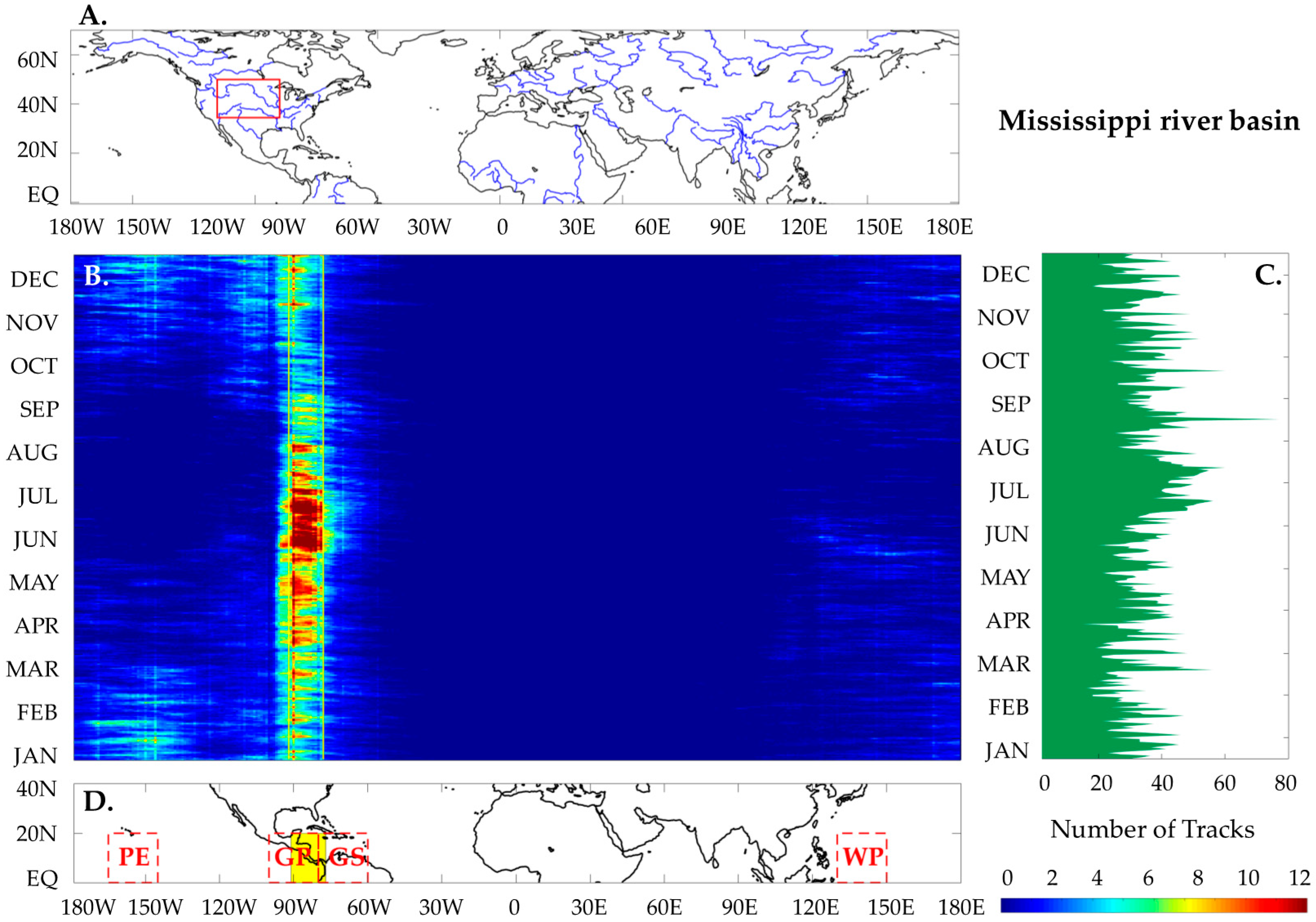
Figure 3.
Tropical moisture source identification for the Loire river basin. Plot (A) shows the study area in the red box, which is used to filter the TMEs tracks. Only those tracks entering the red box are retained to produce Plot (B). Plot (B) shows the calendar day average moisture tracks originating in the tropics [0–20° N] and entering the red box in Plot (A). The color scale reference bar for Plot (B) is on the bottom right. The band between the yellow lines in Plot (B) is defined by finding the yellow lines that the average annual total number of tracks starts to exceed the 80th percentile. Plot (C) shows the calendar day maximum and minimum numbers of tracks over the entire data period, originating within the region banded by the yellow lines in Plot (B). Plot (D) shows the four global TMEs source hotspots (‘PE,’ ‘GP,’ ‘GS’ and ‘WP’). The identified major TMEs source for the Loire is highlighted by the yellow box in Plot (D), corresponding to the banded area in Plot (B). Units of Plot (B) and Plot (C): number of tracks.
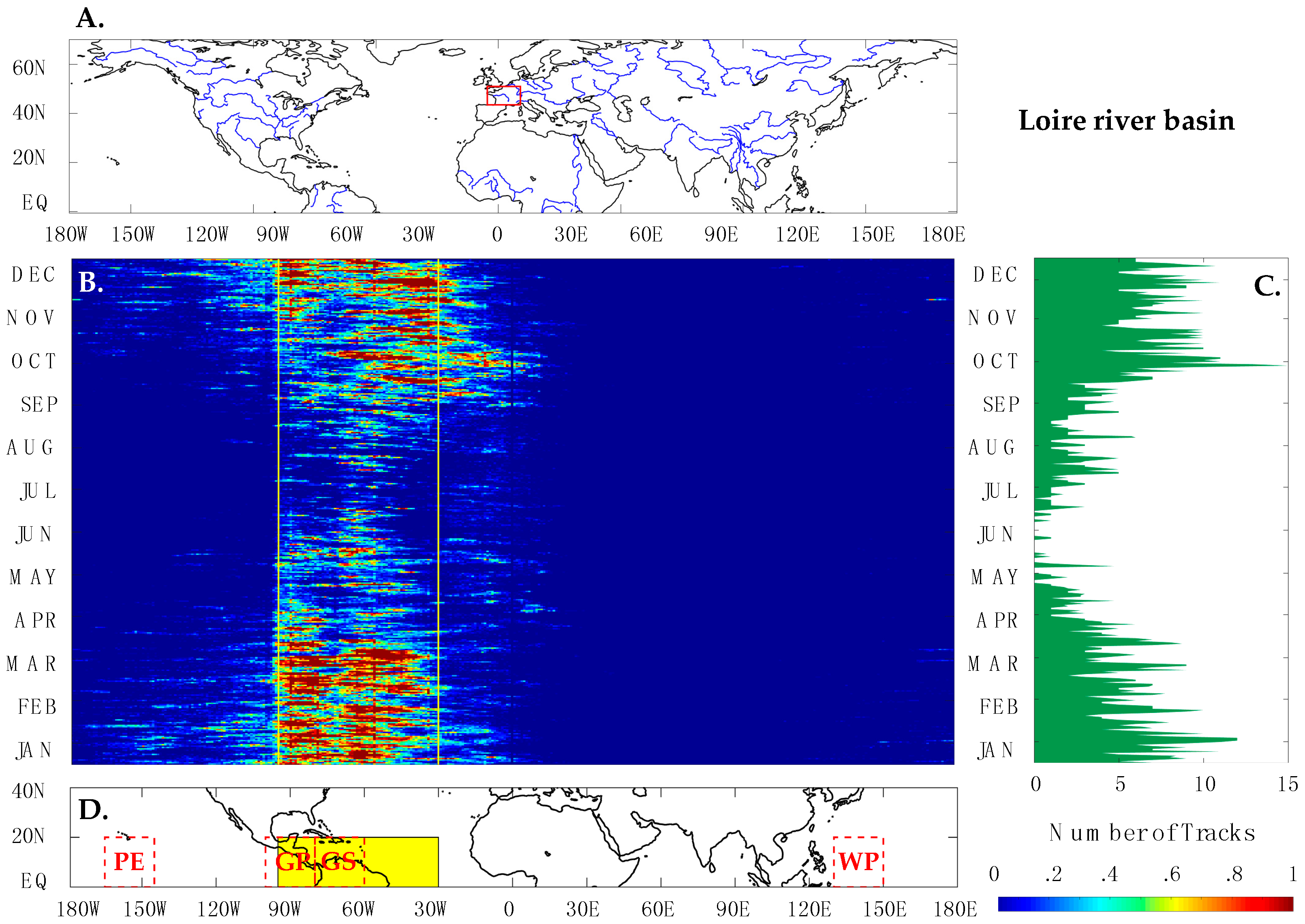
Figure 4.
Trajectory clustering for the three case study basins (red box with solid lines): (A) the Yangtze; (B) the Mississippi and (C) the Loire. Colored lines are the average trajectories for different clusters. The bars perpendicular to the trajectory lines cover 95% of the tracks belonging to that cluster. The yellow regions are the identified major TMEs source regions. The global hotspots of TMEs moisture sources are highlighted by the boxes with dashed red lines.


Figure 5.
Contributing number of TMEs tracks and the associated moisture release from each cluster for the Yangtze river basin. (A) the colors of the circles are consistent with the clusters in Figure 4. The center of the colored circle shows the total number of tracks (vertical axis) from the identified source to the basin for each year (bottom axis). The size of the circle represents the total amount of moisture release of those tracks. The size is proportional to (∑ΔQ)1.5. The scale reference of the circle is the panel on the right. The order of the clusters’ traveling speeds is given for fast reference to Figure 4B. (B) the colored lines show the smoothed time series of the annual contribution of each cluster in terms of moisture release. The contribution is calculated as the percentage of the total. The summary statistics of their contributions (mean, maximum and minimum values) are tabulated in the colored table. The colors of the clusters are consistent over the entire paper.

Figure 6.
Contributing number of TMEs tracks and the associated moisture release from each cluster for the Mississippi river basin. (A) the colors of the circles are consistent with the clusters in Figure 4. The center of the colored circle shows the total number of tracks (vertical axis) from the identified source to the basin for each year (bottom axis). The size of the circle represents the total amount of moisture release of those tracks. The size is proportional to (∑ΔQ)1.5. The scale reference of the circle is the panel on the right. The order of the clusters’ traveling speeds is given for fast reference to Figure 4B. (B) the colored lines show the smoothed time series of the annual contribution of each cluster in terms of moisture release. The contribution is calculated as the percentage of the total. The summary statistics of their contributions (mean, maximum and minimum values) are tabulated in the colored table. The colors of the clusters are consistent over the entire paper.
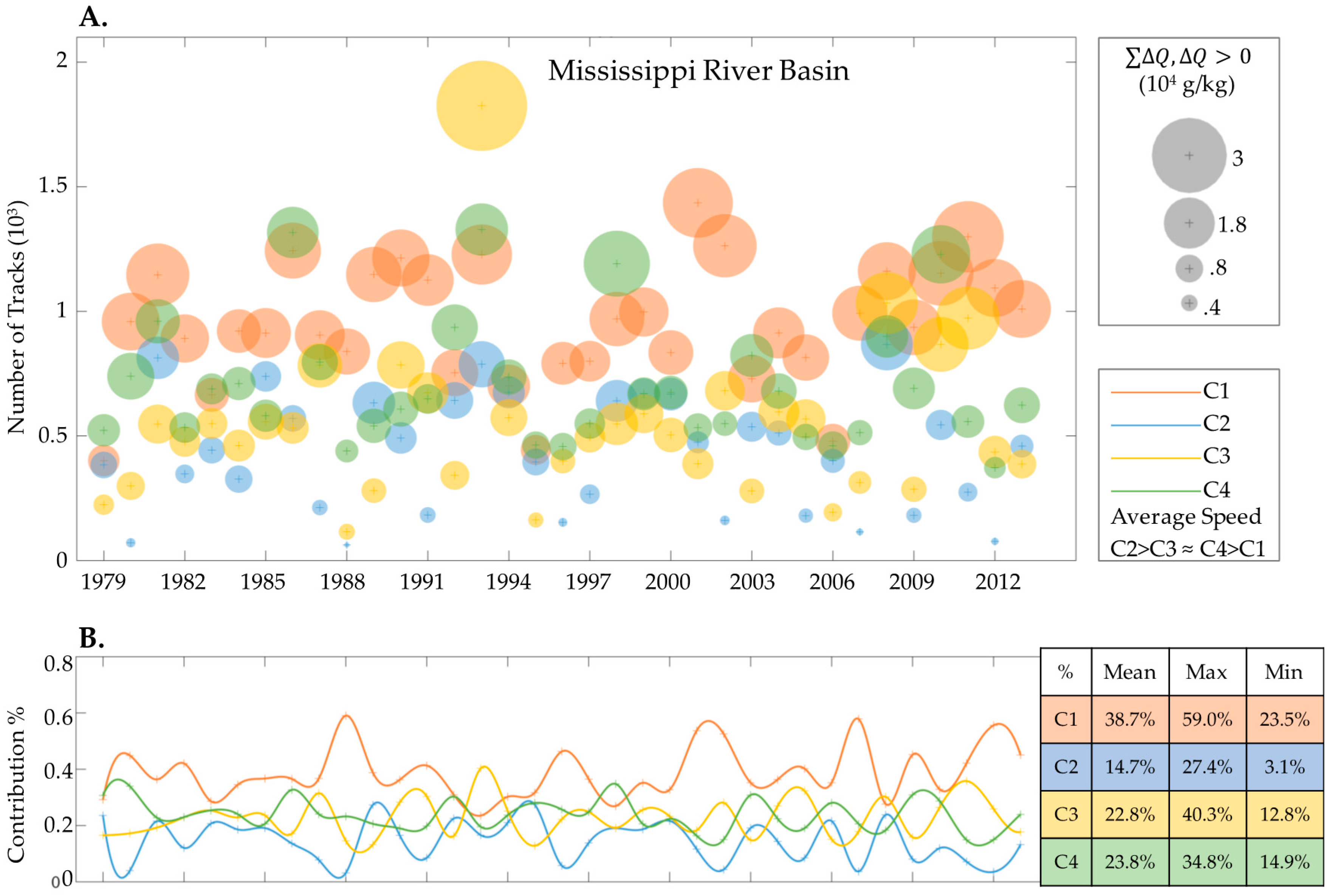
Figure 7.
Contributing number of TMEs tracks and the associated moisture release from each cluster for the Loire river basin. (A) the colors of the circles are consistent with the clusters in Figure 4. The center of the colored circle shows the total number of tracks (vertical axis) from the identified source to the basin for each year (bottom axis). The size of the circle represents the total amount of moisture release of those tracks. The size is proportional to (∑ΔQ). The scale reference of the circle is the panel on the right. The order of the clusters’ traveling speeds is given for fast reference to Figure 4B. (B) the colored lines show the smoothed time series of the annual contribution of each cluster in terms of moisture release. The contribution is calculated as the percentage of the total. The summary statistics of their contributions (mean, maximum and minimum values) are tabulated in the colored table. The colors of the clusters are consistent over the entire paper.
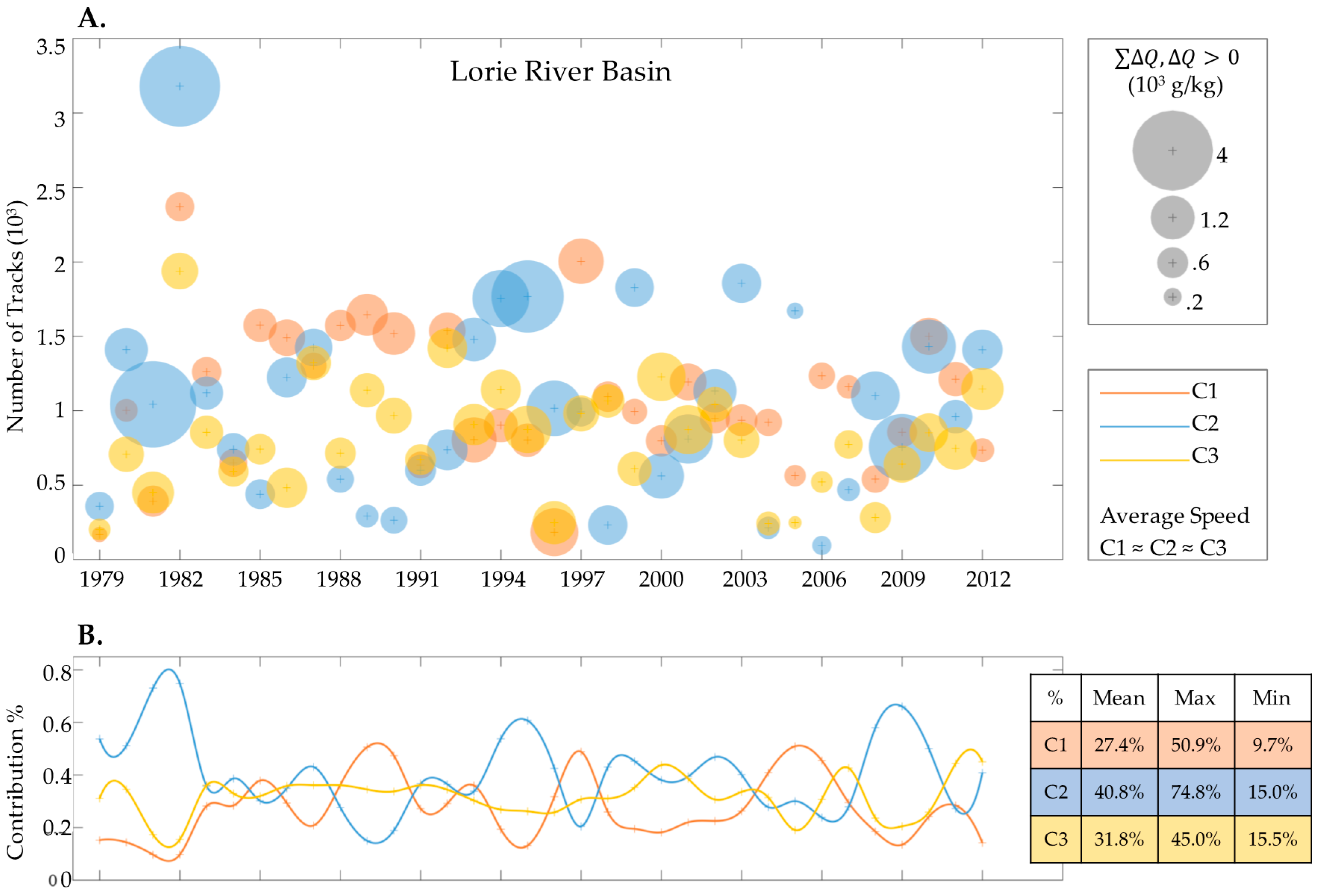
Figure 8.
The evolutions of the associated anomalous (1) atmospheric circulation and (2) moisture flux during the top 5% extreme precipitation periods using the 700 GHa and VIMFa composites for the Yangtze river basin from 7 days ahead (h) to the extreme precipitation days (a). The regions with statistical significant values at the 95% level are circled by the thick black lines.
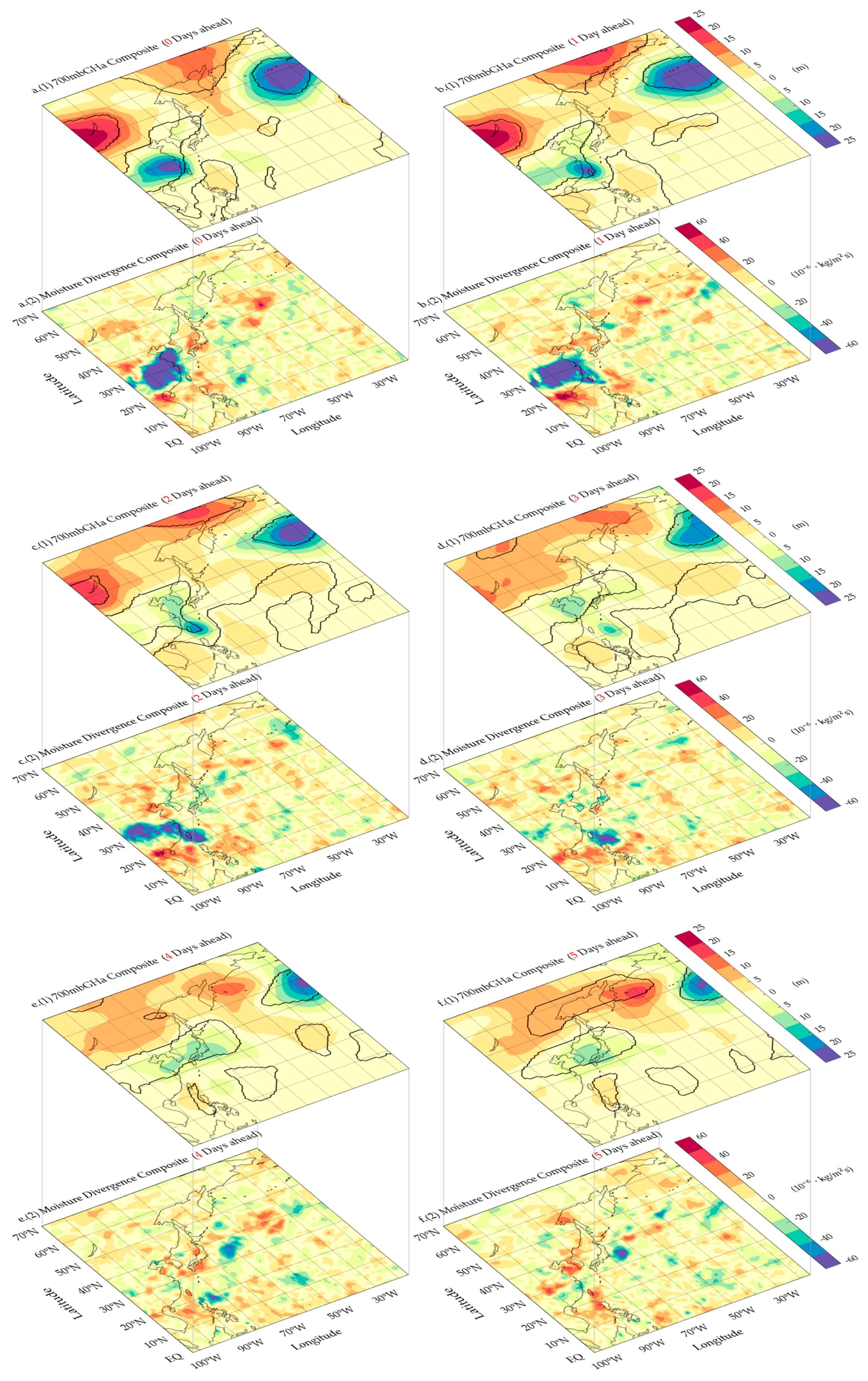

Figure 9.
The evolutions of the associated anomalous (1) atmospheric circulation and (2) moisture flux during the top 5% extreme precipitation periods using the 700 GHa and VIMFa composites for the Mississippi river basin from 7 days ahead (h) to the extreme precipitation days (a). The regions with statistical significant values at the 95% level are circled by the thick black lines.


Figure 10.
The evolutions of the associated anomalous (1) atmospheric circulation and (2) moisture flux during the top 5% extreme precipitation periods using the 700 GHa and VIMFa composites for the Loire river basin from 7 days ahead (h) to the extreme precipitation days (a). The regions with statistical significant values at the 95% level are circled by the thick black lines.


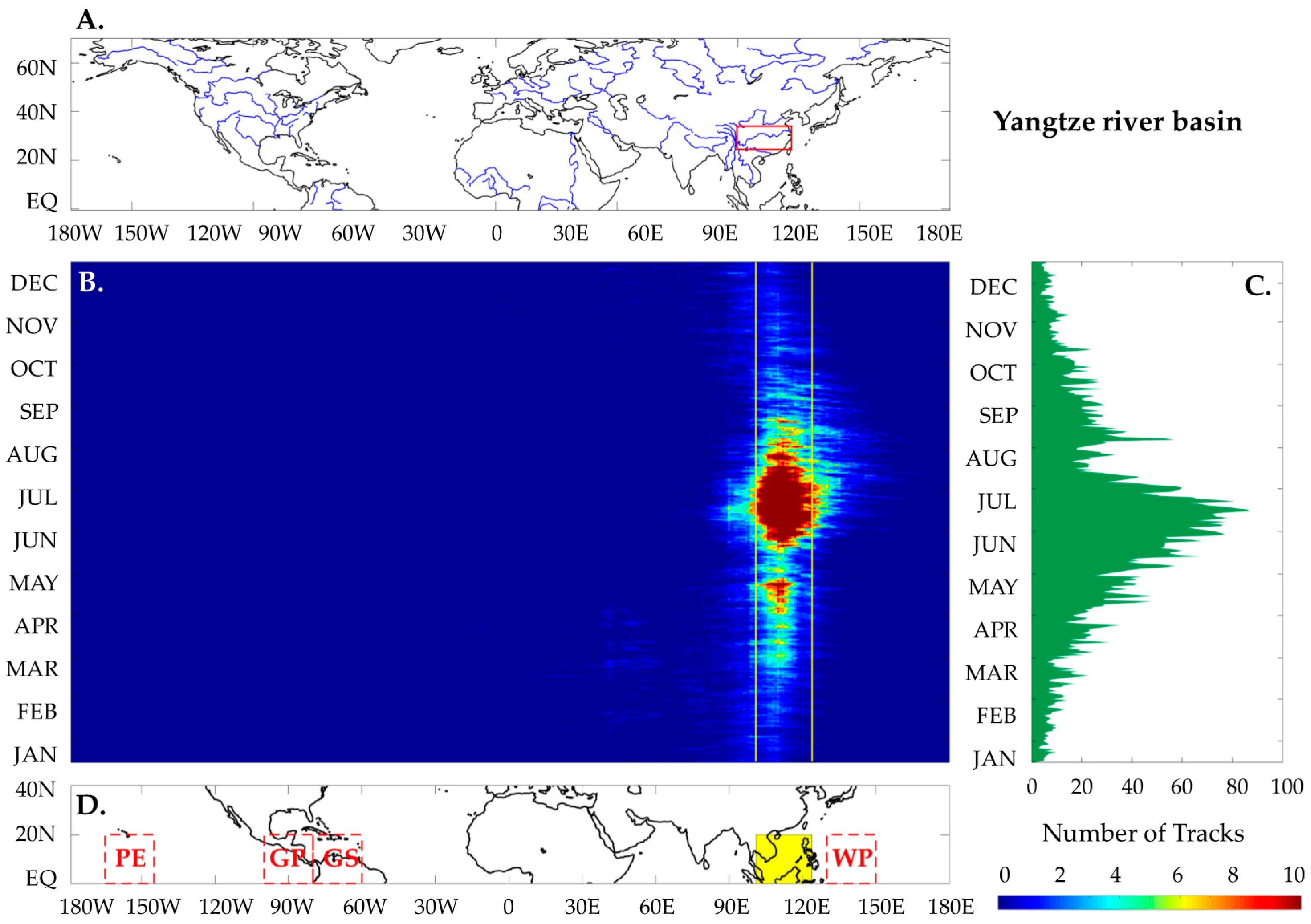
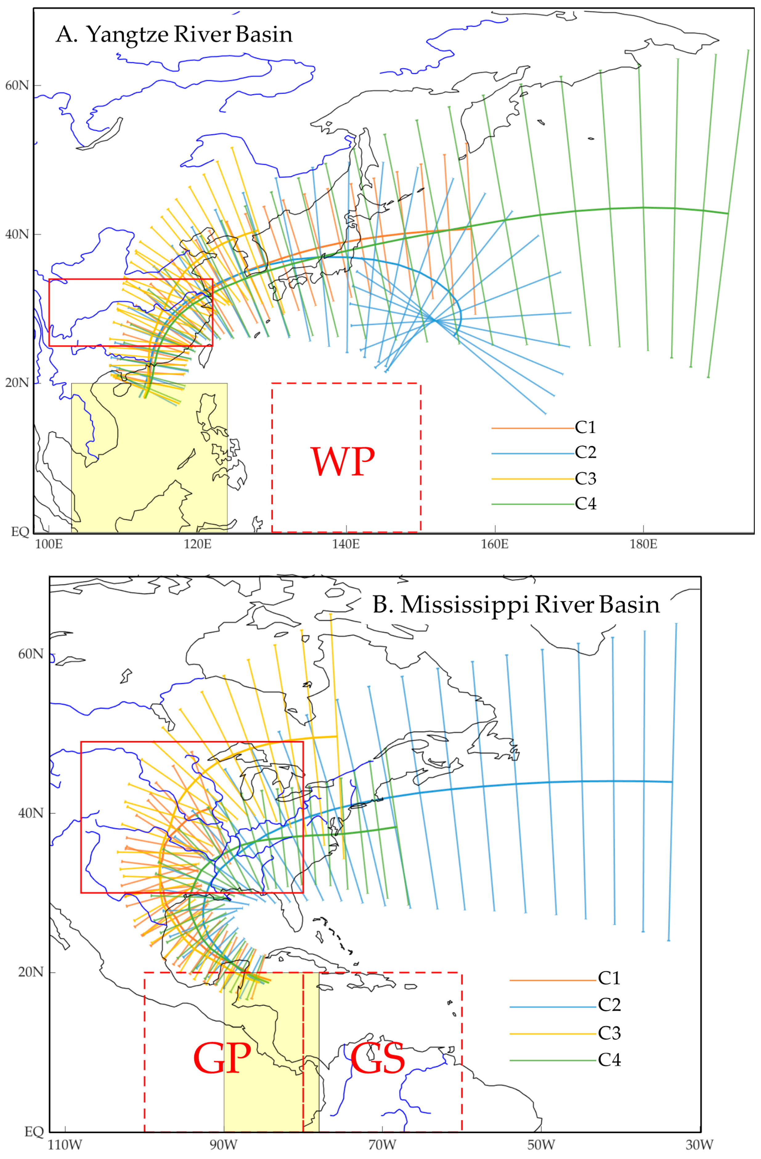
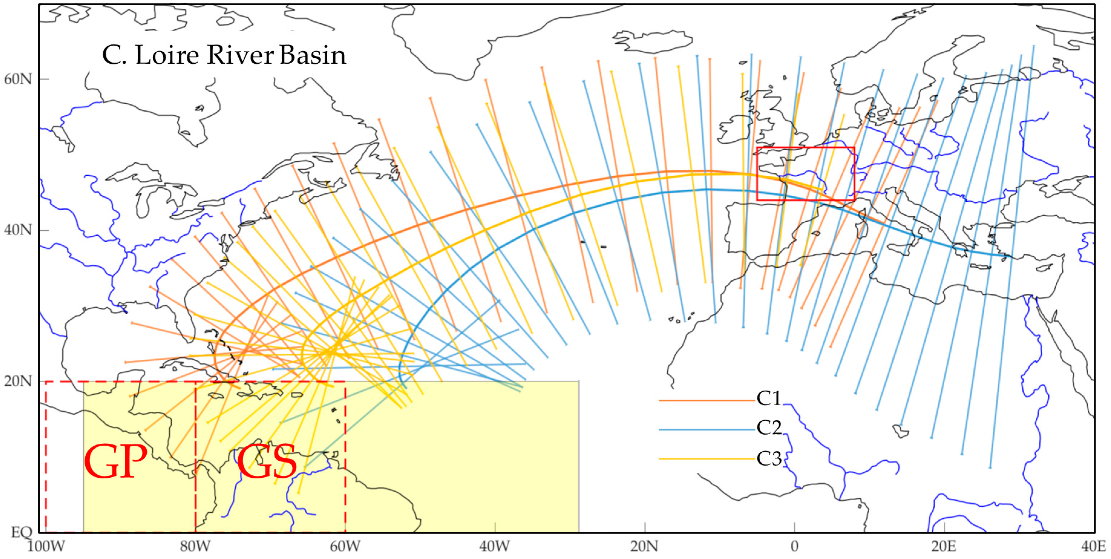
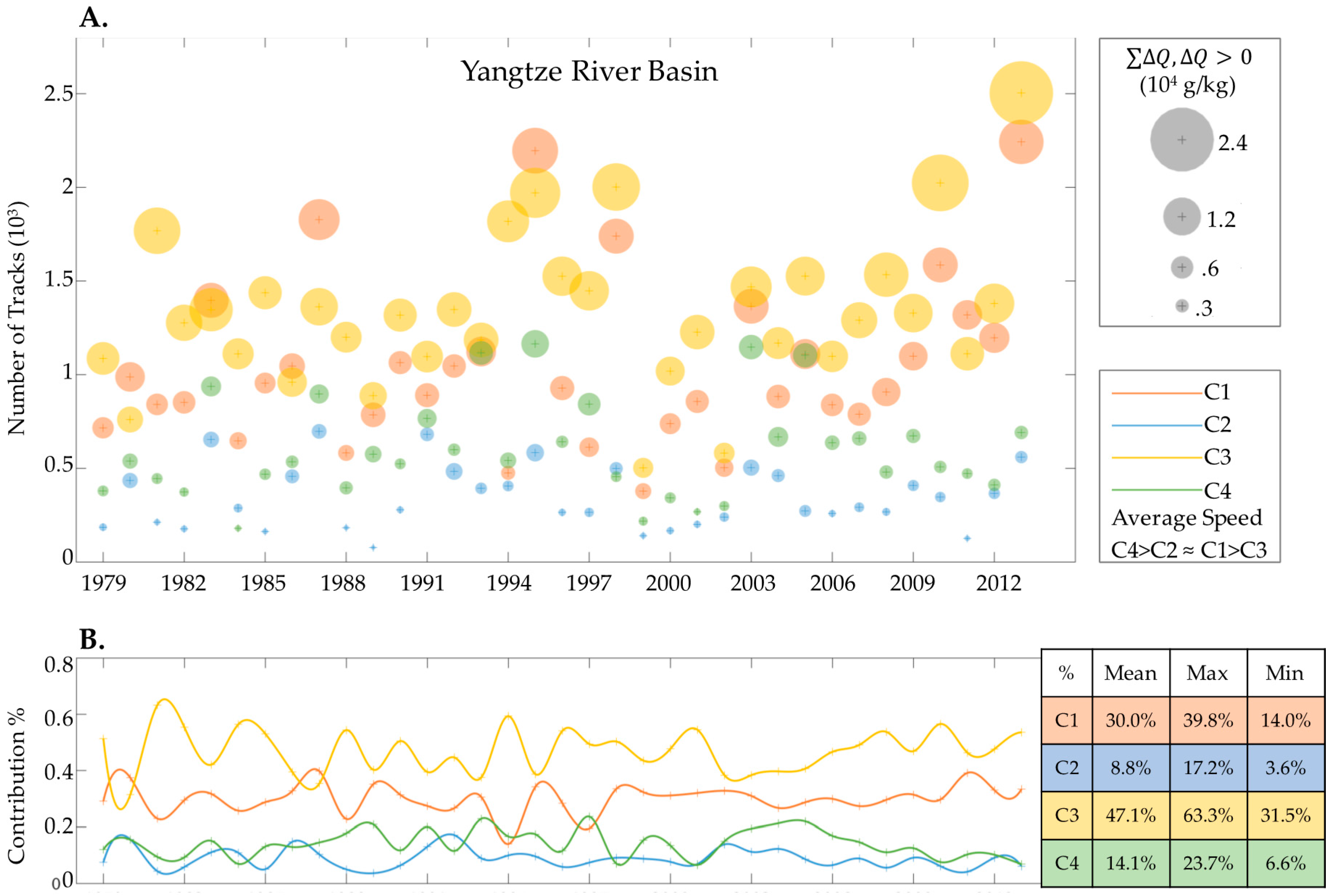
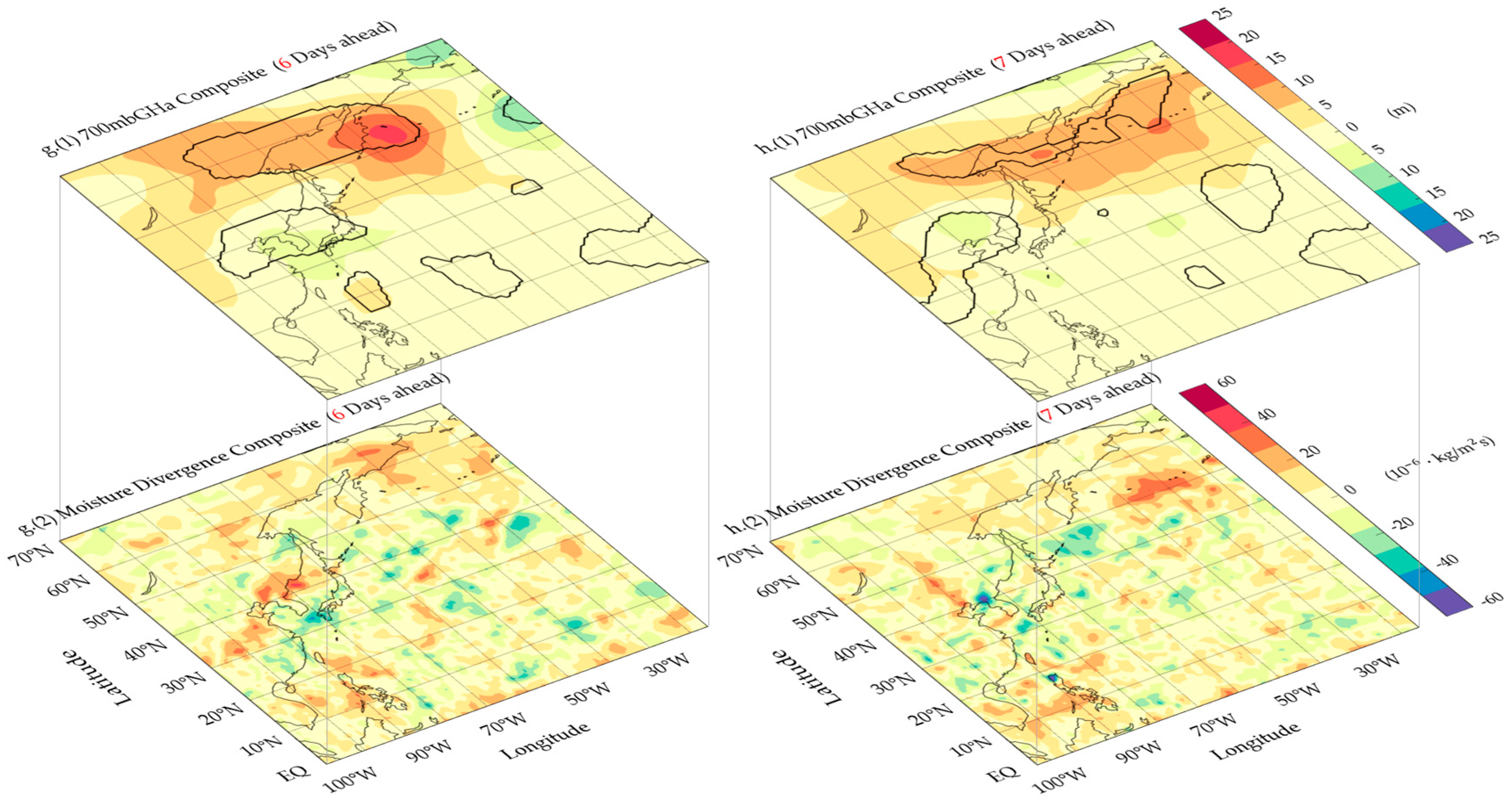
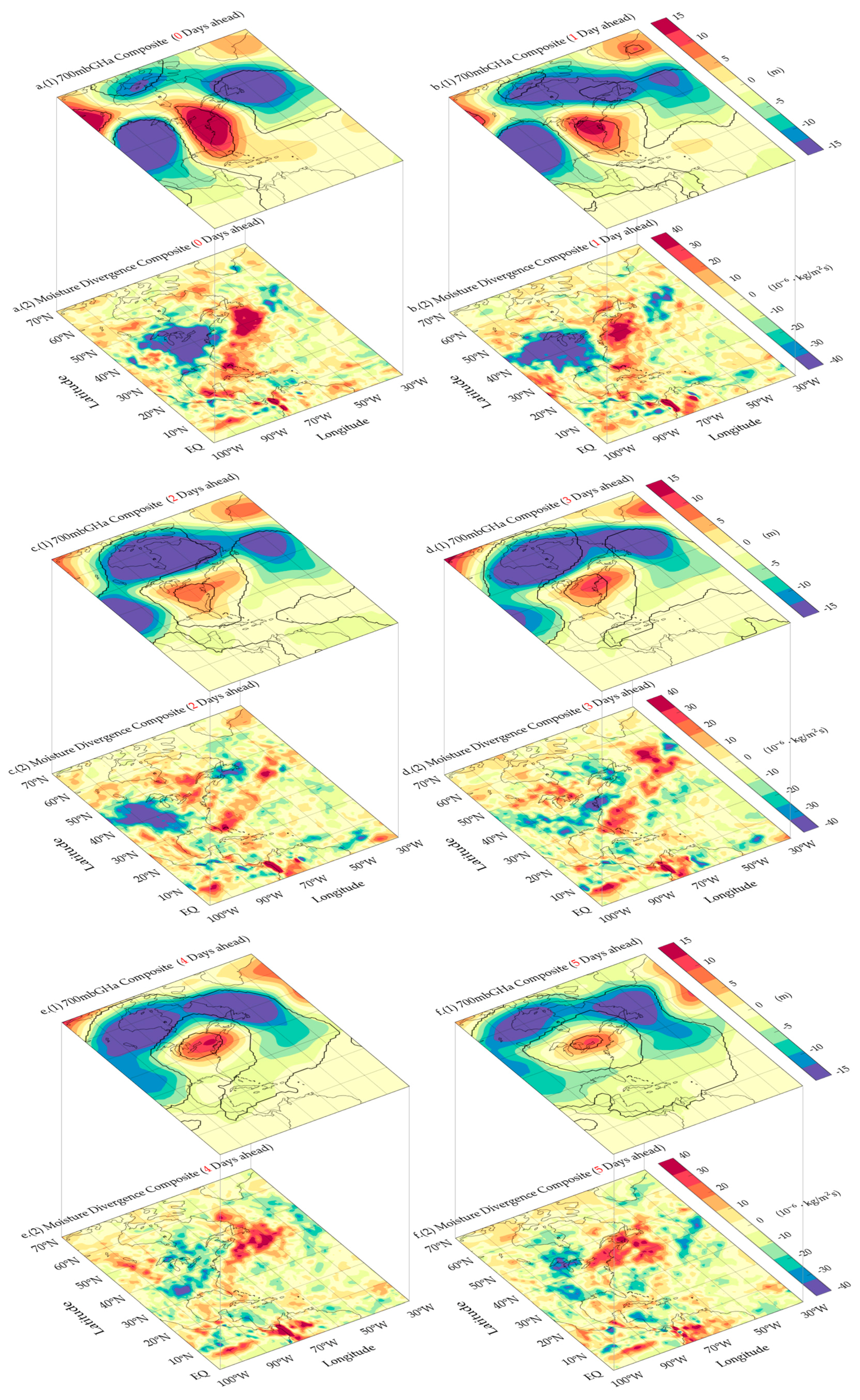
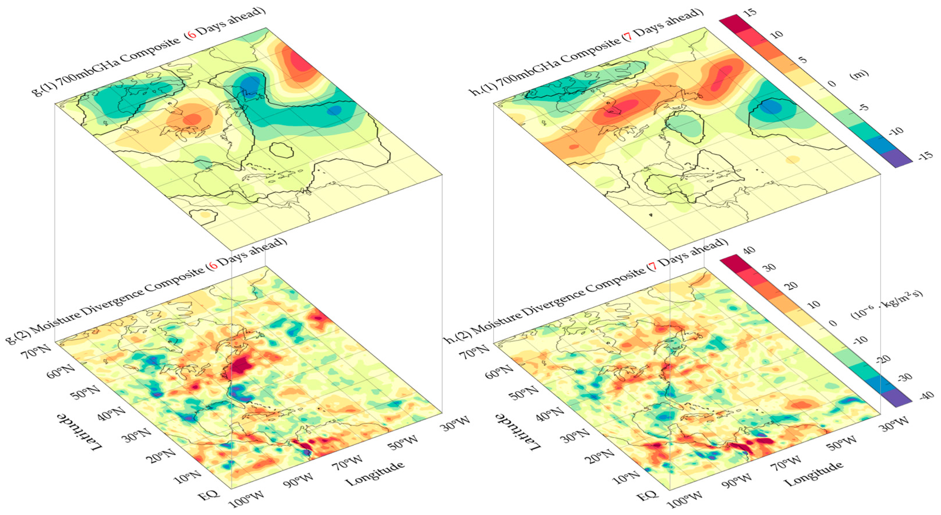
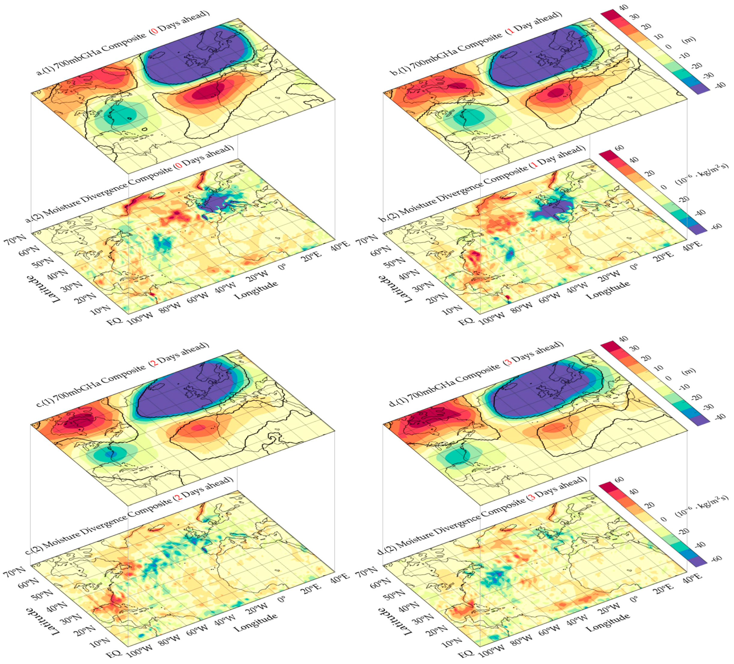
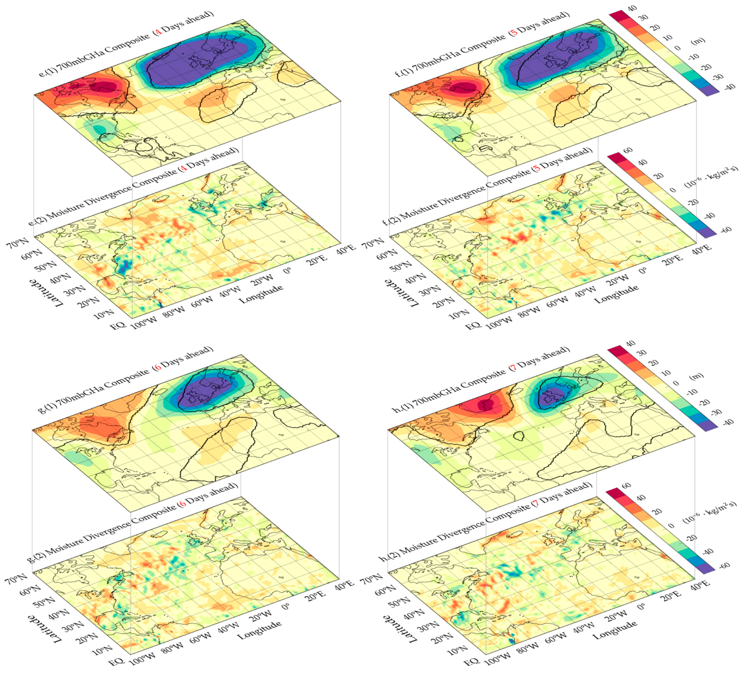
Table 1.
Summary of the case study locations, their main TMEs moisture source regions, the peak seasons and the resulting numbers of clusters from the analysis.
Table 1.
Summary of the case study locations, their main TMEs moisture source regions, the peak seasons and the resulting numbers of clusters from the analysis.
| River | Area Boundary | Main Source Region | Peak Season | Cluster # |
|---|---|---|---|---|
| Yangtze | [25–34° N, 100° E–122° E] | [0–20° N, 103° E–124° E] | Jul.–Aug. | 4 |
| Mississippi | [30–49° N, 108° W–80° W] | [0–20° N, 90° W–78° W] | Jun.–Jul. | 4 |
| Loire | [44–51° N, 5° W–8° E] | [0–20° N, 93° W–30° W] | Dec.–Jan. | 3 |
© 2017 by the authors. Licensee MDPI, Basel, Switzerland. This article is an open access article distributed under the terms and conditions of the Creative Commons Attribution (CC BY) license (http://creativecommons.org/licenses/by/4.0/).
Share and Cite
MDPI and ACS Style
Lu, M.; Hao, X. Diagnosis of the Tropical Moisture Exports to the Mid-Latitudes and the Role of Atmospheric Steering in the Extreme Precipitation. Atmosphere 2017, 8, 256. https://doi.org/10.3390/atmos8120256
AMA Style
Lu M, Hao X. Diagnosis of the Tropical Moisture Exports to the Mid-Latitudes and the Role of Atmospheric Steering in the Extreme Precipitation. Atmosphere. 2017; 8(12):256. https://doi.org/10.3390/atmos8120256
Chicago/Turabian StyleLu, Mengqian, and Xiaotian Hao. 2017. "Diagnosis of the Tropical Moisture Exports to the Mid-Latitudes and the Role of Atmospheric Steering in the Extreme Precipitation" Atmosphere 8, no. 12: 256. https://doi.org/10.3390/atmos8120256
Note that from the first issue of 2016, this journal uses article numbers instead of page numbers. See further details here.