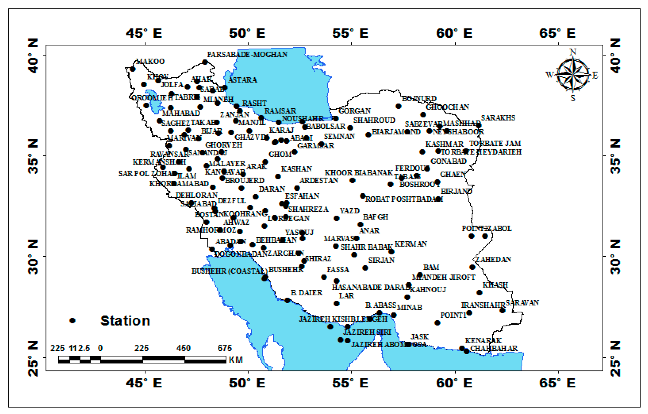
Figure 1.
Distribution of Stations.
Figure 1.
Distribution of Stations.
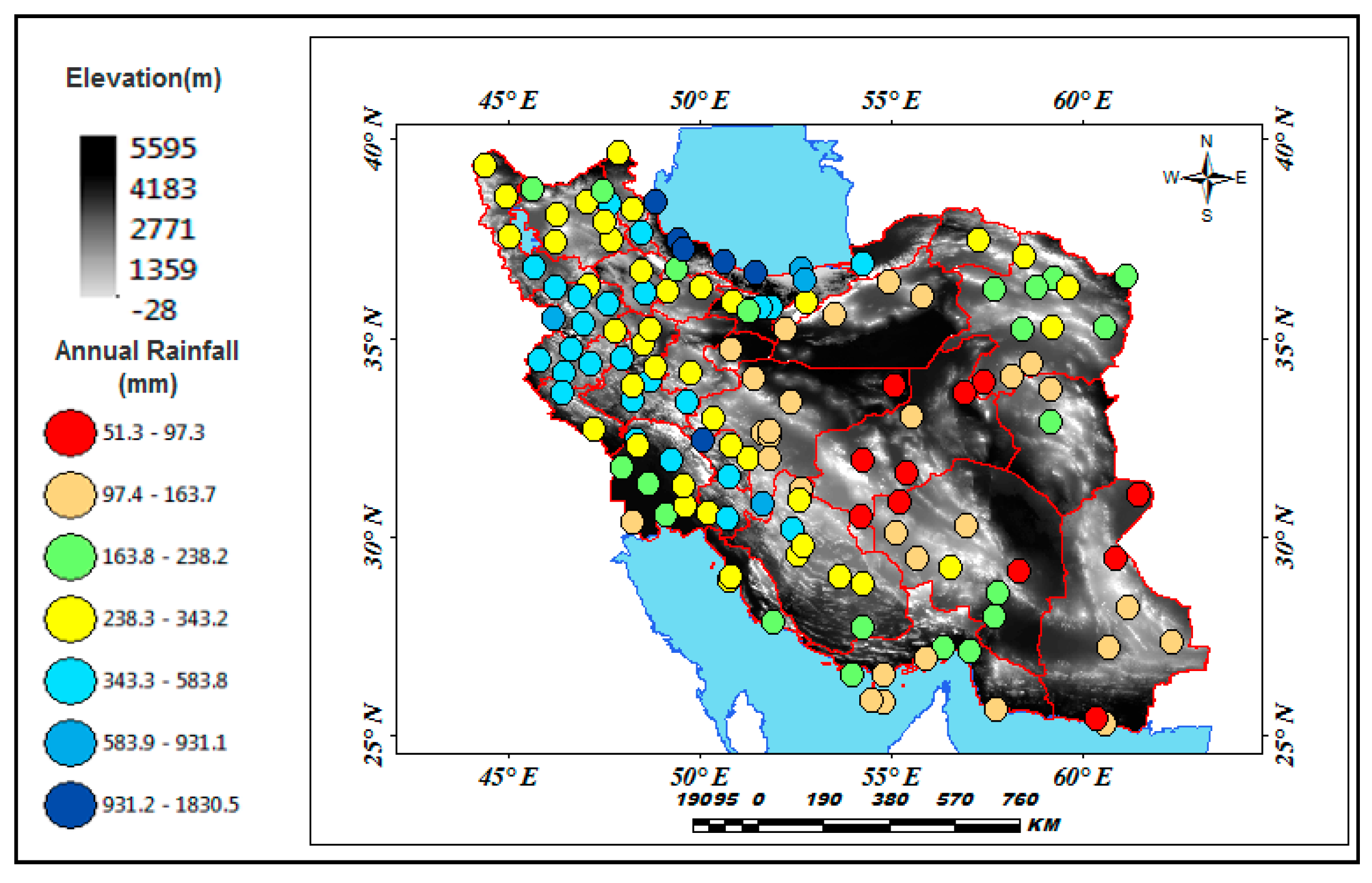
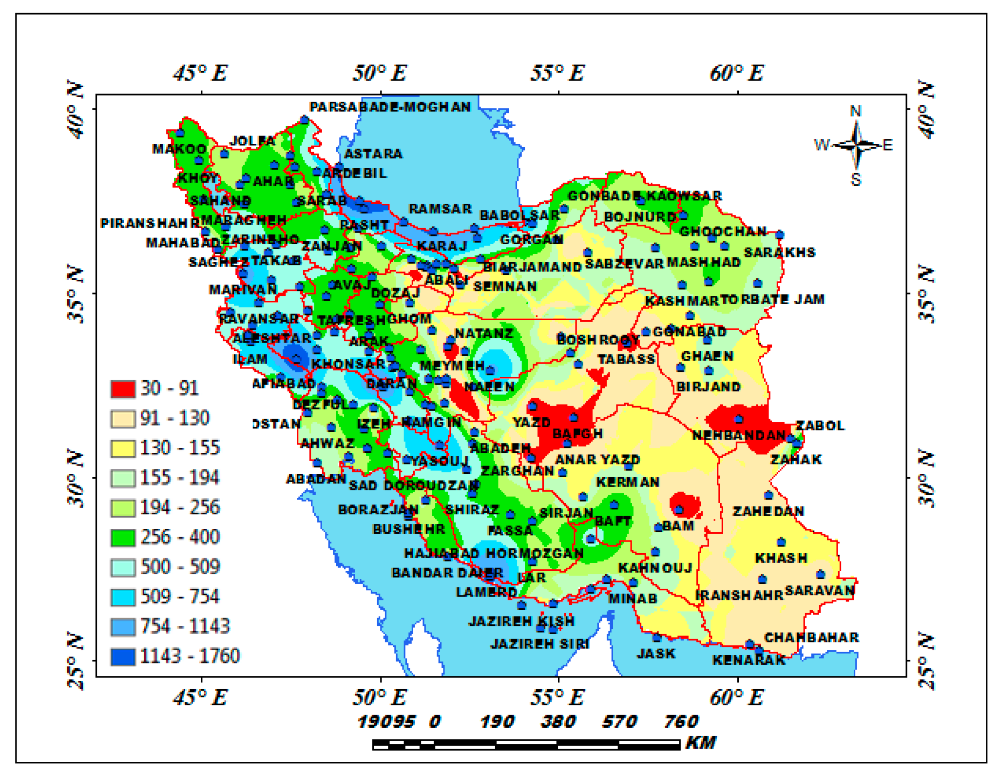
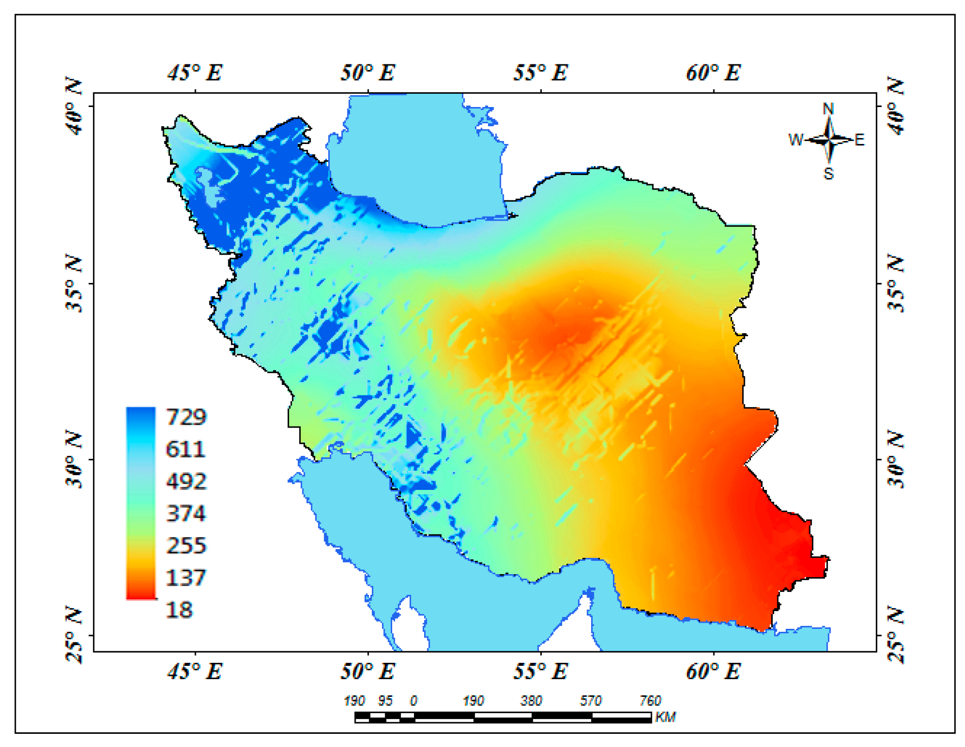
Figure 2.
DEM and rainfall distribution in Iran.
Figure 2.
DEM and rainfall distribution in Iran.
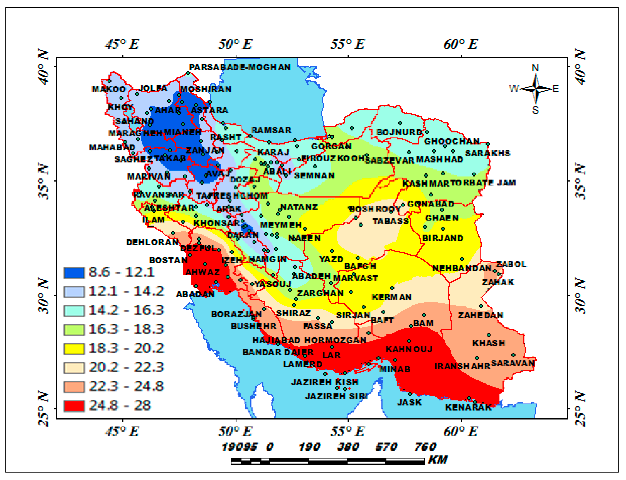
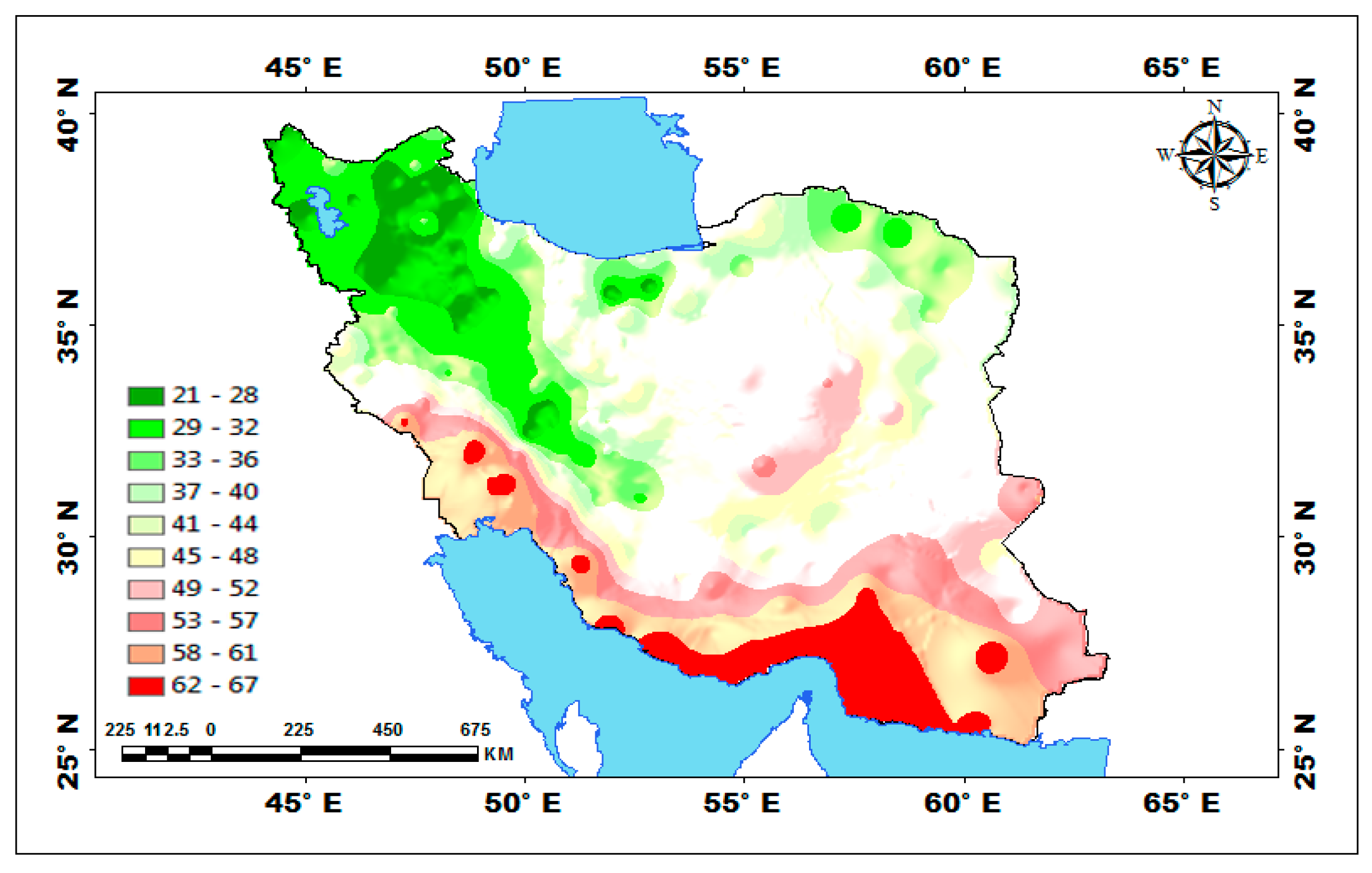
Figure 3.
Distribution of annual temperature.
Figure 3.
Distribution of annual temperature.
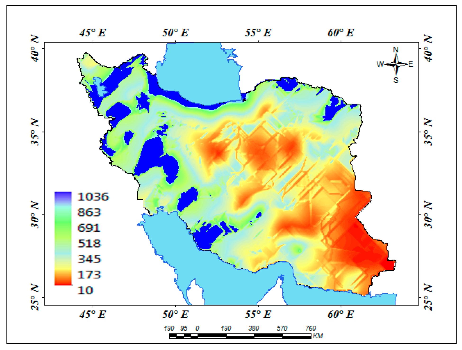
Figure 4.
Distribution of Annual Rainfall.
Figure 4.
Distribution of Annual Rainfall.
Figure 5.
The coefficient of variations of Annual Temperature (%).
Figure 5.
The coefficient of variations of Annual Temperature (%).
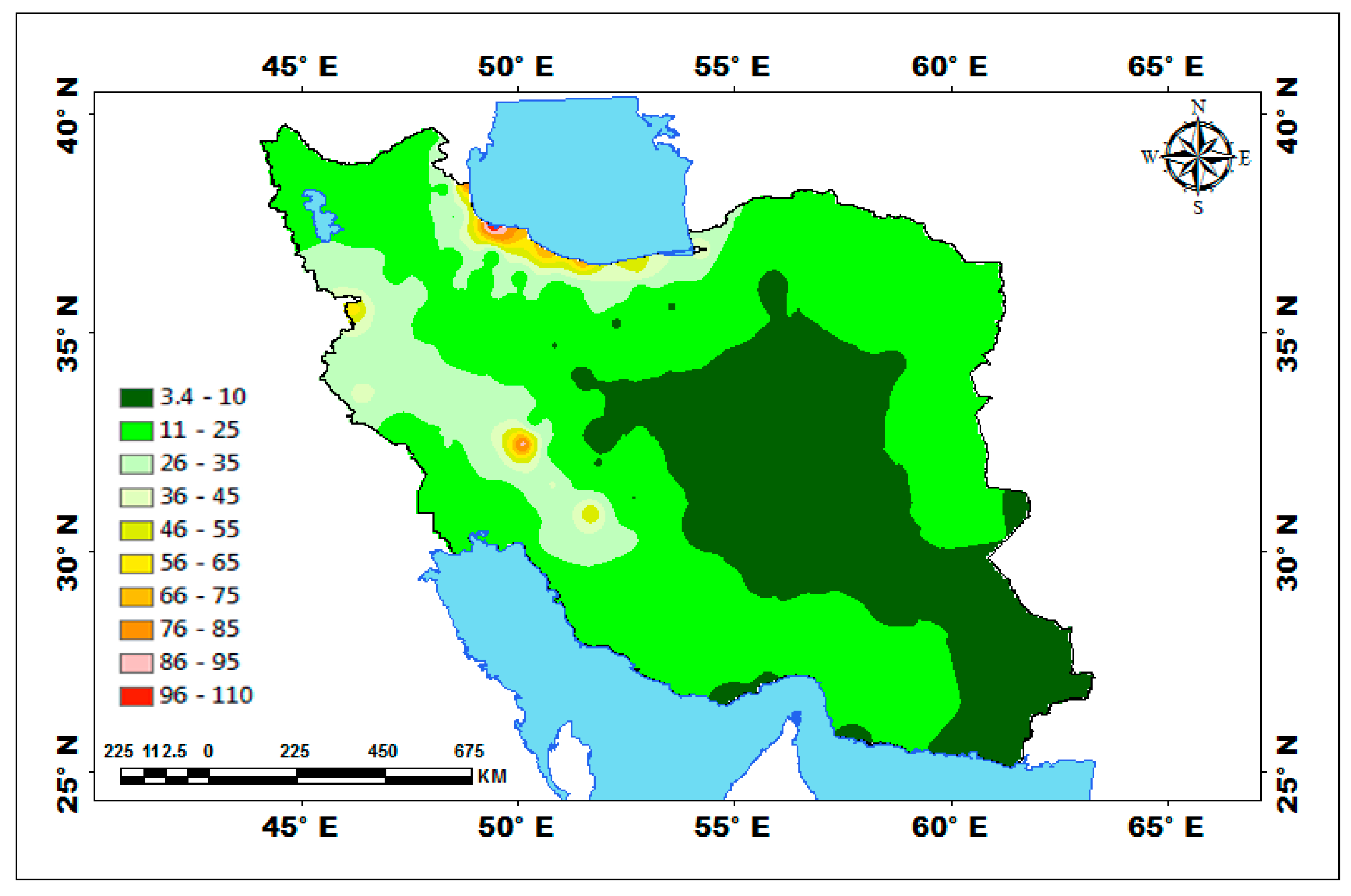
Figure 6.
The coefficient of variations of Annual Rainfall (%).
Figure 6.
The coefficient of variations of Annual Rainfall (%).
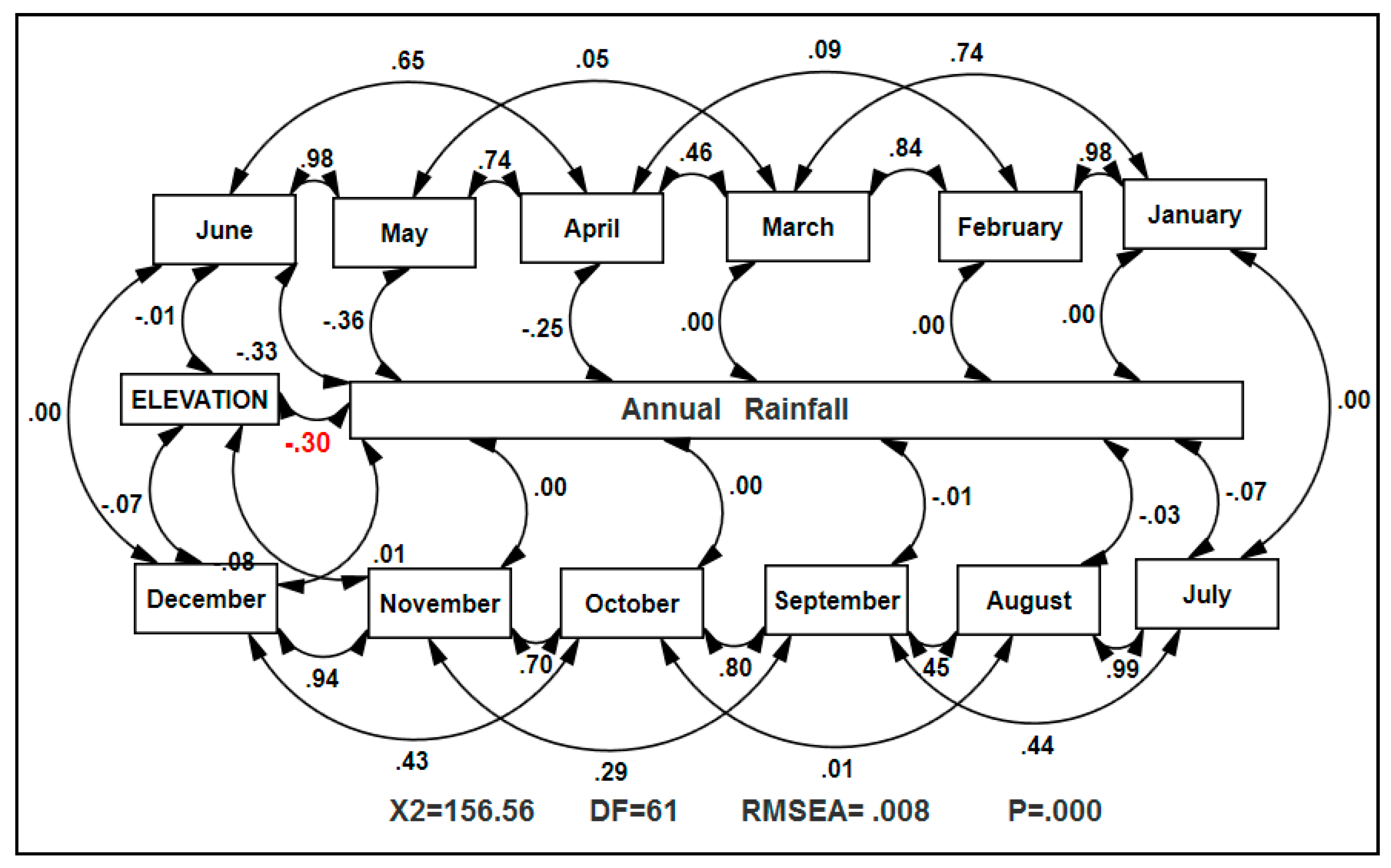
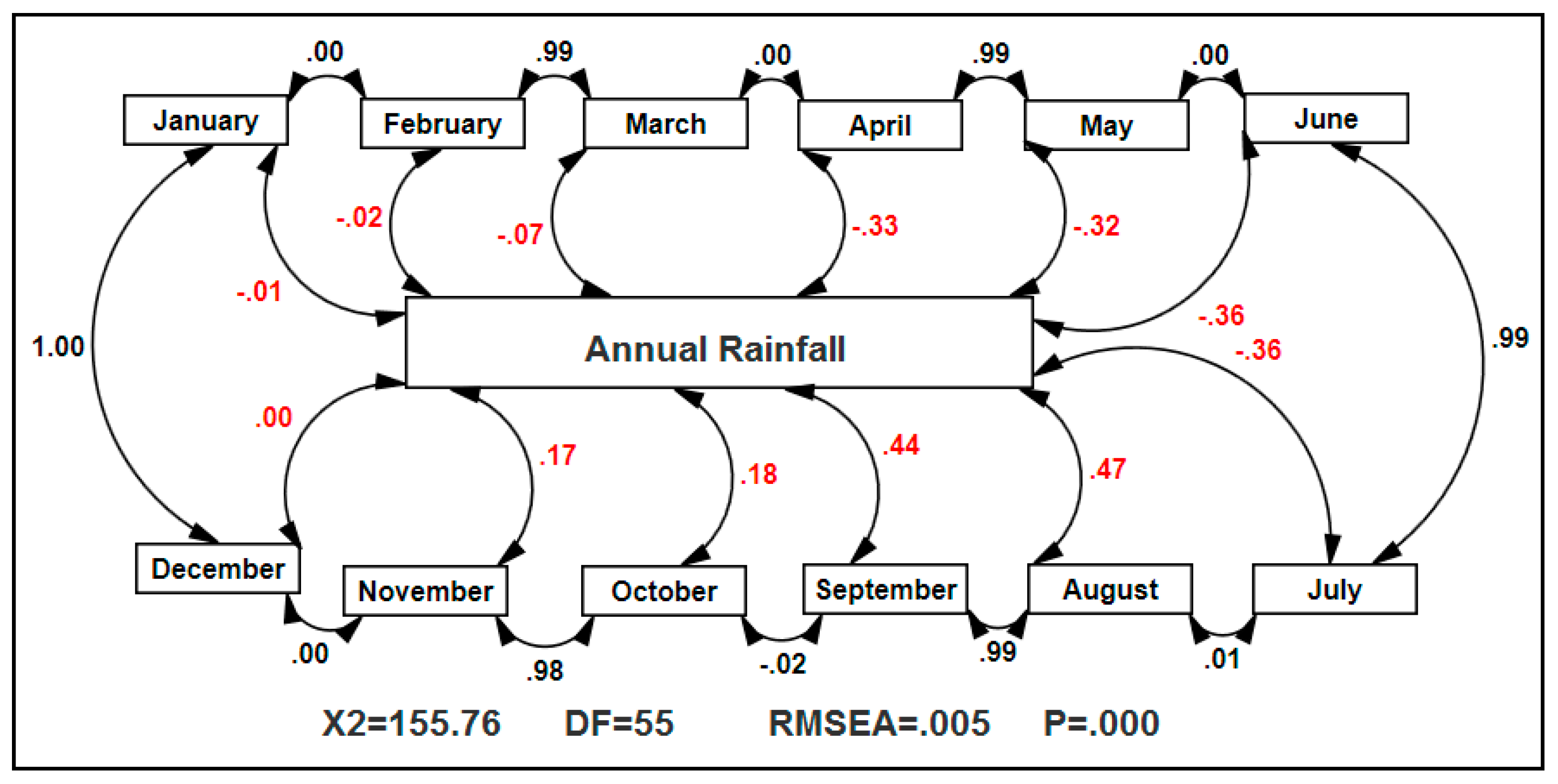
Figure 7.
The temporal correlation analysis between the monthly temperatures and annual rainfall. In
Figure 7, the double-headed arrows indicate covariance or correlation between pairs of variables. The correlation model shows that monthly temperatures have negative and positive correlations (red data) on annual rainfall. In the model summary presented in
Figure 7, we observed the overall chi-square (χ
2) value, together with its degrees of freedom, RMSEA 0.005 (a suitable fit) and probability value.
Figure 8.
The correlation between the monthly temperatures, elevation and annual rainfall.
Figure 8 also shows the temporal correlation coefficients between the temperatures, rainfall and elevation amounts for all stations.
Figure 8.
The correlation between the monthly temperatures, elevation and annual rainfall.
Figure 8 also shows the temporal correlation coefficients between the temperatures, rainfall and elevation amounts for all stations.
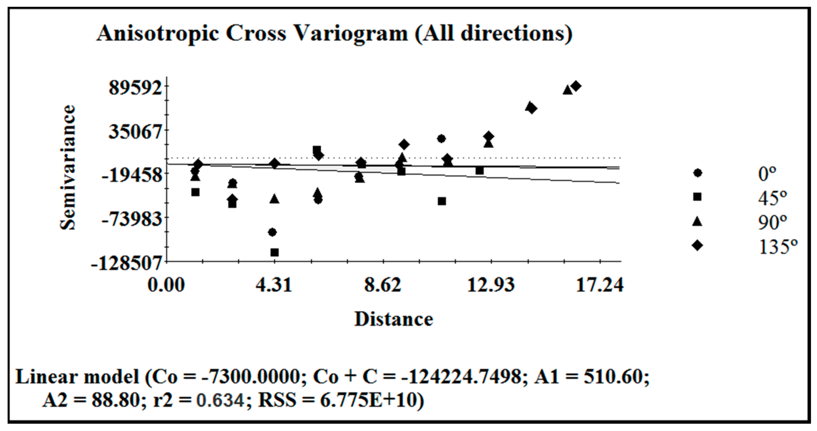
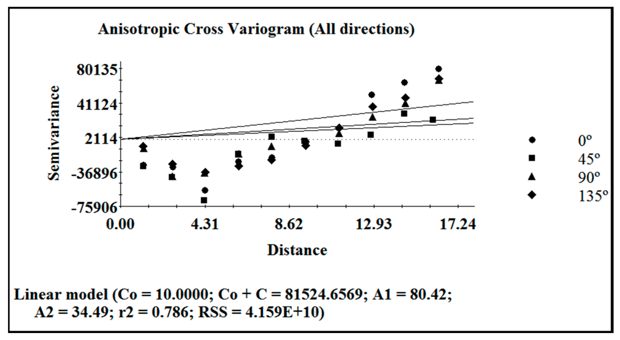
Figure 9.
Spatial correlation between the elevation and rainfall. Linear cross-variograms (dots) and measured spherical models (solid lines). The dashed lines show that there is a positive relationship between observed variables. Variogram factors: nugget variance or C0; Sill or C0 + C; Range or A (A1—the range parameter for the major axis of variation and A2—the range parameter for the minor axis); Ratio C/ (C0 + C) or RNS and RSS. The linear anisotropic model describes a straight-line variogram ( that γ (h) = semi variance for interval distance class h, h = lag interval, C0 = nugget variance ≥0, C = structural variance ≥ C0 , A1 = range parameter for the major axis (Ф) and A2 = range parameter for the minor axis (Ф + 90).
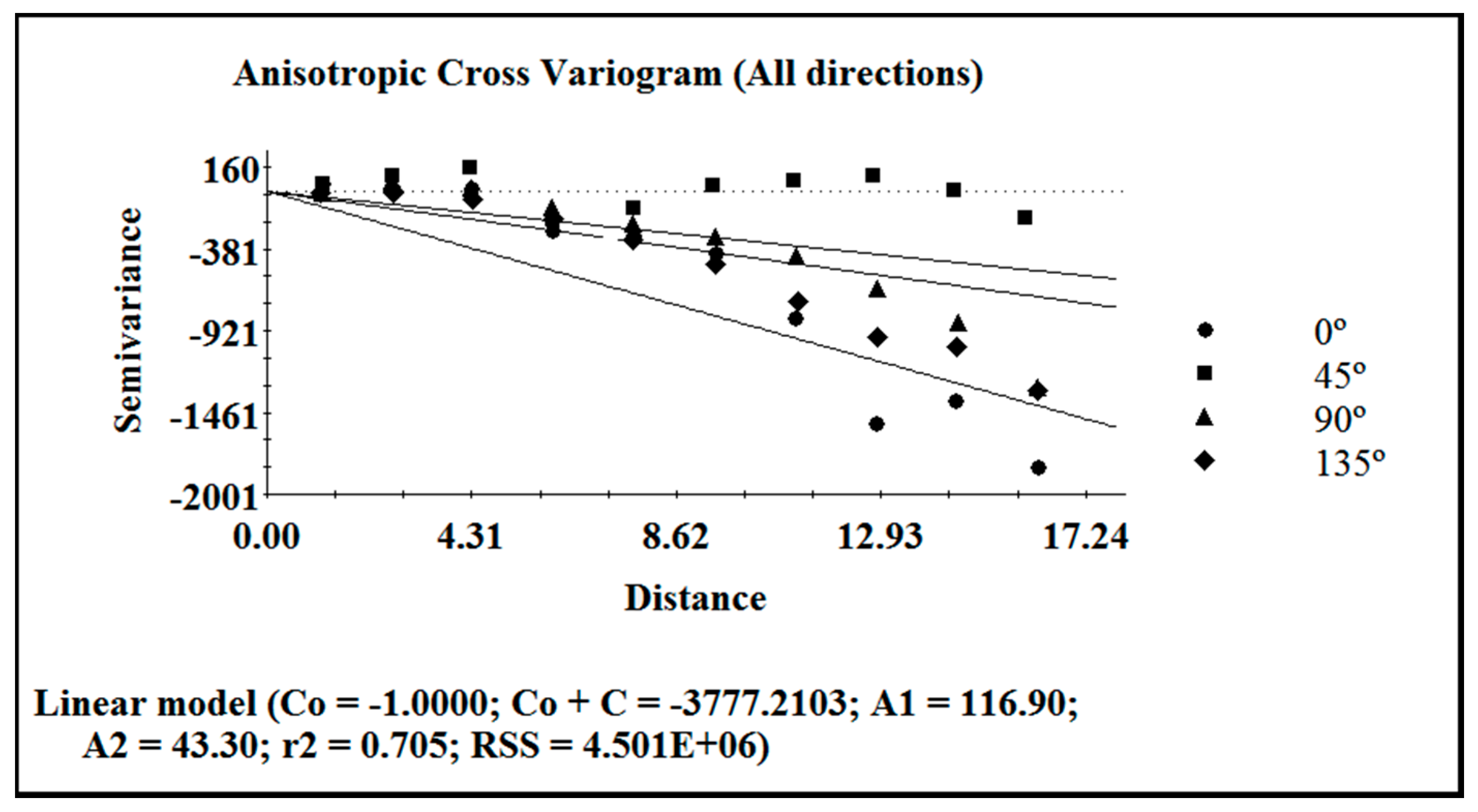
Figure 10.
Spatial correlation between the Temperature and Rainfall.
Figure 10.
Spatial correlation between the Temperature and Rainfall.
Figure 11.
Spatial correlation between the DEM and Rainfall.
Figure 11.
Spatial correlation between the DEM and Rainfall.
Figure 12.
The effectiveness analysis between the monthly temperatures and annual rainfall. Effectiveness model analyzed casually in each climatic series. The single-headed arrows denote causal relationships and the impact of one variable on another; the double-headed arrows indicate covariance or correlation between pairs of variables. The SEM model shows that monthly temperatures have a direct effect (red data) on annual rainfall. Monthly temperatures have direct effects (positive and negative) on annual rainfall and monthly temperatures have a correlation with neighborhood series. An error term (e1) is associated with an observed variable (annual rainfall). In the model summary presented in
Figure 12, the overall chi-square (χ
2) value, together with its degrees of freedom and probability value was observed.
Figure 13.
The effectiveness between the monthly temperatures and annual rainfall (first model). Monthly effectiveness investigated casually in rainfall series. The effectiveness model shows that eight monthly temperature series (January, April, May, June, July, October, November and September based on Standardized β higher) have an indirect effect on annual rainfall. Monthly temperature series (February, March, August and December) have direct effects (positive and negative) on annual rainfall.
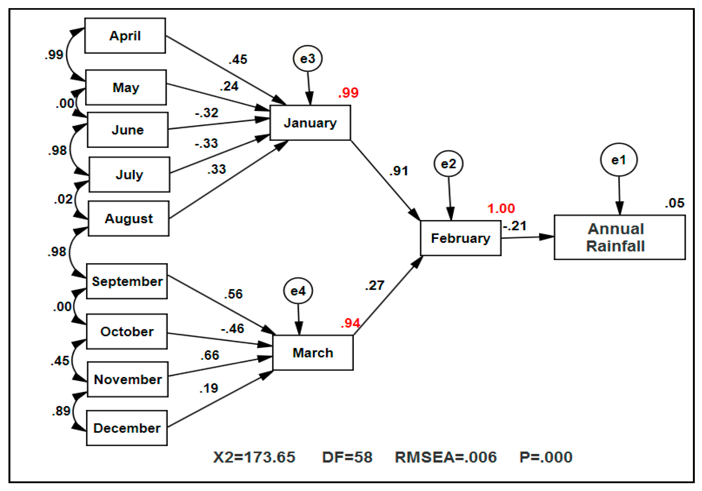
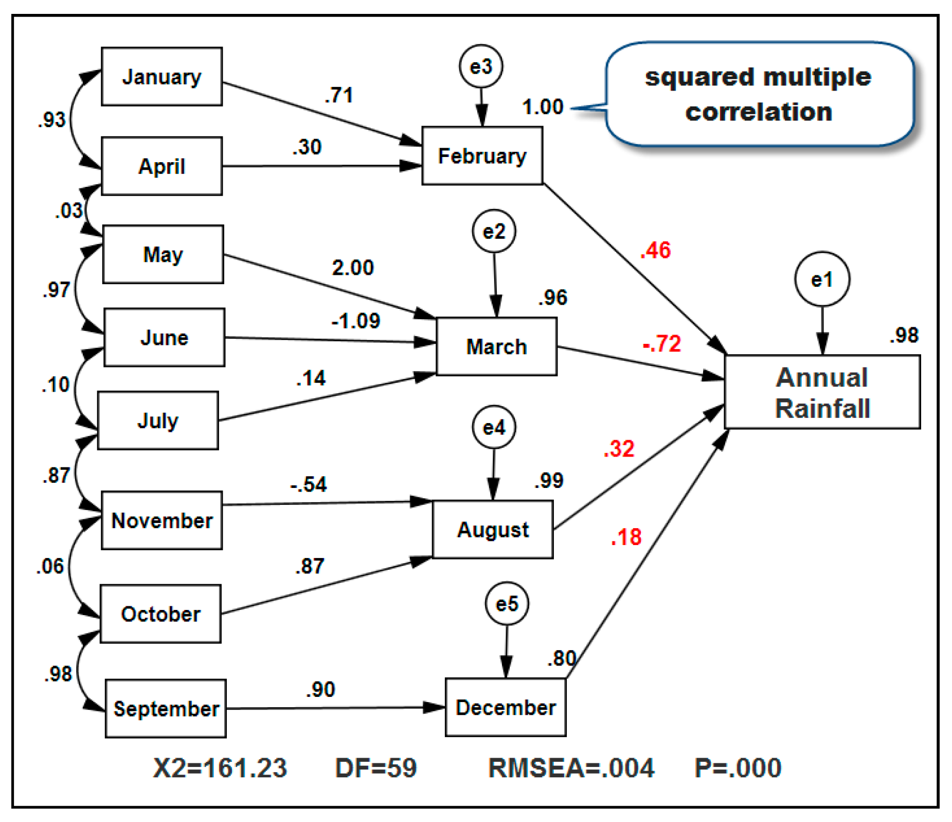
Figure 14.
The effectiveness between the monthly temperature and annual rainfall (second model). Monthly effectiveness investigated on annual rainfall series. The effectiveness model shows that nine monthly temperature series (January, March, April, May, June, July, August, September, October, November and December) have indirect effects on annual rainfall. February temperature has a direct effect (negative effect) on annual rainfall. According to
Figure 14, there is significant (0.94 < R
2 < 1) effectiveness (red data) between the temperature series and annual rainfall in Iran.
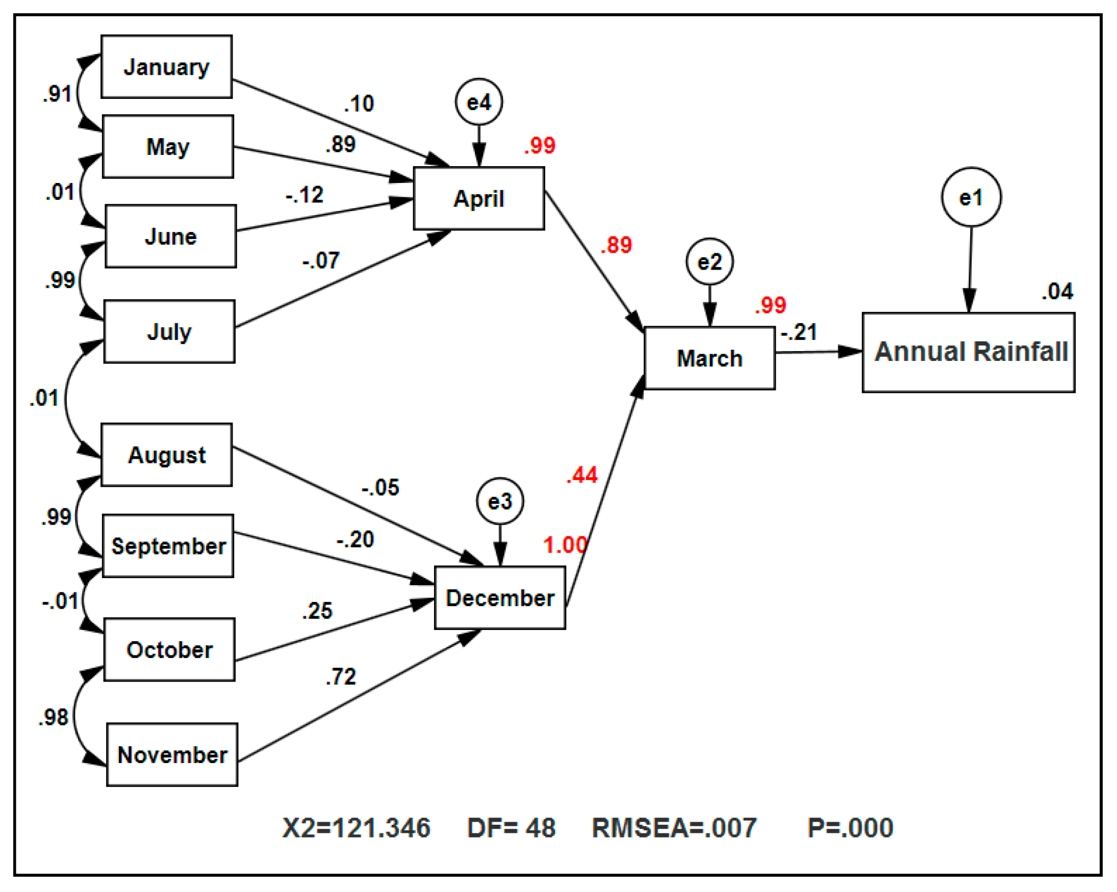
Figure 15.
The effectiveness between the monthly temperature and annual rainfall (third model). Monthly effectiveness investigated on annual rainfall series. The effectiveness model shows that ten monthly temperature series (January, April, May, June, July, August, September, October, November and December) have an indirect effect on annual rainfall. March temperature has a direct effect (negative effect) on annual rainfall.
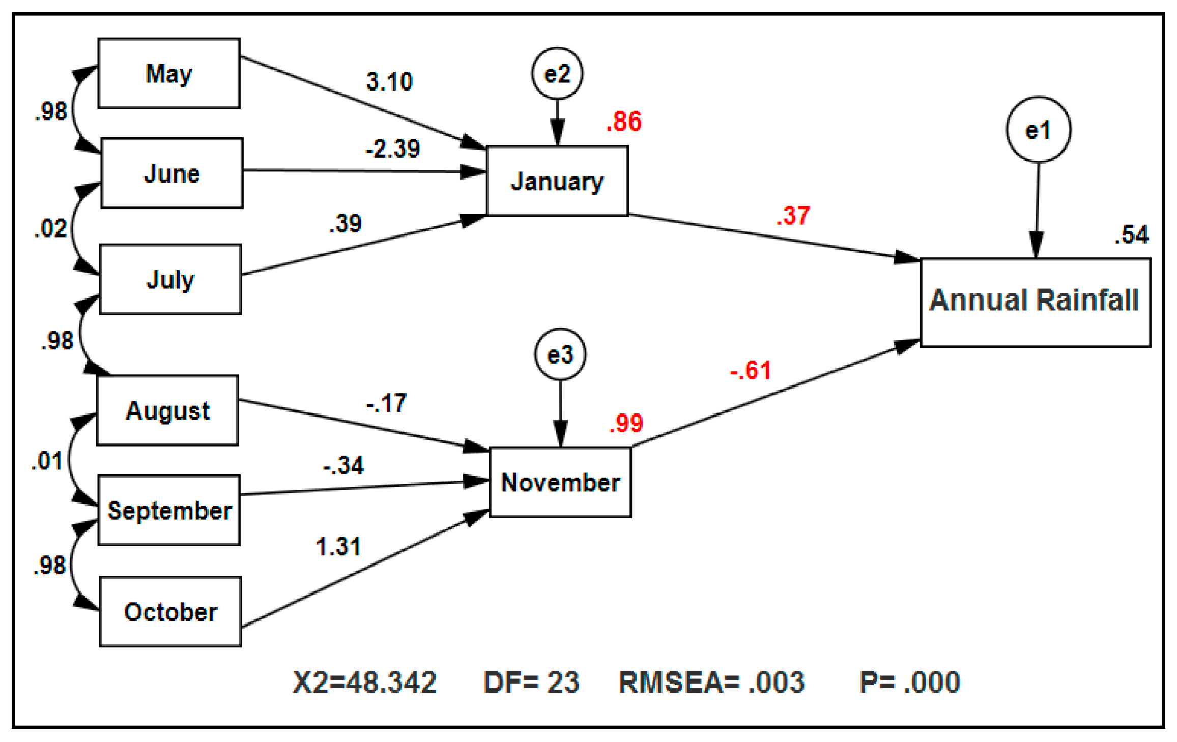
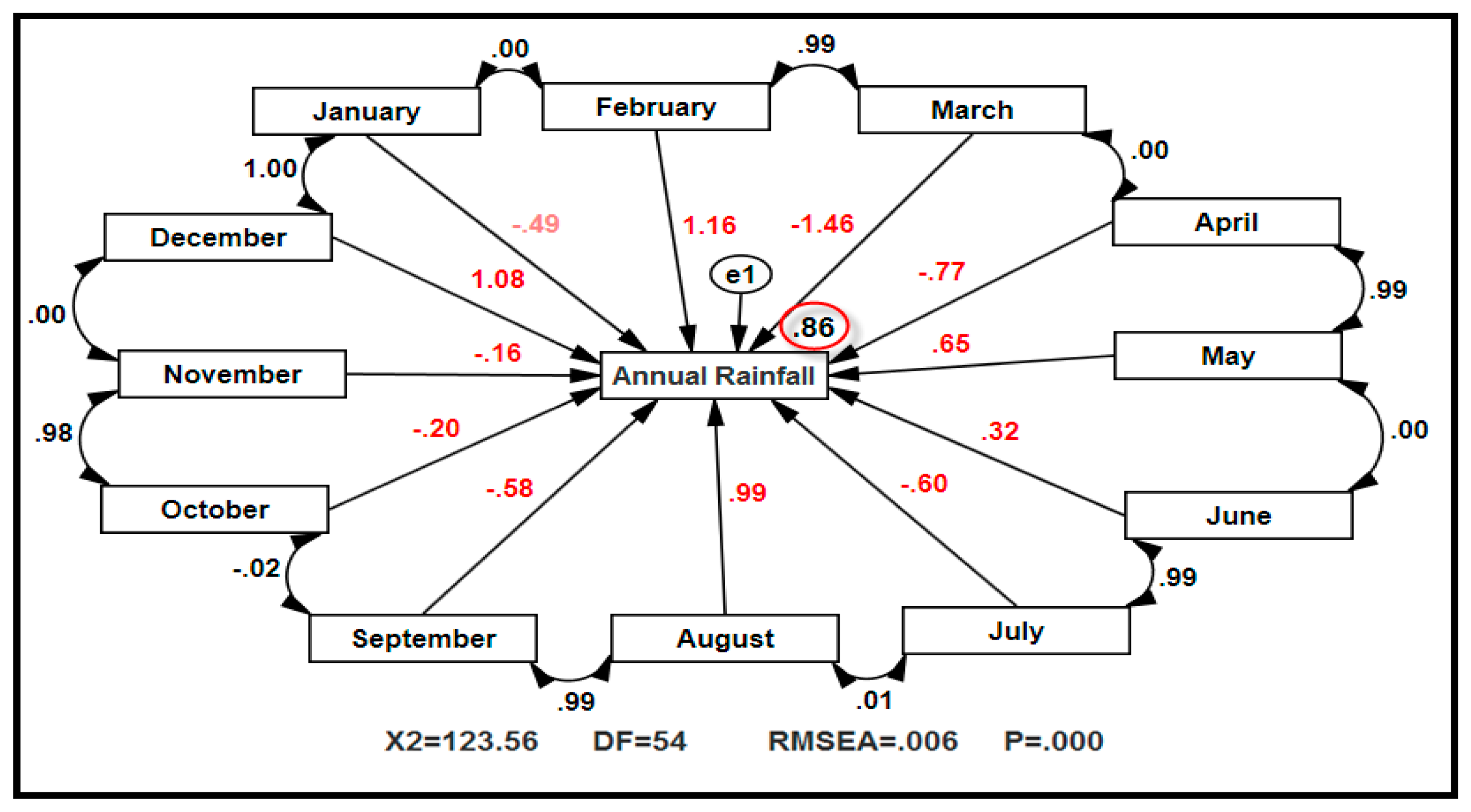
Figure 16.
The effectiveness between the monthly temperature and annual rainfall (fourth model). Monthly effectiveness investigated on annual rainfall series. The effectiveness model shows that eight monthly temperature series (May, June, July, August, September, October, November and December) have indirect effects on annual rainfall. January and November temperature series have a direct effect (negative and positive effects) on annual rainfall (0.86 < R2 < 0.99, red data).
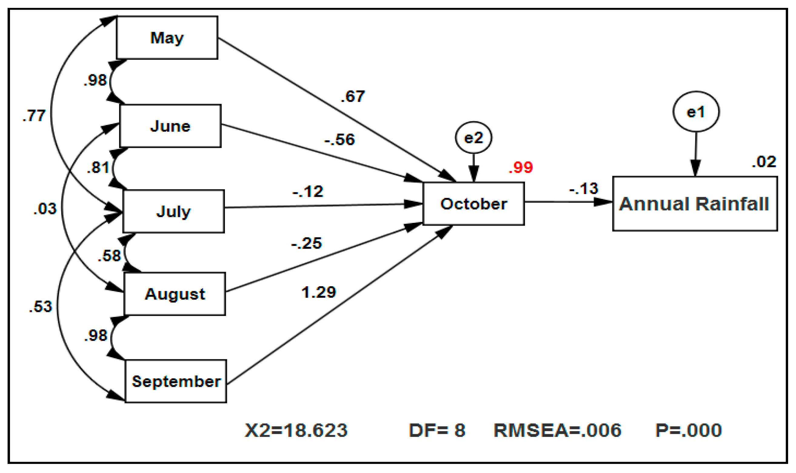
Figure 17.
The effectiveness between the monthly temperature and annual rainfall (fifth model). Monthly effectiveness investigated on annual rainfall series. The effectiveness model shows that six monthly temperature series (May, June, July, August and September) have an indirect effect on annual rainfall. October temperature has a direct effect (negative effect) on annual rainfall ( = 0.99 or 99%, red data).
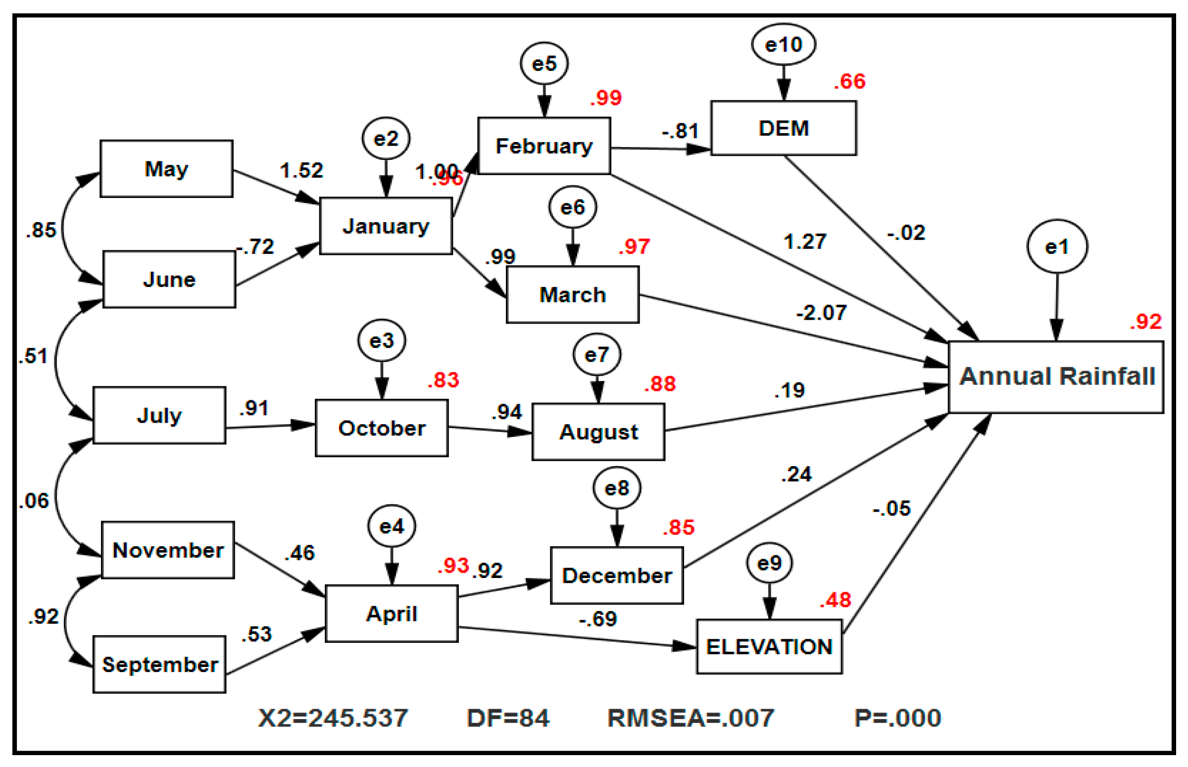
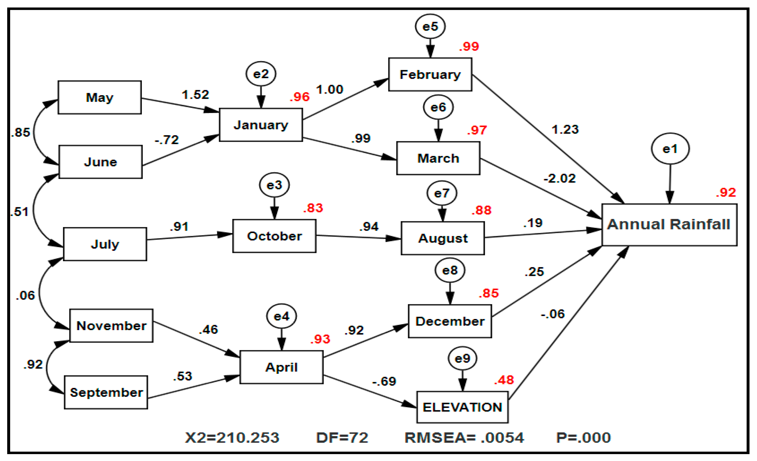
Figure 18.
The effectiveness of the temperatures and elevation on annual rainfall (sixth model). Monthly effectiveness investigated on annual rainfall series. The effectiveness model shows that eight monthly temperature series (January, April, May, June, July, September, October and November) have indirect effects on annual rainfall. February, March, August, December temperatures and elevation have direct effects (negative and positive effects) on annual rainfall (0.48 < R2 < 0.99, red data).
Figure 19.
The effectiveness of the temperatures, elevation, and DEM on annual rainfall (seventh model). Monthly effectiveness investigated on annual rainfall series. The effectiveness model shows that eight monthly temperature series (January, April, May, June, July, September, October and November) have indirect effects on annual rainfall. February, March, August, December temperature series, elevation and DEM have direct effects (negative and positive effects) on annual rainfall (0.48 < R2 < 0.99, red data).
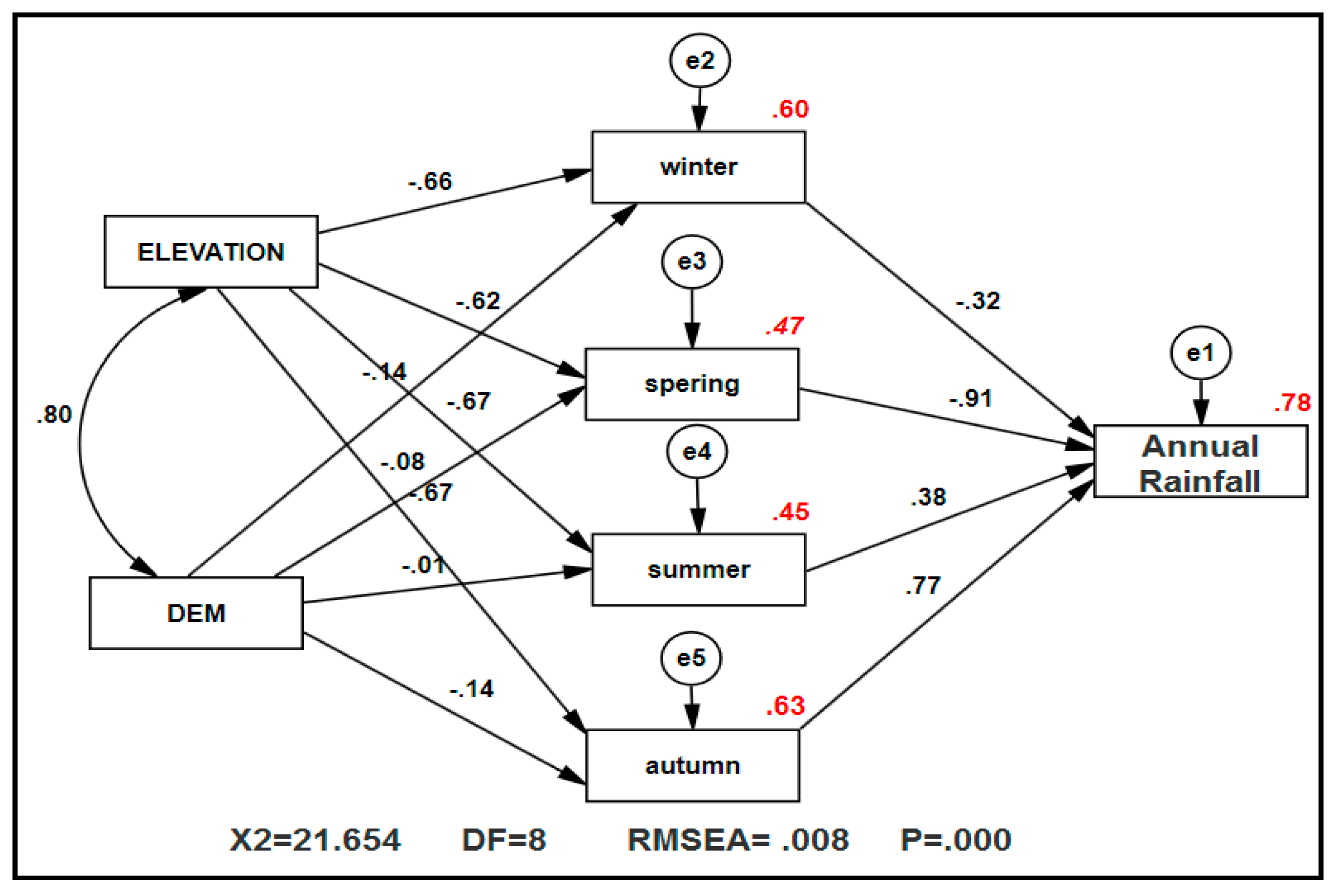
Figure 20.
The effectiveness of the seasonal temperatures, elevation, and DEM on annual rainfall (eighth model). Seasonal effectiveness investigated on annual rainfall series. The effectiveness model shows that seasonal temperature series (winter, spring, summer and autumn) have direct effects on annual rainfall. Elevation and DEM have indirect effects (negative and positive effects) on annual rainfall (0.45 < R2 < 0.60, red data).
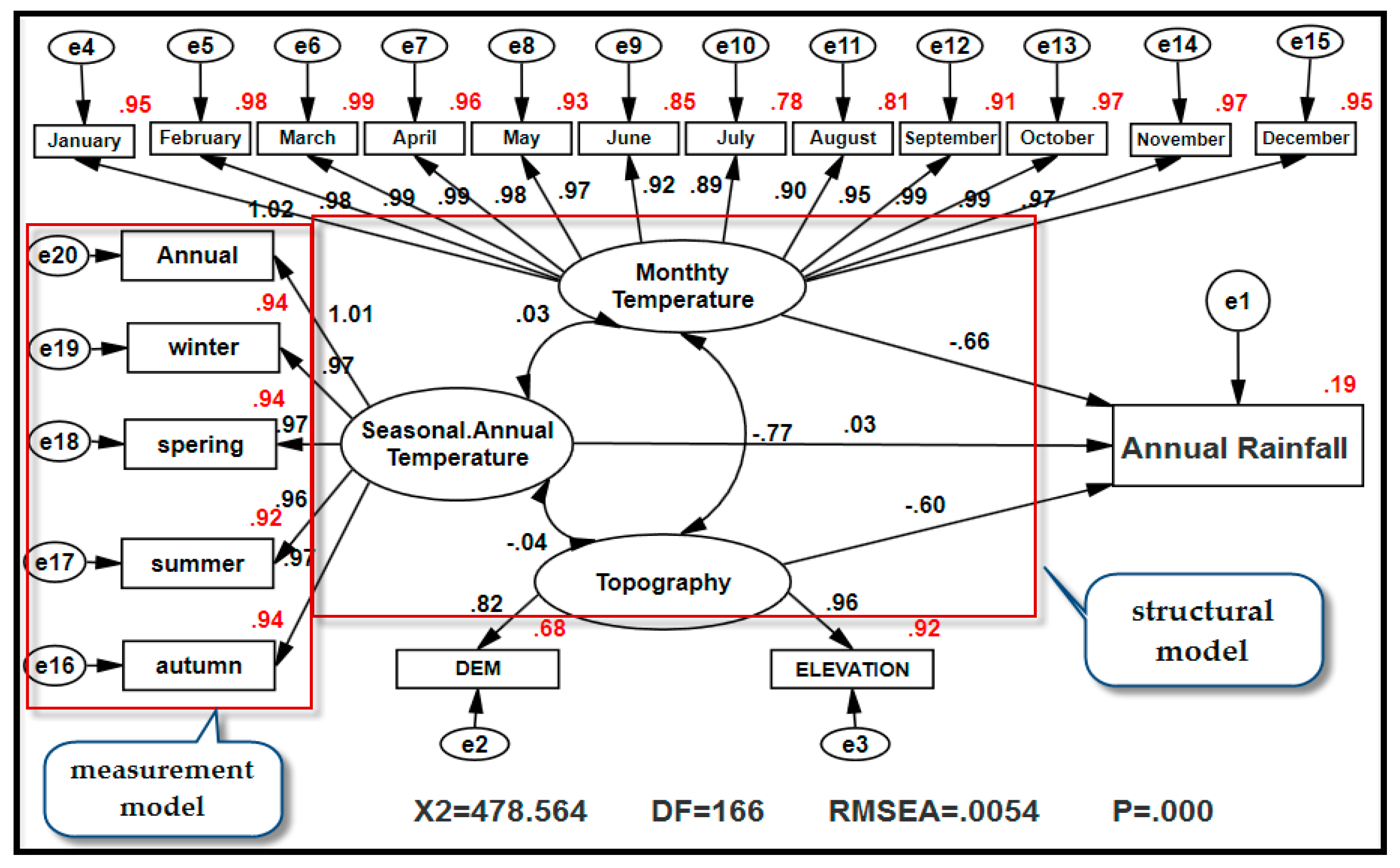
Figure 21.
The effectiveness of the temperatures, elevation, and DEM on annual rainfall (final model). Measurement and structural models analyzed on annual rainfall series. The effectiveness and causality model shows that latent variables or factors (monthly temperature series, seasonal and annual temperature series and topography) have direct (negative effects) and indirect effects (negative and positive effects) on annual rainfall (0.68 < R2 < 0.99, or 68%–99%, red data).
Figure 22.
Forecasting of rainfall by using linear multi-regression.
Figure 22.
Forecasting of rainfall by using linear multi-regression.
Figure 23.
Forecasting of rainfall by using linear multi-regression.
Figure 23.
Forecasting of rainfall by using linear multi-regression.
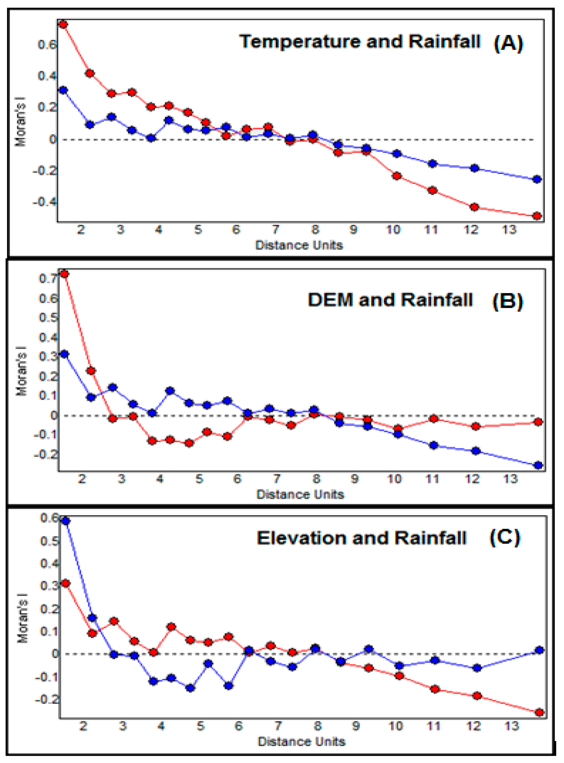
Figure 24.
Illustrates forecasting of the Moran’s I statistics for spatial effectiveness. There is relatively high Moran’s I of 0.25 in the first distance class, indicating that Type Moran’s I errors are biased. More importantly, there is a lack of explanation of richness at those short distances. (A) Temperature and rainfall; (B) DEM and rainfall; (C) Elevation and rainfall.
Figure 25.
Moran’s I statistics of the GWR model.
Figure 25.
Moran’s I statistics of the GWR model.
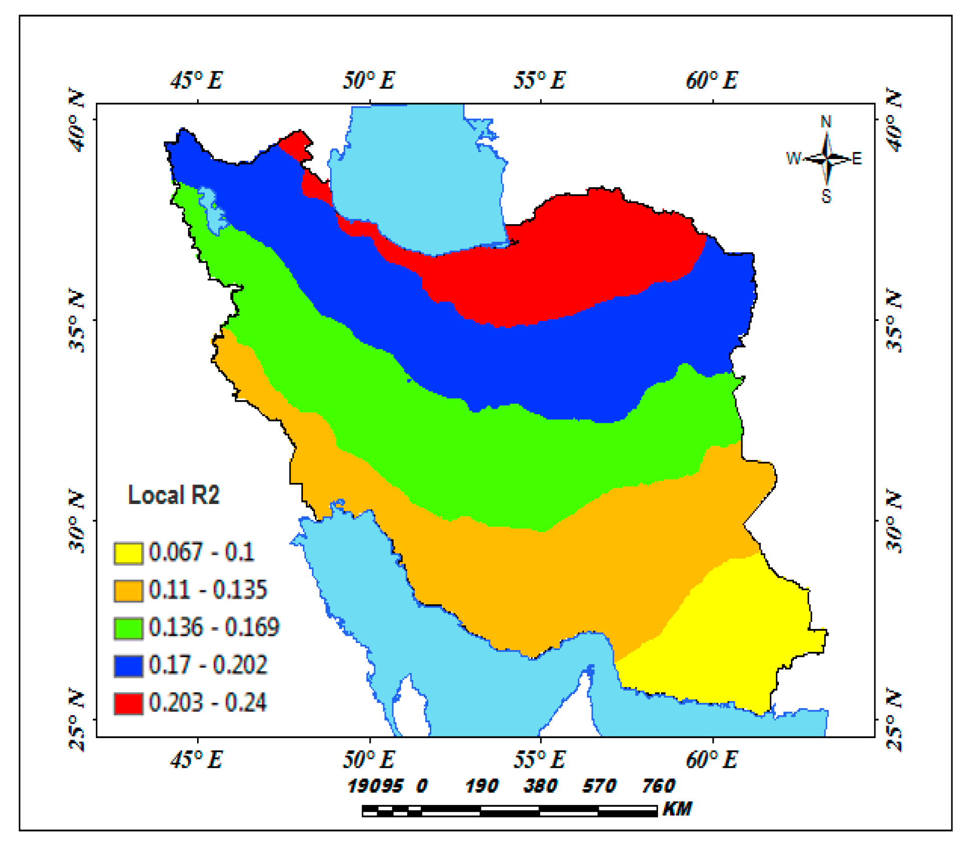
Figure 26.
Local of the GWR model.
Figure 26.
Local of the GWR model.
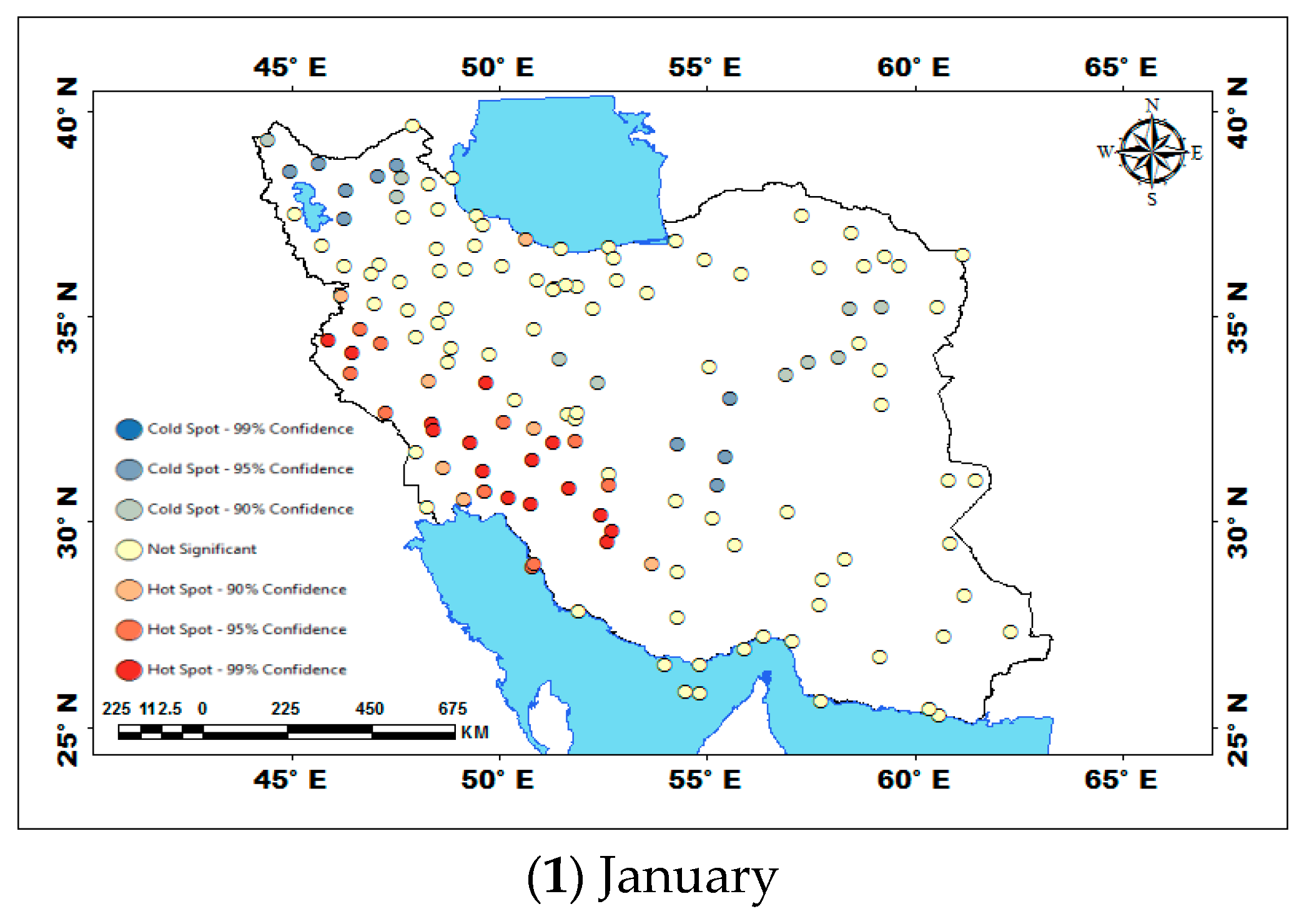
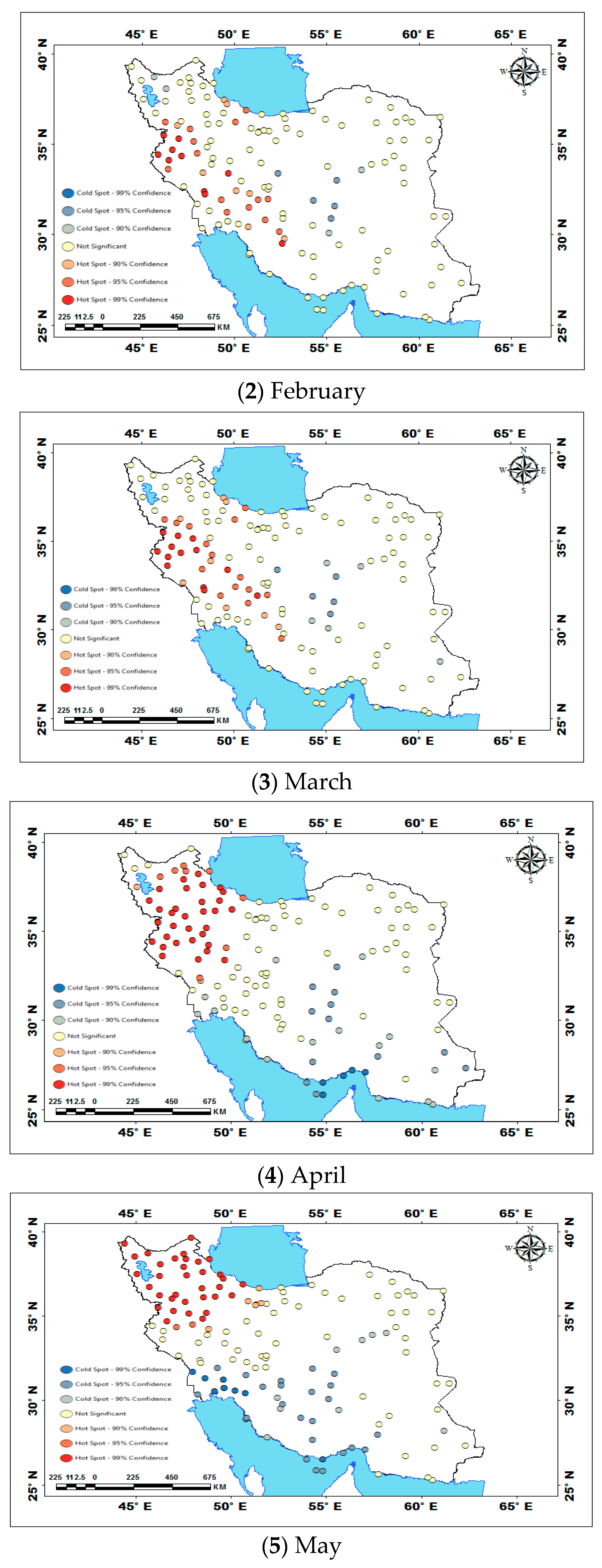
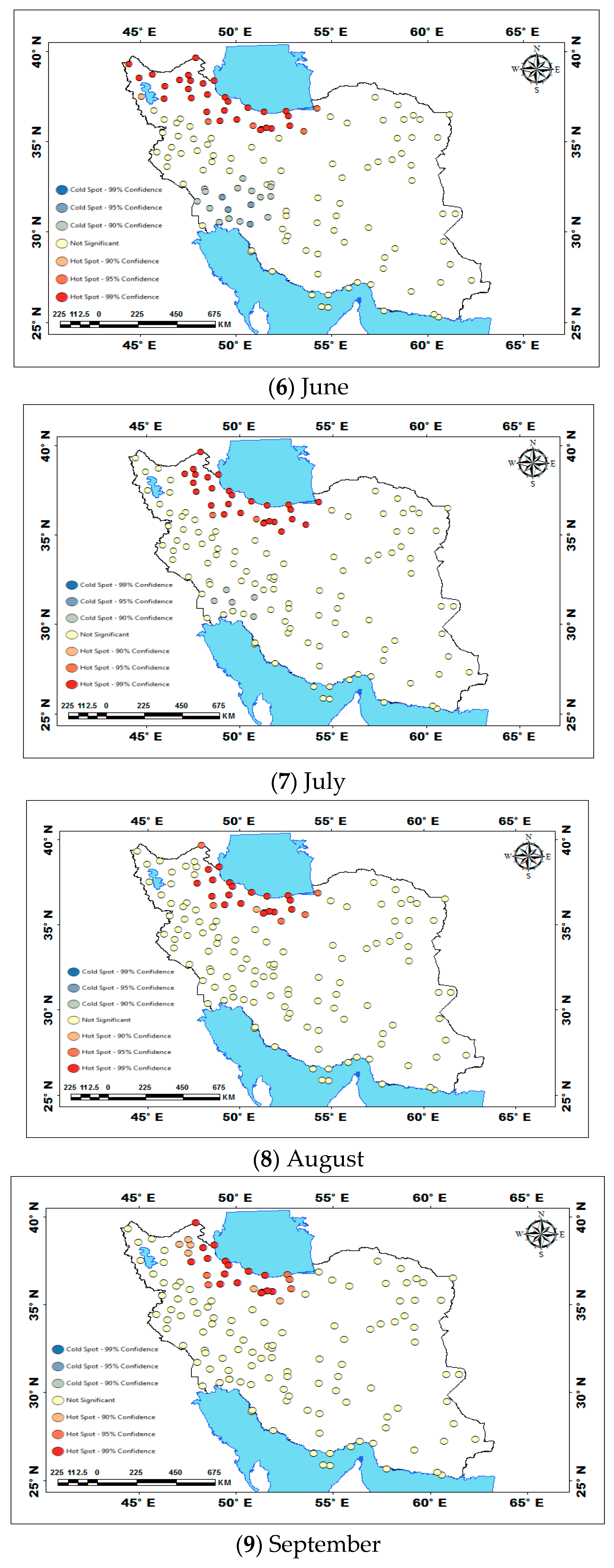
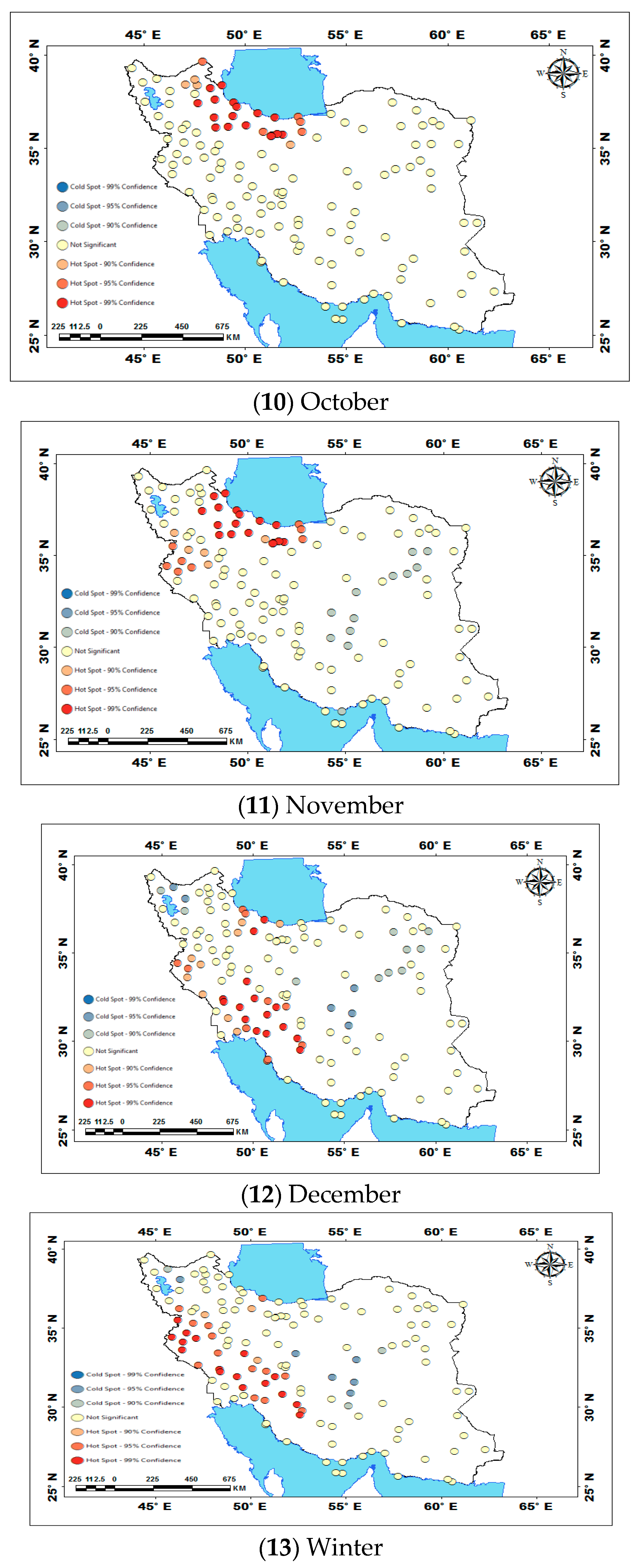
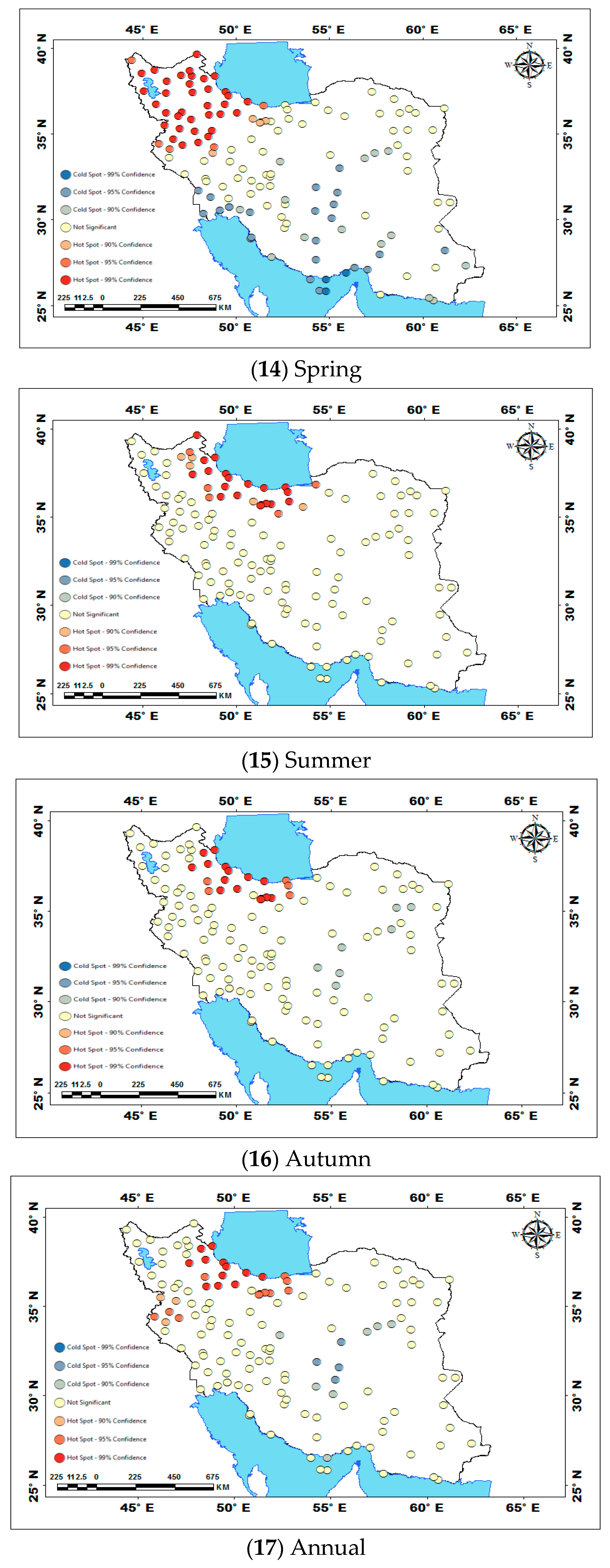
Figure 27.
Gi statistics calculated monthly (1–12), seasonally (13–16) and monthly (17).
Figure 27.
Gi statistics calculated monthly (1–12), seasonally (13–16) and monthly (17).
Table 1.
Statistical properties of original and estimated series.
Table 1.
Statistical properties of original and estimated series.
| Variables | Mean | Standard Deviation (SD) | Relative Standard Deviation % (RSD) | Minimum | Maximum |
|---|
| Annual temperature | 17.8 | 5.37 | 30.1 | 8.60 | 28.60 |
| Estimated temperature | 17.61 | 4.93 | 27.9 | 8.54 | 27.97 |
| Annual rainfall | 322.8 | 280.2 | 91 | 51.3 | 1830.5 |
| Estimated rainfall | 313 | 218.9 | 69.9 | 0.0 | 1496.2 |
| Elevation | 1053.41 | 697.98 | 62.76 | −23.6 | 6105 |
| Estimated elevation | 1139.44 | 619 | 54.32 | −22.8 | 5595 |
Table 2.
The cross-validation of estimated series.
Table 2.
The cross-validation of estimated series.
| Series | ME | RMSE | ASE | RMSSE |
|---|
| OK | SK | IDW | OK | SK | IDW | OK | SK | IDW | OK | SK | IDW |
|---|
| Annual Temperature | −0.1 | −0.13 | −0.17 | 2.13 | 2.205 | 3.11 | 2.46 | 2.89 | 3.54 | 0.985 | 0.996 | 2.01 |
| Winter temperature | −0.09 | −0.06 | −0.12 | 2.1 | 2.24 | 2.36 | 2.62 | 3.46 | 3.67 | 0.88 | 0.73 | 1.04 |
| Spring temperature | −0.06 | −0.14 | −0.211 | 2.32 | 2.386 | 2.63 | 2.94 | 2.89 | 3.15 | 0.798 | 0.93 | 0.976 |
| Summer temperature | −0.02 | −0.17 | −0.21 | 2.4 | 2.31 | 2.46 | 3.13 | 2.38 | 3.42 | 0.77 | 1.65 | 1.73 |
| Autumn temperature | −0.01 | −0.028 | −0.031 | 2.11 | 2.29 | 3.11 | 2.77 | 3.66 | 3.86 | 0.78 | 0.66 | 0.96 |
| Elevation | 16.15 | 34.94 | 38.34 | 375.25 | 379.36 | 385.6 | 194.46 | 494.5 | 499.54 | 0.902 | 0.93 | 1.32 |
| Annual Rainfall | −2.97 | −9.8 | −11.4 | 170.67 | 197.46 | 203.3 | 241.38 | 192.86 | 253.1 | 0.813 | 0.84 | 0.97 |
Table 3.
The significant correlation coefficient.
Table 3.
The significant correlation coefficient.
| Temperature Variable | Estimate or (Regression Weights) | Standard Error (S.E.) | Citical Ratio (C.R.) | P |
|---|
| January | 33.569 | 3.617 | 9.282 | *** |
| February | 18.400 | 1.776 | 10.360 | *** |
| March | 1.000 | 3.024 | 9.248 | *** |
| April | 15.467 | 1.491 | 10.376 | *** |
| May | 27.967 | 3.024 | 9.248 | *** |
| June | −538.782 | 119.484 | −4.509 | *** |
| July | 20.416 | 2.207 | 9.249 | *** |
| August | 843.016 | 121.951 | 6.913 | *** |
| September | 890.964 | 134.886 | 6.605 | *** |
| October | 7.076 | 0.593 | 11.933 | *** |
| November | 1.000 | 1.491 | 10.376 | *** |
| December | 22.709 | 2.431 | 9.343 | *** |
| Elevation | −64,645.096 | 15,338.641 | −4.215 | *** |
Table 4.
The results of the correlation analysis between temperature, elevation and rainfall.
Table 4.
The results of the correlation analysis between temperature, elevation and rainfall.
| Period | R Temperature and Rain | R2% | R Temperature and Elevation | R2% | R Elevation and Rain | R2% |
|---|
| Annual | −0.304 | 1.02 | −0.086 | 59.60 | −0.086 | 3.96 |
| Autumn | −0.101 | 3.72 | −0.772 | 55.80 | −0.199 | 0.48 |
| Winter | −0.193 | 63.84 | −0.747 | 43.30 | 0.069 | 7.67 |
| Spring | −0.799 | 4.80 | −0.658 | 41.73 | 0.277 | 9.73 |
| Summer | −0.219 | 0.42 | −0.646 | 61.31 | −0.312 | 0.88 |
| January | 0.065 | 5.06 | −0.783 | 54.91 | −0.094 | 1.08 |
| February | −0.225 | 17.39 | −0.741 | 48.86 | 0.104 | 4.12 |
| March | −0.417 | 57.76 | −0.699 | 46.10 | 0.203 | 16.97 |
| April | −0.760 | 63.84 | −0.679 | 44.49 | 0.412 | 7.24 |
| May | −0.799 | 22.28 | −0.667 | 37.21 | 0.269 | 3.35 |
| June | −0.472 | 14.98 | −0.610 | 33.99 | −0.183 | 5.48 |
| July | −0.387 | 4.45 | −0.583 | 40.96 | −0.234 | 9.92 |
| August | −0.211 | 2.16 | −0.640 | 48.58 | −0.315 | 10.37 |
| September | −0.147 | 2.82 | −0.697 | 56.10 | −0.322 | 7.13 |
| October | −0.168 | 3.13 | −0.749 | 60.37 | −0.267 | 2.19 |
| November | −0.177 | 0.13 | −0.777 | 59.91 | −0.148 | 1.35 |
| December | 0.036 | 1.02 | −0.774 | 59.60 | −0.116 | 3.96 |
Table 5.
The main effects of rainfall values for all stations (Temperature and Elevation).
Table 5.
The main effects of rainfall values for all stations (Temperature and Elevation).
| Variable | Correlation Coefficient | 95.00% Confidence Interval | t | p-Value |
|---|
| Lower Limit | Upper Limit |
|---|
| Temperature Rainfall | −0.304 | −0.447 | −0.145 | 3.743 | 0.000 |
| Elevation Rainfall | −0.086 | −0.248 | 0.081 | 1.012 | 0.313 |
Table 6.
Significant effectiveness of factors on annual rainfall.
Table 6.
Significant effectiveness of factors on annual rainfall.
| Effectiveness of Factors | Estimate | S.E. | C.R. | P |
|---|
| Annual Rainfall | <--- | Monthly_ Temperature | −33.612 | 6.172 | −5.446 | 000 |
| Annual Rainfall | <--- | Seasonal and Annual Temperature | 1.591 | 1.154 | 1.379 | 0.168 |
| Annual Rainfall | <--- | Topography | −0.274 | 0.059 | −4.642 | 000 |
| effectiveness (<---) | | | | |
Table 7.
Goodness-of-fit indexes of effectiveness final model in Iran.
Table 7.
Goodness-of-fit indexes of effectiveness final model in Iran.
| Index | RMR | GFI | AGFI | TLI | IFI | PNFI | PGFI | AIC | CACI |
| Final model | 0.023 | 0.998 | 0.976 | 0.971 | 0.989 | 0.228 | 0.189 | 286.5 | 224.7 |
| Index | NFI | RFI | CFI | PCFI | ECVI | BIC | NCP | FMIN | MECVI |
| Final model | 0.990 | 0.958 | 0.991 | 0.228 | 0.01 | 234.7 | 28.5 | 0.01 | 0.01 |
Table 8.
Results of the OLS model.
Table 8.
Results of the OLS model.
| Results for Rainfall as a Response Variable. Temperature, Elevation and DEM as Predictor Variables |
|---|
| N: 174, R: 0.399, R2: 0.16, R2adj: 0.145, F: 10.759, P: <0.001 |
| Akanke’s Information Criterion (AICc) : 2453.833 |
| Variable | Coefficient | Standard Coefficient | VIF | Standard Error | t | P-Value |
| Constant | 1235.539 | 0 | 0 | 161.709 | 7.64 | <0.001 | * |
| Temperature | −34.802 | −0.579 | 2.273 | 6.377 | −5.457 | <0.001 | * |
| DEM | −0.264 | −0.55 | 6.191 | 0.084 | −3.146 | 0.002 | * |
| Elevation | 0.003 | 0.008 | 4.748 | 0.065 | 0.053 | 0.958 | |
| Condition Number : 5.061 |
| Mean of Correlation Matrix : 0.763 |
| First Eigenvalue divided by m : 0.843 |
| Asterisks indicate significant tests in the series at P < 0.05. |
Table 9.
Results of OLS and GWR models.
Table 9.
Results of OLS and GWR models.
| GWR | GWR | OLS | OLS | p-Value | Significance Level | Result |
|---|
| Bandwidth | 7.875 | Multiple R-Squared | 0.106 | 0.0903 | P < 0.01 | Model is not Fitted |
| Residual Squares | 11,484,879.597 | Joint F-Statistic | 6.7269 | 0.0002 | P < 0.01 | is statistically significant |
| Effective Number | 8.905 | Joint Wald Statistic | 29.121 | 0.000002 | P < 0.01 | is statistically significant |
| Sigma | 263.753 | Koenker (BP) Statistic | 4.093 | 0.251558 | P < 0.01 | The relationship modeled are consistent |
| AICc | 2441.513 | Jarque–Bera Statistic | 940.606 | 0.000000 | P < 0.01 | is statistically significant |
| 0.2453 | AICc | 2464.561 | | P < 0.01 | Model is Fitted |
| Adjusted | 0.2092 | VIF | | Values(>7.5) | | is statistically significant |
| | | t | 0.376 | P < 0.01 | P < 0.01 | is statistically significant |
Table 10.
Moran’s I autocorrelation statistics in Iran.
Table 10.
Moran’s I autocorrelation statistics in Iran.
| Series | Moran’s I | Z-Score | p-Value | Result |
|---|
| January | 0.702 | 7.07 | 0.0000 | clustering of high values |
| February | 0.719 | 7.23 | 0.0000 | clustering of high values |
| March | 0.732 | 7.36 | 0.0000 | clustering of high values |
| April | 0.784 | 7.87 | 0.0000 | clustering of high values |
| May | 0.835 | 8.37 | 0.0000 | clustering of high values |
| June | 0.794 | 7.79 | 0.0000 | clustering of high values |
| July | 0.813 | 8.17 | 0.0000 | clustering of high values |
| August | 0.839 | 8.43 | 0.0000 | clustering of high values |
| September | 0.823 | 8.27 | 0.0000 | clustering of high values |
| October | 0.784 | 7.88 | 0.0000 | clustering of high values |
| November | 0.732 | 7.36 | 0.0000 | clustering of high values |
| December | 0.667 | 6.72 | 0.0000 | clustering of high values |
| Winter | 0.722 | 7.27 | 0.0000 | clustering of high values |
| Spring | 0.811 | 8.13 | 0.0000 | clustering of high values |
| Summer | 0.832 | 8.36 | 0.0000 | clustering of high values |
| Autumn | 0.729 | 7.34 | 0.0000 | clustering of high values |
| Annual | 0.788 | 7.91 | 0.0000 | clustering of high values |


