
Optimizing the Spatial Resolution for Urban CO2 Flux Studies Using the Shannon Entropy

 ,
,
Abstract
:1. Background Introduction
1.1. Urban-Scale FFCO2 Emissions
1.2. Urban Flux Integration
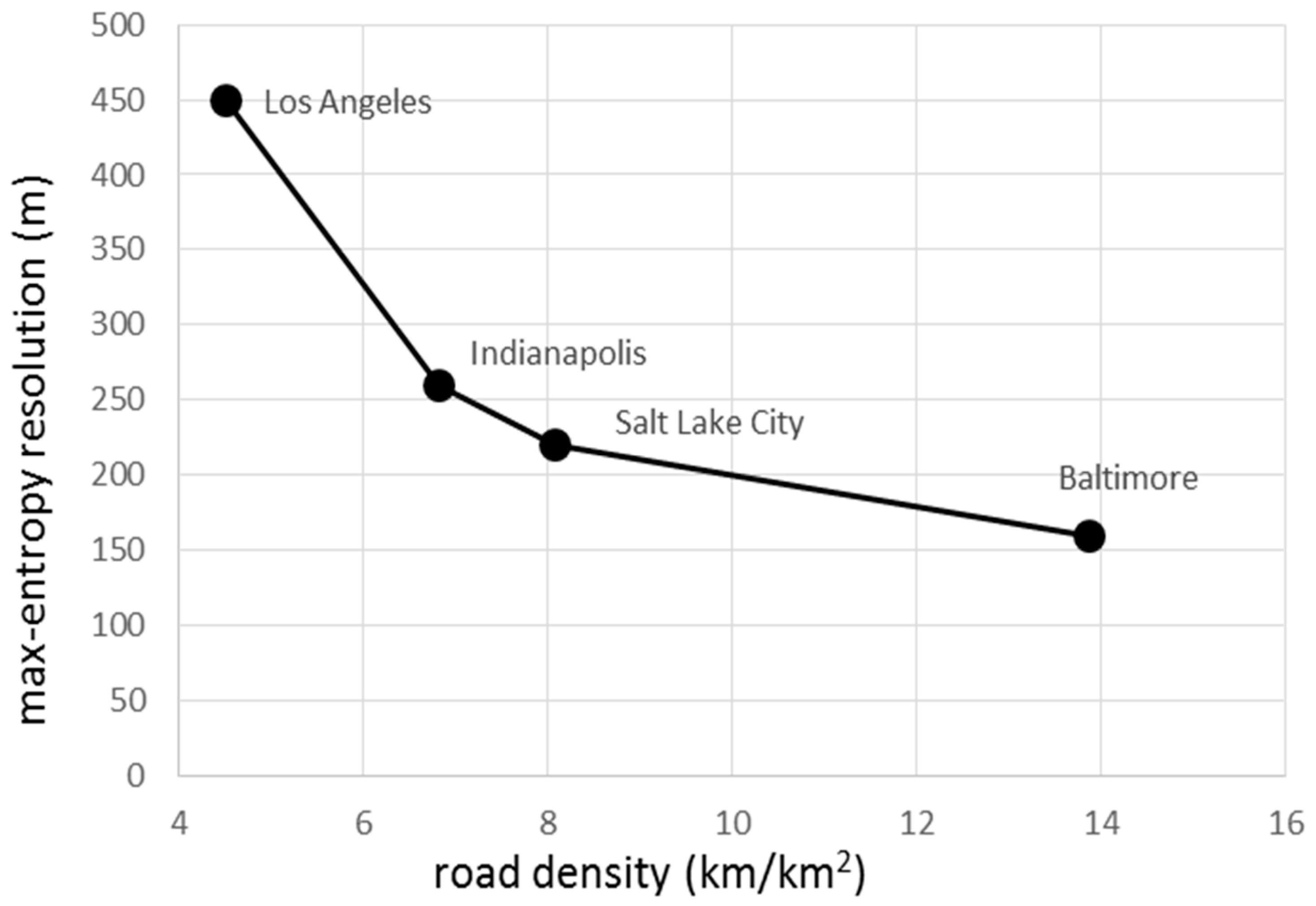
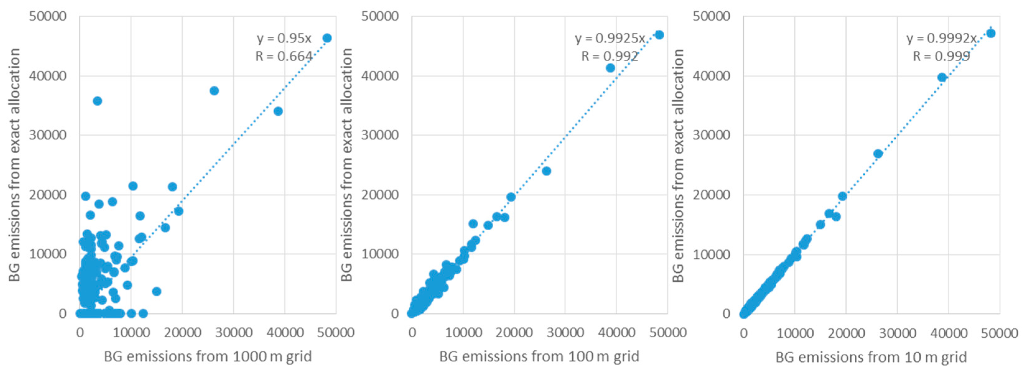
1.3. Grid Scale Optimization
2. Methods
2.1. Application of the Shannon Entropy
2.2. FFCO2 Data
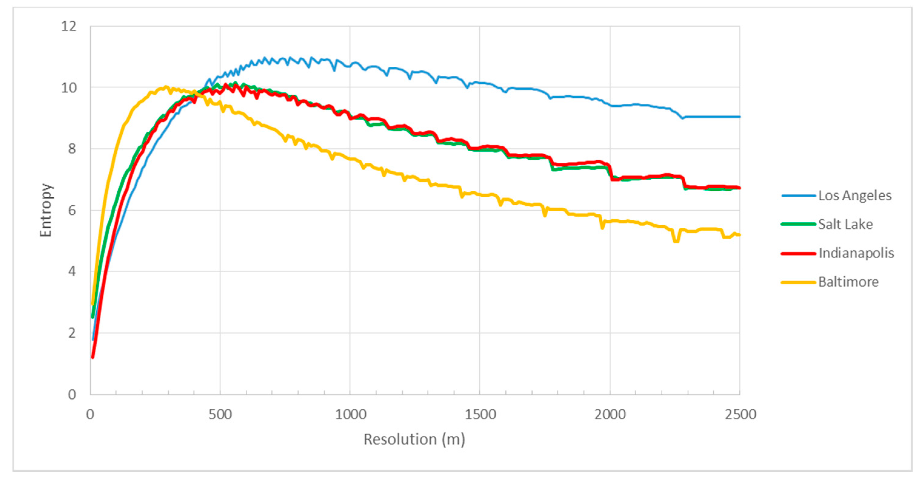
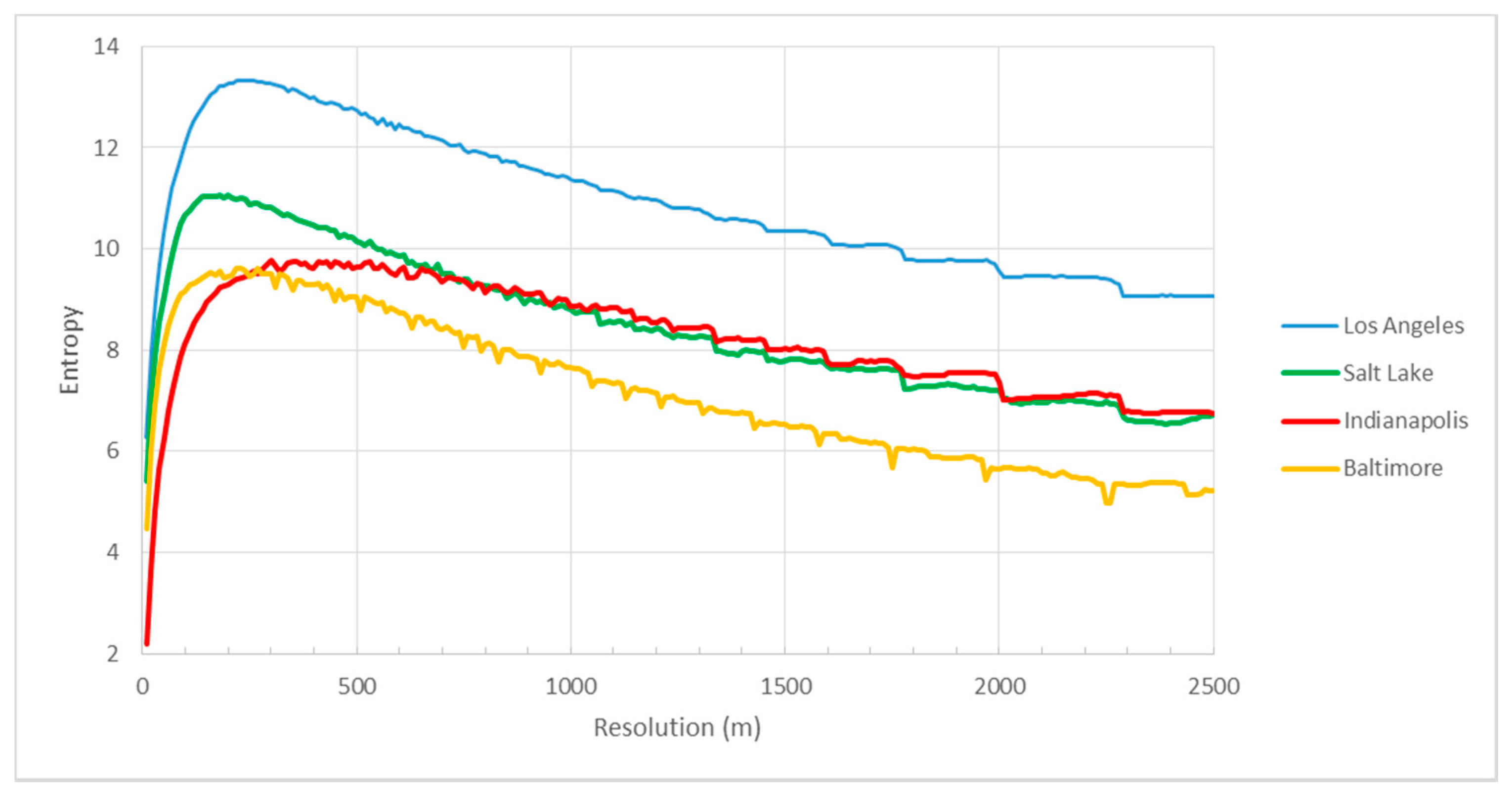
3. Results
4. Analysis and Discussion
5. Conclusions
Acknowledgments
Author Contributions
Conflicts of Interest
References
- Hansen, J.E. Sir John Houghton: Global Warming: The Complete Briefing, 2nd edition. J. Atmos. Chem. 1998, 30, 409–412. [Google Scholar] [CrossRef]
- Gurney, K.R.; Romero-Lankao, P.; Seto, K.C.; Hutyra, L.R.; Duren, R.; Kennedy, C.; Grimm, N.B.; Ehleringer, J.R.; Marcotullio, P.; Hughes, S.; et al. Climate change: Track urban emissions on a human scale. Nature 2015, 525, 179–181. [Google Scholar] [CrossRef] [PubMed]
- Seto, K.C.; Güneralp, B.; Hutyra, L.R. Global forecasts of urban expansion to 2030 and direct impacts on biodiversity and carbon pools. Proc. Natl. Acad. Sci. USA 2012, 109, 16083–16088. [Google Scholar] [CrossRef] [PubMed]
- Romero-Lankao, P.; Gurney, K.R.; Seto, K.C.; Chester, M.; Duren, R.M.; Hughes, S.; Hutyra, L.R.; Marcotullio, P.; Baker, L.; Grimm, N.B.; et al. A critical knowledge pathway to low-carbon, sustainable futures: Integrated understanding of urbanization, urban areas, and carbon. Earth’s Future 2014, 2, 515–532. [Google Scholar] [CrossRef]
- Chester, M.V.; Sperling, J.; Stokes, E.; Allenby, B.; Kockelman, K.; Kennedy, C.; Baker, L.A.; Keirstead, J.; Hendrickson, C.T. Positioning infrastructure and technologies for low-carbon urbanization. Earth’s Future 2014, 2, 533–547. [Google Scholar] [CrossRef]
- Marcotullio, P.J.; Hughes, S.; Sarzynski, A.; Pincetl, S.; Sanchez Peña, L.; Romero-Lankao, P.; Runfola, D.; Seto, K.C. Urbanization and the carbon cycle: Contributions from social science. Earth’s Future 2014, 2, 496–514. [Google Scholar] [CrossRef]
- Hutyra, L.R.; Duren, R.; Gurney, K.R.; Grimm, N.; Kort, E.A.; Larson, E.; Shrestha, G. Urbanization and the carbon cycle: Current capabilities and research outlook from the natural sciences perspective. Earth’s Future 2014, 2, 473–495. [Google Scholar] [CrossRef]
- Bréon, F.M.; Broquet, G.; Puygrenier, V.; Chevallier, F.; Xueref-Remy, I.; Ramonet, M.; Dieudonné, E.; Lopez, M.; Schmidt, M.; Perrussel, O.; et al. An attempt at estimating Paris area CO2 emissions from atmospheric concentration measurements. Atmos. Chem. Phys. 2015, 15, 1707–1724. [Google Scholar] [CrossRef]
- Brioude, J.; Angevine, W.M.; Ahmadov, R.; Kim, S.-W.; Evan, S.; McKeen, S.A.; Hsie, E.-Y.; Frost, G.J.; Neuman, J.A.; Pollack, I.B.; et al. Top-down estimate of surface flux in the Los Angeles Basin using a mesoscale inverse modeling technique: Assessing anthropogenic emissions of CO, NOx and CO2 and their impacts. Atmos. Chem. Phys. 2013, 13, 3661–3677. [Google Scholar] [CrossRef]
- Gurney, K.R.; Razlivanov, I.; Song, Y.; Zhou, Y.; Benes, B.; Abdul-Massih, M. Quantification of fossil fuel CO2 emissions on the building/street scale for a large US city. Environ. Sci. Technol. 2012, 46, 12194–12202. [Google Scholar] [CrossRef] [PubMed]
- Patarasuk, R.; Gurney, K.R.; O’Keeffe, D.; Song, Y.; Huang, J.; Rao, P.; Buchert, M.; Lin, J.C.; Mendoza, D.; Ehleringer, J.R. Urban high-resolution fossil fuel CO2 emissions quantification and exploration of emission drivers for potential policy applications. Urban Ecosyst. 2016, 19, 1013–1039. [Google Scholar] [CrossRef]
- Cambaliza, M.O.L.; Shepson, P.B.; Caulton, D.R.; Stirm, B.; Samarov, D.; Gurney, K.R.; Turnbull, J.; Davis, K.J.; Possolo, A.; Karion, A.; et al. Assessment of uncertainties of an aircraft-based mass balance approach for quantifying urban greenhouse gas emissions. Atmos. Chem. Phys. 2014, 14, 9029–9050. [Google Scholar] [CrossRef]
- Turnbull, J.C.; Keller, E.D.; Baisden, T.; Brailsford, G.; Bromley, T.; Norris, M.; Zondervan, A. Atmospheric measurement of point source fossil CO2 emissions. Atmos. Chem. Phys. 2014, 14, 5001–5014. [Google Scholar] [CrossRef]
- Lauvaux, T.; Miles, N.L.; Deng, A.; Richardson, S.J.; Cambaliza, M.O.; Davis, K.J.; Gaudet, B.; Gurney, K.R.; Huang, J.; O’Keefe, D.; et al. High-resolution atmospheric inversion of urban CO2 emissions during the dormant season of the Indianapolis Flux Experiment (INFLUX). J. Geophys. Res. Atmos. 2016, 121, 5213–5236. [Google Scholar] [CrossRef]
- McKain, K.; Wofsy, S.C.; Nehrkorn, T.; Eluszkiewicz, J.; Ehleringer, J.R.; Stephens, B.B. Assessment of ground-based atmospheric observations for verification of greenhouse gas emissions from an urban region. Proc. Natl. Acad. Sci. USA 2012, 109, 8423–8428. [Google Scholar] [CrossRef] [PubMed]
- Betsill, M.M.; Bulkeley, H. Cities and the multilevel governance of global climate change. Glob. Gov. 2006, 12, 141–159. [Google Scholar]
- Rayner, P.J.; Raupach, M.R.; Paget, M.; Peylin, P.; Koffi, E. A new global gridded data set of CO2 emissions from fossil fuel combustion: Methodology and evaluation. J. Geophys. Res. Atmos. 2010, 115. [Google Scholar] [CrossRef]
- Asefi-Najafabady, S.; Rayner, P.J.; Gurney, K.R.; McRobert, A.; Song, Y.; Coltin, K.; Huang, J.; Elvidge, C.; Baugh, K. A multiyear, global gridded fossil fuel CO2 emission data product: Evaluation and analysis of results. J. Geophys. Res. Atmos. 2014, 119, 10213–10231. [Google Scholar] [CrossRef]
- Gurney, K.R.; Mendoza, D.L.; Zhou, Y.; Fischer, M.L.; Miller, C.C.; Geethakumar, S.; de la Rue du Can, S. High resolution fossil fuel combustion CO2 emission fluxes for the United States. Environ. Sci. Technol. 2009, 43, 5535–5541. [Google Scholar] [CrossRef] [PubMed]
- National Emissions Inventory (NEI). 2011. Available online: https://www.epa.gov/air-emissions-inventories/2011-national-emissions-inventory-nei-data (accessed on 10 February 2017).
- Jones, C.; Kammen, D.M. Spatial distribution of US household carbon footprints reveals suburbanization undermines greenhouse gas benefits of urban population density. Environ. Sci. Technol. 2014, 48, 895–902. [Google Scholar] [CrossRef] [PubMed]
- Jones, C.M.; Kammen, D.M. A Consumption-Based Greenhouse Gas Inventory of San Francisco Bay Area Neighborhoods, Cities and Counties: Prioritizing Climate Action for Different Locations. Bay Area Air Quality Management District. UC Berkeley 2015. Available online: https://escholarship.org/uc/item/2sn7m83z (accessed on 1 January 2017).
- VandeWeghe, J.R.; Kennedy, C.A. A Spatial Analysis of Residential Greenhouse Gas Emissions in the Toronto Census Metropolitan Area. J. Ind. Ecol. 2007, 11, 133–144. [Google Scholar] [CrossRef]
- Zhao, T.; Horner, M.W.; Sulik, J. A geographic approach to sectoral carbon inventory: Examining the balance between consumption-based emissions and land-use carbon sequestration in Florida. Ann. Assoc. Am. Geogr. 2011, 101, 752–763. [Google Scholar] [CrossRef]
- Porse, E.; Derenski, J.; Gustafson, H.; Elizabeth, Z.; Pincetl, S. Structural, geographic, and social factors in urban building energy use: Analysis of aggregated account-level consumption data in a megacity. Energy Policy 2016, 96, 179–192. [Google Scholar] [CrossRef]
- Lauvaux, T.; Pannekoucke, O.; Sarrat, C.; Chevallier, F.; Ciais, P.; Noilhan, J.; Rayner, P.J. Structure of the transport uncertainty in mesoscale inversions of CO2 sources and sinks using ensemble model simulations. Biogeosciences 2009, 6, 1089–1102. [Google Scholar] [CrossRef]
- Thornton, P.E.; Running, S.W.; White, M.A. Generating surfaces of daily meteorological variables over large regions of complex terrain. J. Hydrol. 1997, 190, 204–251. [Google Scholar] [CrossRef]
- Openshaw, S. A geographical solution to scale and aggregation problems in region-building, partitioning and spatial modelling. Trans. Inst. Br. Geogr. 1977, 4, 459–472. [Google Scholar] [CrossRef]
- Openshaw, S.; Rao, L. Algorithms for Reengineering 1991 Census Geography. Environ. Plan. A 1995, 27, 425–446. [Google Scholar] [CrossRef] [PubMed]
- Cockings, S.; Harfoot, A.; Martin, D.; Hornby, D. Maintaining existing zoning systems using automated zone-design techniques: Methods for creating the 2011 Census output geographies for England and Wales. Environ. Plan. A 2011, 43, 2399–2418. [Google Scholar] [CrossRef]
- Batty, M. Spatial entropy. Geogr. Anal. 1974, 6, 1–31. [Google Scholar] [CrossRef]
- Shannon, C.E. A Mathematical Theory of Communication; ACM SIGMOBILE Mobile Computing and Communications Review: New York, NY, USA, 2001; Volume 5, pp. 3–55. [Google Scholar]
- Moeckel, R.; Donnelly, R. Gradual rasterization: Redefining spatial resolution in transport modelling. Environ. Plan. B 2015, 42, 888–903. [Google Scholar] [CrossRef]
- Zhao, J.; Chen, X.; Bao, A.; Zhang, C.; Shi, W. A method for choice of optimum scale on land use monitoring in Tarim River Basin. J. Geogr. Sci. 2009, 19, 340–350. [Google Scholar] [CrossRef]
- Stoy, P.C.; Williams, M.; Spadavecchia, L.; Bell, R.A.; Prieto-Blanco, A.; Evans, J.G.; Van Wijk, M.T. Using information theory to determine optimum pixel size and shape for ecological studies: Aggregating land surface characteristics in Arctic ecosystems. Ecosystems 2009, 12, 574–589. [Google Scholar] [CrossRef]
- Schumann, A.H.; Geyer, J. GIS-based ways for considering spatial heterogeneity of catchment characteristics. Phys. Chem. Earth Part B 2000, 25, 691–694. [Google Scholar] [CrossRef]
- Singh, V.P. Entropy Theory and Its Application in Environmental and Water Engineering; John Wiley & Sons: New York, NY, USA, 2013. [Google Scholar]
- Jost, L. Entropy and diversity. Oikos 2006, 113, 363–375. [Google Scholar] [CrossRef]
- Balzter, H.; Tate, N.J.; Kaduk, J.; Harper, D.; Page, S.; Morrison, R.; Muskulus, M.; Jones, P. Multi-Scale Entropy Analysis as a Method for Time-Series Analysis of Climate Data. Climate 2015, 3, 227–240. [Google Scholar] [CrossRef]
- Schneider, A.; Friedl, M.A.; Potere, D. A new map of global urban extent from MODIS satellite data. Environ. Res. Lett. 2009, 4, 044003. [Google Scholar] [CrossRef]
- Bartholomé, E.; Belward, A.S. GLC2000: A new approach to global land cover mapping from Earth observation data. Int. J. Remote Sens. 2005, 26, 1959–1977. [Google Scholar] [CrossRef]
- Balk, D.L.; Deichmann, U.; Yetman, G.; Pozzi, F.; Hay, S.I.; Nelson, A. Determining global population distribution: Methods, applications and data. Adv. Parasitol. 2006, 62, 119–156. [Google Scholar] [PubMed]
- Zhou, Y.; Smith, S.J.; Elvidge, C.D.; Zhao, K.; Thomson, A.; Imhoff, M. A cluster-based method to map urban area from DMSP/OLS nightlights. Remote Sens. Environ. 2014, 147, 173–185. [Google Scholar] [CrossRef]
- Gately, C.K.; Hutyra, L.R.; Wing, I.S. Cities, traffic, and CO2: A multidecadal assessment of trends, drivers, and scaling relationships. Proc. Natl. Acad. Sci. USA 2015, 112, 4999–5004. [Google Scholar] [CrossRef] [PubMed]
- Oda, T.; Maksyutov, S. A very high-resolution (1 km × 1 km) global fossil fuel CO2 emission inventory derived using a point source database and satellite observations of nighttime lights. Atmos. Chem. Phys. 2011, 11, 543–556. [Google Scholar] [CrossRef]


| City | Total | Residential | Commercial | Onroad |
|---|---|---|---|---|
| Los Angeles | 140 | 240 | 700 | 450 |
| Salt Lake City | 110 | 180 | 540 | 220 |
| Indianapolis | 120 | 300 | 520 | 230 |
| Baltimore | 80 | 220 | 290 | 160 |
© 2017 by the authors. Licensee MDPI, Basel, Switzerland. This article is an open access article distributed under the terms and conditions of the Creative Commons Attribution (CC BY) license (http://creativecommons.org/licenses/by/4.0/).
Share and Cite
Liang, J.; Gurney, K.R.; O’Keeffe, D.; Hutchins, M.; Patarasuk, R.; Huang, J.; Song, Y.; Rao, P. Optimizing the Spatial Resolution for Urban CO2 Flux Studies Using the Shannon Entropy. Atmosphere 2017, 8, 90. https://doi.org/10.3390/atmos8050090
Liang J, Gurney KR, O’Keeffe D, Hutchins M, Patarasuk R, Huang J, Song Y, Rao P. Optimizing the Spatial Resolution for Urban CO2 Flux Studies Using the Shannon Entropy. Atmosphere. 2017; 8(5):90. https://doi.org/10.3390/atmos8050090
Chicago/Turabian StyleLiang, Jianming, Kevin Robert Gurney, Darragh O’Keeffe, Maya Hutchins, Risa Patarasuk, Jianhua Huang, Yang Song, and Preeti Rao. 2017. "Optimizing the Spatial Resolution for Urban CO2 Flux Studies Using the Shannon Entropy" Atmosphere 8, no. 5: 90. https://doi.org/10.3390/atmos8050090