
Improving Residential Wind Environments by Understanding the Relationship between Building Arrangements and Outdoor Regional Ventilation


School of Architecture and Urban Planning, Nanjing University, Nanjing 210093, China
*
Author to whom correspondence should be addressed.
Atmosphere 2017, 8(6), 102; https://doi.org/10.3390/atmos8060102
Submission received: 23 April 2017
/
Revised: 5 June 2017
/
Accepted: 6 June 2017
/
Published: 9 June 2017
(This article belongs to the Special Issue Recent Advances in Urban Ventilation Assessment and Flow Modelling)
Abstract
:This paper explores the method of assessing regional spatial ventilation performance for the design of residential building arrangements at an operational level. Three ventilation efficiency (VE) indices, Net Escape Velocity (NEV), Visitation Frequency (VF) and spatial-mean Velocity Magnitude (VM), are adopted to quantify the influence of design variation on VE within different regional spaces. Computational Fluid Dynamics (CFD) method is applied to calculate VE indices mentioned above. Several residential building arrangement cases are set to discuss the effect of different building length, lateral spacing and layouts on four typical space patterns under wind directions oblique or perpendicular to the main (long) building facade. The simulation results prove that NEV, VF and VM are useful VE indices, which can reflect different features of flow pattern in studied regional domains. Preliminary parametric studies indicate that wind direction might be the most important factor for improving spatial ventilation. When the angle between main building facade and wind direction is more than 30°, ventilation of different exterior spaces could improve evidently. When wind direction is perpendicular to main building façade, decreasing building length can increase NEV of the middle space by 50%, while decreasing lateral spacing would decrease NEV of the intersection space by 35%.
1. Introduction
Exterior wind conditions are important in urban residential areas. Wind flow around buildings can dilute pollutants and remove excess heat, both of which are closely related to people’s health and quality of life. Figure 1 shows examples of typical residential building arrangements in China. These patterns of building arrangements all reflect the considerations of architects regarding block shape, land use, design regulations, aesthetics and even solar access during the design process. Although many studies have revealed that wind environments of exterior spaces strongly depend on the arrangements of the buildings around them, and some studies have established the powerful influence of design variation on the wind environments of exterior spaces [1,2], during the designing process, designers generally adopt the trial-and-error method [3], since the co-relationship between the geometric exterior space and the wind conditions is still unclear. Thus, for the designing purpose, more studies are needed of the relationship between building arrangements and outdoor wind conditions at the micro-scale.
Based on measurements (field and wind tunnel tests) and/or numerical simulations, numerous studies have discussed the influence of building arrangements on exterior wind conditions. In Section 2 of this paper, a literature review reveals that most studies perform their analysis using generic urban geometries, such as aligned and/or staggered arrays of cubes (urban-like building groups) [4,5] or two-row or multi-row long strips (street canyons) [6,7,8]. By varying the distances between buildings, as well as building heights and wind directions, the influence of design changes under different wind directions can be assessed. These Computational Fluid Dynamics (CFD) simulation results have provided a large amount of valuable information. However, it should be noted that most of these studies, such as discussions of building packing densities and frontal area densities, focus on the characteristics of the whole city. These studies might provide overall guidance about urban planning, but, in further design process, more studies are needed to analyze the effects of specific design changes (building length, distance and layouts) on ventilation in different local spaces. It is very important for architects to design building arrangements for different living units. In addition to ventilation studies of urban-like building groups, several recent studies have also discussed the influence of building arrangements on exterior wind environments. These studies have examined building sizes and distances [9], layouts [10,11] and canyon configurations [12]. However, the geometrical models used in these studies simply combine several individual buildings and ignored the effects of surrounding buildings.
Some studies applied the concept of indoor ventilation into urban environments and assessed the ventilation efficiency (VE) of urban areas [13,14,15,16,17]. These studies provided a new perspective from which to assess and improve wind environments of exterior spaces. Our previous study had investigated influence of varying lateral spacing and lengths in residential buildings on VE in various typical outdoor spaces [18]. In that study, three VE indices—purging flow rate (PFR: the effective airflow rate required to purge pollutants from the domain), visitation frequency (VF: the number of times a pollutant enters the domain and passes through it) and air residence time (TP: the time elapsed between when a pollutant enters or is generated in the domain until it exits)—introduced by Bady et al. were adopted by performing calculations using the CFD method. However, the results showed that PFR and TP depend greatly on space volume, as Bady et al. noted [13]. These indices were limited to analyzing the effect of design variations on regional spatial ventilation.
This paper further explores the method of assessing regional spatial ventilation performance using net escape velocity (NEV) as an index for the design of residential building arrangements at an operational level. Furthermore, to fully discuss spatial ventilation performance, spatial mean velocity magnitude (VM) and visitation frequency (VF) are also employed as indices in this study, as they can reflect the air flow rates and recirculation phenomena of the calculated domains. To calculate these ventilation performance indices, CFD simulation with ANSYS-Fluent 13.0 is adopted. In this paper, the multi-residential building district is selected as an example for use in studying ventilation performance, as these districts account for the largest proportion of districts in China today. Five examples of building arrangements are chosen according to the designs typically found in real residential districts. They represent possible design changes in building length, lateral spacing and layout patterns. In consideration of the effect of surrounding buildings, all cases have similar surrounding conditions. The CFD simulations are performed for two directions, south wind (S) θ = 0° and southeast wind (SE) θ = 30°, which means wind direction are perpendicular and non-perpendicular to the building’s main facade.
2. Literature Review on Urban Wind Flow Prediction for Building Arrangement Design
2.1. Influence of Wind Conditions on Building Arrangements
The effects of design variations on urban ventilation have been discussed by many studies in the field of urban forms and street canyons. Among studies of urban form, for example, Mfula et al. [4], using wind tunnel tests, discussed effect of building spacing and density changing on pollutant dispersion. Buccolieri et al. [15] also studied the effect of spacing changes on air exchange rates using numerical modeling. These studies mostly focus on the influence of building density on overall urban wind flows. Therefore, arrays of square buildings are chosen as objects of CFD simulation, with equal longitudinal and lateral spacing used to investigate the influence of spacing variations on pollutant concentration distribution. Buccolieri et al. [19] also chose square arrays when investigating influence of longitudinal and lateral spacing; they showed that variations in spacing perpendicular to wind direction had a more noticeable influence on vertical exchanges of air flow. Similar studies have been performed by Di Sabatino et al. [20], Hang et al. [21,22,23], Ramponi et al. [24], Razak et al. [25] and Lee et al. [26] on building heights, layouts and street widths. In the field of street canyons, as early as 1988, Oke et al. [27] identified three types of characteristic flow based on the width/length (w/h) ratio of street sections. Then, Sini et al. [28], using numerical modeling, discussed different characteristics of wind fields with and without the heating of walls in street canyons of infinite length. They varied w/h ratios of street sections from 0.3 to about 10. CFD simulation results proved the conclusion of Oke et al. [27] and found that wind flow pattern changed radically when windward facade walls are heated. Similar studies were also carried out by Simoëns and Wallace on pollutant dispersion [6,7]. In addition to the w/h ratios of street sections, Chan et al. [29,30] also studied effects of different length/height (l/h) ratio of building facades and building height changes on dispersion of pollutants at different locations. The results showed that non-uniform building heights are beneficial to urban ventilation and that the maximum l/h ratio of building facades should be controlled within the range of 5. Most of these studies have been concerned with proposing a better evaluation method, but their guidance value for design practice is very limited.
In addition, studies related to residential building layouts have been performed in recent years. For example, Hong and Lin [10] compared six layout patterns of multilayer residential buildings under the same density and coverage, and the results showed that layout and orientation of buildings have significant effects on the outdoor wind environment at the pedestrian level. Yang et al. [11] analyzed effect of standard and staggered layouts of roadside multi-floor buildings on the pollutants dispersion. Ying [31] and Iqbal [32] also compared the layout patterns of high-rise residential buildings. However, most of these studies perform CFD simulations by simply combining several individual buildings, without considering the effect of surrounding buildings.
2.2. The CFD Approaches for Urban Wind Flow Modelling
The application of CFD simulation for urban wind flow modelling has developed rapidly in the last 20 years [33]. Compared to wind-tunnel or full-scale testing, CFD simulation method has some important advantages in predicting wind flow around buildings [33,34,35]. In the detailed review of 50 years of computational wind engineering [33], Blocken stated that “They can provide detailed information on the relevant flow variables in the whole calculation domain (‘whole-flow field data’), under well-controlled conditions and without similarity constraints. However, the accuracy and reliability of CFD are of concern and solution verification and validation studies are imperative”.
For wind flow predicting using CFD simulation, Reynolds-Averaged Navier-Stokes (RANS) and Large Eddy Simulation (LES) are two main approaches. RANS approaches include steady RANS and unsteady RANS (URANS). In addition, hybrid RANS/LES approaches also exist, although they are rarely used in urban physics and wind engineering [33]. Studies using these approaches for urban physics have been reviewed by Stathopoulos [34,36], Moonen et al. [37], Blocken et al. [35,38] and Blocken [33,39]. From these reviews, it can be stated URANS are relatively rare adopted in urban flow simulation, as it does not simulate the turbulence, but only its statistics. Moreover, URANS also requires a high-spatial resolution, so it is recommended that LES is directly used to model wind flow. The main limitation of RANS is that it cannot incorporate the transient behavior of separation and recirculation flow of windward edges. LES on the other hand can resolve the large and generally most important turbulent eddies. Thus, it is generally acknowledged that LES can provide more accurate result than steady RANS. However, if the urban wind prediction focused on mean wind speed rather than on an effective wind speed, RANS approach could be sufficient. Thus, Blocken [39] conclude that “It (steady RANS) is by far the most widely used approach in most urban physics focus areas. The reason for this is twofold: (i) the computational expense of LES and (ii) the increased model complexity of LES in combination with the absence of extensive best practice guidelines for LES”.
Some guidelines, such as AIJ (Architectural Institute of Japan) guideline [40] and COSTA (European Cooperation in Science and Technology) action [41], have provided important recommendations of using the CFD technique for appropriate prediction of pedestrian wind environments. In these guidelines, the basic technique demands are provided, including computational domain size, grid and boundary conditions. These demands provide solid bases for our ventilation performance study.
2.3. Assessment of Urban Spatial Ventilation
To assess ventilation of exterior spaces, wind velocity and pollutant concentration are commonly used in previous studies. Ng et al. carry out a series of studies using wind velocity and pollutant concentration as indices to analyze building permeability, frontal area index and air path [42,43,44,45,46]. Some technical guidelines and policies for urban planning in high-density cities are also summarized [47]. Guidelines for residential neighborhoods are also provided by Chan et al. [29,30] and Kubota et al. [48] based on CFD simulation of pollutant concentration and wind velocity.
In addition to the traditional and commonly used indices, in the last ten years, some indoor ventilation indices have been developed to access VE in urban areas. For example, Bady et al. [13] and Kato and Huang [14] introduced some indoor ventilation parameters and developed a series of scales concept for evaluating VE in urban spaces. Through evaluation of several examples, the studies showed that these ventilation indices appear to be a promising tool for urban ventilation study. Hang et al. [16] used some simple idealized city models to explore the effect of urban morphology on the local mean age of the air (the time it takes for urban external “fresh” air to reach a given location). The air exchange efficiency (the frequency, in a certain area, with which air is replaced by outside “fresh” air) in such idealized city models was also studied [22]. Buccolieri et al. [15,19] also proposed a conceptual framework for city breathability. The overall flow rate across boundaries (sides and street top) and the local mean age of air are used to discuss influence of building packing density. Recently, Hang et al. [17] further discussed city breathability in medium-density urban-like geometries using pollutant transport rate and net escape velocity.
3. Residential Building Configurations and Typical Spaces Studied
3.1. Single Residential Building Sizes
At the level of single building (Figure 2a), Liu and Ding classified China’s recently built living units into a number of types and provided the size range for each type [49]. As shown in Figure 2b, in consideration of different family demands, three unit types—two-bedroom (U1), three-bedroom (U2), and four-bedroom (U3) units—are selected in this study. The depth L of living unit equals that of residential building (L = 12 m). Building length W is determined by the combination of the living units, which can be divided into two and multi-unit combination, as shown in Figure 2c. It is also worth noting that, in consideration of economy, living units with larger areas (U3) are generally selected as side units in two-unit and multi-unit groups, which means the minimum W can be set as 30 m. The buildings each have six floors, with a uniform floor height of 2.8 m, for a total height H of 18 m including parapet above and interior-exterior height difference below. The undulation of balconies on southward façade is considered as a uniform single plane to simplify the computation.
3.2. Residential Building Groups
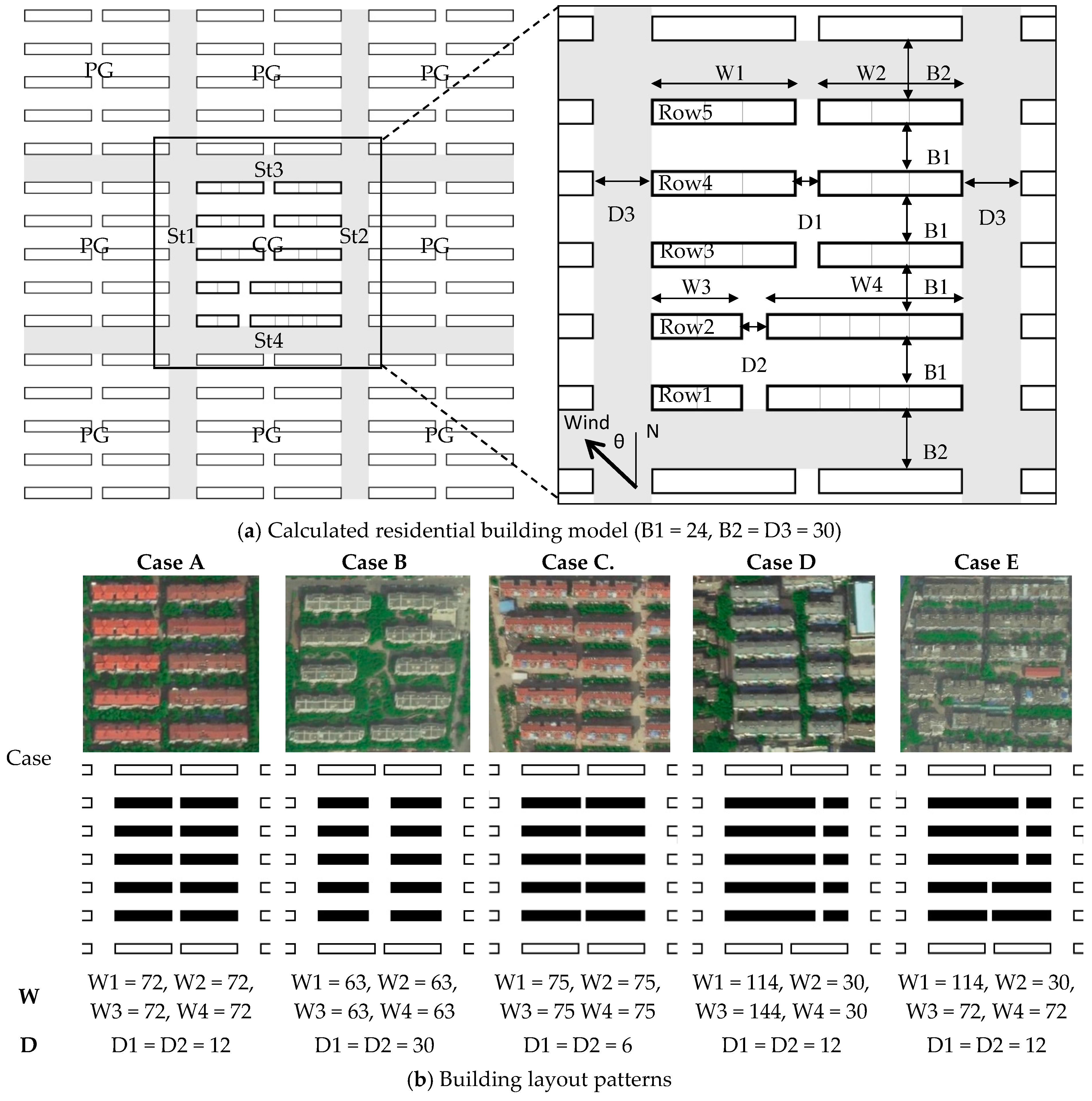
Residential areas in China have common arrangement patterns that are easy to identify and that have resulted from demands for function, sunshine, fire protection and economical use of land resources, as shown in Figure 1. Building groups are uniform strip arrays, such as those in Nanjing City, where up to 65% of residential areas have strip-shaped spacing and slab buildings [50]. Based upon the patterns of existing residential areas, a model of 3 × 3 building groups is set up as the object for CFD simulation, with the central group (CG) providing variation in the configuration analysis and the peripheral groups (PG) setting the environmental conditions, as shown in Figure 3a. The widths (B2 and D3) of the four streets (St1–St4) are determined to be 30 m according to current design code (Figure 3a). For CG, five types are established as study cases for comparison, as shown in Figure 3b, where Case A is set as the initial state and is also chosen as CG building. Building widths in Case A are all determined to be W1 = W2 = 72 m (six units). The longitudinal, namely south–north, spacing B1 is 24 m, which meets the requirement of sunlight spacing, while the east–west spacing is determined as 12 m according to living unit combination and design code. Case B and Case C are both variations developed upon Case A, with consideration of the influences of lateral spacing (D1 and D2) and length variation (W1–W4) on outdoor wind environment. Case D and Case E also follow Case A and discuss the influence of building width and staggering variation on spatial ventilation.
3.3. Ventilation Performance Area and Spatial Patterns
The area selected for data extraction is the space between the third (Row3) and fourth row (Row4) of buildings, as shown in Figure 3a. To compare the effect of variation in design parameters on VE in different areas, some typical domains are selected for comparison, as shown in Figure 4a. These domains could be classified into four spatial patterns, as shown in Figure 4b. RM space stands for the outdoor middle space of the investigated building, and RS space represents the outdoor intersection space; ROD space represents the outdoor outward-side space that adjoins streets St1 and St2; RID space refers to the outdoor inward-side space that adjoins the RS space. The VEs of the four spaces stand for four types of exterior wind environments of dwelling units. The domain volumes of RM (RM1 and RM2), ROD (ROD1 and ROD2) and RID (RID1 and RID2) are invariant, with a uniform size of 12 m wide and 24 m long. The volume of the RS space will vary as the building spacing changes. The domain volume height is from the ground to building height H.
4. Computational Settings of Building Arrangements
4.1. Computational Domain and Boundary Conditions
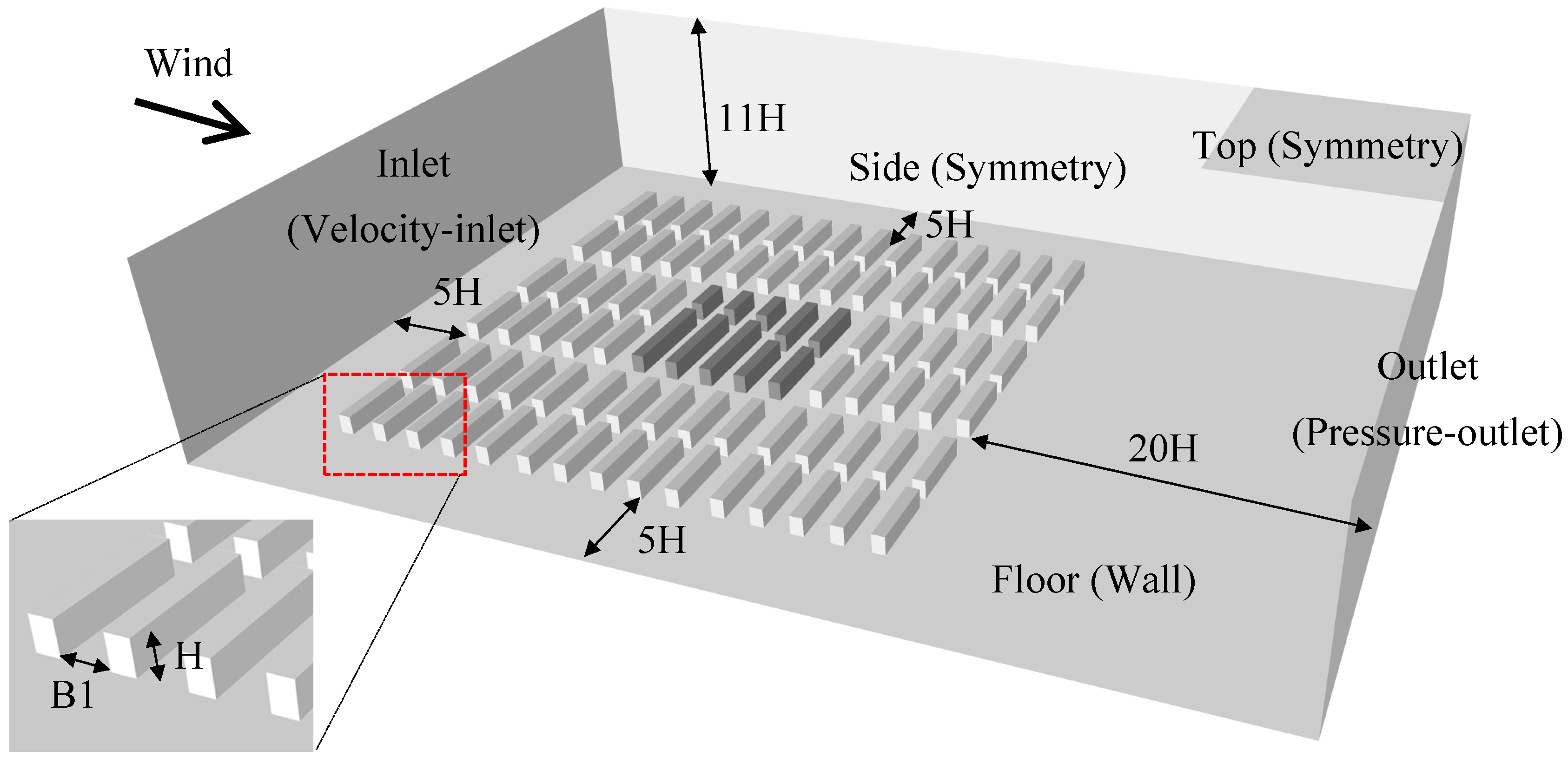
Figure 5 shows the computational domain and boundary conditions in CFD simulation. The domain size refers to AIJ guidelines [40] and some CFD simulation studies of urban ventilation [51,52,53]. The lateral and inflow boundaries are set to 5 H away from the building groups, where H is the uniform building height. The outflow boundary is 20 H away from the building groups and the height of the computational domain is 11 H.
Symmetry boundary conditions, required to enforce a parallel flow, were imposed on the top and lateral sides of the domain. At the outlet boundary of the domain a pressure-outlet condition was used. No-slip wall boundary conditions were used on all solid surfaces. As for the inlet boundary condition, according to AIJ guideline, a power-law velocity profile was applied:
where U(s) is the velocity at reference height, zs, and α is the power-law exponent determined by terrain category. In the development of the AIJ guideline for wind environment prediction, the Working Group carried out some wind tunnel experiments [54]. In these experimental studies, some urban configurations are investigated. The inlet velocity profiles of these studies are adopted in our CFD simulation as they have similar features of urban configuration α = 0.25, and the roughness length z0 is 0.01 m. The thickness of the atmospheric boundary layer is 250 m. The reference wind speed U(s) is 4 m/s at the reference building height zs = H. The turbulent kinetic energy profile (k) and turbulent dissipation rate profile (ε) are calculated as:
where Cμ is a constant (0.09); the friction velocity U* = 0.33 m/s; and κ is the von Karman constant, which is determined to be 0.4.
4.2. Computational Grid and Solver Settings
The computational domain was built using hexahedral elements (about 3.9–4.2 million for different Cases). The grid resolution meets the major computational requirements recommended by Tominaga et al. [40]. As shown in Figure 6, the minimum grid control in direction z is 0.028 H, the minimum grid control in the x and y directions are 0.056 H, and the maximum expansion factor between grids is below 1.25. The grid sensitivity analysis (see Supplementary Material) shows the errors caused by grid resolutions have an unnoticeable effect on the numerical results.
Based on the CFD approaches discussed in previous Section 2.2, the steady RANS approach with standard k-ε turbulence model is adopted in this study. The SIMPLE algorithm is utilized for pressure–velocity coupling. Pressure interpolation is in second order accuracy. For both the convection terms and the viscous terms of the governing equations, second-order discretization schemes are used. Validation study was performed by comparing the CFD simulation results with a wind-tunnel experiment of strip-type building groups (see Supplementary Material). As the experimental building group is different from that used in this study, we built an extra building model, with identical inlet boundary and geometry conditions to those in Zhang et al. [55]. The CFD simulation results, overall, have a good agreement with experimental results.
5. Ventilation Performance of Regional Space
When evaluating the ventilation performance of regional space, PFR and TR are some typical evaluating indices [13,14]. However, the values of these parameters depend greatly on space volume. Unlike indoor space, the boundary of exterior regional space is uncertain, and the determination of space volume is arbitrary. Thus, air flow patterns, i.e., wind velocity and flow recirculation, in the studied domains might be an important aspect of regional spatial ventilation performance. Generally speaking, greater wind velocity and less recirculation could be beneficial for space ventilation. Recently, Lim et al. [56] presented a new concept of the ventilation index, NEV, which is the velocity that corresponds to PFR. Compared to traditional parameters of wind velocity, NEV reflects the effective and net contaminant transport and dilution velocity, which relate not only to the wind speed but also to the flow reversal. Hang et al. [17] further adopted the parameter of net escape velocity to access the influence of city size, building height variations and wind direction for the entire pedestrian volume (throughout the z = 0–2 m volume). By assuming that the pollutant source is generated homogeneously in the studied regional space, the net escape velocity of this space can be calculated using Equation (1) [17]:
where Vol is the studied volume (m3), and <C> is the spatially averaged concentration in the studied volume (kg/m3). Sc is the release rate of uniform pollutants (kg/m3-s). In Hang’s study, Ap is defined as the entire area of boundaries for the entire studied (pedestrian) volume in urban areas. However, using the entire area of boundaries to calculate the NEV could lead to lower NEV values, especially when assessing spaces with large lateral areas, i.e., cross section spaces. From the NEV discussion in Lim et al. [56], we find that it might be more appropriate to define Ap as the normal outflow area of the space’s boundary openings. In this study, we will explore the feasibility of this method to assess the ventilation efficiencies of different spaces.
In addition to NEV, we also employ wind VM and VF as the evaluating parameters to access the air flow pattern in the studied domain. VM and VF can be calculated using Equations (2) and (3) [13,16]:
where Δqp is the inflow flux of pollutants into the domain (kg/s). V is the velocity magnitude. By applying the above concepts, this paper quantifies the effects of design variations for different regional spaces and wind directions on the air flow patterns and the space’s ventilation capacity.
6. Comparison of Ventilation Efficiency in Different Spaces
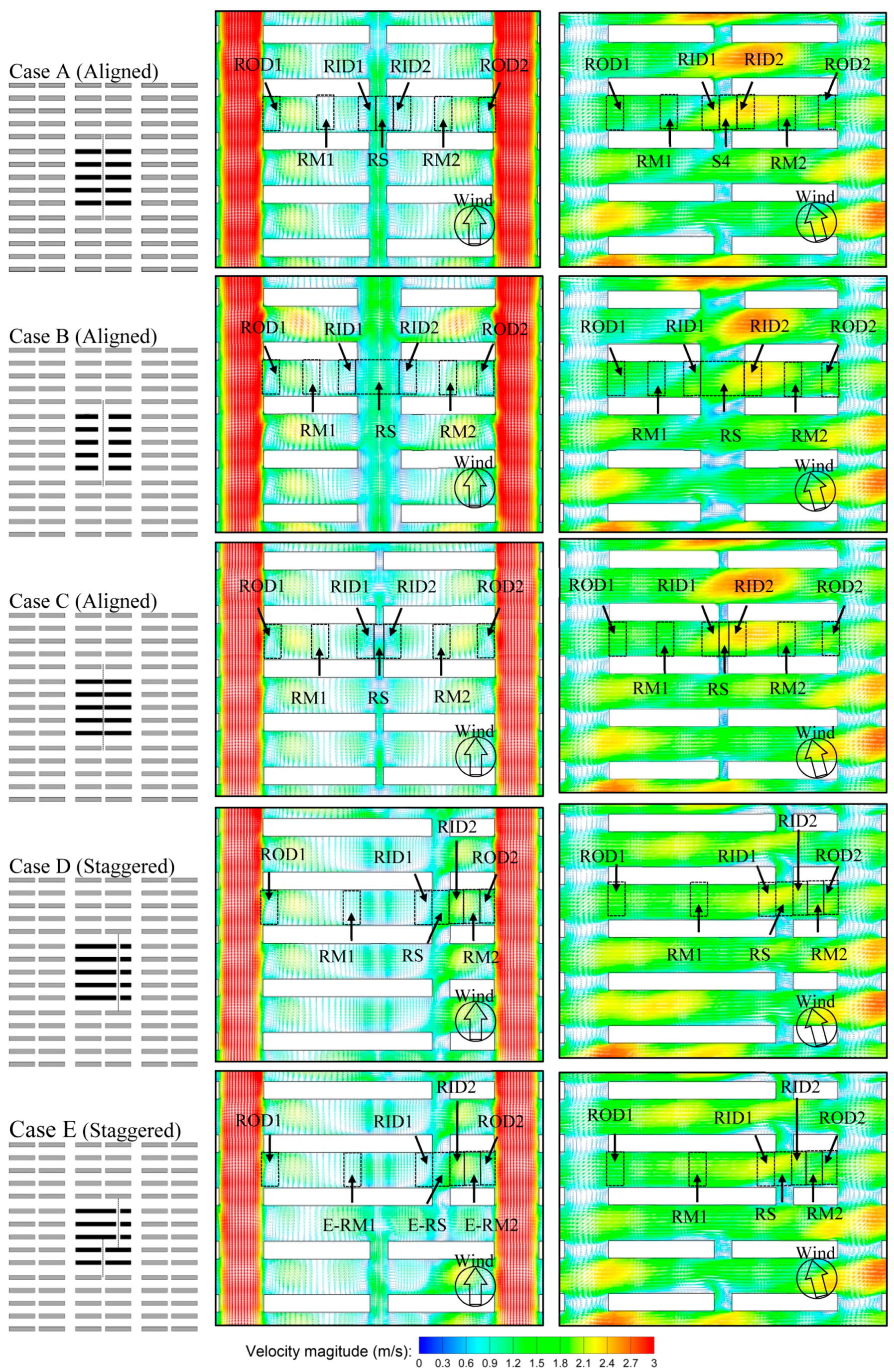
Figure 7 shows the simulation result of wind flow fields for the five cases under two wind directions (θ = S 0° and θ = SE 30°). It reveals that under wind direction θ = S 0°, wind flows pass through the south–north streets and permeate into the spaces between long-strip buildings. The wind flow velocity and recirculation feature of the studied domains varies greatly. Wider streets (St1 and St2) could generally improve the wind velocity of space adjoined to the streets. However, under the wind direction θ = SE 30°, the air flow velocity of different domains improved evidently.
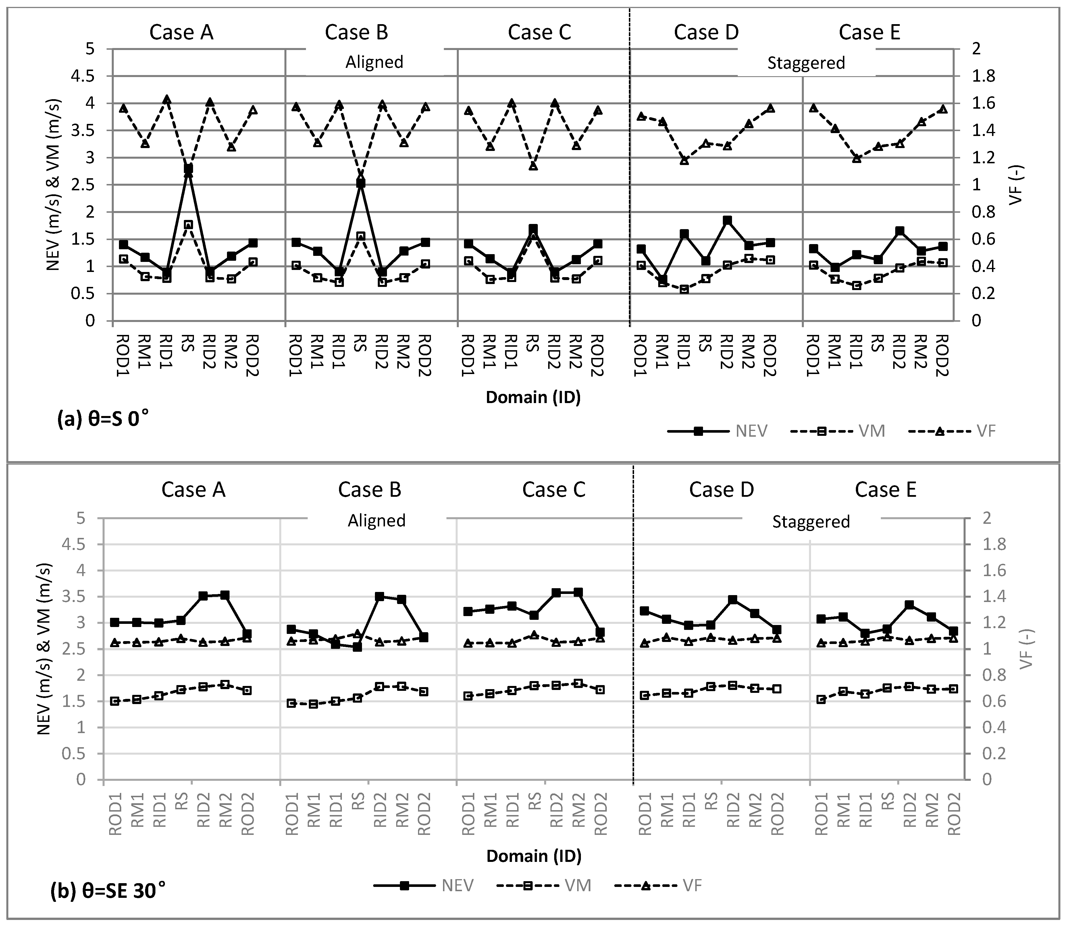
Based on the calculated flow fields, NEV and VF of studied domains are calculated by setting pollutant source generated homogeneously within the study domains (Figure 4). Figure 8 shows the calculated NEV, VF and VM for different domains under wind directions θ = S 0° and θ = SE 30°. From the simulation results, it can be found that wind direction could influence VE of different outdoor spaces greatly. As wind direction θ varies from S 0° to SE 30°, VM of ROD1 and RID1 domains of case A, for example, increased by 33% and 106% respectively. The cause is the strip-shaped outdoor spaces, which forms a ventilation corridor between the southward oriented buildings, allowing increasing airflow into the spaces between, with the wind direction angle changing from perpendicular to parallel to the main building facades. Meanwhile, the VF descends remarkably the other way, especially in spaces near the lateral (ROD1 and ROD2, RID1 and RID2). For example, VF of ROD1 and RID1 domain drops to 1.04 and 1.05, respectively, from 1.57 and 1.63, as wind direction θ varies from S 0° to SE 30°. As a combined effect of the two results above, NEV increases considerably, which shows improvement in ventilation conditions resulting from the wind direction. Therefore, the local prevailing wind direction needs to be included in the design process to maintain a certain angle between the wind and the main building façade for effective improvement of outdoor ventilation.
Under wind condition θ = S 0°, VE indices of different spaces differ noticeably from one another in both values and range. The ventilation efficiency shows a similar variation tendency under the aligned (Case A, Case B, and Case C) and staggered (Case D and Case E) conditions. Under the aligned condition, RS space shows relatively better VE. NEV could reach a more than 20% increase over that of the other three spaces (RM, ROD and RID) (Figure 8a). In these spaces, wind flows pass through the space directly, with relatively high VM and low VF. NEV of the ROD (ROD1 and ROD2) and RID (RID1 and RID2) spaces varies greatly, as shown in Figure 8a. Compared to ROD spaces, RID spaces show the worst VE. VFs of the two spaces are approximately 1.6. However, VM of ROD spaces (ROD1 and ROD2) is much larger than that of RID spaces (RID1 and RID2). This difference is mainly due to the widening of street width (St1 and St2) beside the space. Compared to the ROD and RID spaces, NEV of the RM space (RM1 and RM2) is in the middle, due to the combined effect of lower VF and low mean VM. Under the staggered conditions, NEV of the RID space decreased greatly compared to that under the aligned conditions, mainly due to the effect of staggered buildings, which leads to the great decrease in wind velocity.
Under wind direction θ = SE 30°, NEVs of different spaces do not change very much (Figure 8b). In general, the VE of spaces on the upwind side (RM2, ROD2, and RID2) is better than that of spaces on the downwind side (RM1, ROD1 and RID1). This is mainly because VMs of spaces on the upwind side (RID2–ROD2) are better than that of spaces on the downwind side, and VFs of these spaces do not change very much.
7. Effect of Design Change on Spatial Ventilation Efficiency and Its Related Pollutant Dilution
7.1. Effect of Design Change in Middle Space RM
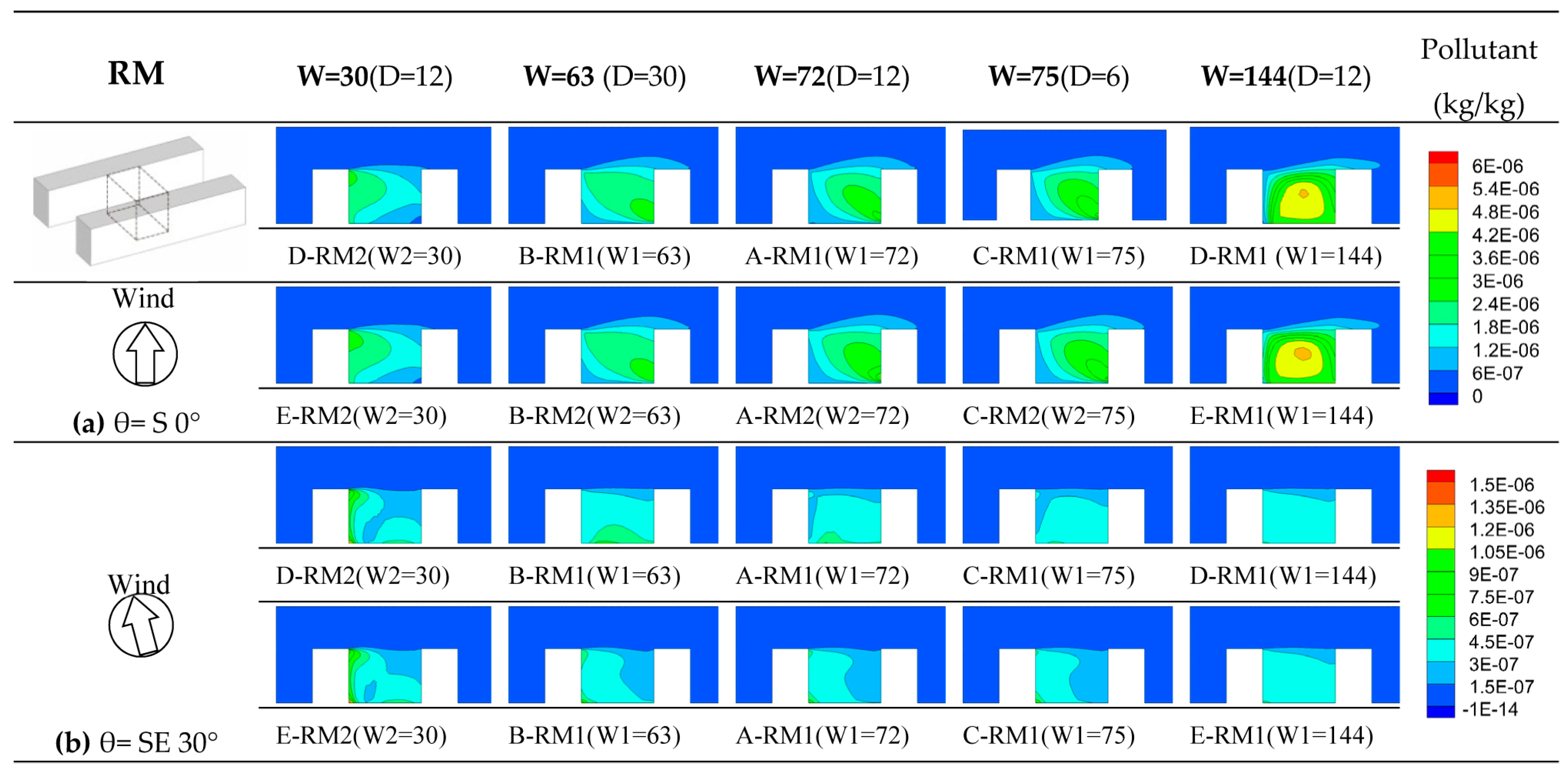
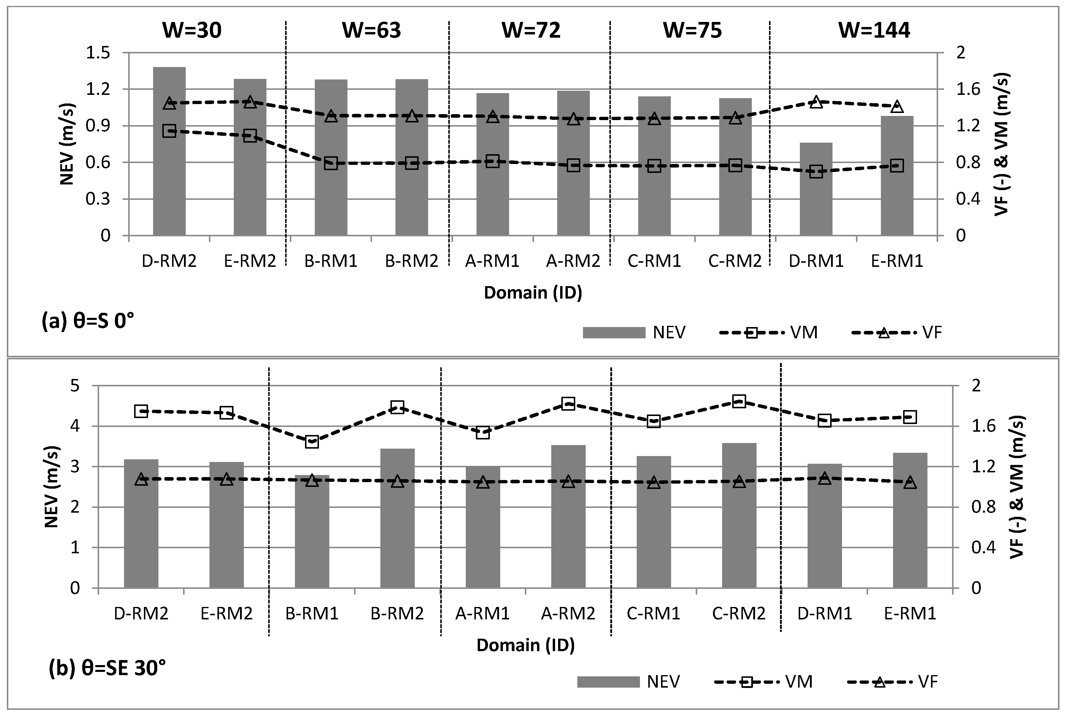
Figure 9 shows the concentration fields within space RM (RM1 and RM2) for different building lengths, spacing distance and staggered conditions under wind directions θ = S 0° and θ = SE 30°. From the simulation results, it can be seen that comparing to building spacing and staggered condition, building lengths might be more relevant to the outdoor ventilation of the RM spaces under wind direction θ = S 0°. In Figure 9a, the pollutant concentrations in the study domains generally increase as building length W increases. As W increases, mean VF of the RM space decreases, and pollutant VFs are around 1.4. These values can be observed in Figure 10a. In this figure, when W = 30 (i.e., in Case D), VM of RM space in case D (D-RM2) increases by approximately 44.5%, 49.1% and 49.5%, respectively, from its values at RM2 in case B, Case A and Case C, where building lengths are 62 m, 73 m and 75 m. When W = 30, VF of space RM in case D (D-RM2) is also larger than that in case B (W = 63), Case A (W = 72) and Case C (W = 75). This reflects the strengthening of wind flow recirculation in these domains as the building length increases. However, when W = 30, VF of the RM space in case D (D-RM2) is also larger than that in Case A, Case B and Case C. This is mainly because building length is 30 m and the RM space (D-RM2) is close to ROD space, where VF is much larger (above 1.4). Under the combined effect, NEV of RM space in Case D (when W = 30) is obviously lower than that in Case A, Case B and Case C. NEV of the RM space in Case E is similar to that in Case D.
Under wind direction θ = SE 30°, the level of pollutant concentration is much lower than that under wind direction θ = S 0°, as shown in Figure 9b. It is mainly due to the improvement of air flow conditions in these studied domains. From Figure 10, it can be seen that when wind direction varies from south 0° to southeast 30°, VM of the RM spaces generally increases from 1 m/s to 1.8 m/s, and VF decreases from 1.4 to 1.04, which shows the great improvement in wind removal efficiency. Under these combined effect, the NEV of RM spaces improves evidently, increasing by about 180%. In addition, the distribution of pollutant concentration in the RM2 space of Case D and Case E is less uniform than that in the RM1 and RM2 spaces of other cases. The cause might be that the wind direction is form southeast, and when building length is 30 m, RM2 space is closely adjacent to the building’s east corner space, at which more recirculation flow occurs.
7.2. Effect of Design Change in Intersection Space RS
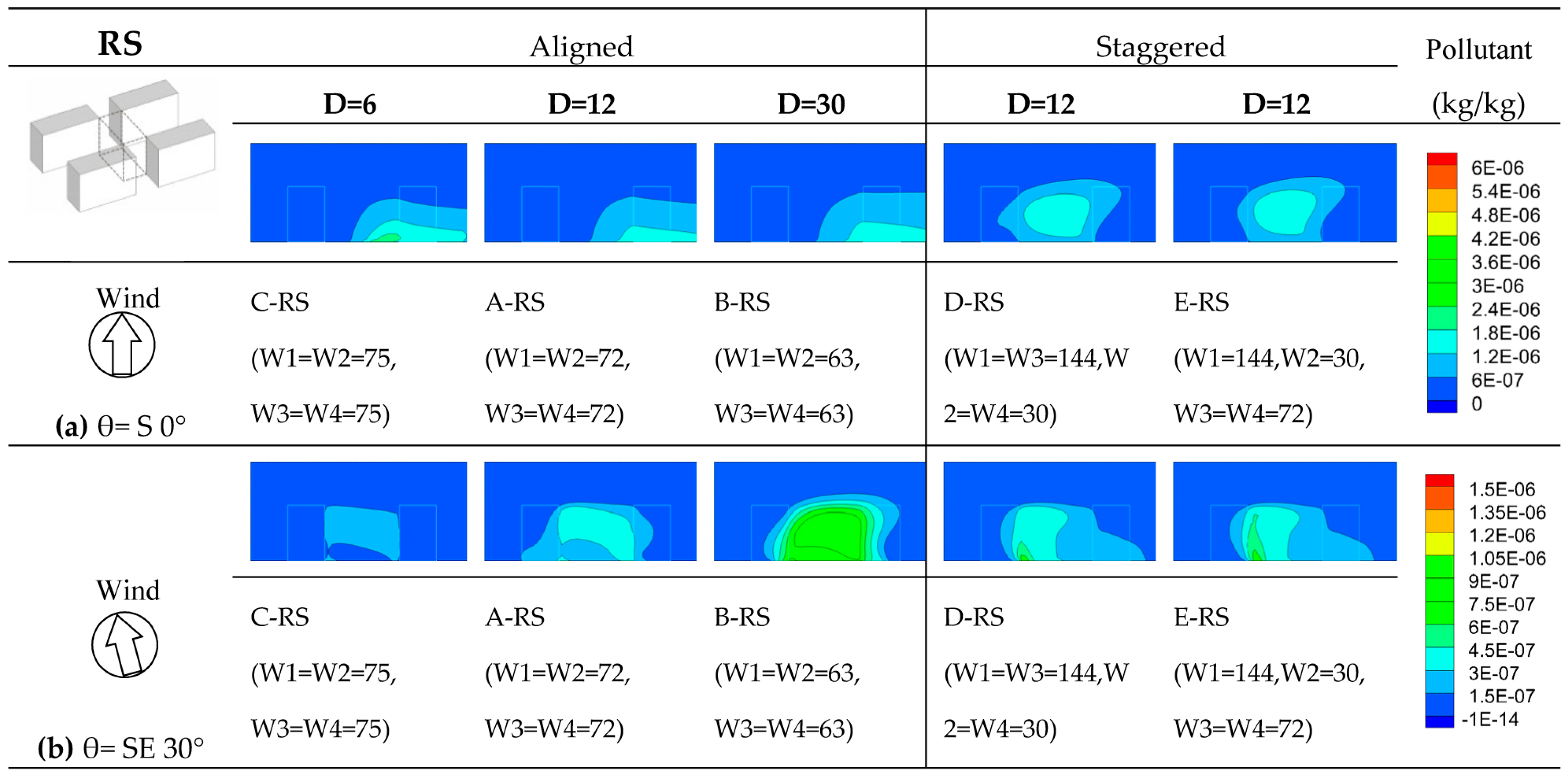
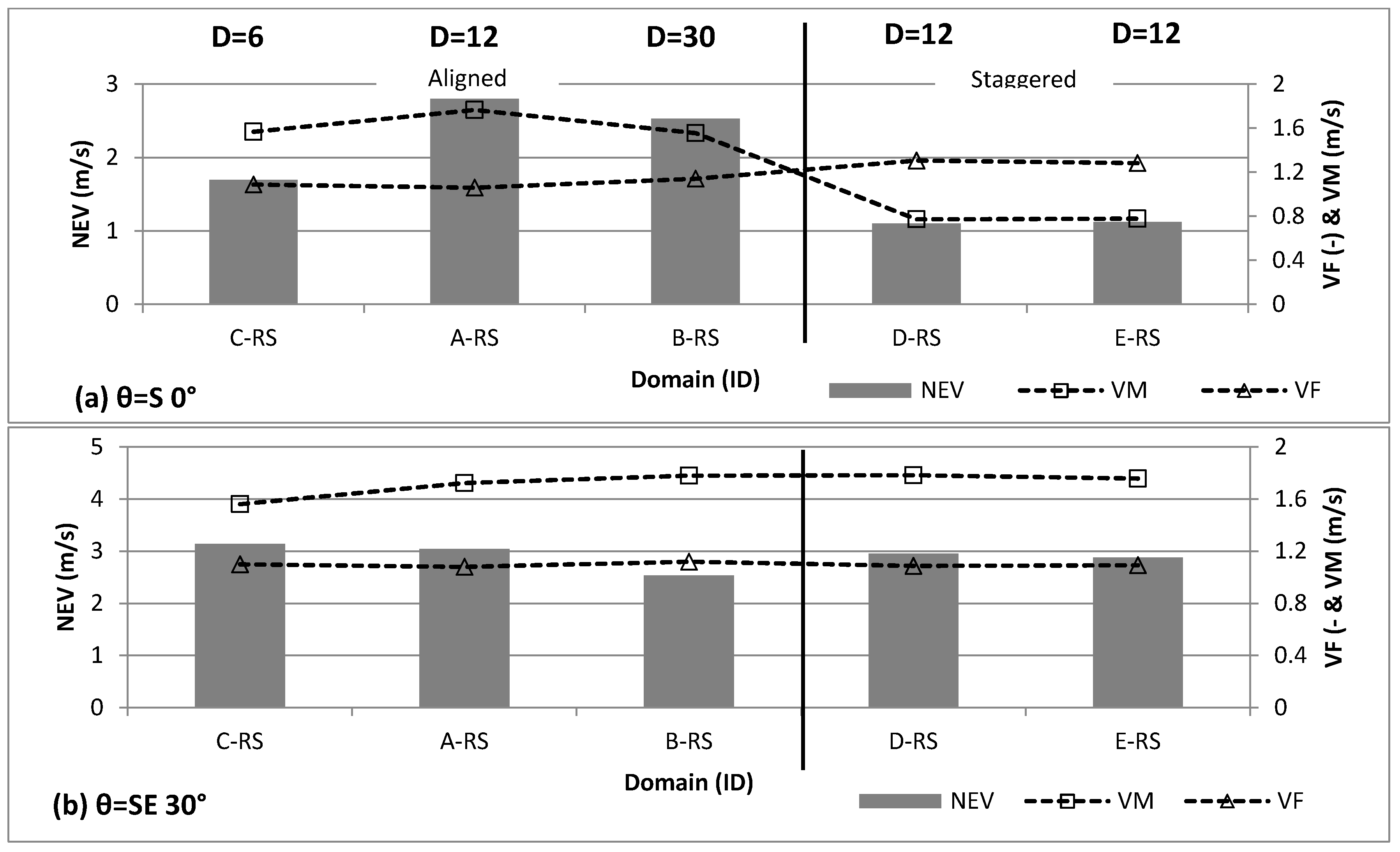
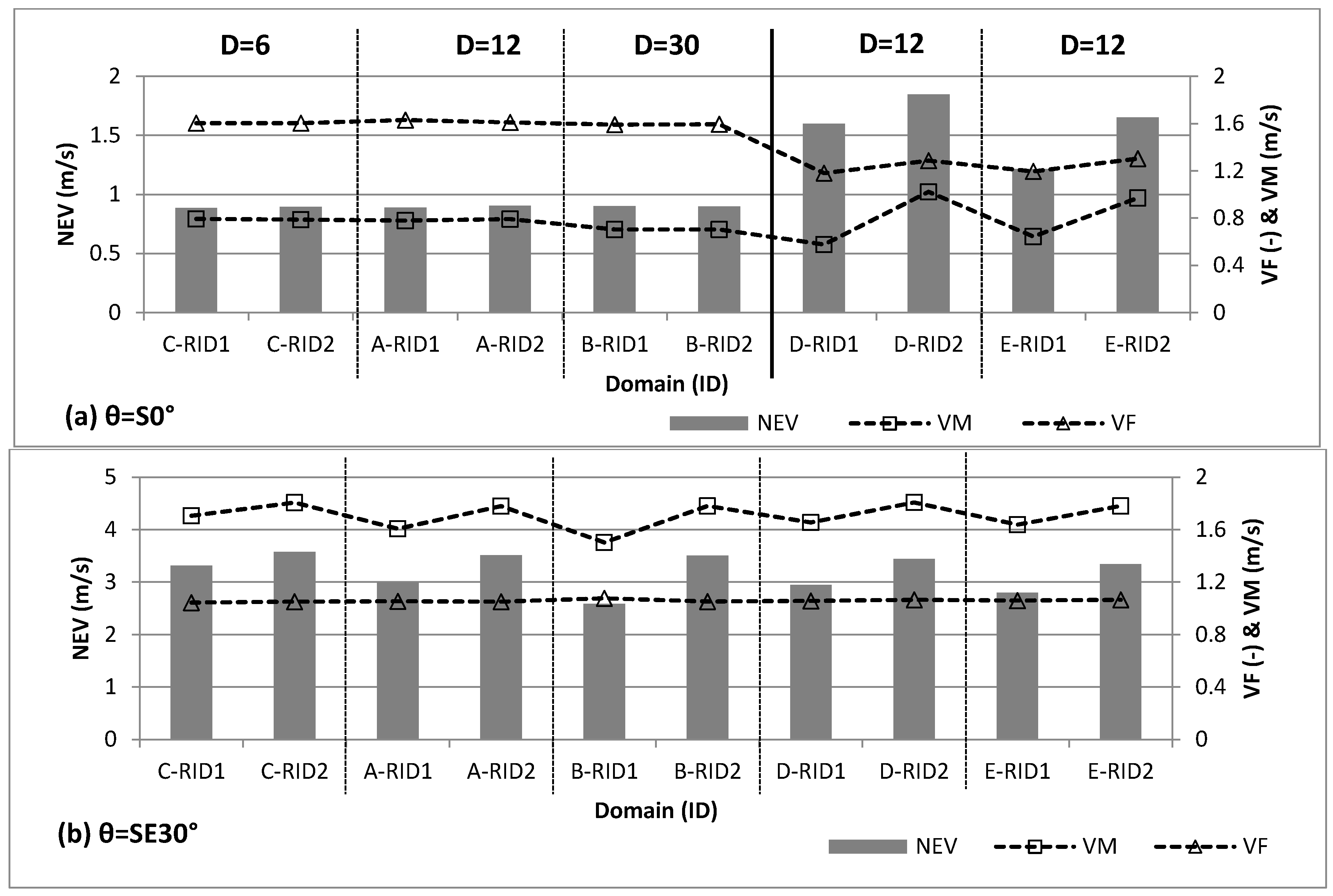
Figure 11 shows the concentration fields within RS space of different cases of building spacing and staggering, including changes under wind directions θ = S 0° and θ = SE 30°. Under the south 0° wind direction, pollutant concentrations in the RS space decreases slightly as building spacing D (D1 and D2) increases. However, this variation is not obvious, even when D increases to 30 m. The variation is mainly due to the effects of surrounding buildings. The building spacing of the south up-wind building is set at 12 m. Although D increases to 30 m, mean VM in space RS does not increase obviously, which leads to the limited improvement of pollutant dispersion. When the building arrangement is staggered, the level of pollutant concentration obviously increases. This increase is mainly due to the effect of staggered building arrangement, which blocks the air flow path in studied area. Figure 12a shows the influence of changes in building spacing and staggering on NEV, VM and VF of RS spaces. From the figure, it can be clearly observed that NEV generally decreases slightly as building spacing increases. When D = 12 (i.e., A-RS), NEV of the RS space in case A increases by approximately 65% from its value in case C (D = 6). This increase is mainly due to the increase of wind speed within the studied domain, as D increases under the aligned condition. However, when D increases to 30 m, mean VM of this studied domain does not increase. This failure to increase might be due to the effects of surrounding buildings, as discussed above. VF does increase slightly, so NEV of this domain decreases slightly. Under the staggered condition, it is clearly observed that the mean VM of this studied domain decreases, which induces the decrease of VE in the domain (35–60% decrease of NEV).
Under the wind direction θ = SE 30°, as the building length increases, the level of pollutant concentration in the study domains increases as D increases (Figure 11b). This is mainly due to the volume increase in the studied domain (increase in amount of pollutant released) and the limited improvement in ventilation efficiency. In Figure 12b, it can be observed that as D increases, although mean VM increases, VF also increases; and under the combined effect, NEV decreases slightly, which means the decreases of ventilation efficiency in this space.
7.3. Effect of Design Change in Outward-Side Space ROD
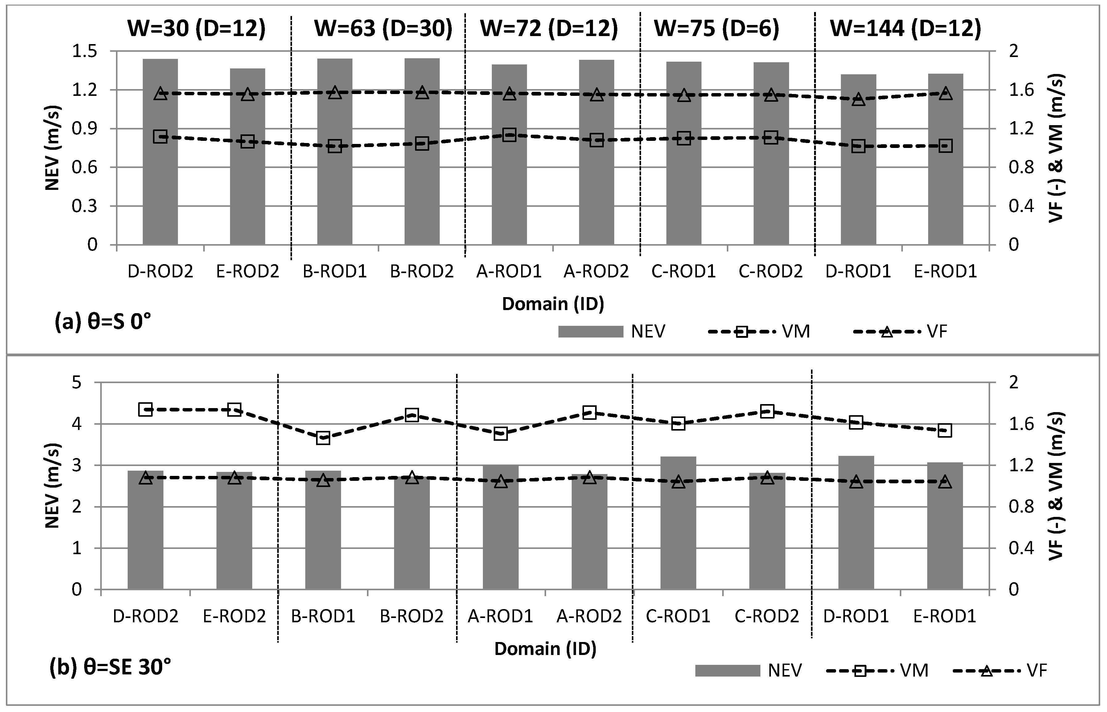
For the ROD space, these design variations nearly have negligible effect on spatial ventilation. Figure 13 shows the concentration fields within the ROD space (ROD1 and ROD2) for different design changes under wind directions θ = S 0° and θ = SE 30°. From Figure 13a, it can be observed that the level of pollutants within the domains show similar distribution patterns under the south 0° wind direction. This is mainly because the wind flow patterns within the studied domains are mainly influenced by the streets (St1 and St2) beside the space. As the street width does not change, air flow pattern in the studied domain does not change very much. Figure 14a shows the effects of design variations on VE indices within the ROD spaces. From this figure, it is obvious that VF, VM and their related NEV all do not change very much for different design cases. The change range is below 10%.
Under southeast 30° wind direction, distribution of pollutants within ROD2 domains is much less uniform than that of the ROD1 domains, and in some parts, the level of pollutants in the ROD2 domains is much higher (Figure 13b). The cause is similar to that in RM spaces. As the wind direction is from southeast, recirculation of flows within the ROD2 domains is more prominent than that of the RM1 domains, which induce the pollutants gathering in parts close to the buildings’ corners. In Figure 14b, it can also be seen that NEVs within the ROD2 domains are slightly higher than that of the RM1 domains.
7.4. Effect of Design Change in Inward-Side Space RID
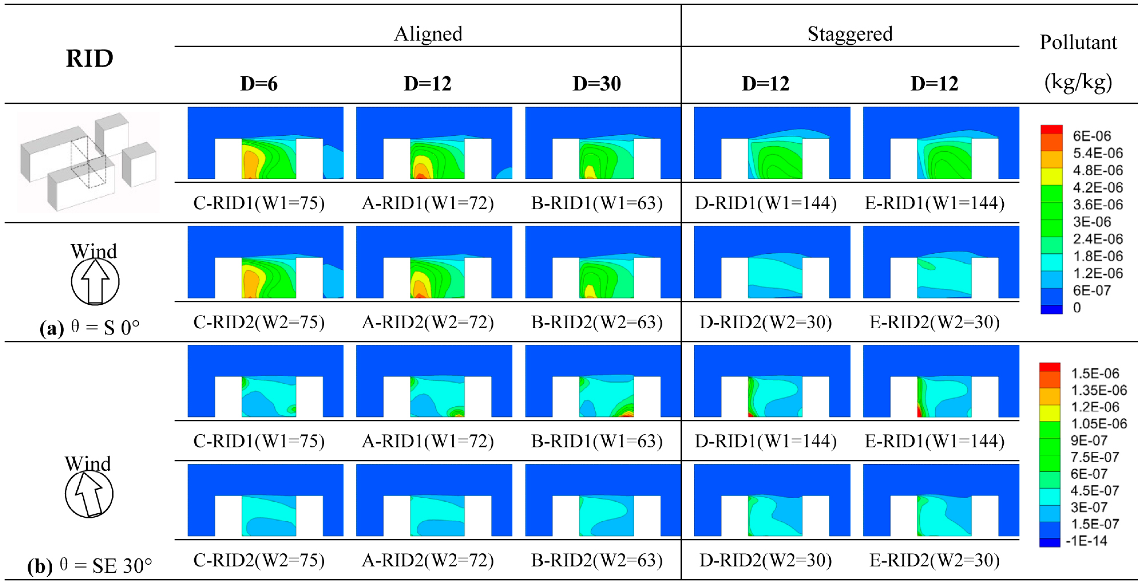
Figure 15 shows the concentration fields within the RID space of different cases under wind directions θ = S 0° and θ = SE 30°. In Figure 15a, it can be observed that, under south 0° wind direction, pollutant concentrations in Case D and Case E are evidently less than that in Case A, Case B and Case C. It is mainly due to the decrease of building length. In case D and Case E, when building length W2 is 30 m, the RID space is close to streets St1. The air flow pattern improves evidently, which can be seen in Figure 16a. In case D and Case E, VF decreases in all the RID spaces and VM even increase in the RID2 spaces. These flow characteristics induce that the value of NEV increase greatly. Moreover, in Case A, Case B and Case C, pollutant concentrations evidently decrease as building spacing D increases. This is mainly due to the increase in pollutant dispersion in the RID space, which is closely related to the air exchange rate. However, from Figure 16a, it can be observed that under these wind conditions, increase of NEV is limited, which means that pollutant spreading speed does not improve greatly as building spacing widens. This variation is coincident with that of spatial VM and VF. As building spacing increases, VM does not improve evidently, and VF decreases slightly. With these combined effects, NEV is slightly improved. This is mainly due to the effect of up-wind surrounding buildings.
Under the southeast 30° wind direction, wider building spacing might decrease the RID space’s VE. In Figure 15b, it can be observed that pollutant concentration in the RID1 space increases as building spacing D increases. This is mainly due to the effect of recirculation of flows, similar to the ROD space discussed above. However, under this wind direction, variation in building spacing has a nearly negligible effect on pollutant concentration of the RID2 space. The variation range of NEV in these spaces is below 2% (Figure 16b).
8. Conclusions
This study presents a preliminary investigation of the relevance of ventilation efficiency in outdoor space to various spatial patterns of residential buildings with the aid of CFD simulation techniques and the possibility of optimization through simulations at different spaces in typical cases. NEV, VM and VF were used to quantify the contributions of pollutant removal by mean flow and turbulent diffusion, as well as their ventilation capacities.
The simulation results indicate that NEV is a useful ventilation efficiency index that can comprehensively reflect the pollutant removal ability of wind velocity and flow recirculation in different regional spaces. VM and VF are also useful indicators that can reflect the influence on pollutant removal of wind velocity and flow recirculation, respectively. By combined applying these three indices, regional spatial ventilation performance can be effectively assessed.
From the cases studies, it can be determined that spatial patterns can strongly influence a space’s ventilation efficiency, especially when wind direction is approximately perpendicular to the main building facade. For residential building arrangements, strip-shaped buildings form a ventilation corridor between the southward-oriented buildings due to solar access demands. Thus, when wind direction changes from parallel to perpendicular along the building’s long facades, space ventilation generally decreases. In this study, when wind direction is perpendicular to buildings’ main facades, intersection space has the best ventilation efficiency, in general, due to the air-path, which leads to high VM and lower VF; the outward-side space shows relatively better ventilation efficiency due to wind inducing the air-path of streets (St1 and St2) beside the outward-side spaces. Ventilation efficiency of the inward-side spaces and middle spaces depend heavily on design variations in building length and spacing. For example, in case A, NEV of the middle space is 31% higher than that of inward-side space, which means ventilation efficiency of the middle space is better than that of the inward-side space, but when building length increases, NEV of the middle space in case D is 14% lower than that of the inward-side space in case A.
Through preliminary analysis of the influence of design variation on ventilation efficiency of different spaces, it can be observed that building spacing evidently influences ventilation performance of the inward-side space and intersection space. As building spacing increases, ventilation efficiency of these spaces improves evidently, but the improvement is restricted greatly by the effect of up-wind surrounding buildings. Variation in building length mainly has a great influence on ventilation performance of the middle spaces. As building length increases, ventilation efficiency of the middle spaces decreases. When building length becomes very long (i.e., 144 m in Case D), NEV of the middle spaces can decrease by about 50% due to decreased wind velocity in this domain.
Thus, it can be concluded that local prevailing wind direction should be considered in design operations specifically dealing with building orientation; consideration of wind direction is especially important for residential building arrangements. When a certain degree (i.e., 30°) exists between prevailing wind direction and building’s long facade, all ventilation efficiency indices can show sizable improvements in different regional spaces. Existing case studies show that building length, lateral spacing and staggered positioning can influence on ventilation efficiency of regional spaces. However, building length change is more relevant to outdoor ventilation of RM spaces, and residential buildings should be restricted to eight-living-unit combinations of dwellings. This might lead to more wind flow into the middle spaces, which can be beneficial for the middle living units. Lateral spacing and staggered positioning might have more of an effect on the intersection space and inward-side spaces. However, when considering lateral spacing and staggered design, surrounding building arrangements in the prevailing up-wind direction should be considered to organize air flow path, which could be beneficial for ventilation performance in these spaces.
This paper discusses the method of evaluating regional spatial ventilation performance for architects to improve residential building arrangements design. As a preliminary analysis of the relevance of spatial patterns to the wind environment in the city, this study uses a rather limited quantity and typology of spatial patterns and calculated data, which indicates a preliminary trend of variation in the influence of spatial patterns. Therefore, the need for more concrete and accurate evidence calls for further studies in the future.
Supplementary Materials
Supplementary materials can be found at www.mdpi.com/2073-4433/8/6/102/s1, Figure S1: Position P1, P2 and P3 of vertical line and central street line located in Case A, Figure S2: The wind velocity profiles along a vertical line at (a) position P1, (b) position P2, (c) position P3, (d) Distribution of wind velocity along the central street line (z = 0.1 H), Figure S3: Building configurations and arrangements (H = 18 m, W = 9 m, L1 = 48 m, L2 = 24 m), Figure S4: (a) Computational domain, Figure S5: Gird resolution in the computational domain, Table S1: The calculation conditions utilized in CFD simulation, Figure S6: Comparison of the numerical and experimental results at (a) position P1, (b) position P2, (c) position P3.
Acknowledgments
This study was financially supported by the National Natural Science Foundation of China (Grant No. 51508262 and No. 51538005).
Author Contributions
Wei You, Zhi Gao and Wowo Ding conceived and designed the experiments; Wei You performed the experiments and acquired the data; Wei You, Zhi Gao and Zhi Chen analyzed the data; and Wei You wrote the paper.
Conflicts of Interest
The authors declare no conflict of interest.
References
- Erell, E.; Pearlmutter, D.; Williamson, T. Urban Microclimate: Designing the Spaces between Buildings; Earthsan: Oxon, UK; New York, NY, USA, 2011. [Google Scholar]
- Givoni, B. Climate Considerations in Building and Urban Design; John Wiley & Sons: New York, NY, USA, 1998. [Google Scholar]
- Shi, X.; Zhu, Y.; Duan, J.; Shao, R.; Wang, J. Assessment of pedestrian wind environment in urban planning design. Landsc. Urban Plan. 2015, 140, 17–28. [Google Scholar] [CrossRef]
- Mfula, A.M.; Kukadia, V.; Griffithsa, R.F.; Hall, D.J. Wind tunnel modelling of urban building exposure to outdoor pollution. Atmos. Environ. 2005, 39, 2737–2745. [Google Scholar] [CrossRef]
- Chen, L.; Hang, J.; Sandberg, M.; Claesson, L.; Di Sabatino, S.; Wigo, H. The impacts of building height variations and building packing densities on flow adjustment and city breathability in idealized urban models. Build. Environ. 2017, 118, 344–361. [Google Scholar] [CrossRef]
- Simöens, S.; Ayraulta, M.; Wallace, J.M. The flow across a street canyon of variable width—Part 1: Kinematic description. Atmos. Environ. 2007, 41, 9002–9017. [Google Scholar] [CrossRef]
- Simöens, S.; Wallace, J.M. The flow across a street canyon of variable width—Part 2: Scalar dispersion from a street level line source. Atmos. Environ. 2008, 42, 2489–2503. [Google Scholar] [CrossRef]
- Dong, J.; Tan, Z.; Xiao, Y.; Tu, J. Seasonal Changing Effect on Airflow and Pollutant Dispersion Characteristics in Urban Street Canyons. Atmosphere 2017, 8, 43. [Google Scholar] [CrossRef]
- Tsang, C.W.; Kwok, K.C.; Hitchcock, P.A. Wind tunnel study of pedestrian level wind environment around tall buildings: Effects of building dimensions, separation and podium. Build. Environ. 2012, 49, 167–181. [Google Scholar] [CrossRef]
- Hong, B.; Lin, B. Numerical studies of the outdoor wind environment and thermal comfort at pedestrian level in housing blocks with different building layout patterns and trees arrangement. Renew. Energy 2015, 73, 18–27. [Google Scholar] [CrossRef]
- Yang, F.; Gao, Y.; Zhong, K.; Kang, Y. Impacts of cross-ventilation on the air quality in street canyons with different building arrangements. Build. Environ. 2016, 104, 1–12. [Google Scholar] [CrossRef]
- Ng, W.Y.; Chau, C.K. A modeling investigation of the impact of street and building configurations on personal air pollutant exposure in isolated deep urban canyons. Sci. Total Environ. 2014, 468, 429–448. [Google Scholar] [CrossRef] [PubMed]
- Bady, M.; Katob, K.; Huang, H. Towards the application of indoor ventilation efficiency indices to evaluate the air quality of urban areas. Build. Environ. 2008, 43, 1991–2004. [Google Scholar] [CrossRef]
- Kato, K.; Huang, H. Ventilation efficiency of void space surrounded by buildings with wind blowing over built-up urban area. J. Wind Eng. Ind. Aerodyn. 2009, 97, 358–367. [Google Scholar] [CrossRef]
- Buccolieri, R.; Sandberg, M.; Di Sabatino, D. City breathability and its link to pollutant concentration distribution within urban-like geometries. Atmos. Environ. 2010, 44, 1894–1903. [Google Scholar] [CrossRef]
- Hang, J.; Sandberg, M.; Li, Y. Age of air and air exchange efficiency in idealized city models. Build. Environ. 2009, 44, 1714–1723. [Google Scholar] [CrossRef]
- Hang, J.; Wang, Q.; Chen, X.; Sandberg, M.; Zhu, W.; Buccolieri, R.; Di Sabatino, S. City breathability in medium density urban-like geometries evaluated through the pollutant transport rate and the net escape velocity. Build. Environ. 2015, 94, 166–182. [Google Scholar] [CrossRef]
- You, W.; Ding, W.W. Assessment of outdoor space’s ventilation efficiency around residential building: Effects of building dimension, separation and orientation. Proceedings of 50th International Conference of the Architectural Science Association (ASA), The University of Adelaide, Adelaide, Australia, 7–9 December 2016; pp. 219–228. [Google Scholar]
- Buccolieri, R.; Salizzoni, P.; Soulhac, L.; Garbero, V.; Di Sabatino, S. The breathability of compact cities. Urban Clim. 2015, 13, 73–93. [Google Scholar] [CrossRef]
- Di Sabatino, S.; Buccolieri, R.; Pulvirenti, B.; Britter, R. Simulations of pollutant dispersion within idealized urban-type geometries with CFD and integral models. Atmos. Environ. 2007, 41, 8316–8329. [Google Scholar] [CrossRef]
- Hang, J.; Li, Y. Age of air and air exchange efficiency in high-rise urban areas and its link to pollutant dilution. Atmos. Environ. 2011, 45, 5572–5585. [Google Scholar]
- Hang, J.; Li, Y.; Sandberg, M.; Buccolieri, R.; di Sabatino, S. The influence of building height variability on pollutant dispersion and pedestrian ventilation in idealized high-rise urban areas. Build. Environ. 2012, 56, 346–360. [Google Scholar] [CrossRef]
- Lin, M.; Hang, J.; Li, Y.; Luo, Z.; Sandberg, M. Quantitative ventilation assessments of idealized urban canopy layers with various urban layouts and the same building packing density. Build. Environ. 2014, 79, 152–167. [Google Scholar]
- Ramponi, R.; Blocken, B.; Laura, B.; Janssen, W.D. CFD simulation of outdoor ventilation of generic urban configurations with different urban densities and equal and unequal street widths. Build. Environ. 2015, 92, 152–166. [Google Scholar] [CrossRef]
- Razak, A.A.; Hagishima, A.; Ikegaya, N.; Tanimoto, J. Analysis of airflow over building arrays for assessment of urban wind environment. Build. Environ. 2013, 59, 56–65. [Google Scholar] [CrossRef]
- Lee, R.X.; Jusuf, S.K.; Wong, N.H. The study of height variation on outdoor ventilation for Singapore’s high-rise residential housing estates. Int. J. Low-Carbon Technol. 2015, 10, 15–33. [Google Scholar] [CrossRef]
- Oke, T.R. Street Design and Urban Canopy Layer Climate. Energy Build. 1988, 11, 103–113. [Google Scholar] [CrossRef]
- Sini, J.F.; Anquetin, S.; Mestayer, P.G. Pollutant dispersion and thermal effects in urban street canyons. Atmos. Environ. 1996, 30, 2659–2677. [Google Scholar] [CrossRef]
- Chan, A.T.; So, E.S.; Samad, S.C. Strategic guidelines for street canyon geometry to achieve sustainable street air quality. Atmos. Environ. 2001, 35, 4089–4098. [Google Scholar] [CrossRef]
- Chan, A.T.; Au, W.T.; So, E.S. Strategic guidelines for street canyon geometry to achieve sustainable street air quality—Part II: Multiple canopies and canyons. Atmos. Environ. 2003, 37, 2761–2772. [Google Scholar] [CrossRef]
- Ying, X.; Zhu, W.; Hokao, K.; Ge, J. Numerical research of layout effect on wind environment around high-rise buildings. Archit. Sci. Rev. 2013, 56, 272–278. [Google Scholar] [CrossRef]
- Iqbal, Q.M.Z.; Chan, A.L.S. Pedestrian level wind environment assessment around group of high-rise cross-shaped buildings: Effect of building shape, separation and orientation. Build. Environ. 2016, 101, 45–63. [Google Scholar] [CrossRef]
- Blocken, B. 50 years of Computational Wind Engineering: Past, present and future. J. Wind Eng. Ind. Aerodyn. 2014, 129, 69–102. [Google Scholar] [CrossRef]
- Stathopoulos, T. Computational wind engineering: Past achievements and future challenges. J. Wind Eng. Ind. Aerodyn. 1997, 67, 509–532. [Google Scholar] [CrossRef]
- Blocken, B.; Stathopoulos, T.; Carmeliet, J.; Hensen, J.L. Application of computational fluid dynamics in building performance simulation for the outdoor environment: An overview. J. Build. Perform. Simul. 2011, 4, 157–184. [Google Scholar] [CrossRef]
- Stathopoulos, T. Pedestrian level winds and outdoor human comfort. J. Wind Eng. Ind. Aerodyn. 2006, 94, 769–780. [Google Scholar] [CrossRef]
- Moonen, P.; Defraeye, T.; Dorer, V.; Blocken, B.; Carmeliet, J. Urban Physics: Effect of the micro-climate on comfort, health and energy demand. Front. Archit. Res. 2012, 1, 197–228. [Google Scholar] [CrossRef]
- Blocken, B.; Stathopoulos, T.; Van Beeck, J.P.A.J. Pedestrian-level wind conditions around buildings: Review of wind-tunnel and CFD techniques and their accuracy for wind comfort assessment. Build. Environ. 2016, 100, 50–81. [Google Scholar] [CrossRef]
- Blocken, B. Computational Fluid Dynamics for urban physics: Importance, scales, possibilities, limitations and ten tips and tricks towards accurate and reliable simulations. Build. Environ. 2015, 91, 219–245. [Google Scholar] [CrossRef]
- Tominaga, Y.; Mochida, A.; Yoshie, R.; Kataoka, H.; Nozue, T.; Yoshikawa, M.; Shirasawa, T. AIJ guidelines for practical applications of CFD to pedestrian wind environment around buildings. J. Wind Eng. Ind. Aerodyn. 2008, 96, 1749–1761. [Google Scholar] [CrossRef]
- Franke, J.; Hellsten, A.; Schlünzen, K.H.; Carissimo, B. The COST 732 Best Practice Guideline for CFD simulation of flows in the urban environment: A summary. Int. J. Environ. Pollut. 2011, 44, 419–427. [Google Scholar] [CrossRef]
- Yuan, C.; Ng, E. Building porosity for better urban ventilation in high-density cities—A computational parametric study. Build. Environ. 2012, 50, 176–189. [Google Scholar] [CrossRef]
- Yuan, C.; Ng, E.; Norford, L.K. Improving air quality in high-density cities by understanding the relationship between air pollutant dispersion and urban morphologies. Build. Environ. 2014, 71, 245–258. [Google Scholar] [CrossRef]
- Ng, E.; Yuan, C.; Chen, L.; Ren, C.; Fung, J.C. Improving the wind environment in high-density cities by understanding urban morphology and surface roughness: A study in Hong Kong. Landsc. Urban Plan. 2011, 101, 59–74. [Google Scholar] [CrossRef]
- Wong, M.S.; Nichol, J.; Ng, E. A study of the “wall effect” caused by proliferation of high-rise buildings using GIS techniques. Landsc. Urban Plan. 2011, 102, 245–253. [Google Scholar] [CrossRef]
- Yuan, C.; Ng, E. Practical application of CFD on environmentally sensitive architectural design at high density cities: A case study in Hong Kong. Urban Clim. 2014, 8, 57–77. [Google Scholar] [CrossRef]
- Ng, E. Policies and technical guidelines for urban planning of high-density cities—Air ventilation assessment (AVA) of Hong Kong. Build. Environ. 2009, 44, 1478–1488. [Google Scholar] [CrossRef]
- Kubota, T.; Miura, M.; Tominaga, Y.; Mochid, A. Wind tunnel tests on the relationship between building density and pedestrian-level wind velocity: Development of guidelines for realizing acceptable wind environment in residential neighborhoods. Build. Environ. 2008, 43, 1699–1708. [Google Scholar] [CrossRef]
- Liu, Q.; Ding, W. Morphological study on units of Fabric that constitute contemporary residential plot in the Yangtze River Delta, China. In Proceedings of the 19th International Seminar on Urban Form (ISUF), Delft, The Netherlands, 16–19 October 2012; pp. 689–694. [Google Scholar]
- Zhao, Q.; Ding, W. Relevance study: Relationship of morphological characteristics between residential plot and building pattern in Nanjing, China. In Proceedings of the 21th International Seminar on Urban Form (ISUF), Porto, Portugal, 3–6 July 2014. [Google Scholar]
- Franke, J.; Hellsten, A.; Schlünzen, H.; Carissimo, B. Best Practice Guideline for the CFD Simulation of Flows in the Urban Environment; COST Office: Brussels, Belgium, 2007; ISBN 3-00-018312-4. [Google Scholar]
- Tominag, Y.; Stathopoulos, T. Numerical simulation of dispersion around an isolated cubic building: Model evaluation of RANS and LES. Build. Environ. 2010, 45, 2231–2239. [Google Scholar] [CrossRef]
- Blocken, B.; van der Hout, A.; Dekker, J.; Weiler, O. CFD simulation of wind flow over natural complex terrain: Case study with validation by field measurements for Ria de Ferrol, Galicia, Spain. J. Wind Eng. Ind. Aerodyn. 2015, 147, 905–928. [Google Scholar] [CrossRef]
- Tominaga, Y.; Mochida, A.; Shirasawa, T.; Yoshie, R.; Kataoka, H.; Harimoto, K.; Nozu, T. Cross Comparisons of CFD Results of Wind Environment at Pedestrian Level around a high-rise Building and within a Building Complex. J. Asian Archit. Build. Eng. 2004, 3, 63–70. [Google Scholar] [CrossRef]
- Zhang, A.; Gao, C.; Zhang, L. Numerical simulation of the wind field around different building arrangements. J. Wind Eng. Ind. Aerodyn. 2005, 93, 891–904. [Google Scholar] [CrossRef]
- Lim, E.; Ito, K.; Sandberg, M. New ventilation index for evaluating imperfect mixing conditions—Analysis of Net Escape Velocity based on RANS approach. Build. Environ. 2013, 61, 45–56. [Google Scholar] [CrossRef]
Figure 1.
View of typical residential building arrangements in China: (a) Shenzhen; (b) Nanjing; (c) Shanghai; and (d) Beijing.
Figure 1.
View of typical residential building arrangements in China: (a) Shenzhen; (b) Nanjing; (c) Shanghai; and (d) Beijing.
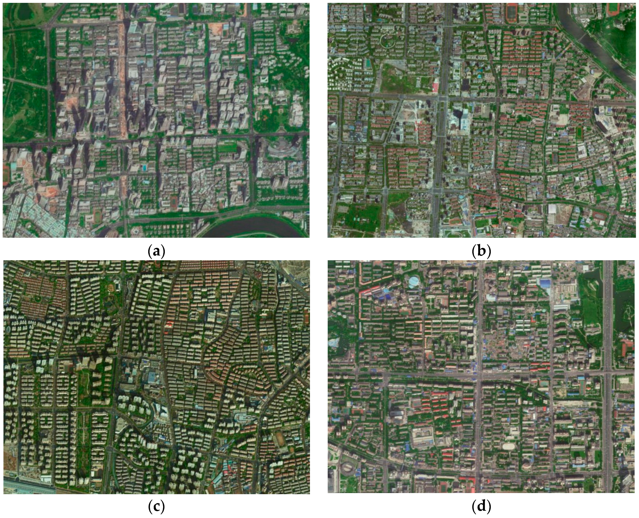
Figure 2.
Living units and unit combination in a residential building: (a) Residential building size; (b) Living unit types (unit: m); (c) Living unit combination.
Figure 2.
Living units and unit combination in a residential building: (a) Residential building size; (b) Living unit types (unit: m); (c) Living unit combination.
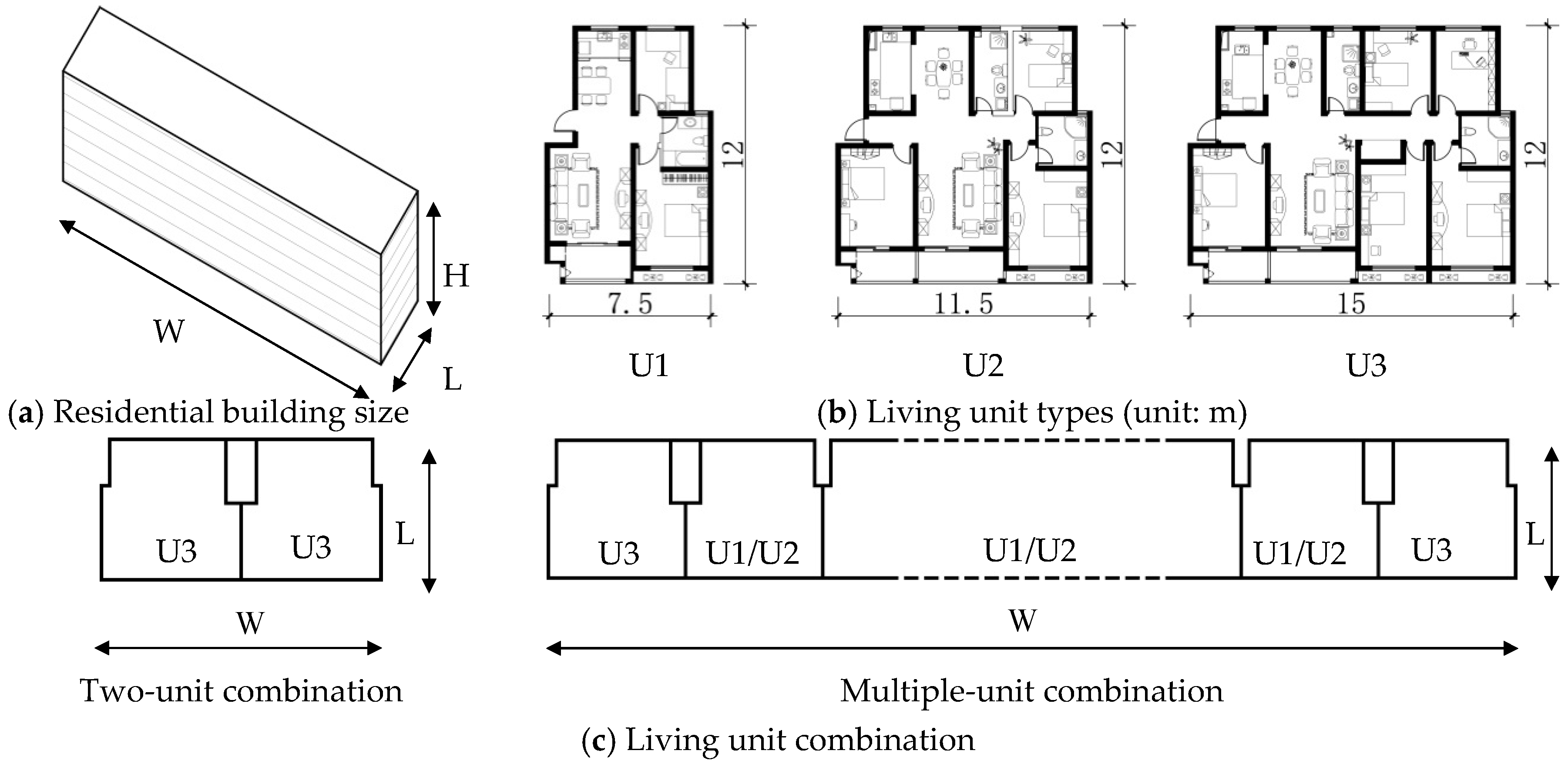
Figure 3.
Setup of calculation cases (Units m): (a) Calculated residential building model (B1 = 24, B2 = D3 = 30); (b) Building layout patterns.
Figure 3.
Setup of calculation cases (Units m): (a) Calculated residential building model (B1 = 24, B2 = D3 = 30); (b) Building layout patterns.

Figure 4.
Typical studied areas and space pattern classification (Unit: m): (a) Studied domain; (b) Space pattern classification of studied domain.
Figure 4.
Typical studied areas and space pattern classification (Unit: m): (a) Studied domain; (b) Space pattern classification of studied domain.
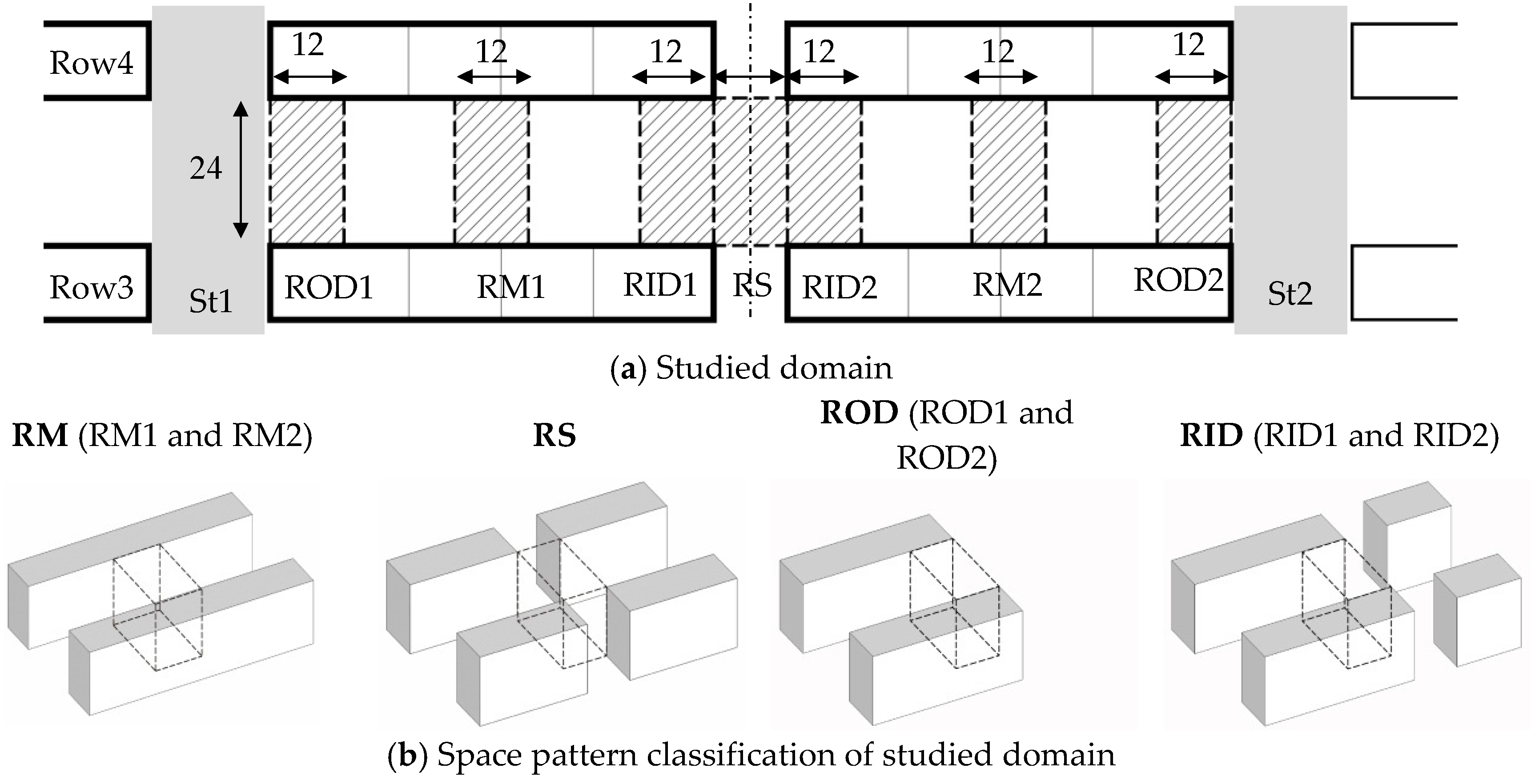
Figure 5.
Computational domain and boundary conditions.

Figure 6.
Gird resolution in the computational domain (Case A).
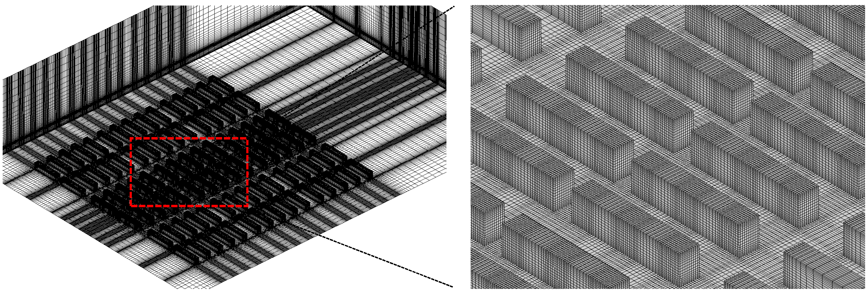
Figure 7.
Wind flow patterns for five cases under two wind directions (θ = S 0° and θ = SE 30°) and studied domains for each case (z = 0.1 H).
Figure 7.
Wind flow patterns for five cases under two wind directions (θ = S 0° and θ = SE 30°) and studied domains for each case (z = 0.1 H).

Figure 8.
Ventilation performance of different studied domains for five cases under wind direction: (a) θ = S 0°; and (b) θ = SE 30°.
Figure 8.
Ventilation performance of different studied domains for five cases under wind direction: (a) θ = S 0°; and (b) θ = SE 30°.

Figure 9.
Concentration fields within the studied RM1 and RM2 domains (RM space) for different design variations under wind direction: (a) θ = S 0°; and (b) θ = SE 30° (Unit: m).
Figure 9.
Concentration fields within the studied RM1 and RM2 domains (RM space) for different design variations under wind direction: (a) θ = S 0°; and (b) θ = SE 30° (Unit: m).

Figure 10.
Effect of building length on ventilation efficiency indices within RM1 and RM2 domains (RM space) under wind direction: (a) θ = S 0°; and (b) θ = SE 30° (Unit: m).
Figure 10.
Effect of building length on ventilation efficiency indices within RM1 and RM2 domains (RM space) under wind direction: (a) θ = S 0°; and (b) θ = SE 30° (Unit: m).

Figure 11.
Concentration fields within studied RS space for different arrangements and building spacing under wind direction: (a) θ = S 0°; and (b) θ = SE 30° (Unit: m).
Figure 11.
Concentration fields within studied RS space for different arrangements and building spacing under wind direction: (a) θ = S 0°; and (b) θ = SE 30° (Unit: m).

Figure 12.
Effect of building spacing on ventilation efficiency indices within the RS space under wind direction: (a) θ = S 0°; and (b) θ = SE 30° (Unit: m).
Figure 12.
Effect of building spacing on ventilation efficiency indices within the RS space under wind direction: (a) θ = S 0°; and (b) θ = SE 30° (Unit: m).

Figure 13.
Concentration fields within studied ROD1 and ROD2 domains (ROD space) for different design variations under wind direction: (a) θ = S 0°; and (b) θ = SE 30° (Unit: m).
Figure 13.
Concentration fields within studied ROD1 and ROD2 domains (ROD space) for different design variations under wind direction: (a) θ = S 0°; and (b) θ = SE 30° (Unit: m).
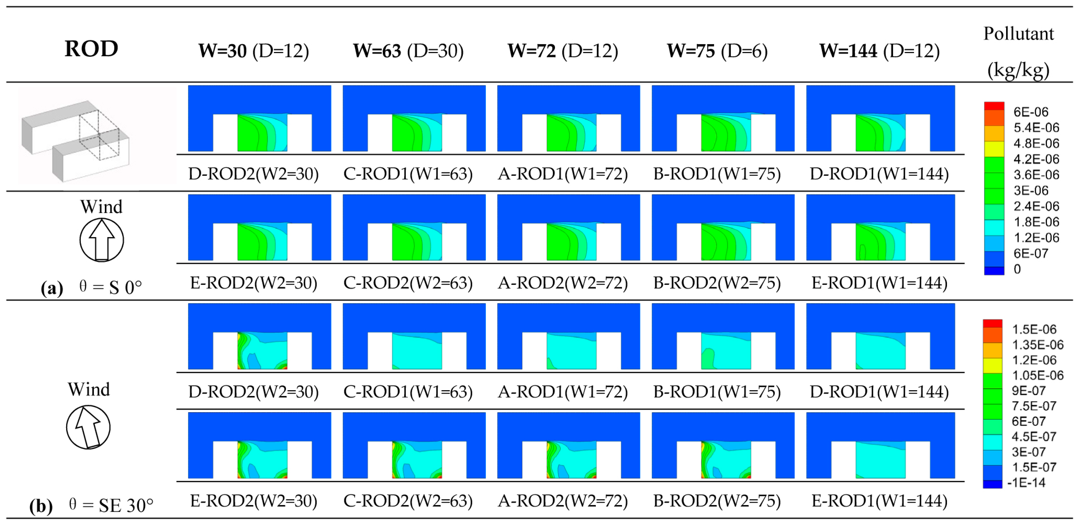
Figure 14.
Effect of design variations on ventilation efficiency indices within ROD1 and ROD2 domains (ROD space) under wind direction: (a) θ = S 0°; and (b) θ = SE 30° (Unit: m).
Figure 14.
Effect of design variations on ventilation efficiency indices within ROD1 and ROD2 domains (ROD space) under wind direction: (a) θ = S 0°; and (b) θ = SE 30° (Unit: m).

Figure 15.
Concentration fields within the studied RID1 and RID2 domains (RID space) for different design variations under wind direction: (a) θ = S 0°; and (b) θ = SE 30° (unit: m).
Figure 15.
Concentration fields within the studied RID1 and RID2 domains (RID space) for different design variations under wind direction: (a) θ = S 0°; and (b) θ = SE 30° (unit: m).

Figure 16.
Effect of design variations on ventilation efficiency indices within the RID1 and RID2 domains (RID space) under wind direction: (a) θ = S 0°; and (b) θ = SE 30° (unit: m).
Figure 16.
Effect of design variations on ventilation efficiency indices within the RID1 and RID2 domains (RID space) under wind direction: (a) θ = S 0°; and (b) θ = SE 30° (unit: m).

© 2017 by the authors. Licensee MDPI, Basel, Switzerland. This article is an open access article distributed under the terms and conditions of the Creative Commons Attribution (CC BY) license (http://creativecommons.org/licenses/by/4.0/).
Share and Cite
MDPI and ACS Style
You, W.; Gao, Z.; Chen, Z.; Ding, W. Improving Residential Wind Environments by Understanding the Relationship between Building Arrangements and Outdoor Regional Ventilation. Atmosphere 2017, 8, 102. https://doi.org/10.3390/atmos8060102
AMA Style
You W, Gao Z, Chen Z, Ding W. Improving Residential Wind Environments by Understanding the Relationship between Building Arrangements and Outdoor Regional Ventilation. Atmosphere. 2017; 8(6):102. https://doi.org/10.3390/atmos8060102
Chicago/Turabian StyleYou, Wei, Zhi Gao, Zhi Chen, and Wowo Ding. 2017. "Improving Residential Wind Environments by Understanding the Relationship between Building Arrangements and Outdoor Regional Ventilation" Atmosphere 8, no. 6: 102. https://doi.org/10.3390/atmos8060102
Note that from the first issue of 2016, this journal uses article numbers instead of page numbers. See further details here.