Effects of Boundary Layer Height on the Model of Ground-Level PM_2.5 Concentrations from AOD: Comparison of Stable and Convective Boundary Layer Heights from Different Methods

Abstract

The aerosol optical depth (AOD) from satellites or ground-based sun photometer spectral observations has been widely used to estimate ground-level PM_2.5 concentrations by regression methods. The boundary layer height (BLH) is a popular factor in the regression model of AOD and PM_2.5, but its effect is often uncertain. This may result from the structures between the stable and convective BLHs and from the calculation methods of the BLH. In this study, the boundary layer is divided into two types of stable and convective boundary layer, and the BLH is calculated using different methods from radiosonde data and National Centers for Environmental Prediction (NCEP) reanalysis data for the station in Beijing, China during 2014–2015. The BLH values from these methods show significant differences for both the stable and convective boundary layer. Then, these BLHs were introduced into the regression model of AOD-PM_2.5 to seek the respective optimal BLH for the two types of boundary layer. It was found that the optimal BLH for the stable boundary layer is determined using the method of surface-based inversion, and the optimal BLH for the convective layer is determined using the method of elevated inversion. Finally, the optimal BLH and other meteorological parameters were combined to predict the PM_2.5 concentrations using the stepwise regression method. The results indicate that for the stable boundary layer, the optimal stepwise regression model includes the factors of surface relative humidity, BLH, and surface temperature. These three factors can significantly enhance the prediction accuracy of ground-level PM_2.5 concentrations, with an increase of determination coefficient from 0.50 to 0.68. For the convective boundary layer, however, the optimal stepwise regression model includes the factors of BLH and surface wind speed. These two factors improve the determination coefficient, with a relatively low increase from 0.65 to 0.70. It is found that the regression coefficients of the BLH are positive and negative in the stable and convective regression models, respectively. Moreover, the effects of meteorological factors are indeed related to the types of BLHs.

1. Introduction

Air pollution seriously affects the environment and endangers human health. Smaller particles with aerodynamic diameters less than 2.5 µm (also known as PM_2.5) are dominant in industrial and urban pollution and can increase the incidence of heart disease, cardiovascular disease and lung cancer [1,2,3,4]. Most aerosols are emitted into the atmospheric boundary layer and result in serious pollution near the ground. However, the space coverage of PM_2.5 monitoring stations is sparse, especially in the suburban environment. Aerosol optical depth (AOD) data from satellites or ground-based sun photometer spectral observations can play an auxiliary role in air quality monitoring. AOD is the integral of the aerosol extinction due to scattering and absorption in the vertical plane, and surface PM_2.5 concentrations are related to the aerosol extinction. There is a wide body of literature that shows that there are strong correlations between AOD and surface PM_2.5 concentrations [5,6,7].

The regression method is widely employed for estimating ground-level PM_2.5 concentrations. Some meteorological parameters such as temperature, relative humidity, and wind are introduced into the regression model of AOD-PM_2.5 to improve the accuracy of estimating PM_2.5 concentrations [8,9,10]. Boundary layer height (BLH) is a popular parameter in the regression model, because it can indicate the height of turbulent diffusion. A higher BLH implies stronger turbulent diffusion, and usually results in a lower surface PM_2.5 concentration [11,12].

However, some studies have suggested that the effect of BLH is uncertain or insignificant to the regression model of AOD-PM_2.5 [8,13,14]. Tian and Chen [8] investigated the effects of the BLH and meteorological factors on the regression model of MODIS AOD in southern Ontario, Canada during 2004. They found that the P value of the BLH is 0.71, which is far larger than 0.01. It is suggested that the BLH is an ineffective factor for the regression model. Liu et al. [13] reported that the BLH is not significant at the α = 0.05 level in the model of Multiangle Imaging Spector Radiometer (MISR) AOD in the St Louis, Missouri, USA. One possible reason for the failure of the BLH in the model is that there are considerable calculation errors, especially for the BLH from the model product. Even using the radiosonde data, it is difficult to estimate an actual BLH, because the structure of the actual boundary layer is complex and varies with different definition and calculation methods [15].

Generally, the boundary layer is classified into the stable boundary layer and the convective boundary layer [16,17]. The stable boundary layer height is commonly defined as the height where the negative buoyancy flux at the surface damps the turbulence. It is always associated with a surface-based temperature inversion, and can be estimated by the top of the inversion using the temperature profile [18,19,20]. The convective boundary layer height is commonly defined as the height where the positive buoyancy flux at the surface creates a thermal instability. There are several methods to estimate convective BLH using the temperature, humidity, and refractivity profiles of sounding data, and the values of BLH calculated from these methods are usually different [17,21,22]. In addition, BLHs can also be estimated from a model, but the values depend on the model and its boundary layer parameterization. These differences may affect the application and assessment of BLH in the regression model of AOD-PM_2.5.

In this study, the BLHs calculated from radiosonde data and NCEP reanalysis data were compared for the station in Beijing, China during 2014–2015. Then, these BLHs were respectively introduced into the regression model to seek the optimal stable and convective BLHs. Finally, we used the optimal BLH and meteorological parameters to improve the prediction of ground-level PM_2.5 concentrations. In this paper, the materials and methodology are described in Section 2 and Section 3, respectively. A comparison of BLHs and their effect on the AOD-PM_2.5 regression equation are analyzed and discussed in Section 4. Several major conclusions and potential future improvements to the model of AOD-PM_2.5 are summarized in Section 5.

2. Materials

To assess the effects of BLHs in the regression model of AOD-PM_2.5, four types of data sets were collected, including hourly PM_2.5 concentrations, Aerosol Robotic Network (AERONET) AOD, NCEP reanalysis data, and radiosonde data. These data sets were collected in the Beijing area. However, the specific sites of stations for these data sets vary (Figure 1). The distances between the PM_2.5, AERONET, and radiosonde stations are less than 10 km, and the center resides at the AERONET station. The NCEP grid data were also interpolated with respect to the AERONET station. Section 2.1, Section 2.2, Section 2.3 and Section 2.4 describe each data set in more detail.

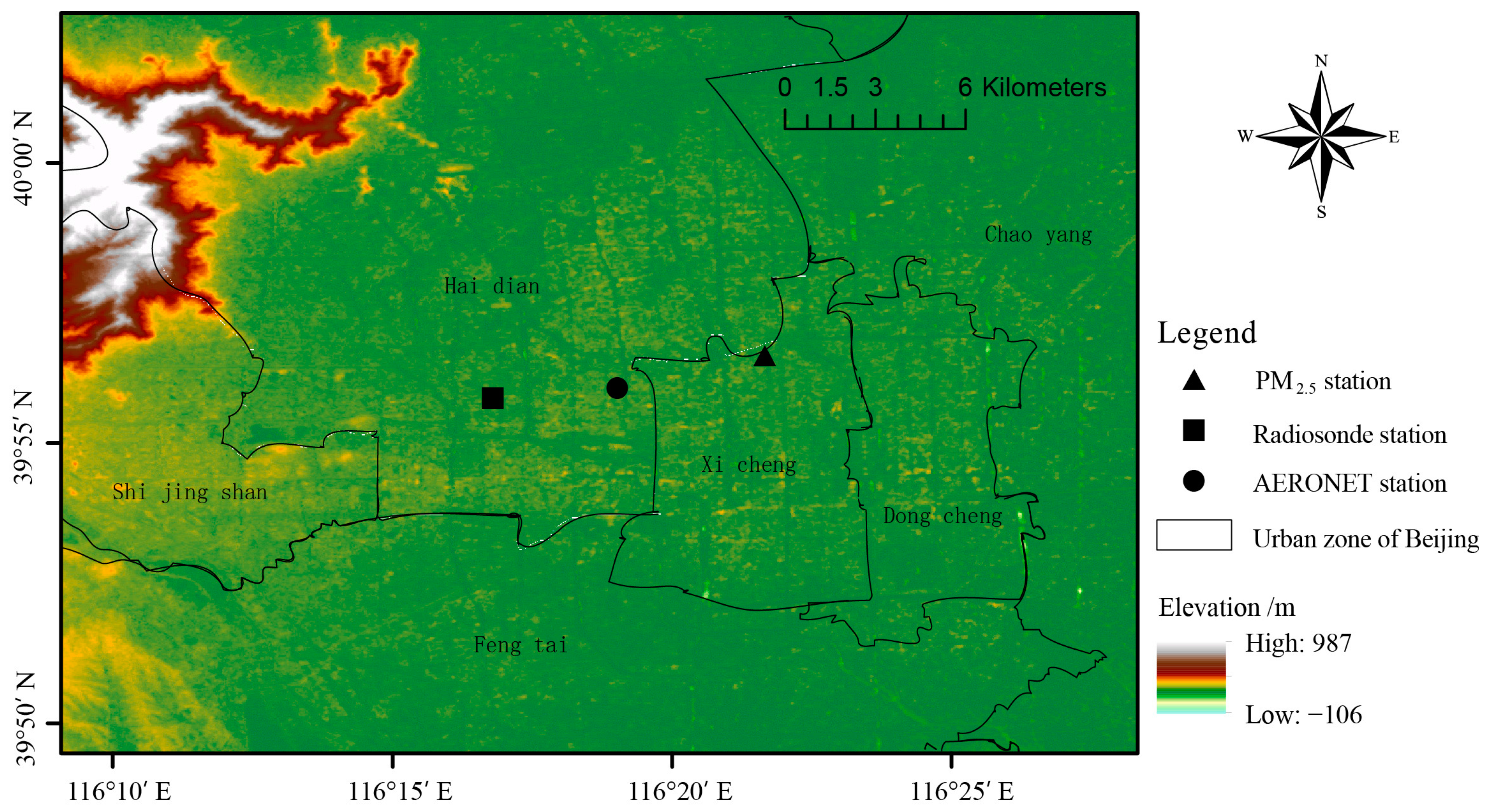
2.1. Radiosonde Data

The radiosonde measurements are obtained from the National Climate Data Center’s (NCDC) Integrated Global Radiosonde Archive (IGRA) [17,23]. The latest version of the NCDC IGRA provides quality-assured daily radiosonde records at mandatory pressure levels, additionally required levels, and thermodynamically significant levels [24,25]. The records of these levels can describe the detailed construction of the troposphere, and are widely used to calculate the BLH [18,20,26]. The radiosonde records consist of temperature, pressure, relative humidity, wind direction, and wind speed. Typically, radiosondes are launched two times per day at 00:00 UTC and 12:00 UTC. In this study, the radiosonde at 00:00 UTC from 1 January 2014 to 31 December 2015 were used and matched with other data.

2.2. Ground-Based PM_2.5 Concentration Data

The PM_2.5 concentration data are collected from the Ministry of Environmental Protection (MEP) of China. The concentration is measured hourly by a Tapered Element Oscillating Microbalance (TEOM) with an accuracy of 1.5 µg/m³. There are 12 PM_2.5 monitoring stations in the Beijing area. The Guan-Yuan station is the nearest PM_2.5 monitoring station to the radiosonde station, which is approximately 10 km away (Figure 1). Since the radiosonde is launched once per day at 00:00 UTC, the hourly PM_2.5 concentration at 00:00 UTC is selected. Invalid data (values recorded as NAN) because of equipment breakdown are removed.

2.3. AERONET AOD Data

The AERONET is a globally distributed network of sun photometers that provides multi-wavelength (340, 380, 440, 500, 675, 870, 940, and 1020 nm) AOD measurements [27,28,29]. The surface sun photometer employed by the AERONET has a very narrow field of view, and is therefore rarely affected by surface reflectance and aerosol forward scattering [30]. The AOD-retrieval uncertainty of AERONET AOD is only 0.01–0.02, and is widely used to validate satellite AOD values [31,32,33]. There are five AERONET stations in the Beijing area. The Beijing-CAMS AERONET station is located 5.0 km from the closest radiosonde station (Figure 1) and can provide a complete data record during 2014–2015. AERONET AOD data are computed for three data quality levels: level 1.0 (unscreened), level 1.5 (cloud-screened), and level 2.0 (cloud-screened and quality-assured). Data processing, cloud-screening algorithm, and inversion techniques are described by Holben et al. (1998, 2001). For the Beijing-CAMS station, only level 1.0 and level 1.5 data were available for the dates of interest. The data of level 1.5 are used widely in the previous studies [34,35,36]. In this study, we used the AERONET Level 1.5 (cloud-screened) aerosol product from the Beijing-CAMS station at a wavelength of 500 nm. The radiosonde is at 00:00 UTC, but the AERONET observations are usually not taken exactly at 00:00 UTC. There is a small interval of a few minutes near 00:00 UTC. The averaged AOD from 23:30 to 00:30 UTC was matched with the radiosonde at 00:00 UTC. In addition, if the standard deviation of the average AOD was greater than 0.5, the average AOD was removed to reduce the possibility of spurious AOD values [13,37].

2.4. BLH Data From NCEP

In addition to the BLH calculated from the sounding profile, we also used the BLH from the NCEP’s global reanalysis data, with a horizontal resolution of 1° × 1° and a time step of 6 h (00:00, 06:00, 12:00, and 18:00 UTC). The NCEP uses the bulk Richardson number (Ri) approach to iteratively estimate BLH starting from the ground upward [38,39]. This approach is suitable for both stable and convective boundary layers [26]. More detailed information of this reanalysis product can be found on the NOAA website [40]. In this study, only the 00:00 UTC BLH during 2014–2015 are collected. Note that the NCEP reanalysis data are on a regular latitude/longitude grid. The grid-cell BLHs were interpolated to the AERONET station using the inverse distance weighting method.

3. Methodology

3.1. The Method Used to Estimate the BLH

The BLH is divided into two types: the stable BLH and convective BLH. If there is a surface-based inversion in the sounding profile, the BLH is classified as the stable BLH (${\mathrm{BLH}}^{\mathrm{Sta}}$) [18,19]. It is usually estimated by the top of the surface-based inversion (SBI), written as ${\mathrm{BLH}}_{\mathrm{SBI}}^{\mathrm{Sta}}$.

If there is not a surface-based inversion in the sounding profile, the BLH is classified as the convective BLH (${\mathrm{BLH}}^{\mathrm{Con}}$). It can be calculated by the following five traditional methods:

(1) The “parcel method” evaluates the BLH using the profile of virtual potential temperature (${\mathsf{\theta }}_{\mathrm{v}}$). The BLH is the height of the value of surface ${\mathsf{\theta }}_{\mathrm{v}}$ equaling the value of aloft ${\mathsf{\theta }}_{\mathrm{v}}$ [17,41]. The ${\mathsf{\theta }}_{\mathrm{v}}$ is calculated by

$${\mathsf{\theta }}_{\mathrm{v}}=\mathrm{T}\left(1+0.61\mathrm{q}\right){(\frac{1000}{\mathrm{P}})}^{\frac{{\mathrm{R}}_{\mathrm{d}}}{{\mathrm{c}}_{\mathrm{pd}}}}$$

(1)

where $\mathrm{T}$ is the atmospheric temperature, $\mathrm{q}$ is the specific humidity, P is the atmospheric pressure, ${\mathrm{R}}_{\mathrm{d}}$ is the gas constant for dry air, and ${\mathrm{c}}_{pd}$ is the constant pressure specific heat for dry air. The BLH evaluated by the ${\mathsf{\theta }}_{\mathrm{v}}$ is written as ${\mathrm{BLH}}_{{\mathsf{\theta }}_{\mathrm{v}}}^{\mathrm{Con}}$.

(2) The height of the maximum vertical gradient of potential temperature ($\mathsf{\theta }$) [42,43], written as ${\mathrm{BLH}}_{\mathsf{\theta }}^{\mathrm{Con}}$. The$\mathsf{\theta }$is calculated by

$$\mathsf{\theta }=\mathrm{T}{(\frac{1000}{\mathrm{P}})}^{\frac{{\mathrm{R}}_{\mathrm{d}}}{{\mathrm{c}}_{\mathrm{pd}}}}$$

(2)

where T, P, ${\mathrm{R}}_d$, and ${\mathrm{c}}_{pd}$ are the same as the variables included in the definition of ${\mathsf{\theta }}_{\mathrm{v}}$.

(3) The base of an elevated inversion (EI) [18]. The height is estimated by the elevated inversion of the temperature profile and written as ${\mathrm{BLH}}_{\mathrm{EI}}^{\mathrm{Con}}$.

(4) The height of the minimum vertical gradient of relative humidity (RH) [44]. The BLH is estimated using the RH profile and written as ${\mathrm{BLH}}_{\mathrm{RH}}^{\mathrm{Con}}$.

(5) The height of the minimum vertical gradient of refractivity (N) [21,45], written as ${\mathrm{BLH}}_{\mathrm{N}}^{\mathrm{Con}}$. The refractivity is calculated by [46,47]

$$\mathrm{N}=77.6\frac{\mathrm{P}}{\mathrm{T}}+3.75\times {10}^5\frac{\mathrm{e}}{{\mathrm{T}}^2}$$

(3)

where N is the refractivity, P is the atmospheric pressure, T is the atmospheric temperature, and e is water vapor pressure.

Table 1. Seven methods for estimating boundary layer height (BLH).

Source	Abbreviation	Method	Types of boundary layer
			Stable	Convective
Radiosonde	${\mathrm{BLH}}_{\mathrm{SBI}}^{\mathrm{Sta}}$	Height of the top of a surface-based temperature inversion	√
	${\mathrm{BLH}}_{{\mathsf{\theta }}_{\mathrm{v}}}^{\mathrm{Con}}$	Height of the virtual potential temperature (θv) equaling the surface value.		√
	${\mathrm{BLH}}_{\mathsf{\theta }}^{\mathrm{Con}}$	Height of the maximum vertical gradient of potential temperature (θ)		√
	${\mathrm{BLH}}_{\mathrm{EI}}^{\mathrm{Con}}$	Height of the base of an elevated temperature inversion		√
	${\mathrm{BLH}}_{\mathrm{RH}}^{\mathrm{Con}}$	Height of the minimum vertical gradient of relative humidity (RH)		√
	${\mathrm{BLH}}_{\mathrm{N}}^{\mathrm{Con}}$	Height of the minimum vertical gradient of refractivity (N)		√
Reanalysis	${\mathrm{BLH}}_{\mathrm{RE}}^{\mathrm{Sta}}$	Height of PBL from NCEP reanalysis	√
	${\mathrm{BLH}}_{\mathrm{RE}}^{\mathrm{Con}}$	Height of PBL from NCEP reanalysis		√

provides the basic information of these calculation methods from the sounding profile data. For all these methods, we restricted the available data of all the sounding records to 4000 m to avoid mistaking free tropospheric features for the top of the boundary layer [18,47]. Moreover, to avoid spurious estimates of large vertical gradients resulting from horizontal (or vertical) separation of the surface instrument shelter from the radiosonde launch site, the height of the first level in the sounding was taken as the surface level [20].

The BLH from the NCEP reanalysis data is written as ${\mathrm{BLH}}_{\mathrm{RE}}$. Because the ${\mathrm{BLH}}_{\mathrm{RE}}$ is based on the boundary layer parameterization of the model, it is not assigned to the stable or convective types in the model. We classified the ${\mathrm{BLH}}_{\mathrm{RE}}$ into stable or convective types also according to the surface-based inversion from the sounding profile data. Namely, if there is a surface-based inversion from sounding profile data, the ${\mathrm{BLH}}_{\mathrm{RE}}$ is classified as stable BLH, written as ${\mathrm{BLH}}_{\mathrm{RE}}^{\mathrm{Sta}}$. If not, the ${\mathrm{BLH}}_{\mathrm{RE}}$ is classified as convective BLH, written as${\mathrm{BLH}}_{\mathrm{RE}}^{\mathrm{Con}}$.

3.2. The Method of Estimating PM_2.5

The effect of the BLH was assessed using the regression model to predict PM_2.5 concentrations based on AOD. First, a simple lognormal regression model (termed as M-I) was developed to predict the surface PM_2.5 concentrations using AERONET AOD as the only factor.

$$\ln \left({\mathrm{PM}}_{2.5}\right)=a_1+a_2\ln \left(\mathrm{AOD}\right)$$

(4)

where PM_2.5 is the surface PM_2.5 concentration (µg/m³) and AOD is the AERONET AOD (unitless). a₁ is the intercept and a₂ is the slope for the M-I.

Then, the BLH from different methods was added into the M-I to form a new lognormal model (termed as M-II).

$$\ln \left({\mathrm{PM}}_{2.5}\right)=b_1+b_2\ln \left(\mathrm{AOD}\right)+b_3\ln \left(\mathrm{BLH}\right)$$

(5)

The regression coefficients b₂ and b₃ are associated with predictor factors of AOD and BLH (m), respectively. By using the M-II, we expect to find the optimal BLHs out of the two stable BLHs and six convective BLHs noted in Table 1.

Finally, a semi-empirical model (termed as M-III) with more surface meteorological factors was proposed for improving the prediction of surface PM_2.5 concentrations [13,48]. A stepwise regression method was used in the M-III, and the factors of AOD, optimal BLH, and surface meteorological parameters were added into the model one by one. If all factors are introduced into the model, the regression model is given by the following form:

$$\ln \left({\mathrm{PM}}_{2.5}\right)=c_1+c_2\ln \left(\mathrm{AOD}\right)+c_3\ln \left(\mathrm{BLH}\right)+c_4{\mathrm{T}}_{\mathrm{Sur}}+c_5{\mathrm{RH}}_{\mathrm{Sur}}+c_6\ln \left({\mathrm{WS}}_{\mathrm{Sur}}\right)$$

(6)

where the regression coefficients c₂–c₆ are associated with AERONET AOD, BLH(m), surface temperature (°C), surface relative humidity (%) and surface wind speed (m/s), respectively. Certainly, the optimal stepwise regression may only include parts of the previously mentioned factors.

The predicted PM_2.5 concentrations were fitted against the observed values to evaluate the performance of the regression model. In addition, the determination coefficient (R²) and the Root Mean Square Error (RMSE) were calculated to evaluate the degree of fit between predicted and observed PM_2.5 concentrations.

4. Results and Discussion

4.1. Seasonal Difference of Stable and Convective Boundary Layer

The samples of sounding profiles at 00 UTC during 2014–2015 are divided into stable or convective boundary layers according to whether or not there is a surface-based inversion. There are 314 samples for the stable boundary layer, and 416 samples for the convective boundary layers (

Table 2. Number and percentage of samples of stable and convective boundary layers for different seasons during 2014–2015.

Season	Stable Boundary Layer	Convective Boundary Layer
Spring	66 (35.87%)	118 (64.13%)
Summer	40 (21.74%)	144 (78.26%)
Autumn	97 (53.30%)	85 (46.70%)
Winter	111 (61.67%)	69 (38.33%)
Total	314(43.01%)	416(56.99%)

Note: the numbers represent the sample size of stable and convective boundary layers; the percentage in parentheses represent the proportion of samples for different seasons.

). These samples are further analyzed for four seasons. The four seasons are defined as follows. Spring includes March, April and May; summer includes June, July and August; autumn includes September, October and November; and winter includes December, January and February. The percentage of the stable boundary layer is highest for winter with 61.67% that is almost two times as large as the percentage of the convective boundary layer (38.33%). If the performed time of the sounding profiles is at 00:00 UTC that corresponds to 08:00 local time in the morning. It can be inferred that the sunrise time is late in winter, and the surface temperature is still low. Thus, most stable boundary layers that formed during the night have not been destroyed. On the contrary, the percentage of stable boundary layer for the summer is only 21.74%, since most stable boundary layers are destroyed at 08:00 local time by the quickly increasing surface temperature after the sunrise.

Figure 2 shows the average vertical temperature profiles of stable boundary layer and convective boundary layer for different seasons. There is significant surface-based inversion for the stable boundary layer (red line) in the spring, autumn and winter. Moreover, the height of the inversion layer is lower in the winter than that in other seasons. This may be an important reason for the serious aerosol pollution in the winter, since the aerosol is inhibited in the lower inversion layer. However, for the summer, the temperature profile (red line) displays a weak and shallow inversion layer. For the convective layer (blue line), the tendencies of temperature all decrease with height in four seasons. There is a weak isothermal layer between 0.25 and 0.5 km for the spring (Figure 2a). This probably resulted from elevated inversion layers. However, since the height of elevated inversions is various, there are is not a significant elevated inversion for the average profile.

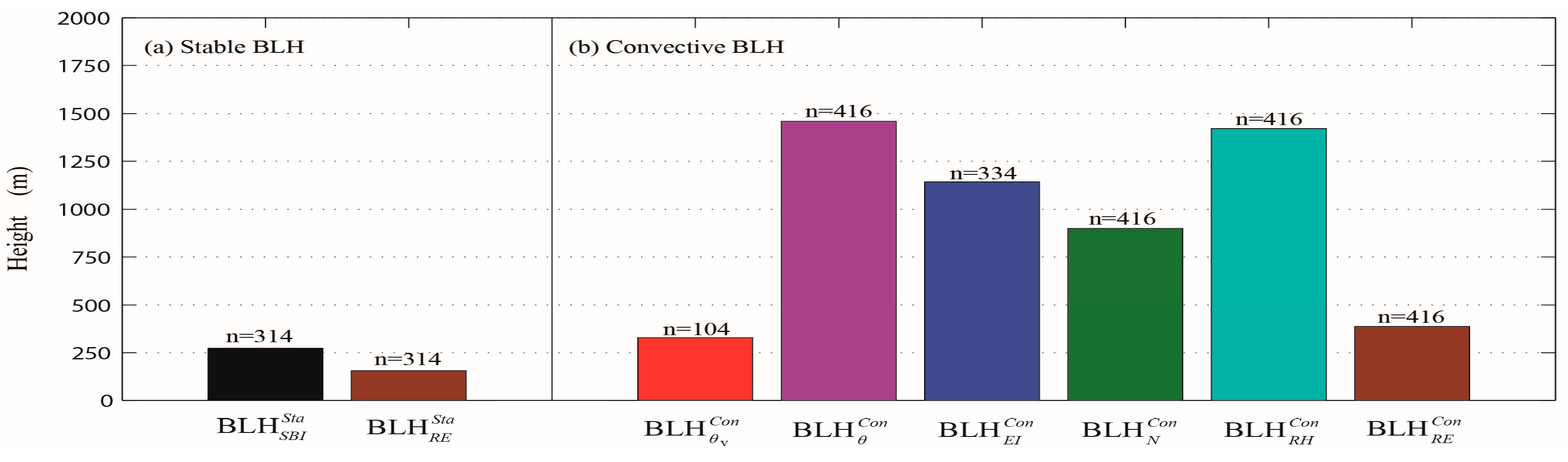
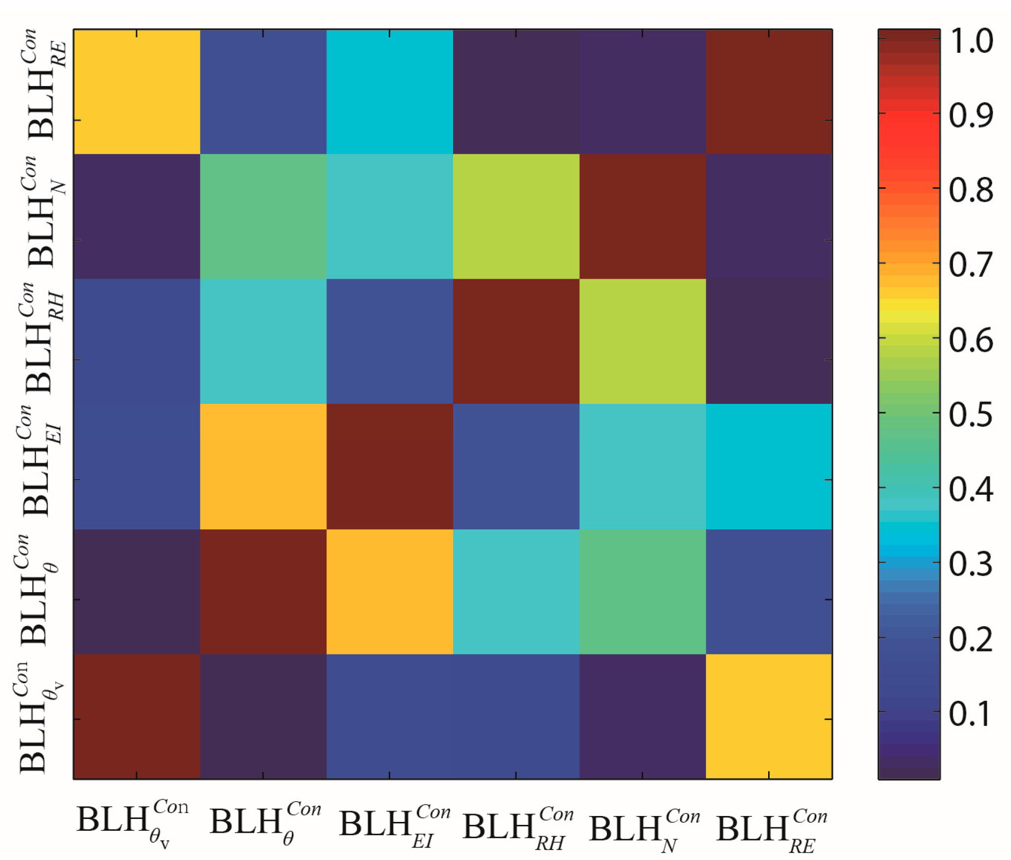
4.2. Statistical Comparison among Different BLH Methods

Figure 3 shows the averaged BLHs of Beijing during 2014–2015 calculated using the methods described in Section 3.1. The left two bars belong to the stable type of BLH, and the right bars belong to the convective type of BLH. The sample sizes are presented above the bars. The total sample size of sound profiles is 730 during 2014–2015. They are divided into two types based on the existence of a surface-based inversion layer. The sample size of stable BLH is 314, and that of the other is 416. Note that the sample size of ${\mathrm{BLH}}_{{\mathsf{\theta }}_{\mathrm{v}}}^{\mathrm{Con}}$ is only 104, which is much less than the sample size of the other convective BLHs. Most samples with the ${\mathrm{BLH}}_{{\mathsf{\theta }}_{\mathrm{v}}}^{\mathrm{Con}}$ are in summer and spring, since the sunrise is early in the morning for these two seasons. The surface temperature and ${\mathsf{\theta }}_{\mathrm{v}}$ quickly increase after sunrise, and the boundary layer will transform from stable to convective. However, the boundary layer is more likely to be neutral in the seasons of autumn and winter, and there is not a ${\mathsf{\theta }}_{\mathrm{v}}$ on the aloft profile equal to the surface ${\mathsf{\theta }}_{\mathrm{v}}$ for these samples with neutral stratification. We can increase the sample sizes of ${\mathrm{BLH}}_{{\mathsf{\theta }}_{\mathrm{v}}}^{\mathrm{Con}}$ by adding an excess ${\mathsf{\delta }\mathsf{\theta }}_{\mathrm{v}}$ on the surface ${\mathsf{\theta }}_{\mathrm{v}}$ [17]. However, it is difficult to determine the ${\mathsf{\delta }\mathsf{\theta }}_v$ using the radiosonde data for its coarse vertical levels. In addition, the sample size of ${\mathrm{BLH}}_{\mathrm{EI}}^{\mathrm{Con}}$ is also less than the sample sizes of other convective BLHs, because there are a few samples without elevated inversion in the total samples of the convective boundary layer [18].

In Figure 3, the stable type of BLH (two bars on the left) is significantly lower than the convective type of BLH (six bars on the right). This is because the stable boundary layer with negative buoyancy flux suppresses turbulence and results in a lower BLH, whereas the convective boundary layer with positive buoyancy flux enhances turbulence and results in a higher BLH [15,18]. Although the BLHs of the convective type are higher than the BLHs of the stable type, the BLHs within the same type also show significant differences. For the stable type of BLH, the ${\mathrm{BLH}}_{\mathrm{RE}}^{\mathrm{Sta}}$ is lower than the ${\mathrm{BLH}}_{\mathrm{SBI}}^{\mathrm{Sta}}$ by about 117 m. Moreover, there is a negative correlation coefficient (R = −0.29) between these two BLHs (Figure 4).

Because the ${\mathrm{BLH}}_{\mathrm{SBI}}^{\mathrm{Sta}}$ is estimated from the sounding profile data, it should more closely approximate to the actual situation of BLH. Thus, it is concluded that the ${\mathrm{BLH}}_{\mathrm{RE}}^{\mathrm{Sta}}$derived from the reanalysis products may be inaccurate, due to the horizontal and temporal resolution of the model, as well as the difference in BLH definition in the model [49,50,51]. It should be noted that the method of estimating BLH in the model is not based on the temperature inversion, which is different than the method of estimating ${\mathrm{BLH}}_{\mathrm{SBI}}^{\mathrm{Sta}}$. Thus, the correlation between ${\mathrm{BLH}}_{\mathrm{SBI}}^{\mathrm{Sta}}$ and ${\mathrm{BLH}}_{\mathrm{RE}}^{\mathrm{Sta}}$ is low.

For the convective type of BLH, the correlations between the six BLHs vary greatly, but most of them are low (Figure 5). Except for the squares along the diagonal line, which indicate auto-correlation of 1.0, the highest correlation is between ${\mathrm{BLH}}_{\mathsf{\theta }}^{\mathrm{Con}}$ and ${\mathrm{BLH}}_{\mathrm{EI}}^{\mathrm{Con}}$ at about 0.66. A possible explanation for this is that these two BLHs are estimated using the temperature profile. The second highest correlation is between ${\mathrm{BLH}}_{{\mathsf{\theta }}_{\mathrm{v}}}^{\mathrm{Con}}$ and ${\mathrm{BLH}}_{\mathrm{RE}}^{\mathrm{Con}}$ at 0.63, and the correlation between ${\mathrm{BLH}}_{\mathrm{RE}}^{\mathrm{Con}}$ and ${\mathrm{BLH}}_{\mathrm{EI}}^{\mathrm{Con}}$ also reaches 0.35. It seems that the ${\mathrm{BLH}}_{\mathrm{RE}}^{\mathrm{Con}}$ is relatively reliable for the convective boundary layer compared to ${\mathrm{BLH}}_{\mathrm{RE}}^{\mathrm{Sta}}$ for the stable boundary layer. A possible reason for this is that the variation within the convective BLH is large, and the tendency of BLH from the model usually agrees with that from the sounding profiles. In Figure 5, the lowest correlation is between ${\mathrm{BLH}}_{{\mathsf{\theta }}_{\mathrm{v}}}^{\mathrm{Con}}$ and ${\mathrm{BLH}}_{\mathrm{N}}^{\mathrm{Con}}$ at just about 0.01, which indicates that these two BLHs are approximately independent. In addition, the correlations between${\mathrm{BLH}}_{\mathrm{RH}}^{\mathrm{Con}}$ and ${\mathrm{BLH}}_{\mathrm{RE}}^{\mathrm{Con}}$, ${\mathrm{BLH}}_{\mathrm{N}}^{\mathrm{Con}}$ and ${\mathrm{BLH}}_{\mathrm{RE}}^{\mathrm{Con}}$, ${\mathrm{BLH}}_{{\mathsf{\theta }}_{\mathrm{v}}}^{\mathrm{Con}}$ and ${\mathrm{BLH}}_{\mathsf{\theta }}^{\mathrm{Con}}$ are also less than 0.1. Thus, these BLHs will result in different effects on the regression model of AOD-PM_2.5.

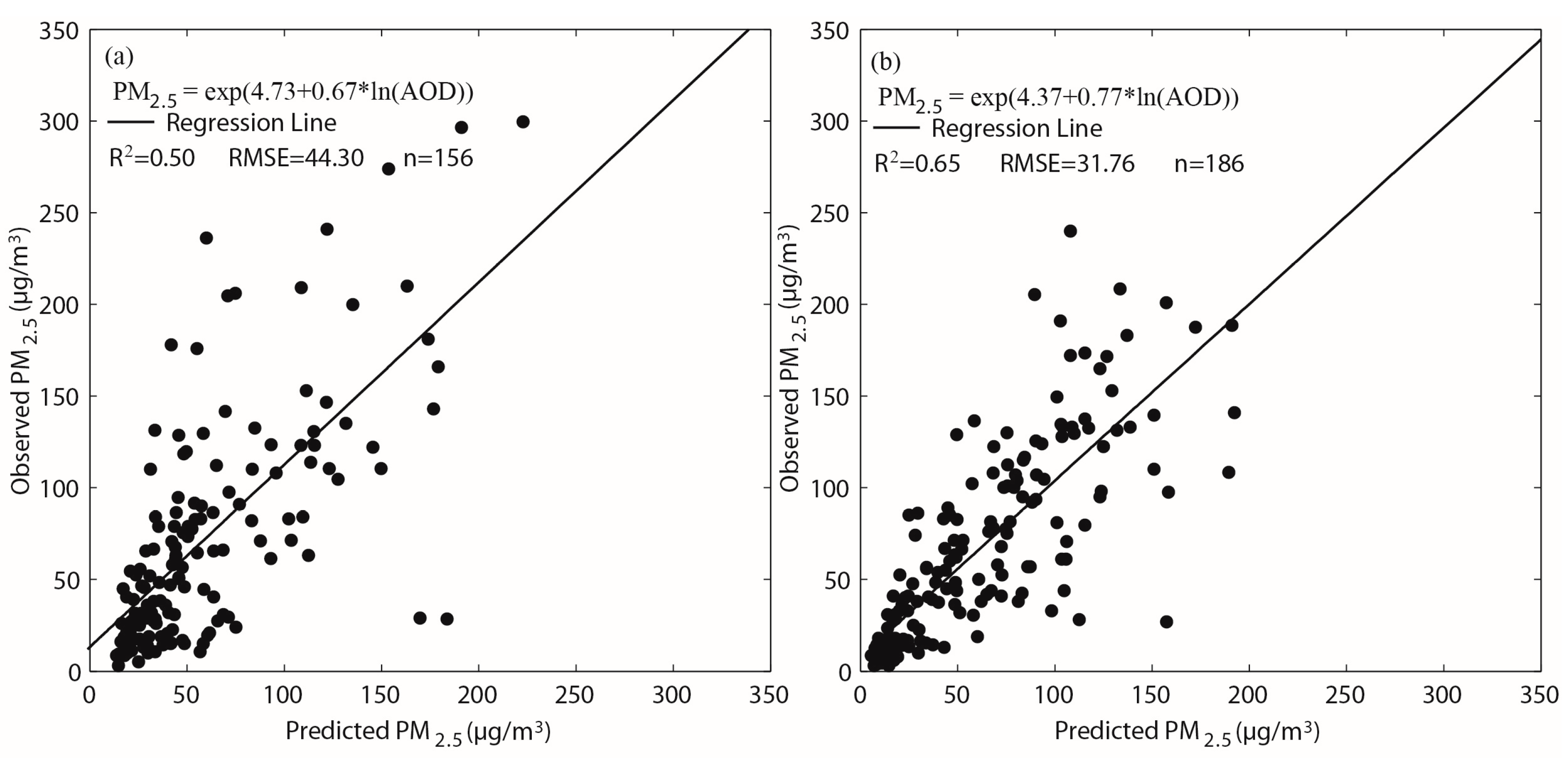
4.3. Performances of Simple Lognormal Models

A simple lognormal model (M-I) was developed to describe the relationship between surface PM_2.5 concentrations and AOD. To analyze the performance of the model for the two types of boundary layers, the M-I was divided into two types for the stable boundary layer (M-I-Sta) and the convective boundary layer (M-I-Con). There are 342 samples after matching the AOD and PM_2.5 data during 2014–2015. These samples are also divided into two parts for the two types of models. There are 156 and 186 samples for the M-I-Sta and M-I-Con after matching, respectively.

Figure 6a shows the scatter plot of observed vs. predicted surface PM_2.5 concentrations derived from the M-I-Sta. This model can explain 50% (R² = 0.50) of the variability in the corresponding PM_2.5 concentrations. The RMSE of this regression model is 44.30 µg/m³. For the M-I-Con (Figure 6b), the R² is 0.65 and the RMSE is 31.76 µg/m³, which is superior to the results of the M-I-Sta. It is found that there are some points with a large observed concentration but small predicted concentration that decrease the accuracy of the M-I-Sta (Figure 6a). We reasoned that while the observed PM_2.5 may be large, it may exhibit a low AOD in the M-I-Sta, because the surface-based inversion can inhibit the turbulent diffusion of aerosols by acting like a lid [52]. However, aerosols are relatively uniformly mixed in the convective boundary layer. Thus, the prediction accuracy of the M-I-Con is higher than that of the M-I-Sta.

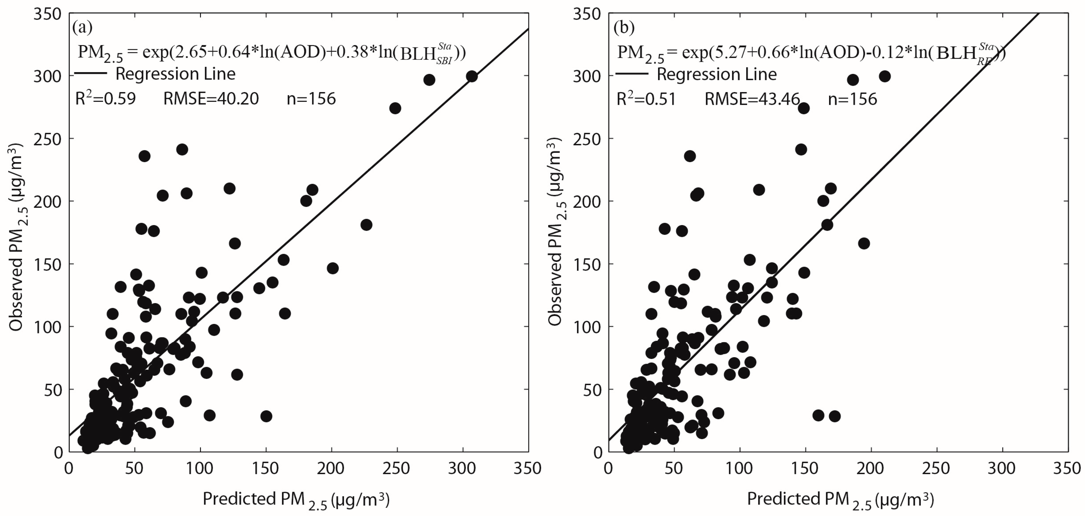
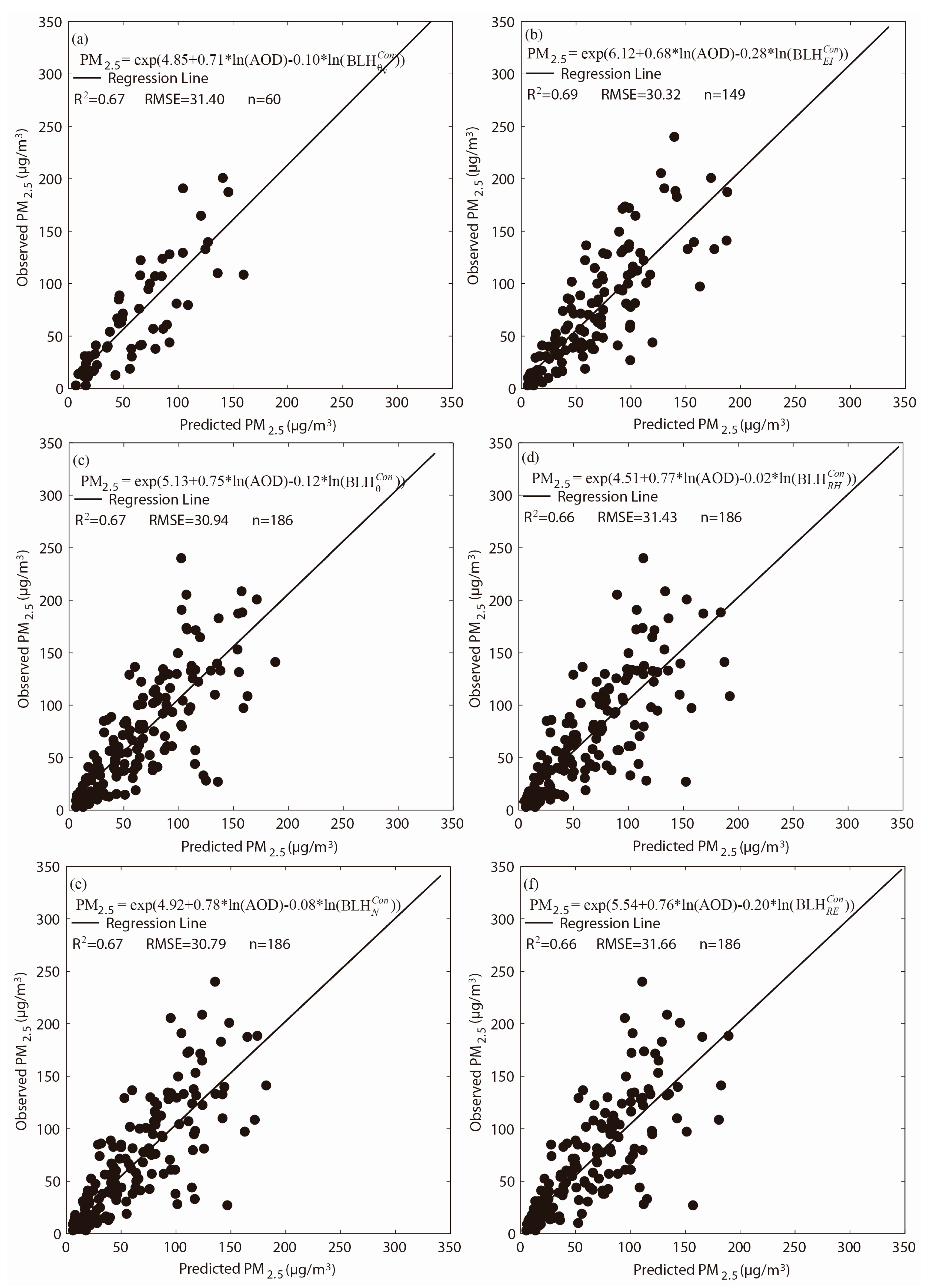
4.4. Ability of Different Blhs to Estimate Surface PM_2.5 Concentrations

In this section, the BLH values from different methods were added into the M-I to develop a new model, M-II, according to Equation (5). The M-II was also developed for the stable BLH (M-II-Sta) and convective BLH (M-II-Con), respectively. We expect to find the optimal BLHs out of the two stable BLHs and six convective BLHs. The samples of the M-II-Sta and the M-II-Con should be matched with the BLH based on the samples of the M-I-Sta and the M-I-Con, respectively. There are 156 samples for the M-II-Sta. For the M-II-Con, however, the sample sizes vary with the different convective BLHs. There are 60 and 149 samples after matching with ${\mathrm{BLH}}_{{\mathsf{\theta }}_{\mathrm{v}}}^{\mathrm{Con}}$ and ${\mathrm{BLH}}_{\mathrm{EI}}^{\mathrm{Con}}$, respectively. There are 186 samples after matching with ${\mathrm{BLH}}_{\mathsf{\theta }}^{\mathrm{Con}}$, ${\mathrm{BLH}}_{\mathrm{RH}}^{\mathrm{Con}}$, ${\mathrm{BLH}}_{\mathrm{N}}^{\mathrm{Con}}$ and ${\mathrm{BLH}}_{\mathrm{RE}}^{\mathrm{Con}}$.

Figure 7 shows the scatter plots of the observed versus the predicted surface PM_2.5 concentrations for the results of the M-II-Sta. The R² of the M-II-Sta with ${\mathrm{BLH}}_{\mathrm{SBI}}^{\mathrm{Sta}}$ (R² = 0.59, Figure 7a) is significantly higher than the R² of the M-I-Sta (R² = 0.50, Figure 5a), but the R² of the M-II-Sta with ${\mathrm{BLH}}_{\mathrm{RE}}^{\mathrm{Sta}}$ (R² = 0.51, Figure 7b) is similar to the R² of the M-I-Sta. The results indicate that ${\mathrm{BLH}}_{\mathrm{SBI}}^{\mathrm{Sta}}$ but not ${\mathrm{BLH}}_{\mathrm{RE}}^{\mathrm{Sta}}$ can effectively improve the model performance for the prediction of PM_2.5. Moreover, the regression coefficient associated with ${\mathrm{BLH}}_{\mathrm{SBI}}^{\mathrm{Sta}}$ is 0.38 (Figure 7a), but the regression coefficient associated with ${\mathrm{BLH}}_{\mathrm{RE}}^{\mathrm{Sta}}$ is −0.12 (Figure 7b). This is consistent with the negative correlation between ${\mathrm{BLH}}_{\mathrm{SBI}}^{\mathrm{Sta}}$ and ${\mathrm{BLH}}_{\mathrm{RE}}^{\mathrm{Sta}}$ shown in Figure 3. We suggest that the positive regression coefficient is reasonable, since a higher ${\mathrm{BLH}}_{\mathrm{SBI}}^{\mathrm{Sta}}$ means a deeper inversion that strongly inhibits the diffusion of surface pollution and increases the PM_2.5 concentration [53,54,55,56,57].

Figure 8 shows the results of the M-II-Con with the ${\mathrm{BLH}}_{{\mathsf{\theta }}_{\mathrm{v}}}^{\mathrm{Con}}$, ${\mathrm{BLH}}_{\mathrm{EI}}^{\mathrm{Con}}$, ${\mathrm{BLH}}_{\mathsf{\theta }}^{\mathrm{Con}}$, ${\mathrm{BLH}}_{\mathrm{RH}}^{\mathrm{Con}}$, ${\mathrm{BLH}}_{\mathrm{N}}^{\mathrm{Con}}$, and ${\mathrm{BLH}}_{\mathrm{RE}}^{\mathrm{Con}}$, respectively. The performance of the M-II-Con with ${\mathrm{BLH}}_{\mathrm{EI}}^{\mathrm{Con}}$ is optimal, with R² = 0.69 (Figure 8b), and the performance of the M-II-Con with ${\mathrm{BLH}}_{\mathrm{RE}}^{\mathrm{Con}}$ is the worst, with R² = 0.66 and RMSE = 31.66 µg/m³ (Figure 8f). It was found that the performance differences were not significant among these models of BLHs. Note that the regression coefficients associated with convective BLHs are all negative, and the largest is −0.28 (Figure 8b). It can be inferred that a higher convective BLH means a higher bottom of inversion. As such, the negative regression coefficient for convective BLH indicates that PM_2.5 concentrations from the surface are diluted in the boundary layer as convective BLH increases. However, the regression coefficient associated with the ${\mathrm{BLH}}_{\mathrm{SBI}}^{\mathrm{Sta}}$ is positive in Figure 6a, since there is not a lifting of the bottom of the surface-based inversion but rather a stronger inhibition of aerosol diffusion. Thus, the effects of the BLH on the model of AOD-PM_2.5 are contrary for the stable and convective boundary layers.

4.5. Optimal Model to Estimate Surface PM_2.5 Concentrations

The ${\mathrm{BLH}}_{\mathrm{SBI}}^{\mathrm{Sta}}$ shows optimal performance in the M-II-Sta, and the ${\mathrm{BLH}}_{\mathrm{EI}}^{\mathrm{Con}}$ shows optimal performance in the M-II-Con model. Thus, these two BLHs are still used as factors in the stepwise regression model of the M-III-Sta and the M-III-Con, respectively. The sample size of the M-III-Sta is 156, the same as the sample size of the M-II-Sta. For the M-III-Con, the samples size for the M-III-Con is 149, the same as the sample size of ${\mathrm{BLH}}_{\mathrm{EI}}^{\mathrm{Con}}$ in M-II-Con.

Table 3. Results of the stepwise regression of M-III-Sta (sample size n = 156).

M-III-Sta	Independent Variable	R2	RMSE
1	AOD (0.67 **)	0.50	44.30
2	AOD (0.52 **),RHsur (0.02 **)	0.62	38.73
3	AOD (0.53 **), RHsur (0.01 **),${\mathrm{BLH}}_{\mathrm{SBI}}^{\mathrm{Sta}}$ (0.28 **)	0.65	37.02
4	AOD (0.53 **), RHsur (0.01 **),${\mathrm{BLH}}_{\mathrm{SBI}}^{\mathrm{Sta}}$ (0.23 **),Tsur(−0.01 *)	0.68	35.44

Note: the numbers in parentheses represent the regression coefficients of stepwise regression model; * and ** at the upper right corner of number represent statistically significant at the 0.05 and 0.01 level, respectively.

shows the results of the stepwise regression of the M-III-Sta. The optimal regression is the fourth equation, which includes the factors of surface relative humidity (RH_sur), ${\mathrm{BLH}}_{\mathrm{SBI}}^{\mathrm{Sta}}$, and surface temperature (T_sur). The AOD, RH_sur, and ${\mathrm{BLH}}_{\mathrm{SBI}}^{\mathrm{Sta}}$ are all significant at the 99% confidence level (α = 0.01), and T_sur is significant at the 95% confidence level (α = 0.05). By introducing these factors, the R² increases from 0.50 to 0.68, and the RMSE decreases from 44.30 to 35.44 µg/m³. The first-order factor’s influence on the two-variate regression (AOD-PM_2.5) is RH_sur, which improves the R² from 0.50 to 0.62, and the second-order factor is ${\mathrm{BLH}}_{\mathrm{SBI}}^{\mathrm{Sta}}$, which improves the R² from 0.62 to 0.65. Note that there is a more significant improvement if the factor of ${\mathrm{BLH}}_{\mathrm{SBI}}^{\mathrm{Sta}}$ is introduced first (Figure 6a), such that the R² increases from 0.50 to 0.59. This is because of the complex correlation between ${\mathrm{BLH}}_{\mathrm{SBI}}^{\mathrm{Sta}}$, RH_sur, and PM_2.5. The influence of ${\mathrm{BLH}}_{\mathrm{SBI}}^{\mathrm{Sta}}$ on PM_2.5 is partly represented by RH_sur in the second or third equation of Table 3, which decreases the improvement of the ${\mathrm{BLH}}_{\mathrm{SBI}}^{\mathrm{Sta}}$. It could be inferred that a higher ${\mathrm{BLH}}_{\mathrm{SBI}}^{\mathrm{Sta}}$ means a stronger surface-based inversion layer that inhibits the diffusion of water vapor and aerosols, subsequently raising the RH_sur and PM_2.5. Thus, the regression coefficients of ${\mathrm{BLH}}_{\mathrm{SBI}}^{\mathrm{Sta}}$ and RH_sur are all positive in the equation for predicting PM_2.5. In the fourth equation of Table 3, the regression coefficient of T_sur is negative (−0.01). It may be speculated that a higher T_sur means a weaker surface-based inversion that decreases the surface PM_2.5. In a word, the influences of these factors on the PM_2.5 are all reasonable based on the correlation between surface-based inversion and PM_2.5.

Table 4. Results of the stepwise regression of the M-III-Con (sample size n = 149).

M-III-Con	Independent Variable	R2	RMSE
1	AOD (0.77 **)	0.65	31.76
2	AOD (0.68 **),${\mathrm{BLH}}_{\mathrm{EI}}^{\mathrm{Con}}$(−0.28 **)	0.69	30.32
3	AOD (0.67 **),${\mathrm{BLH}}_{\mathrm{EI}}^{\mathrm{Con}}$(−0.19 **),WSsur (−0.22 **)	0.70	29.89

Note: the numbers in parentheses represent the regression coefficients of stepwise regression model; ** at the upper right corner of number represent statistically significant at the 0.05 and 0.01 level, respectively.

shows the results of the stepwise regression of the M-III-Con. The optimal regression is the third equation, which includes the factors of AOD, ${\mathrm{BLH}}_{\mathrm{EI}}^{\mathrm{Con}}$, and surface wind speed (WS_sur). By introducing these factors, the R² increases from 0.65 to 0.70 and the RMSE decreases from 31.76 to 29.89 µg/m³. The first-order factor’s influence on the two-variate regression (AOD-PM_2.5) is ${\mathrm{BLH}}_{\mathrm{EI}}^{\mathrm{Con}}$, which improves the R² from 0.65 to 0.69. The second-order factor is WS_sur, which slightly improves the R² from 0.69 to 0.70; no other significant factors are introduced into the stepwise regression. It is suggested that the prediction accuracy is difficult to improve for the model of the convective type since the aerosol is uniformly mixed in this situation. Moreover, in the situation of the convective boundary layer, RH_sur is also uniformly mixed and its value is usually less than 80% near the ground. There are only 14 samples with the RH_sur being greater than 80% out of all 186 samples. The influence of humidity on the correlation of AOD-PM_2.5 is small because of the slight aerosol hygroscopic growth in the condition of RH_sur less than 80% [58,59]. Unlike RH_sur, the factor of WS_sur may vary greatly in the convective boundary layer. A higher WS_sur means a stronger convective process and a higher ${\mathrm{BLH}}_{\mathrm{EI}}^{\mathrm{Con}}$, but a lower PM_2.5. As such, the regression coefficient of WS_sur is negative (−0.22) in the optimal stepwise equation of Table 4. However, the WS_sur is not introduced in the stepwise equation of Table 3, since it is generally small in the stable boundary layer [60,61,62]. Thus, the number, order and effect of factors in the stepwise equation depend on the boundary layer types.

5. Conclusions

To evaluate the effect of the BLH on the regression model of AOD-PM_2.5, we divided the BLH into the stable and convective boundary types. These two types of boundary layer obviously exhibit seasonal difference. The percentage of the stable boundary layer is highest for winter. In contrast, the percentage of the stable boundary layer is lowest for summer. In addition, these two types of BLH are estimated by several different calculation methods, respectively. The stable BLH is estimated by the method of the top of surface-based inversion layer from the radiosonde profile (${\mathrm{BLH}}_{\mathrm{SBI}}^{\mathrm{Sta}}$) and by the method of interpolation from NCEP reanalysis (${\mathrm{BLH}}_{\mathrm{RE}}^{\mathrm{Sta}}$). The convective BLH is estimated by the methods using the profiles of virtual potential temperature (${\mathrm{BLH}}_{{\mathsf{\theta }}_{\mathrm{v}}}^{\mathrm{Con}}$), potential temperature (${\mathrm{BLH}}_{\mathsf{\theta }}^{\mathrm{Con}}$), elevated temperature inversion (${\mathrm{BLH}}_{\mathrm{EI}}^{\mathrm{Con}}$), relative humidity (${\mathrm{BLH}}_{\mathrm{RH}}^{\mathrm{Con}}$), refractivity (${\mathrm{BLH}}_{\mathrm{N}}^{\mathrm{Con}}$), and by another method from NCEP reanalysis (${\mathrm{BLH}}_{\mathrm{RE}}^{\mathrm{Con}}$). It is found that there are significant differences among the BLHs determined by these methods. The correlation between the two stable BLH of ${\mathrm{BLH}}_{\mathrm{SBI}}^{\mathrm{Sta}}$ and ${\mathrm{BLH}}_{\mathrm{RE}}^{\mathrm{Sta}}$ is even negative (−0.29). Moreover, the correlations between the convective BLHs are all lower than 0.70 with the lowest being 0.01. The differences between these BLHs could cause different regression coefficients and prediction accuracies in the regression model of AOD-PM_2.5.

The regression model of AOD-PM_2.5 is also divided into stable and convective types according the type of the BLH. For the model with AOD as the only factor, it is found that the prediction accuracy of the model for the stable type (M-I-Sta) is significantly lower than that of the model for the convective type (M-I-Con). After the BLH was introduced into the regression models (M-II-Sta and M-II-Con), the improvement of BLH for the M-II-Sta is more significant than that for the M-II-Con. For the M-II-Sta, the optimal BLH is ${\mathrm{BLH}}_{\mathrm{SBI}}^{\mathrm{Sta}}$, which improved the R² from 0.50 to 0.59. For the M-II-Con, the optimal BLH is ${\mathrm{BLH}}_{\mathrm{EI}}^{\mathrm{Con}}$, which improved the R² from 0.65 to 0.69. It is found that the regression coefficient of ${\mathrm{BLH}}_{\mathrm{SBI}}^{\mathrm{Sta}}$ in the M-II-Sta is positive, but the regression coefficient of ${\mathrm{BLH}}_{\mathrm{EI}}^{\mathrm{Con}}$ in the M-II-Con is negative. This result suggests that that the effects of BLH are contrary in the types of stable and convective boundary layers.

Based on the M-II-Sta and the M-II-Con models with the optimal BLH, other surface meteorological parameters were introduced into the regression model (M-III-Sta and M- III-Con) using the stepwise regression method. For the M-III-Sta, the optimal regression improved the R² from 0.50 to 0.68, which included the factors of surface relative humidity, ${\mathrm{BLH}}_{\mathrm{SBI}}^{\mathrm{Sta}}$, and surface temperature. The surface relative humidity is the first-order factor with a positive coefficient. For the M-III-Con, the optimal regression included the factors of ${\mathrm{BLH}}_{\mathrm{EI}}^{\mathrm{Con}}$ and surface wind speed. It is found that the number and the order of factors are different in the two types of models, and the effects of the meteorological factors on the model also closely related to the types of BLHs.

Most notably, this is the first study to our knowledge to investigate the effectiveness of BLH on the regression model of PM_2.5-AOD with respect to the stable and convective boundary layers. Our results provide compelling evidence for varying effects and mechanism of these two types of BLHs. However, our results are encouraging and should be validated for more radiosonde stations. In addition, methods to improve the accuracy of the PM_2.5-AOD model for areas without radiosonde data and only with reanalysis data should also be studied in future work.

References

1. Pope, C.A.; Burnett, R.T.; Thun, M.J.; Calle, E.E.; Krewski, D.; Ito, K.; Thurston, G.D. Lung cancer, cardiopulmonary mortality, and long-term exposure to fine particulate air pollution. JAMA 2002, 287, 1132–1141. [Google Scholar] [CrossRef] [PubMed]
2. Kappos, A.D.; Bruckmann, P.; Eikmann, T.; Englert, N.; Heinrich, U.; Hoppe, P.; Koch, E.; Krause, G.H.; Kreyling, W.G.; Rauchfuss, K.; et al. Health effects of particles in ambient air. Int. J. Hyg. Environ. Health 2004, 207, 399–407. [Google Scholar] [CrossRef] [PubMed]
3. Miller, K.A.; Siscovick, D.S.; Sheppard, L.; Sullivan, J.H.; Anderson, G.L.; Kaufman, J.D. Long-term exposure to air pollution and incidence of cardiovascular events in women. N. Engl. J. Med. 2007, 356, 447–458. [Google Scholar] [CrossRef] [PubMed]
4. Sacks, J.D.; Stanek, L.W.; Luben, T.J.; Johns, D.O.; Buckley, B.J.; Brown, J.S.; Ross, M. Review particulate matter–induced health effects: Who is susceptible? Environ. Health Perspect. 2011, 119, 446–454. [Google Scholar] [CrossRef] [PubMed]
5. Wang, J.; Christopher, S.A. Intercomparison between satellite-derived aerosol optical thickness and PM2.5 mass: Implications for air quality studies. Geophys. Res. Lett. 2003, 30, 267–283. [Google Scholar] [CrossRef]
6. Van Donkelaar, A.; Martin, R.V.; Park, R.J. Estimating ground-level PM2.5 using aerosol optical depth determined from satellite remote sensing. J. Geophys. Res. Atoms. 2006, 111, 5049–5066. [Google Scholar]
7. Hoff, R.M.; Christopher, S.A. Remote sensing of particulate pollution from space: Have we reached the promised land? J. Air Waste Manag. Assoc. 2009, 59, 642–644. [Google Scholar]
8. Tian, J.; Chen, D. A semi-empirical model for predicting hourly ground-level fine particulate matter (PM2.5) concentration in southern Ontario from satellite remote sensing and ground-based meteorological measurements. Remote Sens. Environ. 2010, 14, 221–229. [Google Scholar] [CrossRef]
9. Li, C.; Hsu, N.C.; Tsay, S.C. A study on the potential applications of satellite data in air quality monitoring and forecasting. Atmos. Environ. 2011, 45, 3663–3675. [Google Scholar] [CrossRef]
10. Tao, J.H.; Zhang, M.G.; Chen, L.F.; Wang, Z.F.; Su, L.; Ge, C.; Han, X.; Zou, M.M. A method to estimate concentrations of surface-level particulate matter using satellite-based aerosol optical thickness. Sci. China Earth Sci. 2013, 56, 1422–1433. [Google Scholar] [CrossRef]
11. Koelemeijer, R.; Homan, C.; Matthijsen, J. Comparison of spatial and temporal variations of aerosol optical thickness and particulate matter over Europe. Atmos. Environ. 2006, 40, 5304–5315. [Google Scholar] [CrossRef]
12. You, W.; Zang, Z.L.; Pan, X.B.; Zhang, L.F.; Chen, D. Estimating PM2.5 in Xi'an, China using aerosol optical depth: A comparison between the MODIS and MISR retrieval models. Sci. Total Environ. 2015, 505, 1156–1165. [Google Scholar] [CrossRef] [PubMed]
13. Liu, Y.; Franklin, M.; Kahn, R.; Koutrakis, P. Using aerosol optical thickness to predict ground-level PM2.5, concentrations in the St. Louis area: A comparison between MISR and MODIS. Remote Sens. Environ. 2007, 107, 33–44. [Google Scholar] [CrossRef]
14. Gupta, P.; Christopher, S.A. Particulate matter air quality assessment using integrated surface, satellite, and meteorological products: Multiple regression approach. J. Geophys. Res. 2009, 114. [Google Scholar] [CrossRef]
15. Stull, R.B. An Introduction to Boundary Layer Meteorology; Kluwer Academic Publishers: Dordrecht, The Netherlands, 1998; p. 666. [Google Scholar]
16. Garratt, J.R. The Atmospheric Boundary Layer; Cambridge University Press: Cambridge, UK, 1992; p. 335. [Google Scholar]
17. Seibert, P.; Beyrich, F.; Gryning, S.E.; Joffre, S.; Rasmussen, A.; Tercier, P. Review and intercomparison of operational methods for the determination of the mixing height. Atmos. Environ. 2000, 34, 1001–1027. [Google Scholar] [CrossRef]
18. Seidel, D.J.; Ao, C.O.; Li, K. Estimating climatological planetary boundary layer heights from radiosonde observations: Comparison of methods and uncertainty analysis. J. Geophys. Res. 2010, 115, D16113. [Google Scholar] [CrossRef]
19. Bradley, R.S.; Keimig, F.T.; Diaz, H.F. Recent changes in the North American Arctic boundary layer in winter. J. Geophys. Res. 1993, 98, 8851–8858. [Google Scholar] [CrossRef]
20. Wang, X.Y.; Wang, K.C. Homogenized variability of radiosonde-derived atmospheric boundary layer height over the global land surface from 1973 to 2014. J. Clim. 2016, 29, 6893–6908. [Google Scholar] [CrossRef]
21. Basha, G.; Ratnam, M.V. Identification of atmospheric boundary layer height over a tropical station using high resolution radiosonde refractivity profiles: Comparison with GPS radio occultation measurements. J. Geophys. Res. 2009, 114, D16101. [Google Scholar] [CrossRef]
22. Ferrero, L.; Riccio, A.; Perrone, M.; Sangiorgi, G.; Ferrini, B.S.; Bolzacchini, E. Mixing height determination by tethered balloon-based particle soundings and modeling simulations. Atmos. Res. 2011, 102, 145–156. [Google Scholar] [CrossRef]
23. Durre, I.; Vose, R.S.; Wuertz, D.B. Overview of the integrated global radiosonde archive. J. Clim. 2006, 19, 53–68. [Google Scholar] [CrossRef]
24. Durre, I.; Yin, X. Enhanced radiosonde data for studies of vertical structure. Bull. Am. Meteorol. Soc. 2008, 89, 1257–1262. [Google Scholar] [CrossRef]
25. Li, W. Technical Assessment Report of L-Band Upper Air Sounding System; China Meteorological Press: Beijing, China, 2009; p. 95. [Google Scholar]
26. Seidel, D J; Zhang, Y.; Beljaars, A.; Golaz, J.; Jacobson, A.R.; Medeiros, B. Climatology of the planetary boundary layer over the continental United States and Europe. J. Geophys. Res. Atoms. 2012, 117, 127–135. [Google Scholar] [CrossRef]
27. Holben, B.N.; Eck, T.F.; Slutsker, I.; Tanré, D.; Buis, J.P.; Setzer, A.; Vermote, E.; Reagan, J.A.; Kaufman, Y.J.; Nakajima, T.; et al. AERONET—A federated instrument network and data archive for aerosol characterization. Remote Sens. Environ. 1998, 66, 1–16. [Google Scholar] [CrossRef]
28. Holben, B.N.; Tanré, D.; Smirnov, A.; Eck, T.F.; Slutsker, I.; Abuhassan, N.; Newcomb, W.W.; Schafer, J.S.; Chatenet, B.; Lavenu, F.; et al. An emerging ground-based aerosol climatology: Aerosol optical depth from AERONET. J. Geophys. Res. 2001, 106, 12067–12097. [Google Scholar] [CrossRef]
29. Tripathi, S.N.; Dey, S.; Chandel, A.; Srivastava, S.; Singh, R.P.; Holben, B.N. Comparison of MODIS and AERONET derived aerosol optical depth over the Ganga Basin, India. Ann. Geophys. 2005, 23, 1093–1101. [Google Scholar] [CrossRef]
30. Ge, J.M.; Su, J.; Fu, Q.; Ackerman, T.P.; Huang, J.P. Dust aerosol forward scattering effects on ground-based aerosol optical depth retrievals. J. Quant. Spectrosc. Radiat. Transf. 2011, 112, 310–319. [Google Scholar] [CrossRef]
31. Xia, X.A.; Chen, H.B.; Wang, P.C. Validation of MODIS aerosol retrievals and evaluation of potential cloud contamination in East Asia. J. Environ. Sci. 2004, 16, 832–837. [Google Scholar]
32. Li, X. Validation of Aerosol Optical Thickness Product over China with MODIS Data Operated at NSMC. J. Appl. Meteorol. Sci. 2009, 20, 147–156. [Google Scholar]
33. Qi, Y.L.; Ge, J.M.; Huang, J.P. Spatial and temporal distribution of MODIS and MISR aerosol optical depth over northern China and comparison with AERONET. Chin. Sci. Bull. 2013, 58, 2497–2506. [Google Scholar] [CrossRef]
34. Munchak, L.A.; Levy, R.C.; Mattoo, S.; Remer, L.A. MODIS 3 km aerosol product: Applications over land in an urban/suburban region. Atmos. Meas. Tech. 2013, 6, 1747–1759. [Google Scholar] [CrossRef]
35. Schaap, M.; Apituley, A.; Timmermans, R.M.A.; Koelemeijer, R.B.A.; Leeuw, G.D. Exploring the relation between aerosol optical depth and PM2.5 at Cabauw, the Netherlands. Atmos. Chem. Phys. 2008, 9, 909–925. [Google Scholar] [CrossRef]
36. Tao, R; Che, H.Z.; Chen, Q.L.; Tao, J; Wang, Y.Q.; Sun, J.Y.; Wang, H.; Zhang, X.Y. Study of aerosol optical properties based on ground measurements over Sichuan Basin, China. Aerosol. Air. Qual. Res. 2014, 14, 905–915. [Google Scholar] [CrossRef]
37. You, W.; Zang, Z.L.; Zhang, L.F.; Li, Z.J.; Chen, D.; Zhang, G. Estimating ground-level PM10 concentration in northwestern China using geographically weighted regression based on satellite AOD combined with CALIPSO and MODIS fire count. Remote Sens. Environ. 2015, 168, 276–285. [Google Scholar] [CrossRef]
38. Hong, S.Y. Nonlocal boundary layer vertical diffusion in a medium-range forecast model. Mon. Weather. Rev. 1996, 124, 2322. [Google Scholar] [CrossRef]
39. Han, J; Witek, M.L.; Teixeira, J.; Sun, R.Y.; Pan, H.L.; Fletcher, J.K.; Bretherton, C.S. Implementation in the NCEP GFS of a Hybrid Eddy-Diffusivity Mass-Flux (EDMF) Boundary Layer Parameterization with Dissipative Heating and Modified Stable Boundary Layer Mixing. Weather Forecast. 2016, 31, 341–352. [Google Scholar] [CrossRef]
40. National Centers for Environmental Prediction Climate Forecast System. Available online: http://cfs.ncep.noaa.gov/ (accessed on 29 January 2013).
41. Holzworth, G.C. Estimates of mean maximum mixing depths in the contiguous United States. Mon. Weather Rev. 1964, 92, 235–242. [Google Scholar] [CrossRef]
42. Oke, T.R. Boundary Layer Climates, 2nd ed.; Halsted Press: New York, NY, USA, 1988; p. 435. [Google Scholar]
43. Sorbjan, Z. Structure of the Atmospheric Boundary Layer; Prentice Hall: Englewood Cliffs, NJ, USA, 1989; p. 317. [Google Scholar]
44. Ao, C.O.; Waliser, D.E.; Chan, S.K.; Li, J.L.; Tian, B.J.; Xie, F.Q.; Mannucci, A.J. Planetary boundary layer heights from GPS radio occultation refractivity and humidity profiles. J. Geophys. Res. Atoms. 2012, 117, D16117. [Google Scholar] [CrossRef]
45. Sokolovskiy, S.; Kuo, Y.H.; Rocken, C.; Schreiner, W.S.; Hunt, D.; Anthes, R.A. Monitoring the atmospheric boundary layer by GPS radio occultation signals recorded in the open-loop mode. Geophys. Res. Lett. 2006, 33, L12813. [Google Scholar] [CrossRef]
46. Xie, F.; Wu, D.L.; Ao, C.O.; Mannucci, A.J.; Kursinski, E.R. Advances and limitations of atmospheric boundary layer observations with GPS occultation over southeast Pacific Ocean. Atmos. Chem. Phys. 2012, 12, 903–918. [Google Scholar] [CrossRef]
47. Wang, X.Y.; Wang, K.C. Estimation of atmospheric mixing layer height from radiosonde data. Atmos. Meas. Tech. 2014, 7, 1701–1709. [Google Scholar] [CrossRef]
48. Song, W.Z.; Jia, H.F.; Huang, J.F.; Zhang, Y.Y. A satellite-based geographically weighted regression model for regional PM2.5 estimation over the Pearl River Delta region in China. Remote Sens. Environ. 2014, 154, 1–7. [Google Scholar] [CrossRef]
49. Lazar, A.; Vintzileos, A.; Doblas-Reyes, F.J.; Rogel, P.; Delecluse, P. Seasonal forecast of tropical climate with coupled ocean–atmosphere general circulation models: On the respective role of the atmosphere and the ocean components in the drift of the surface temperature error. Tellus A 2005, 57, 387–397. [Google Scholar] [CrossRef]
50. Zhao, T.; Guo, W.; Fu, C. Calibrating and evaluating reanalysis surface temperature error by topographic correction. J. Clim. 2008, 21, 1440–1446. [Google Scholar] [CrossRef]
51. Wang, S.; Zhang, M.; Sun, M.; Wang, B.; Huang, X.Y.; Wang, Q.; Feng, F. Comparison of surface air temperature derived from NCEP/DOE R2, ERA-interim, and observations in the arid northwestern China: A consideration of altitude errors. Theor. Appl. Climatol. 2015, 119, 99–111. [Google Scholar] [CrossRef]
52. Li, J.; Chen, H.B.; Li, Z.Q.; Wang, P.C.; Cribb, M.; Fan, X.H. Low-level temperature inversions and their effect on aerosol condensation nuclei concentrations under different large-scale synoptic circulations. Adv. Atmos. Sci. 2015, 32, 898–908. [Google Scholar] [CrossRef]
53. Malek, E.; Davis, T.; Martin, R.S.; Silva, P.J. Meteorological and environmental aspects of one of the worst national air pollution episodes (January, 2004) in Logan, Cache Valley, Utah, USA. Atmos. Res. 2006, 79, 108–122. [Google Scholar] [CrossRef]
54. Silva, P.J.; Vawdrey, E.L.; Corbett, M.; Erupe, M. Fine particle concentrations and composition during wintertime inversions in Logan, Utah, USA. Atmos. Environ. 2007, 41, 5410–5422. [Google Scholar] [CrossRef]
55. Sun, Y.; Wang, Y.S.; Zhang, C.C. Vertical observations and analysis of PM2.5, O3, and NOx at Beijing and Tianjin from tower during summer and autumn 2006. Adv. Atmos. Sci. 2010, 27, 123–136. [Google Scholar] [CrossRef]
56. Chu, D.A.; Tsai, T.C.; Chen, J.P.; Chang, S.C.; Jeng, Y.J.; Chang, W.L.; Lin, M.H. Interpreting aerosol lidar profiles to better estimate surface PM 2.5, for columnar AOD measurements. Atmos. Environ. 2013, 79, 172–187. [Google Scholar] [CrossRef]
57. Liu, S.; Min, H.S.S.; He, L.Y.; Niu, Y.W.; Bruegemann, B.; Gnauk, T.; Herrmann, H. Size distribution and source analysis of ionic compositions of aerosols in polluted periods at Xinken in Pearl River Delta (PRD) of China. Atmos. Environ. 2008, 42, 6284–6295. [Google Scholar] [CrossRef]
58. Zhang, Y.; Li, Z. Estimation of PM2.5 from fine-mode aerosol optical depth. J. Remote Sens. 2013, 17, 929–943. [Google Scholar]
59. Lin, C.; Li, Y.; Yuan, Z.; Lau, A.K.H.; Li, C.C.; Fung, J.C.H. Using Satellite Remote Sensing Data to Estimate the High-Resolution Distribution of Ground-Level PM2.5. Remote Sens. Environ. 2015, 156, 117–128. [Google Scholar] [CrossRef]
60. Chenge, Y.; Brutsaert, W. Flux-profile relationships for wind speed and temperature in the stable atmospheric boundary layer. Bound. Layer Meteorol. 2005, 114, 519–538. [Google Scholar] [CrossRef]
61. Kelley, N.D.; Jonkman, B.J. The Stable Atmospheric Boundary Layer: A Challenge for Wind Turbine Operations. Proceedings of AGU Fall Meeting, San Francisco, CA, USA, 15–19 December 2008. [Google Scholar]
62. Mahrt, L. Characteristics of submeso winds in the stable boundary layer. Bound. Layer Meteorol. 2009, 130, 1–14. [Google Scholar] [CrossRef]
Figure 1. The spatial distribution of the PM2.5 station, radiosonde station and Aerosol Robotic Network (AERONET) station used in this study.
Atmosphere 08 00104 g001
Figure 2. The average vertical temperature profiles of stable BLH and convective BLH for spring (a), summer (b), autumn (c) and winter (d).
Atmosphere 08 00104 g002
Figure 3. Average BLHs of stable boundary layer (a) and convective boundary layer (b) in Beijing during 2014–2015 calculated by different methods.
Atmosphere 08 00104 g003
Figure 4. Scatter plot of BLH SBI Sta vs. BLH RE Sta .
Atmosphere 08 00104 g004
Figure 5. Cross-correlations between convective BLHs from six different methods.
Atmosphere 08 00104 g005
Figure 6. Scatter plots of the observed vs. the predicted surface PM2.5 concentrations for the M-I-Sta (a) and the M-I-Con (b).
Atmosphere 08 00104 g006
Figure 7. Scatter plots of the observed vs. the predicted surface PM2.5 concentrations from the M-II-Sta with BLH SBI Sta (a) and BLH RE Sta (b).
Atmosphere 08 00104 g007
Figure 8. Scatter plots of the observed vs. the predicted surface PM2.5 concentrations from the M-II-Con with BLH θ v Con (a), BLH EI Con (b), BLH θ Con (c), BLH RH Con (d), BLH N Con (e) and BLH RE Con (f).
Atmosphere 08 00104 g008