Street-Level Ventilation in Hypothetical Urban Areas


Department of Mechanical Engineering, The University of Hong Kong, Hong Kong, China
*
Author to whom correspondence should be addressed.
†
These authors contributed equally to this work.
Atmosphere 2017, 8(7), 124; https://doi.org/10.3390/atmos8070124
Submission received: 11 May 2017
/
Revised: 5 July 2017
/
Accepted: 10 July 2017
/
Published: 16 July 2017
(This article belongs to the Special Issue Recent Advances in Urban Ventilation Assessment and Flow Modelling)
Abstract
:Street-level ventilation is often weakened by the surrounding high-rise buildings. A thorough understanding of the flows and turbulence over urban areas assists in improving urban air quality as well as effectuating environmental management. In this paper, reduced-scale physical modeling in a wind tunnel is employed to examine the dynamics in hypothetical urban areas in the form of identical surface-mounted ribs in crossflows (two-dimensional scenarios) to enrich our fundamental understanding of the street-level ventilation mechanism. We critically compare the flow behaviors over rough surfaces with different aerodynamic resistance. It is found that the friction velocity is appropriate for scaling the dynamics in the near-wall region but not the outer layer. The different freestream wind speeds () over rough surfaces suggest that the drag coefficient (= ) is able to characterize the turbulent transport processes over hypothetical urban areas. Linear regression shows that street-level ventilation, which is dominated by the turbulent component of the air change rate (ACH), is proportional to the square root of drag coefficient . This conceptual framework is then extended to formulate a new indicator, the vertical fluctuating velocity scale in the roughness sublayer (RSL) , for breathability assessment over urban areas with diversified building height. Quadrant analyses and frequency spectra demonstrate that the turbulence is more inhomogeneous and the scales of vertical turbulence intensity are larger over rougher surfaces, resulting in more efficient street-level ventilation.
1. Introduction
Cities are growing [1], with over of the global population currently residing in these areas [2]. Megacities might allow for more efficient energy consumption at the expense of diversified air-pollutant sources [3]. Knowledge accumulated to rectify these problems is therefore crucial to society. Concurrently, atmospheric flows, which cover a variety of length and time scales [4], are key factors governing the transport processes over urban areas with dynamics that strongly affect street-level air quality and pollutant removal. Engineering flows over rough surfaces are commonly used as the analytical platforms to enrich our fundamental understanding of urban atmospheric boundary layer (ABL) problems [5,6]. Typical applications include wind engineering for the built environment [7,8], particulate matter (PM) in street canyons [9], city breathability [10,11], and pedestrian wind comfort/safety [12] as well as guideline formulation [13]. Unlike their smooth-surface counterparts, the aerodynamic resistance induced by rough surfaces on turbulent boundary layers (TBLs) is less sensitive to the Reynolds number (= ; where U is the characteristic velocity scale of flows, h the characteristic length scale of roughness elements and the kinematic viscosity). Instead, it is largely influenced by the roughness geometries of surfaces that are commonly measured by blockage ratio (where is the TBL thickness), friction velocity (= ; where is the surface shear stress and the fluid density), zero-plane displacement and roughness length [14,15]. They are therefore critical (roughness) similarity parameters which should be monitored carefully in urban ABL modeling [16,17]. However, the same roughness parameters for different rough surfaces do not necessarily imply the same flow properties [18,19]. Besides, their effect on street-level ventilation is less studied. This study is therefore conceived, using reduced-scale physical modeling, to examine how surface roughness quantitatively affects the dynamics and the subsequent influence on street-level ventilation, facilitating innovation of urban planning guidelines from the pollutant removal [20] as well as urban heat island [21] perspective.
Apart from field measurements and mathematical modeling, wind tunnel experiments are common laboratory solutions to the transport processes over various land features [22,23,24]. Unlike their open-terrain counterparts, urban surfaces absorb momentum from the mean flows, converting it to turbulence kinetic energy (TKE) [25]. Surface roughness enhances wake flows and turbulence intensities [26], we therefore hypothesize that aerodynamic resistance, which is measured by drag coefficient (= ; where is the prevailing wind speed) in this paper, could serve as an indicator of street-level ventilation in urban areas. In the urban climate community, street-level ventilation is commonly assessed by the transfer coefficient , where is the passive-scalar transfer velocity [27,28]. The elevated transfer coefficient over urban areas is explained by the length-scale adjustment over rough surfaces [29]. The (time scale of) mass exchange between street canyons and the overlying urban-ABL flows is also measured by the cavity wash-out time [30]. Flushing, which refers to the the instantaneous, large-scale turbulence structures prevailing across the street canyons, plays a key role in aged air removal [31]. It is believed that the unsteady fluid exchanges between street canyons and the overlaying flows are mainly driven by the shear over the buildings [32]. Analogous to smooth-wall flows, ejection (Q2) [33] and sweep (Q4) [34] contribute most to the turbulent transport processes in near-surface region, reflecting the stronger momentum exchange over rough surfaces.
At high Reynolds number, the logarithmic law of the wall (log-law) is a fundamental part of mean-flow description [35] that applies to the inertial sublayer (ISL) over both smooth and rough surfaces [36]. Turbulence structures, such as fluctuating velocities and cross-correlations, are of the same type [37] over rough and smooth surfaces. While roughness effects are confined to the inner layer [38], recent studies revealed the roughness sublayer (RSL) in-between the ISL and roughness elements [39]. RSL scaling, because of the local dependence on individual roughness elements, is different from that in the ISL [40,41]. This feature, which is different from that over smooth surfaces, is attributed to the organized eddy structures in the near-surface region over rough surfaces [42]. An RSL velocity profile therefore departs from the conventional log-law relationship, eventually affecting the transport processes. An example is the surface fluxes of atmospheric constituents over urban areas [43]. In view of the diversified indicators for street-level ventilation and the recent findings in the RSL over urban canopy, a series of wind tunnel experiments are performed in attempt to refine the current indicator for street-level ventilation especially for flows over inhomogeneous buildings.
In this paper, we focus on the (rough) surface layer of the urban ABL in neighborhood scales [44] in attempt to examine how building morphology (e.g., regimes of skimming flow and isolated roughness) modifies the dynamics together with the implication to street-level ventilation. The functionality of drag coefficient , which is commonly used to measure aerodynamic resistance, is explored to estimate street-level ventilation. In addition to flow statistics, this paper looks into the intermittency in an attempt to demystify the correlation between building roughness and street-level ventilation performance. This section introduces the background, reviews the literatures and defines the problem statement. The methodology and solution approach are detailed in Section 2. The results, including flow properties and turbulence profiles, are interpreted in Section 3 before we propose a new ventilation indicator and look into the ventilation mechanism. Finally, the conclusions are drawn in Section 4.
2. Methodology
Wind tunnel experiments are conducted to address the research problem in this paper. An infinitely large, idealized urban surface is simulated by gluing an array of identical rib-type roughness elements (two-dimensional, 2D, scenarios). In contrast to the majority of wind tunnel studies in building science, in which arrays of three-dimensional (3D) roughness elements in the form of cuboids are mostly used, 2D roughness elements are adopted in the current study for comparison with our previous large-eddy simulation (LES). Moreover, the aerodynamic resistance over ribs is larger than that over cuboids that widens the range of drag coefficient being tested in the ventilation estimate. Our hypothetical urban models, though simplified, enable the fundamental understanding of rough-surface dynamics, fostering the theoretical framework for street-level ventilation.
2.1. Wind Tunnel Infrastructure
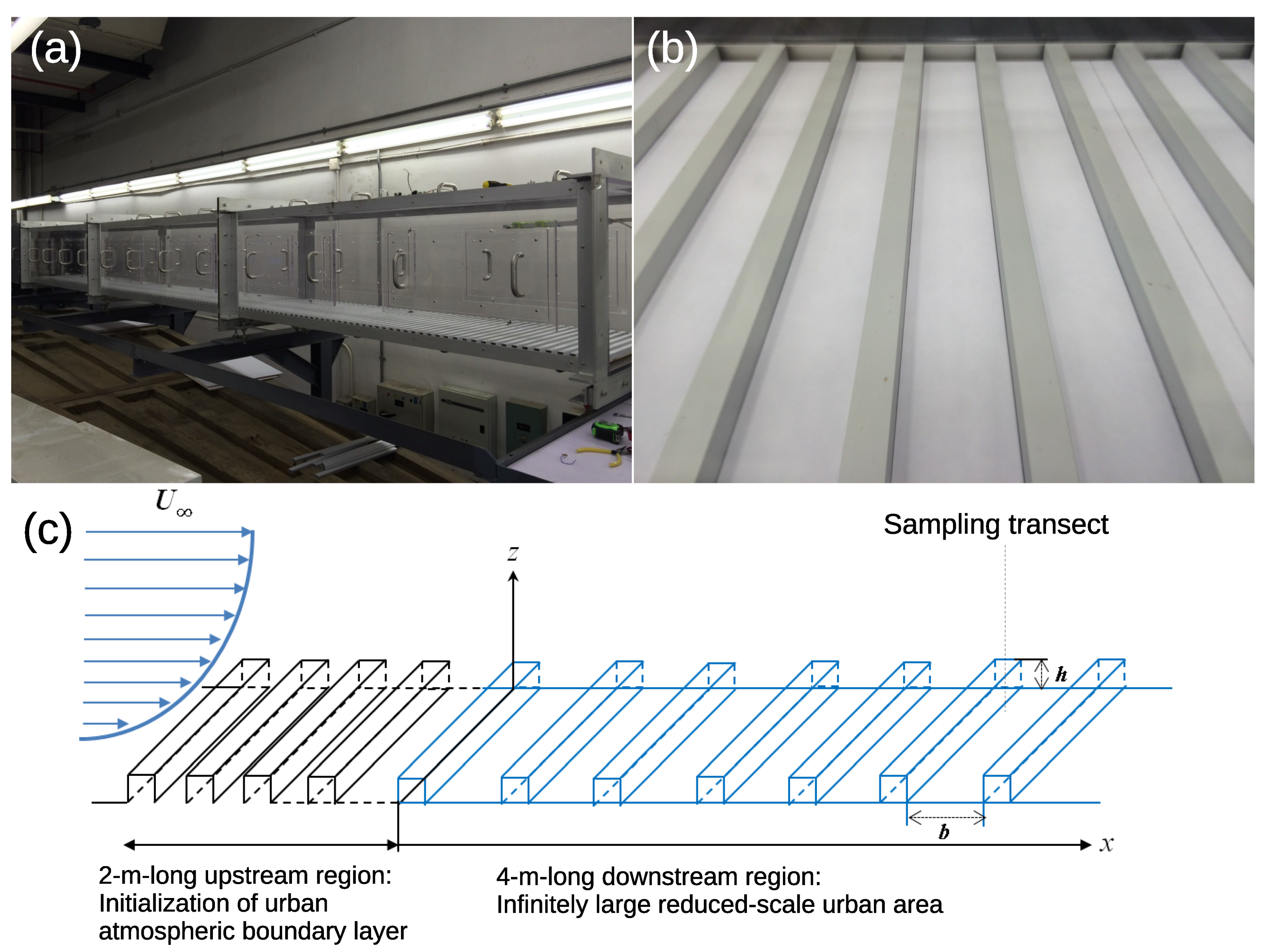
The experiments are carried out in the open-circuit, isothermal wind tunnel in the Department of Mechanical Engineering, University of Hong Kong (Figure 1). Its test section is made of acrylic whose size is 6000 mm (length) × 560 mm (width) × 560 mm (height). The flows are driven by a three-phase, electricity-powered blower and the wind speed is controlled (by a damper) in the range of m s ≤ ≤ 20 m s. A honeycomb is installed before the test section to straighten the flows as well as to reduce the turbulence intensity. Square aluminum tubes of size h (= 19 mm) are placed in crossflows at h apart in the first 2000 mm to initiate the TBL. The remaining 4000 mm downstream is reserved for the reduced-scale urban models.
2.2. Idealized Urban Surfaces
Hypothetical urban areas are fabricated by aligning square aluminum tubes of size h (= 19 mm) in crossflows. Eight types of rough surfaces in the form of ribs are adopted (Table 1). The wind-tunnel test floor is fully covered by baseboards (each 500 mm long × 560 mm wide × 5 mm thick) on which the aluminum tubes are glued. The streamwise extent of the array of aluminum ribs is 4000 mm that is sufficient for fully developed TBL flows. The aluminum tubes are 560 mm (≈ ) long, spanning the full width of the test section. They are placed at b (38 mm ≤ b ≤ 228 mm) apart to adjust the aspect ratio ( = ) in order to model the aerodynamic resistance of urban areas. The range of ARs covers the typical urban flow regimes (skimming flows, wake interference and isolated roughness) [45] that are analogous to the engineering rough-wall flow regimes (d-type and k-type) [46]. The test-section height is H (= 560 mm) so the roughness-element-height-to-test-section-height (blockage) ratio h:H is bounded by 1:28. This small blockage ratio ensures sufficient headroom in the wind-tunnel, enabling proper TBL development across the test section [47].
2.3. Hot-Wire Anemometry
The wind tunnel is equipped with a computer-controlled traversing system whose positioning accuracy is 1 mm. The system interface is the National Instruments (NI) motion control unit for probing flow samples. The flows are measured by hot-wire anemometry (HWA). A thin platinum-plated tungsten wire (-mm diameter), whose resistance is sensitivity to heat, is soldered to a sampling probe that is connected to a bridge circuit. It is cooled down by forced convection in flows, leading to a change in electrical resistance (measurable at high frequency). The bridge circuit then feeds back to adjust the voltage supply in order to maintain the hot wire at constant temperature. The HWA sampling frequency is up to Hz, facilitating the measurements of turbulence intensity and momentum flux.
In-house developed HWA and data acquisition systems are employed in this study. The hot wires are partly etched by copper-electroplating in which the effective sensing length is 2 mm. An X-wire design is used, which includes an angle between a pair of hot-wires of 100°. It measures two velocity components (streamwise u and vertical w) simultaneously and the large included angle (≥ 90°) reduces the potential error arising from the elevated turbulence level in the near-wall region. The hot-wire probe is connected to a constant-temperature anemometer which is basically the bridge circuit mentioned previously. The X-wire pair therefore consists of the parts of the resistance components in the circuit whose changes measure the flow velocities. A NI compactDAQ unit (NI cDAQ-9188), which has a processor for data conversion and temporary storage, is used to digitalize the analog signal. It is connected to a desktop computer via a Local Area Network (LAN) cable to avoid data loss. The data acquisition is then managed by the LabVIEW software to minimize the delay in real-time data transfer.
The universal conversion scheme for the 2-mm Institute of Sound and Vibration Research (ISVR) probe [48] is used to convert from voltage output to velocity reading. Each hot-wire probe has its own characteristic response so its thermal behavior is unique. A scaling coefficient is therefore required even it is operated at room temperature. Before measurement, the voltage output at calm-wind conditions is recorded which is then used to obtain a proper scaling for each hot-wire probe. All the hot-wire probes are also calibrated against uniform flows in the range of 1 m s ≤ ≤ m s prior for quality assurance.
The wind speed adopted in the current wind tunnel experiments is in the range of 8 m s ≤ ≤ m s. The Reynolds number based on freestream wind speed and TBL thickness (= ) is thus at least two orders of magnitude larger than the critical one (approximately 1200, irrespective of the state of the walls) [49] and hence the effect of molecular viscosity is negligible. The friction velocity measured is in the range of m s ≤ ≤ m s; the roughness Reynolds number (= ) is at least two orders of magnitude larger than unity [50] so the flows are fully developed. Therefore, our wind tunnel experiments are appropriate to model the TBL flows over rough surfaces. The parameters of the wind tunnel experiments are tabulated in Table 1.
3. Results and Discussion
We look into the wind-tunnel measured velocity profiles to examine the flows and TBL characteristics before analyzing the dynamics and ventilation estimate in detail. Between seven and nine vertical transects are used to sample the flow data over a unit of the street canyon. The vertical spatial resolution is in the range of 1 mm ≤ ≤ 10 mm stretching in the wall-normal direction. The first point is 5 mm over the roughness elements and the sampling height is up to 300 mm, covering the entire TBL. Afterward, we derive the new indicator measuring street-level ventilation. Finally, we look into the intermittency using quadrant analysis and frequency spectrum to elucidate ventilation mechanism.
3.1. Thickness of TBL and ISL
In this study, the TBL thickness is defined at the height where the spatio-temporal average of momentum flux is asymptotically approaching zero [51]. It in turn implies that the two velocity components u and w are no longer correlated. Here, angle brackets and the overbar represent spatial and temporal average of statistical flow properties, respectively. Double primes denote the deviation from the spatio-temporal average = . Under this circumstance, the dynamics are dominated by advection rather than the crosswind turbulent transport. This phenomenon can only be observed over the TBL where the intermittency resumes the prevailing flows. The TBL thickness observed in this paper is in the range of 200 mm ≤ ≤ 304 mm (Table 1).
The thickness of the inertial sublayer (ISL, where the logarithmic law of the wall applies) is determined by monitoring the momentum flux such that its variation in the wall-normal direction is less than a certain level. The vertical variation is measured by [52]:
Here is the mean of the spatio-temporal average of momentum flux that is calculated by five-point moving average in the wall-normal direction. In this study, the range of ISL is defined at z where ≤ ≤ after a series of sensitivity tests. The resolution of the current wind-tunnel measurements is too coarse to resolve the variation of down to . The roughness parameters, such as displacement height and roughness length , are determined subsequently.
3.2. Friction Velocity
Friction velocity is one of the key parameters in TBL flows over rough surfaces. It is the characteristic velocity to scale the near-surface turbulence in this paper. Among various methods, surface-level momentum flux is most commonly used to estimate the friction velocity [53]. For rough-surface flows, the turbulent momentum flux is much larger than its viscous counterpart [50] so it is reasonable to assume that as the estimate to friction velocity.
3.3. Wind Speed Profiles
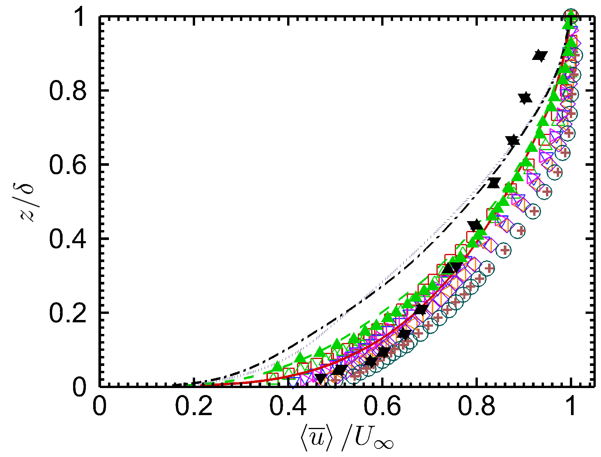
Figure 2 depicts the vertical profiles of spatio-temporally averaged wind speed over rib-type rough surfaces of different ARs. Although the range tested is narrow (from to ), the current wind-tunnel measured friction factor f generally increases with decreasing AR (widening the separation b between roughness elements; Table 1). The near-surface velocity gradient over different rough surfaces shows a similar behavior, i.e., velocity increases more sharply with increasing aerodynamic resistance, signifying the elevated drag in the near-surface region (Figure 2). The length scales of flows are highly correlated with the velocity gradient at different elevation [54]. The transport processes are therefore enhanced because of the more uniform wind speed over rougher surfaces, extending to the outer layer close to z = .
The current wind-tunnel measured wind-speed profiles are compared well to those calculated by LES [55] of ARs = and (Figure 2). For the other two cases with ARs = and , the LES-calculated near-surface velocity gradient is notably less than that of wind-tunnel data implying that the modeling turbulent transport processes are weaker than those measured in the wind tunnel experiments. Their surface velocity is so small that is slowed down by the sharp flow impingement on the windward wall of roughness elements. Apart from the smaller Reynolds number in the LES (by about two times), the difference could be attributed to the unavoidable turbulence production in the wind tunnel upstream, which, however, does not exist in the idealized horizontally homogeneous LES calculation. On top of roughness-generated turbulence, background turbulence enhances momentum transport so the the wind-tunnel mean wind speed is more uniform than its LES counterpart. The wind-speed profiles show a more favorable agreement in d-type flows than that in k-type. The LES spatial resolution could be an issue because a high spatial resolution is needed to resolve the flow impingement on the windward faces of roughness elements where recirculating flows dominate the dynamics.
Experimental results from other research groups are also adopted to verify the current wind-tunnel measurements (Figure 2). The experimental results agree reasonably well with each other in the near-surface region such that the data available in literature [56,57] fall within the range of current wind-tunnel measurements of k-type flows. A notable discrepancy is observed for z over (in the outer layer) that is attributed to the dissimilar modeling configuration in different wind-tunnel settings. The TBL thickness in [57] is around , more shallow than that of the current wind-tunnel measurements ( h h) by over , leading to a thinner near-surface region.
3.4. Turbulence Profiles
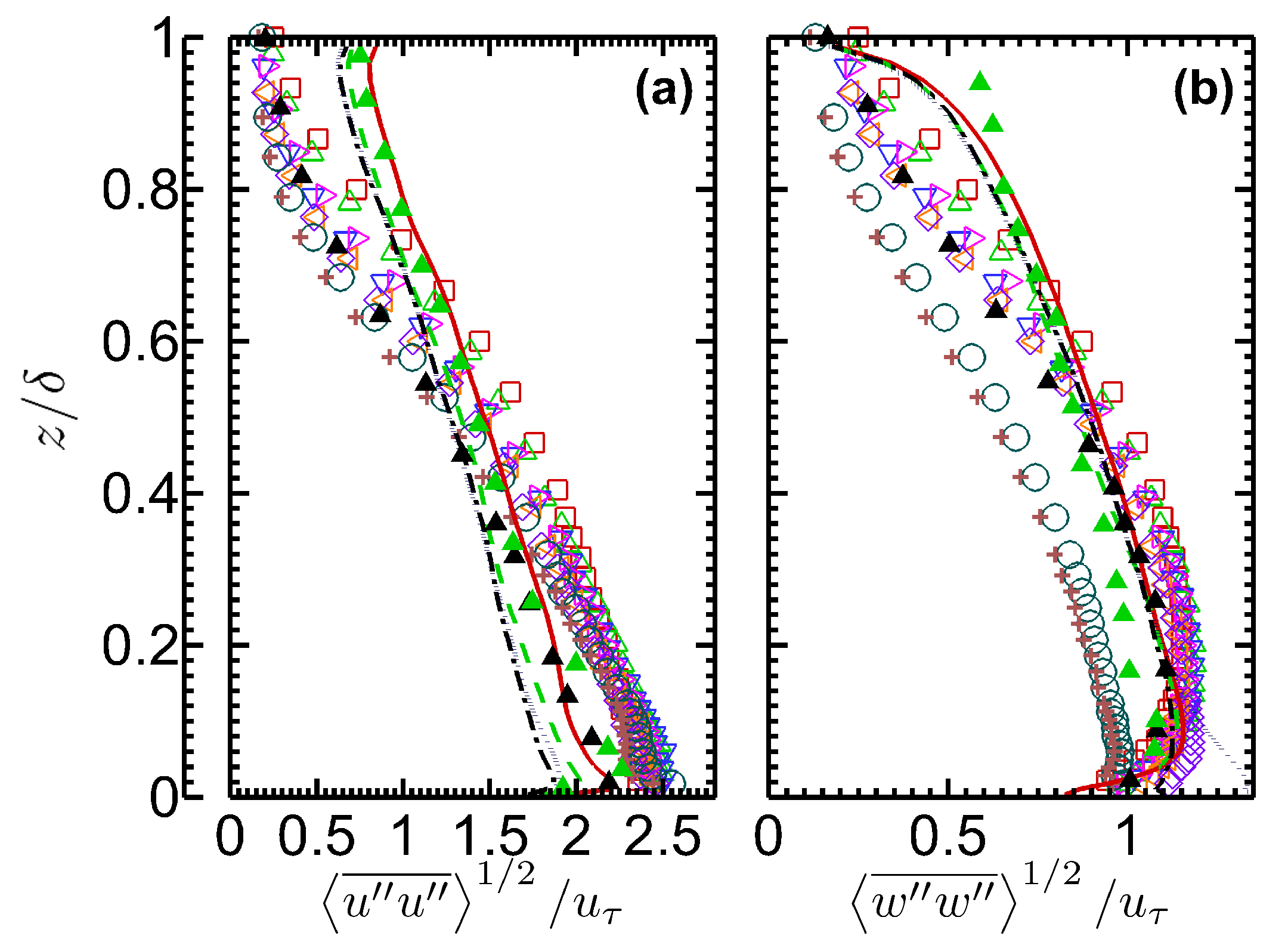
Vertical profiles of streamwise and vertical fluctuating velocities are illustrated in Figure 3a,b, respectively. Similar to most TBL studies of open-channel flows, the fluctuating velocities are scaled by the friction velocity . Rough-surface turbulence is more isotropic compared with its smooth-surface counterpart [58] so the difference between the two components, streamwise and vertical, is less. Streamwise fluctuating velocity decreases with increasing wall-normal distance (almost linearly). The profiles over different rough surfaces collapse well in the inner layer (), demonstrating the dominance of roughness-generated turbulence and the appropriateness of the velocity scale. Aloft the near-surface flows in , the dimensionless streamwise fluctuating velocity over different rough surfaces shows a mild dissimilarity that is caused by the background turbulence in the wind tunnel and the uncertainty of velocity scales. Rib-type surfaces are installed upstream to initialize TBL development in which the turbulence levels are relatively higher in the flows over smoother surfaces (larger ARs). Hence, the dimensionless streamwise fluctuating velocity decreases with increasing AR in ≤ z ≤ . Besides, the friction velocity , which decreases with smoother surfaces, is not the most appropriate characteristic scale to normalize the velocity in the outer region, leading to the discrepancy.
The current streamwise fluctuating velocity profiles compare more favorably with other wind-tunnel measurements available in literature [56,57] than do the LES. The different behavior observed is attributed to the dissimilar flow configurations in the physical and mathematical models. The LESs are calculated over idealized geometry in which the prevailing flows are driven by a uniform background pressure gradient. The friction velocity is calculated by the pressure gradient in the LES. The dynamics are therefore generally in line with those observed in theoretical open-channel flows. On the other hand, the flows in wind tunnels are driven by upstream speed that fall into the category of TBL flows. The flows are, though gradually, unavoidably developing over the urban models.
The current wind-tunnel measured profiles of vertical fluctuating velocity profiles show a behavior different from that of their streamwise counterparts. The surface-level vertical fluctuating velocities over different rough surfaces are comparable with each other ( ≤ ≤ ), supporting the scaling using friction velocity. Differences are generally grouped into two categories according to the nature of drag force. In the skimming flow or wake interference regimes (AR in the range of to ), the mean flows seldom descend from the TBL core down to the street canyon so the broad peak of vertical fluctuating velocity is elevated analogous to that over smooth surfaces [59]. On the other hand, because of the flow entrainment from the TBL core down to the street canyons, the drag mechanism in the flows in isolated roughness regime (AR in the range of 1:12 to 1:10), is dominated by flow impingement on the windward walls of roughness elements. The vertical fluctuating velocity is thus peaked at the surface level instead. It decreases thereafter with increasing wall-normal distance that ends up with a lower turbulence level compared with that in d-type flows. The smaller dimensionless vertical fluctuating velocity in the outer layer is also partly attributed to the larger friction velocity in k-type flows. The agreement in the vertical fluctuating velocity among the two experimental measurements and the LES results is good, though the k-type flows in wind tunnel show a lower dimensionless vertical fluctuating velocity.
Figure 4 compares the dimensionless profiles of spatio-temporally averaged momentum flux over different rough surfaces obtained in the current wind-tunnel measurements. Negative momentum flux signifies that the streamwise momentum is transported downward by the vertical fluctuating velocity. Hence, prevailing flows play key roles in near-surface turbulence generation and the associated transport processes. Apart from the mild surface-level reduction, the magnitude of momentum flux obtained from the two approaches consistently decreases with increasing wall-normal distance. Slight dissimilarity is observed. Because of the idealized configuration, the theoretical solution to the momentum flux in forced open-channel flows is a linear function of wall-normal distance. In the current wind tunnel experiments, on the other hand, a constant-flux region (in the inner layer) up to is clearly observed, assembling the general behavior in the atmospheric surface layer (ASL) where the logarithmic law of the wall applies [60]. Moreover, the decreasing rate of momentum flux slows down so the wind-tunnel measured profiles are not as linear as the theoretical ones in the outer layer . The over-predicted turbulence is due to the background turbulence level in the wind tunnels. It is noteworthy that 3D roughness elements produce turbulence scales of the order of the roughness height h while the motions generated by 2D roughness elements may be much larger due to the width of the roughness elements [61]. Rib-type roughness elements deviate from the similarity in the outer layer in the cases with 3D roughness and smooth walls [62]. While the authors are aware of the dissimilarity representing urban areas, the use of rib-type roughness elements in the current wind-tunnel experiments facilitates the comparison with the LES [55] in which a configuration of ribs in crossflows was adopted to reduce the computation load by ensemble averaging in the homogeneous spanwise direction.
3.5. Street-Level Ventilation Estimate
Roughness sublayer (RSL) dynamics over rough surfaces are crucial to surface-level turbulence generation. In the RSL, individual roughness elements have their own effects on the flows aloft, complicating the turbulence structure such that the conventional understanding of ISL no longer fully describes the dynamics and the ventilation mechanism. One of the examples is the TKE redistribution from vertical to spanwise components, resulting in decreasing anisotropy and turbulence scales [63,64]. While the RSL dynamics were examined in details in our previous study [65], such as the velocity profiles and length scale in RSL, this paper focuses on the practical significance of RSL particularly related to the street-level ventilation estimate.
For idealized urban street canyons, the air change rate [66],
was proposed, where is the width of a street canyon, in order to measure street-level ventilation by comparing the aged air removal (or the fresh air entrainment) [67]. It was found that the street-level ventilation is largely governed by its turbulent component (over ). Recently, analytical solutions and mathematical modeling consistently showed that exhibits a linear correlation with the square root of the drag coefficient [68]
It is hence proposed that the performance of street-level ventilation can be estimated once the drag coefficient of a specific urban area is available. However, originally proposed by [67] is calculated along the roof level of buildings of uniform height only. This definition of ventilation indicator is hardly implemented over urban areas practically such as building height variability. Moreover, street-level ventilation is governed by RSL dynamics but not those along building-roof level. Under this circumstance, a new indicator, which is able to handle urban areas with diversified building height and elevated RSL turbulence intensity, is proposed in this paper. The technical details are reported below.
In view of the importance of RSL dynamics, we switch the focus from building-roof level to the RSL. A new indicator, namely the RSL vertical velocity scale:
is therefore proposed as a ventilation indicator over urban areas. Here, is the RSL domain and the subscript + denotes the upward flows only. The effect of RSL turbulence on street-level ventilation is thus included. Figure 5 expresses the RSL vertical fluctuating velocity scale as a function of the square root of drag coefficient . Similar to the indicator defined in [67], a linear correlation is revealed in which the correlation coefficient is up to . This linear correlation suggests that the drag coefficient of urban areas could be used to parameterize the street-level ventilation performance.
3.6. Quadrant Analysis
In view of the important intermittency in the ventilation mechanism reflected by , Figure 6 compares the contributions from different quadrants to the turbulent momentum flux . Our definition of joint probability density function (JPDF) and the covariance integrand of the fluctuating velocities and are based on those suggested by [69],
The JPDF is calculated according to the ratio of the occurrences of individual quadrants to the total number of data samples. The quadrants are defined in Table 2. The JPDF measures the frequency of occurrence while the covariance integrand measures the strength of events. Figure 6 shows a wider range of turbulent intensity relative to the friction velocity for flows over street canyons of = 1:2 (d-type flows) compared with = 1:12 (k-type flows). Flows over both street canyons of = 1:2 and 1:12 exhibit more frequent events of sweep Q4 and ejection Q2, in line with the laboratory measurements over a single street canyon available in the literature [70]. For d-type flows over street canyons of = 1:2, illustrates a similar shape over building roofs and street canyons such that stronger sweeps Q4 and ejection Q2 are more frequent than outward interaction Q1 and inward interaction Q3. On the other hand, as shown by the JPDF, extreme events occur more frequently, which is likely attributed to the accelerating (decelerating) flow entrainment (removal), demonstrating their influence on street-level ventilation. The covariance integrand over the building roofs and street canyons are similar for flows over = 1:2, implying a more homogeneous transport process. In contrast, extreme events, as signified by the elevated covariance integrand (by five times) are observed for flows over street canyons of = 1:12, resulting in the more efficient street-level ventilation in wider streets. A wider street thus favors extreme events (stronger updraft and downdraft) for ventilation enhancement.
3.7. Frequency Spectrum
Fast Fourier transform (FFT) is used to convert the time traces of velocity from time to frequency domain. Figure 7 shows that the roof-level spectra over the arrays of hypothetical urban areas exhibit a conventional inertial subrange with a slope. The energy spectra cover almost five orders of magnitude of spatial/temporal scales. The low-frequency fraction () of streamwise turbulence scales is obviously stronger than its vertical counterpart by an order of magnitude. Contributions from high-frequency fractions are about the same, demonstrating the isotropic nature of small-scale turbulence. This finding also concurs the importance of extreme events in a street-level ventilation mechanism which is discussed in Section 3.6 previously. No notable difference in streamwise turbulence spectra over buildings and street canyons is observed. However, a mild difference is shown in the vertical turbulence spectra. The low-frequency fraction over building roofs is slightly higher than that over street canyons and is attributed to the higher level of velocity shear near the solid boundary, enhancing mechanical turbulence generation. Moreover, it is interesting that the low-frequency fraction of turbulence-intensity spectra over street canyons of = 1:12 is higher than that of 1:2. Hence, the turbulence scales governing street-level ventilation in wider street canyons are stronger.
4. Conclusions
In view of the importance of air quality, a series of wind tunnel experiments are sought to elucidate the mechanism of street-level ventilation in urban areas. Vertical profiles of mean wind speed illustrate that the near-surface velocity gradient is large, leading to the drag and enhanced transport processes. Examination of the profiles of fluctuating velocities and momentum flux suggests that friction velocity is an appropriate quantity to scale the inner-layer turbulence quantities but not those in the outer layer. In the spatio-temporally averaged turbulence statistics, the streamwise fluctuating velocity is peaked at the roof level while the vertical fluctuating velocity has relatively broad maxima. These observations are consistent with previous findings in literature [71]. A new indicator, the vertical fluctuating velocity scale in roughness sublayer , is proposed to measure the street-level ventilation performance over urban areas of different aerodynamic resistance and building height variability. Major benefits include its applicability to areas with inhomogeneous buildings and the (linear) correlation with (the square root of) drag coefficient that facilities sensitivity tests in design stage. Nevertheless, additional tests are required to unveil the limitations and drawbacks in a practical perspective. Because street-level ventilation is mainly driven by turbulence, quadrant analysis and frequency spectrums are carried out. Similar to the flows over smooth surfaces, vertical turbulent transport is dominated by sweep and ejection. The inertial subrange is exhibited in the wind tunnel measurements as well.
Acknowledgments
The first author wishes to thank the Hong Kong Research Grants Council (RGC) for financially supporting his study through the Hong Kong PhD Fellowship (HKPF) scheme. This project is partly supported by the General Research Fund (GRF) of RGC HKU 17210115.
Author Contributions
Yat-Kiu Ho and Chun-Ho Liu conceived and designed the experiments; Yat-Kiu Ho performed the experiments; Yat-Kiu Ho and Chun-Ho Liu analyzed the data and wrote the paper.
Conflicts of Interest
The authors declare no conflict of interest.
References
- Deweerdt, S. The urban downshift. Nature 2016, 531, S52–S53. [Google Scholar] [CrossRef] [PubMed]
- Wigginton, N.S.; Fahrenkamp-Uppenbrink, J.; Wible, B.; Malakoff, D. Cities are the future. Science 2016, 352, 904–905. [Google Scholar] [CrossRef] [PubMed]
- Parrish, D.D.; Zhu, T. Clean air for megacities. Science 2009, 326, 674–675. [Google Scholar] [CrossRef] [PubMed]
- Fernando, H.J.S. Fluid dynamics of urban atmospheres in complex terrain. Annu. Rev. Fluid Mech. 2010, 42, 365–389. [Google Scholar] [CrossRef]
- Claus, J.; Krogstad, P.A.; Castro, I.P. Some measurements of surface drag in urban-type boundary layers at various wind angles. Bound. Layer Meteorol. 2012, 145, 407–422. [Google Scholar] [CrossRef]
- Ricci, A.; Burlando, M.; Freda, A.; Repetto, M.P. Wind tunnel measurements of the urban boundary layer development over a historical district in Italy. Build. Environ. 2017, 111, 192–206. [Google Scholar] [CrossRef]
- Tse, K.T.; Hitchcock, P.A.; Kwok, K.C.S.; Thepmongkorn, S.; Chan, C.M. Economic perspectives of aerodynamic treatments of square tall buildings. J. Wind Eng. Ind. Aerodyn. 2009, 97, 455–467. [Google Scholar] [CrossRef]
- Aly, A.M. Atmospheric boundary-layer simulation for the built environment: Past, present and future. Build. Environ. 2014, 75, 206–221. [Google Scholar] [CrossRef]
- Stabile, L.; Arpino, F.; Buonanno, G.; Russi, A.; Frattolillo, A. A simplified benchmark of ultrafine particle dispersion in idealized urban street canyons: A wind tunnel study. Build. Environ. 2015, 93, 186–198. [Google Scholar] [CrossRef]
- Panagiotou, I.; Neophytou, M.K.A.; Hamlyn, D.; Britter, R.E. City breathability as quantified by the exchange velocity and its spatial variation in real inhomogeneous urban geometries: An example from central London urban area. Sci. Total Environ. 2013, 442, 466–477. [Google Scholar] [CrossRef] [PubMed]
- Hang, J.; Wang, Q.; Chen, X.; Sandberg, M.; Zhu, W.; Buccolieri, R.; Di Sabatino, S. City breathability in medium density urban-like geometries evaluated through the pollutant transport rate and the net escape velocity. Build. Environ. 2015, 94, 166–182. [Google Scholar] [CrossRef]
- Blocken, B.; Stathopoulos, T.; van Beeck, J.P.A.J. Pedestrian-level wind conditions around buildings: Review of wind-tunnel and CFD techniques and their accuracy for wind comfort assessment. Build. Environ. 2016, 100, 50–81. [Google Scholar] [CrossRef]
- Kubota, T.; Miura, M.; Tominaga, Y.; Mochida, A. Wind tunnel tests on the relationship between building density and pedestrian-level wind velocity: Development of guidelines for realizing acceptable wind environment in residential neighborhoods. Build. Environ. 2008, 43, 1699–1708. [Google Scholar] [CrossRef]
- Jiménez, J. Turbulent flows over rough walls. Annu. Rev. Fluid Mech. 2004, 36, 173–196. [Google Scholar] [CrossRef]
- Kamruzzaman, M.; Djenidi, L.; Antonia, R.A.; Talluru, K.M. Drag of a turbulent boundary layer with transverse 2D circular rods on the wall. Exp. Fluids 2015, 56, 121–129. [Google Scholar] [CrossRef]
- Hagishima, A.; Tanimoto, J.; Nagayama, K.; Meno, S. Aerodynamic parameters of regular arrays of rectangular blocks with various geometries. Bound. Layer Meteorol. 2009, 132, 315–337. [Google Scholar] [CrossRef]
- Karimpour, A.; Kaye, N.B.; Baratian-Ghorghi, Z. Modeling the neutrally stable atmospheric boundary layer for laboratory scale studies of the built environment. Build. Environ. 2012, 49, 203–211. [Google Scholar] [CrossRef]
- Krogstad, P.-Å.; Antonia, R.A. Surface roughness effects in turbulent boundary layers. Exp. Fluids 1999, 27, 450–460. [Google Scholar] [CrossRef]
- Antonia, R.A.; Krogstad, P.-Å. Turbulence structure in boundary layers over different types of surface roughness. Fluid Dyn. Res. 2001, 28, 139–157. [Google Scholar] [CrossRef]
- Mirzaei, P.A.; Haghighat, F. Pollution removal effectiveness of the pedestrian ventilation system. J. Wind Eng. Ind. Aerodyn. 2011, 99, 46–58. [Google Scholar] [CrossRef]
- Mirzaei, P.A.; Haghighat, F. A procedure to quantify the impact of mitigation techniques on the urban ventilation. Build. Environ. 2012, 47, 410–420. [Google Scholar] [CrossRef]
- Kanda, I.; Yamao, Y. Velocity adjustment and passive scalar diffusion in and above an urban canopy in response to various approach flows. Bound. Layer Meteorol. 2011, 141, 415–441. [Google Scholar] [CrossRef]
- Carpentieri, M.; Hayden, P.; Robins, A.G. Wind tunnel measurements of pollutant turbulent fluxes in urban intersections. Atmos. Enviorn. 2012, 46, 669–674. [Google Scholar] [CrossRef]
- Chung, J.; Hagishima, A.; Ikegaya, N.; Tanimoto, J. Wind-tunnel study of scalar transfer phenomena for surfaces of block arrays and smooth walls with dry patches. Bound. Layer Meteorol. 2015, 157, 219–236. [Google Scholar] [CrossRef]
- Raupach, M.R.; Hughes, D.E.; Cleugh, H.A. Momentum absorption in rough-wall boundary layers with sparse roughness elements in random and clustered distributions. Bound. Layer Meteorol. 2006, 120, 201–218. [Google Scholar] [CrossRef]
- Tachie, M.F.; Bergstrom, D.J.; Balachandar, R. Roughness effects in low-Reθ open-channel turbulent boundary layers. Exp. Fluids 2003, 35, 338–346. [Google Scholar] [CrossRef]
- Pascheke, F.; Barlow, J.F.; Robins, A.G. Wind-tunnel modelling of dispersion from a scalar area source in urban-like roughness. Bound. Layer Meteorol. 2008, 126, 103–124. [Google Scholar] [CrossRef]
- Ikegaya, N.; Hagishima, A.; Tanimoto, J.; Tanaka, Y.; Narita, K.-I.; Zaki, S.A. Geometric dependence of the scalar transfer efficiency over rough surfaces. Bound. Layer Meteorol. 2012, 143, 357–377. [Google Scholar] [CrossRef]
- Barlow, J.F.; Harman, I.N.; Belcher, S.E. Scalar fluxes from urban street canyons. Part I: Laboratory simulation. Bound. Layer Meteorol. 2004, 113, 369–385. [Google Scholar] [CrossRef]
- Salizzoni, P.; Soulhac, L.; Mejean, P. Street canyon ventilation and atmospheric turbulence. Atmos. Environ. 2009, 43, 5056–5067. [Google Scholar] [CrossRef]
- Takimoto, H.; Sato, A.; Barlow, J.F.; Ryo, M.; Inagaki, A.; Onomura, S.; Kanda, M. Particle image velocimetry measurements of turbulent flow within outdoor and indoor urban scale models and flushing motions in urban canopy layers. Bound. Layer Meteorol. 2011, 140, 295–314. [Google Scholar] [CrossRef]
- Perret, L.; Savory, E. Large-scale structures over a single street canyon immersed in an urban-type boundary layer. Bound. Layer Meteorol. 2013, 148, 111–131. [Google Scholar] [CrossRef]
- Djenidi, L.; Antonia, R.A.; Anselmet, F. LDA measurements in a turbulent boundary layer over a d-type rough wall. Exp. Fluids 1994, 16, 323–329. [Google Scholar] [CrossRef]
- Schultz, M.P.; Flack, K.A. Outer layer similarity in fully rough turbulent boundary layers. Exp. Fluids 2005, 38, 328–340. [Google Scholar] [CrossRef]
- Smits, A.J.; McKeon, B.J.; Marusic, I. High-Reynolds number wall turbulence. Annu. Rev. Fluid Mech. 2011, 43, 353–375. [Google Scholar] [CrossRef]
- Squire, D.T.; Morrill-Winter, C.; Hutchins, N.; Schultz, M.P.; Klewicki, J.C.; Marusic, I. Comparison of turbulent boundary layers over smooth and rough surfaces up to high Reynolds numbers. J. Fluid Mech. 2016, 795, 210–240. [Google Scholar] [CrossRef]
- Volino, R.J.; Schultz, M.P.; Flack, K.A. Turbulence structure in rough- and smooth-wall boundary layers. J. Fluid Mech. 2007, 592, 263–293. [Google Scholar] [CrossRef]
- Flack, K.A.; Schultz, M.P. Roughness effects on wall-bounded turbulent flows. Phys. Fluids 2014, 101305. [Google Scholar] [CrossRef]
- De Ridder, K. Bulk transfer relations for the roughness sublayer. Bound. Layer Meteorol. 2010, 134, 257–267. [Google Scholar] [CrossRef]
- Kastner-Kelin, P.; Rotach, M.W. Mean flow and turbulence characteristics in an urban roughness sublayer. Bound. Layer Meteorol. 2004, 111, 55–84. [Google Scholar] [CrossRef]
- Smeets, C.J.P.P.; van den Broeke, M.R. The parameterisation of scalar transfer over rough ice. Bound. Layer Meteorol. 2008, 128, 339–355. [Google Scholar] [CrossRef]
- Castro, I.P.; Cheng, H.; Reynolds, R. Turbulence over urban-type roughness: Deductions from wind-tunnel measurements. Bound. Layer Meteorol. 2006, 118, 109–131. [Google Scholar] [CrossRef]
- Mihailovic, D.T.; Rao, S.T.; Hogrefe, C.; Clark, R.D. An approach for the aggregation of aerodynamic surface parameters in calculating the turbulent fluxes over heterogeneous surfaces in atmospheric models. Environ. Fluid Mech. 2002, 2, 339–355. [Google Scholar] [CrossRef]
- Britter, R.E.; Hanna, S.R. Flow and dispersion in urban areas. Annu. Rev. Fluid Mech. 2003, 35, 469–496. [Google Scholar] [CrossRef]
- Oke, T.R. Street design and urban canopy layer climate. Energy Bldg. 1988, 11, 103–113. [Google Scholar] [CrossRef]
- Perry, A.E.; Schofield, W.H.; Joubert, P.N. Rough wall turbulent boundary layers. J. Fluid Mech. 1969, 37, 383–413. [Google Scholar] [CrossRef]
- Baetke, F.; Werner, H.; Wengle, H. Numerical simulation of turbulent flow over surface-mounted obstacles with sharp edges and corners. J. Fluid Mech. 1990, 35, 129–147. [Google Scholar] [CrossRef]
- Bruun, H.H. Interpretation of a hot wire signal using a universal calibration law. J. Sci. Instrum. 1971, 4, 225–231. [Google Scholar] [CrossRef]
- Aydin, E.M.; Leutheusser, H.J. Plane-Couette flow between smooth and rough walls. Exp. Fluids 1991, 11, 302–312. [Google Scholar] [CrossRef]
- Snyder, W.H.; Castro, I.P. The critical Reynolds number for rough-wall boundary layers. J. Wind Eng. Ind. Aerodyn. 2002, 90, 41–54. [Google Scholar] [CrossRef]
- Garratt, J.R. The Atmospheric Boundary Layer; Cambridge University Press: Cambridge, UK, 1994; p. 316. [Google Scholar]
- Cheng, H.; Castro, I.P. Near wall flow over urban-like roughness. Bound. Layer Meteorol. 2002, 104, 229–259. [Google Scholar] [CrossRef]
- Ho, Y.-K. Wind-Tunnel Study of Turbulent Boundary Layer over Idealised Urban Roughness with Application to Urban Ventilation Problem. Ph.D. Thesis, The University of Hong Kong, Hong Kong, China, 2017; 237p. [Google Scholar]
- Takimoto, H.; Inagaki, A.; Kanda, M.; Sato, A.; Michioka, T. Length-scale similarity of turbulent organized structures over surfaces with different roughness types. Bound. Layer Meteorol. 2013, 147, 217–236. [Google Scholar] [CrossRef]
- Wu, Z.; Liu, C.-H. Time scale analysis of chemically reactive pollutants over urban roughness in the atmospheric boundary layer. Int. J. Environ. Pollut. 2017. accepted. [Google Scholar]
- Burattini, P.; Leonardi, S.; Orlandi, P.; Antonia, R.A. Comparison between experiment and direct numerical simulations in a channel flow with roughness on one wall. J. Fluid Mech. 2008, 600, 403–426. [Google Scholar] [CrossRef]
- Rafailidis, S. Influence on building area density and roof shape on the wind characteristics above a town. Bound. Layer Meteorol. 1997, 85, 255–271. [Google Scholar] [CrossRef]
- Keirsbulck, L.; Labraga, L.; Mazouz, A.; Tournier, C. Influence of surface roughness on anisotropy in a turbulent boundary layer flow. Exp. Fluids 2002, 33, 497–499. [Google Scholar] [CrossRef]
- Nourmohammadi, K.; Hopke, P.K.; Stukel, J.J. Turbulent air flow over rough surfaces II. Turbulent flow parameters. J. Fluids Eng. 1985, 107, 55–60. [Google Scholar] [CrossRef]
- Panofsky, H.A. The atmospheric boundary layer below 150 meters. Annu. Rev. Fluid Mech. 1974, 107, 147–177. [Google Scholar] [CrossRef]
- Volino, R.J.; Schultz, M.P.; Flack, K.A. Turbulence structure in a boundary layer with two-dimensional roughness. J. Fluid Mech. 2009, 635, 75–101. [Google Scholar] [CrossRef]
- Volino, R.J.; Schultz, M.P.; Flack, K.A. Turbulence structure in boundary layers over periodic two- and three-dimensional roughness. J. Fluid Mech. 2011, 676, 172–190. [Google Scholar] [CrossRef]
- Smalley, R.J.; Leonardi, S.; Antonia, R.A.; Djenidi, L.; Orlandi, P. Reynolds stress anisotropy of turbulent rough wall layers. Exp. Fluids 2002, 33, 31–37. [Google Scholar] [CrossRef]
- Reynolds, R.T.; Castro, I.P. Measurements in an urban-type boundary layer. Exp. Fluids 2008, 45, 141–156. [Google Scholar] [CrossRef]
- Ho, Y.-K.; Liu, C.-H. A wind tunnel study of flows over idealised urban surfaces with roughness sublayer corrections. Theor. Appl. Climatol. 2016, 1–16. [Google Scholar] [CrossRef]
- Liu, C.-H.; Leung, D.Y.C.; Barth, M.C. On the prediction of air and pollutant exchange rates in street canyons of different aspect ratios using large-eddy simulation. Atmos. Environ. 2005, 39, 1567–1574. [Google Scholar] [CrossRef]
- Ho, Y.-K.; Liu, C.-H.; Wong, M.S. Preliminary study of the parameterisation of street-level ventilation in idealised two-dimensional simulations. Build. Environ. 2015, 89, 345–355. [Google Scholar] [CrossRef]
- Liu, C.H.; Ng, C.T.; Wong, C.C.C. A theory of ventilation estimate over hypothetical urban areas. J. Hazard. Mater. 2015, 296, 9–16. [Google Scholar] [CrossRef] [PubMed]
- Wallace, J.M. Quadrant analysis in turbulence research: History and evolution. Annu. Rev. Fluid Mech. 2016, 48, 131–158. [Google Scholar] [CrossRef]
- Immer, M.; Allegrini, J.; Carmeliet, J. Time-resolved and time-averaged stereo-PIV measurements of a unit-ratio cavity. Exp. Fluids 2016, 57, 101–118. [Google Scholar] [CrossRef]
- Hong, J.; Katz, J.; Schultz, M.P. Near-wall turbulence statistics and flow structures over three-dimensional roughness in a turbulent channel flow. J. Fluid Mech. 2011, 667, 1–37. [Google Scholar] [CrossRef]
Figure 1.
Apparatus used in the experiments. (a) Wind tunnel infrastructure in the Department of Mechanical Engineering, University of Hong Kong; (b) rough surfaces in the form of ribs in cross flows; and (c) schematic of the flow configuration.
Figure 1.
Apparatus used in the experiments. (a) Wind tunnel infrastructure in the Department of Mechanical Engineering, University of Hong Kong; (b) rough surfaces in the form of ribs in cross flows; and (c) schematic of the flow configuration.

Figure 2.
Dimensionless profiles of mean wind speed in wall-normal direction over ribs of aspect ratio = 1:2 (□), 1:3 (Δ), 1:4 (∇), 1:5 (⊳), 1:6 (⊲), 1:8 (⋄), 1:10 (∘) and 1:12 (+) measured in the current wind tunnel experiments. Also shown are the LES results [55] for = 1:2 (——), 1:3 (------), 1:5 (-·-·-·-·-·-) and 1:10 (⋯⋯) together with the measurements available in literature for = 1:3 (▴) [56] and = 1:1 (▴ and ▾) [57].

Figure 3.
Dimensionless profiles of (a) streamwise and (b) vertical fluctuating velocities in wall-normal direction over ribs of aspect ratio = 1:2 (□), 1:3 (Δ), 1:4 (∇), 1:5 (⊳), 1:6 (⊲), 1:8 (⋄), 1:10 (∘) and 1:12 (+) measured in the current wind tunnel experiments. Also shown are the LES results [55] for = 1:2 (——), 1:3 (------), 1:5 (-·-·-·-·-·-) and 1:10 (⋯⋯) together with the measurements available in literature for = 1:3 (▴) [56] and = 1:1 (▴) [57].

Figure 4.
Dimensionless profiles of momentum flux in wall-normal direction over ribs of aspect ratio = 1:2 (□), 1:3 (Δ), 1:4 (∇), 1:5 (⊳), 1:6 (⊲), 1:8 (⋄), 1:10 (∘) and 1:12 (+) measured in the current wind tunnel experiments.
Figure 4.
Dimensionless profiles of momentum flux in wall-normal direction over ribs of aspect ratio = 1:2 (□), 1:3 (Δ), 1:4 (∇), 1:5 (⊳), 1:6 (⊲), 1:8 (⋄), 1:10 (∘) and 1:12 (+) measured in the current wind tunnel experiments.

Figure 5.
Vertical fluctuating velocity scale in the roughness sublayer (RSL) plotted against the square root of drag coefficient . Also shown is the linear regression y = whose correlation coefficient is = .
Figure 5.
Vertical fluctuating velocity scale in the roughness sublayer (RSL) plotted against the square root of drag coefficient . Also shown is the linear regression y = whose correlation coefficient is = .

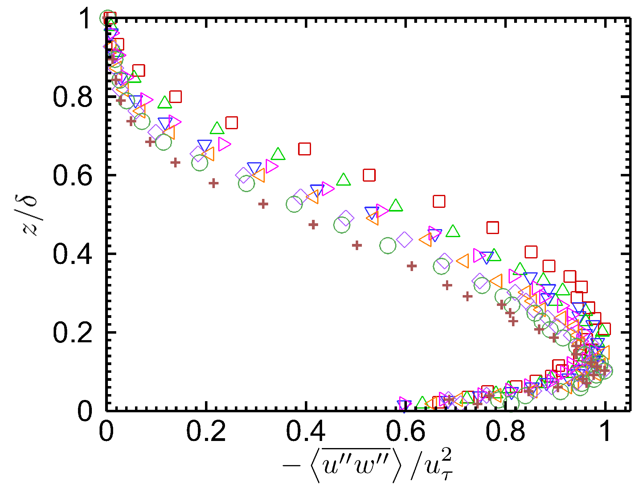
Figure 6.
Shaded contours of joint probability density function (JPDF) and contours of covariance integrand at roof level = over street canyons of hypothetical urban areas of AR = (a) 1:2 and (b) 1:12.
Figure 6.
Shaded contours of joint probability density function (JPDF) and contours of covariance integrand at roof level = over street canyons of hypothetical urban areas of AR = (a) 1:2 and (b) 1:12.

Figure 7.
Frequency spectra of dimensionless streamwise and vertical turbulence intensities at roof level = over building roof (red) and street canyon center (green) over street canyons of hypothetical urban areas of AR = (a) 1:2 and (b) 1:12.
Figure 7.
Frequency spectra of dimensionless streamwise and vertical turbulence intensities at roof level = over building roof (red) and street canyon center (green) over street canyons of hypothetical urban areas of AR = (a) 1:2 and (b) 1:12.


Table 1.
Configuration of the idealized urban surfaces and the flows in the wind tunnel experiments.
Table 1.
Configuration of the idealized urban surfaces and the flows in the wind tunnel experiments.
| Types of Idealized Urban Surface | |||||||||
|---|---|---|---|---|---|---|---|---|---|
| A | B | C | D | E | F | G | H | ||
| Rib [mm] | Size h | 19 | 19 | 19 | 19 | 19 | 19 | 19 | 19 |
| Separation b | 38 | 57 | 76 | 95 | 114 | 152 | 190 | 228 | |
| Size of a repeating unit l (= h + b) [mm] | 57 | 76 | 95 | 114 | 133 | 171 | 209 | 247 | |
| Aspect ratio (= ) | 1:2 | 1:3 | 1:4 | 1:5 | 1:6 | 1:8 | 1:10 | 1:12 | |
| Boundary layer thickness | [mm] | 244 | 248 | 283 | 284 | 294 | 294 | 304 | 304 |
| Sampling location | [mm] | 3705 | 3686 | 3609 | 3648 | 3590 | 3562 | 3571 | 3619 |
| 195 | 194 | 190 | 192 | 189 | 187 | 188 | 190 | ||
| Number of profiles in a repeating unit | 7 | 7 | 7 | 7 | 7 | 9 | 9 | 9 | |
| Velocity [m s] | Free-stream | ||||||||
| Mean | |||||||||
| Friction velocity | [m s] | ||||||||
| Drag coefficient f (= ) [] | |||||||||
| Reynolds number | (= ) | 195,168 | 207,495 | 239,729 | 242,190 | 250,614 | 247,520 | 276,800 | 278,400 |
| (= ) | 15,200 | 15,900 | 16,100 | 16,200 | 16,200 | 16,000 | 17,300 | 17,400 | |
| (= ) | 12,500 | 13,100 | 13,800 | 13,900 | 14,100 | 14,000 | 15,500 | 15,600 | |
| (= ) | 864 | 983 | 1060 | 1127 | 1138 | 1138 | 1229 | 1277 | |
Table 2.
Quadrants for vertical turbulent momentum flux .
| Quadrants | Events | ||
|---|---|---|---|
| 1 | Outward interaction | + | + |
| 2 | Ejection | − | + |
| 3 | Inward interaction | − | − |
| 4 | Sweep | + | − |
© 2017 by the authors. Licensee MDPI, Basel, Switzerland. This article is an open access article distributed under the terms and conditions of the Creative Commons Attribution (CC BY) license (http://creativecommons.org/licenses/by/4.0/).
Share and Cite
MDPI and ACS Style
Ho, Y.-K.; Liu, C.-H. Street-Level Ventilation in Hypothetical Urban Areas. Atmosphere 2017, 8, 124. https://doi.org/10.3390/atmos8070124
AMA Style
Ho Y-K, Liu C-H. Street-Level Ventilation in Hypothetical Urban Areas. Atmosphere. 2017; 8(7):124. https://doi.org/10.3390/atmos8070124
Chicago/Turabian StyleHo, Yat-Kiu, and Chun-Ho Liu. 2017. "Street-Level Ventilation in Hypothetical Urban Areas" Atmosphere 8, no. 7: 124. https://doi.org/10.3390/atmos8070124
Note that from the first issue of 2016, this journal uses article numbers instead of page numbers. See further details here.