An Alternative Estimate of Potential Predictability on the Madden–Julian Oscillation Phase Space Using S2S Models

Abstract

This study proposes an alternative method to estimate the potential predictability without assuming the perfect model. A theoretical consideration relates a maximum possible value of the initial-value error to the covariance between analysis and bias-corrected ensemble-mean forecast. To test the method, the prediction limit of the Madden–Julian Oscillation (MJO) was evaluated, based on three pairs of reanalysis and forecast datasets provided by the European Centre for Medium-Range Weather Forecasting, the Japan Meteorological Agency and the National Centers for Environmental Prediction, participating in the subseasonal-to-seasonal prediction project. The results showed that the predictability was higher when MJO amplitude exceeded unity, consistent with the conventional method in which the error is evaluated as the ensemble-forecast spread. Moreover, the multimodel analysis was also conducted because the proposed method is readily applicable to the multimodel average of ensemble-mean forecasts. The phase dependency of the MJO’s potential predictability is also discussed.

1. Introduction

The Madden–Julian Oscillation (MJO) is dominant intraseasonal variability in the tropics [1,2]. Typically, the convective center of an MJO event is formed over the Indian Ocean, propagates eastward at an average speed of ~5 m s⁻¹ and dissipates in the region between Maritime Continent and the central Pacific. Because of its regular behavior, the MJO is expected to be potentially predictable for 3 weeks or longer [3]. Most operational general circulation models (GCMs) have succeeded to forecast the planetary-scale phenomena related to the MJO for 2–3 weeks [4,5], although they are not capable of an accurate simulation of finer-scale aspects of MJOs such as precipitation distribution [6].

Dynamical MJO forecast has been evaluated as two aspects: prediction skill and potential predictability. The prediction skill on the MJO phase space, meaning model accuracy against the insufficient representation of the MJO, has been gradually increased. Rashid et al. [7] found that the MJO could be predicted for 21 days in an Australian GCM measured with a bivariate correlation coefficient (e.g., [8]). A new-generation cloud-resolving model also successfully predicted several MJO events [9]. The monthly forecasts operated by the European Centre for Medium-Range Weather Forecasts (ECMWF) furthermore improved the skill to nearly a month for any initial MJO phases [10]. On the other hand, the potential predictability, representing the intrinsic uncertainty due to the chaotic nature of the atmosphere, was usually estimated from a single-model ensemble forecast by calculating spread among members involved with a small initial perturbation. However, because most of the GCMs could not sustain the convective activity of MJO, the ensemble members tended to dump into the origin of MJO phase space. Waliser et al. [3] focused on this dumping problem and estimated the intrinsic limit of predictability as the forecast lead time at which spread multiplied by $\sqrt{2}$ attains the MJO amplitude. Their estimate was about 25–30 days for 200 hPa velocity potential. Neena et al. [5], applying the same method to each of eight GCMs, estimated that the potential predictability is 20–30 days in the MJO phase space. They also found the dependence of predictability on the initial phase of the MJO. In spite of a similar metric in an ensemble forecast analysis, Kim et al. [11] suggested that the potential predictability was insensitive to the initial MJO phase.

We now caution that all the above studies on the potential predictability implicitly assumed that a forecast model perfectly represented the MJO time-series in their estimates. However, the perfect-model assumption is not always reasonable for the MJO prediction, because most GCMs still underestimate the MJO amplitude and then distort the climatological probability distribution in the MJO phase space [6,10,12,13]. If we developed an alternative approach to evaluate the potential predictability without the perfect-model assumption, we could extricate ourselves from model dependence in the estimation. The theoretical consideration by Kumar and Hoerling [14] may help us relate the magnitude of the initial-value error to the statistics of analysis and imperfect-model forecast data. If one removed the model bias averaged over the forecasts [15], the potential predictability would be related to the manner in how the forecasts are covariated with the analyses, as will be discussed later [16,17,18]. Recently, the sub-seasonal to seasonal (S2S) prediction project has been launched and posed the MJO forecast as one of the most important targets [19,20,21]. We can access a set of hindcasts with operational GCMs, each of which has different resolution and physical parameterizations. A model estimate of potential predictability has not been established yet, because the perfect-model assumption obstructs a reasonable compilation of results. Hence a new approach without the perfect-model assumption would be applicable to multimodel ensemble analysis.

The purpose of this study is to propose an alternative method to estimate the potential predictability without assuming the perfect model, which is completely different from a conventional method to evaluate the spread of initial perturbations in an ensemble forecast. The point of this paper is the strategy to cope with an averaged time-series over the ensemble members, posing the analysis time-series as its counterpart. A set of analyses and forecasts projected onto the MJO phase space starting from various dates are then prepared. In order to achieve this purpose, we first formulate the estimation method of potential predictability based on a set of analyses and forecasts. The method newly developed in this paper is capable of being applied to multimodel ensemble analysis. The rest of the paper is organized as follows. Section 2 gives the description on analysis and forecast data that we used here. The MJO phase space is also defined. Section 3 develops an alternative method to estimate potential predictability. Section 4 compares the new method with a conventional method, and then the new method is applied to multimodel ensemble analysis. Concluding remarks are given in Section 5.

2. Data

2.1. Verification and Phase Space

The verification in this paper is an average of ERA-Interim of ECMWF [22], JRA55 of the Japan Meteorological Agency (JMA; [23]), and the Climate Forecast System (CFS) reanalysis version 2 from the National Centers for Environmental Prediction (NCEP; [24]). Presumably because of the sparseness of surface observation and the deficit of model parameterizations, a discrepancy among reanalyses is not negligible in the tropics [25,26]. While most previous works evaluated GCMs’ performance with their own reanalysis as the verification, the reanalysis average enabled us to fairly compare the prediction among models [27], which was expected to provide a more optimal estimate than a single analysis [28].

The MJO phase space is spanned by two gravest combined empirical orthogonal function (EOF) modes of zonal wind at 200 hPa and 850 hPa, averaged between 15° S and 15° N based on NCEP’s CFS (Climate Forecast System) reanalysis version 2 from 1979 to 2015 [29]. If the data were replaced with the reanalysis average, the MJO phase space changed little. We excluded the outgoing longwave radiation data from the combined EOF analysis for simplicity, as the two gravest EOF modes with outgoing longwave radiation and zonal winds have little difference from those with zonal winds only [4,30]. Climatology and the 120-day average were removed from zonal wind prior to the EOF analysis to extract the intraseasonal variations, and the signal of the El Niño/Southern Oscillation was automatically removed in this processing [8]. We classified the MJO phase as conventional and the non-MJO phase was defined as the state where the MJO amplitude is less than unity.

2.2. Forecast Data

We used reforecast data with three GCMs joining the S2S project (http://s2sprediction.net/): operational models of ECMWF [10], GSM1403C of the JMA [31] and CFS version 2 of NCEP [32]. The details are provided in

Table 1. Subeasonal-to-seasonal (S2S) forecast models selected in this model.

Organization	ECMWF	JMA	NCEP
Forecast period	32 days	33 days	44 days
Initial perturbation	Singular vector and ensemble data assimilation perturbation	Bred vector and lagged averaging method	Lagged averaging method
Ensemble size	4	4	3
Initial time	00 UTC	12 UTC	00 UTC
Frequency	Twice a week	3 times a month	Everyday
Total number of forecasts	1397	396	3972
Horizontal resolution	TL639 (TL319 after day 10)	TL319	T126
Vertical layers	91	60	64

ECMWF: the European Centre for Medium-Range Weather Forecasts; JMA: the Japan Meteorological Agency; NCEP: the National Centers for Environmental Prediction.

. Hereafter, each model is called by the name of its organization (e.g., the JMA model for GSM1403). The data period is from January 1999 to December 2009. Model forecast data were also projected on the phase space, after a removal of the seasonality and 120-day average using the reanalysis provided with the corresponding model. In S2S reforecast data, an initial perturbation was created using singular vector and ensemble data assimilation perturbation by ECMWF, using the bred vector and lagged averaging (LAF) method by the JMA, and using the LAF method for NCEP.

A stumbling block when using the reforecast data joining the S2S project is a different interval of initial date and time, which makes it difficult to find a set of models initialized on the same date. The ECMWF model has 1397 forecasts that were initialized at 00 UTC of the calendar date, corresponding to Thursdays between January 2015 and May 2016, or Mondays from 14 May 2015 to 30 May 2016. The JMA model has 396 forecasts that ran from 12 UTC of the 10th, 20th and the last day of each month. The NCEP model has 3972 forecasts beginning from 00 UTC of every date during the period. For the multimodel ensemble forecast analysis, ECMWF, JMA and NCAR reforecasts were selected only if the difference of initial time is less than 12 h; for example, the JMA model’s reforecast, initialized on the 20th of March at 12 UTC, was grouped in the multimodel analysis with the ECMWF and NCEP models’ reforecasts, which were initialized on the 21st of March at 00 UTC. This selection was effective in matching the initial date among the forecasts, and we realized multimodel ensemble analysis with 250 independent forecasts. The list of calendar dates is provided in

Table 2. A list of months and days on which the multimodel ensemble analysis was performed between 1999 and 2009.

Month	Day
Jan.	1	11	21
Feb.	1	11
Mar.	10	21	31
Apr.	11	21	30
May	21
Jun.	11
Jul.	20
Aug.	10	20	31
Sep.	10	21
Oct.	1
Nov.	30
Dec.	10	21

, and the number of single model and multimodel forecasts initialized in each MJO phase are shown in

Table 3. The number of individual forecasts, each with its own forecast period, starting from each piecewise area in the Madden–Julian Oscillation (MJO) phase space.

Phase Block	ECMWF	JMA	NCEP	Multimodel Ensemble
Non-MJO phase	570	160	1661	107
All MJO phase	827	236	2311	143
Phases 2–3	182	51	511	41
Phases 4–5	218	64	638	43
Phases 6–7	196	58	529	31
Phases 8–1	231	63	633	28

. It is noted that the forecasts initialized on 1 January 1999, 1 February 2003 and 11 February 2003 were excluded for a technical reason.

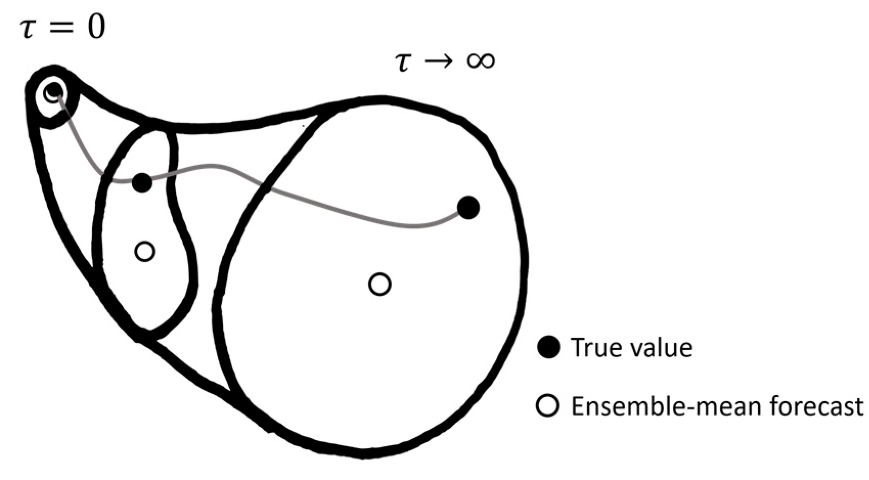
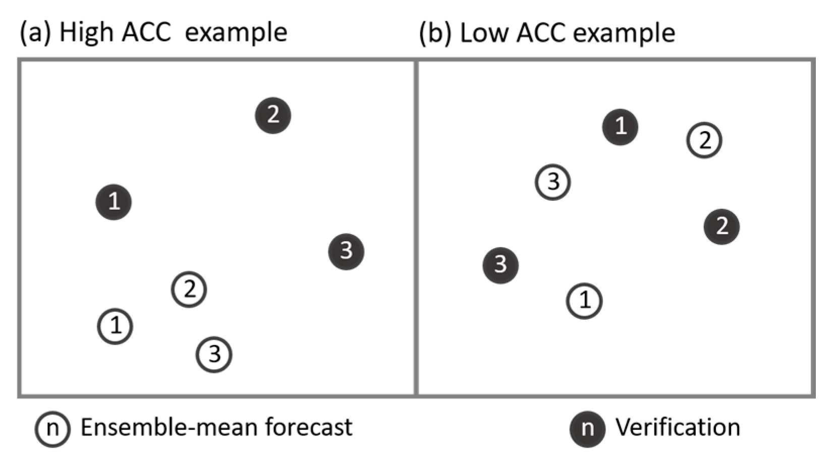
3. Alternative Method to Estimate Potential Predictability

Consider the time-series of the true value, ${\mathit{X}}^{\mathit{o}}$, and the perfect model hypothetically (Figure 1). We first clip a part of the time-series ${\mathit{X}}^{\mathit{o}}$ in the range from $t_0$ to $t_0+T$, and the time segment is renamed as ${\mathit{X}}_{\mathbf{1}}^{\mathit{o}}\left(\tau \right)$ for $0\le \tau \le T$. We numbered the time segment (see below) in the subscript. The superscripts o, f and e mean the truth, the ensemble mean and the initial-value error, respectively, almost following the notation of data assimilation [33]. The perfect model, as a thought experiment, would be repeatedly integrated from ${\mathit{X}}_{\mathbf{1}}^{\mathit{o}}\left(0\right)$ plus an initial error, the magnitude of which is infinitesimally small and randomly given. Taking an average over infinite ensemble members of the above experiment, we can obtain the time segments of the ensemble mean perfect-model forecast written as ${\mathit{X}}_{\mathbf{1}}^{\mathit{f}}$ here. We now emphasize that the nonlinearity intrinsic to the system causes the difference between ${\mathit{X}}_{\mathbf{1}}^{\mathit{o}}$ and ${\mathit{X}}_{\mathbf{1}}^{\mathit{f}}$ for $\tau >0$. This difference, expanding in time, is regarded as the initial-value error ${\mathit{X}}_{\mathbf{1}}^{\mathit{e}}\left(\tau \right)={\mathit{X}}_{\mathbf{1}}^{\mathit{o}}\left(\tau \right)-{\mathit{X}}_{\mathbf{1}}^{\mathit{f}}\left(\tau \right)$. As $\tau$ approaches infinity, the ensemble members of the perfect model scatter over the phase space following the climatological probability density function (PDF) of the true value. The ensemble-mean ${\mathit{X}}_{\mathbf{1}}^{\mathit{f}}\left(\tau \right)$ is asymptotic to the origin of the phase space, while the true value ${\mathit{X}}_{\mathbf{1}}^{\mathit{o}}\left(\tau \right)$ is not converged to a certain value as $\tau \to \infty$.

Next, we labeled a set of time segments of the true value as

$$\left\{{\mathit{X}}_{\mathbf{1}}^{\mathit{o}}\left(\tau \right), {\mathit{X}}_{\mathbf{2}}^{\mathit{o}}\left(\tau \right),\dots ,{\mathit{X}}_{\mathit{N}}^{\mathit{o}}\left(\tau \right)\right\}$$

(1)

and that of corresponding ensemble-mean forecasts as

$$\left\{{\mathit{X}}_{\mathbf{1}}^{\mathit{f}}\left(\tau \right), {\mathit{X}}_{\mathbf{2}}^{\mathit{f}}\left(\tau \right),\dots ,{\mathit{X}}_{\mathit{N}}^{\mathit{f}}\left(\tau \right)\right\}$$

(2)

where N is the total number of selected time segments. As ${\mathit{X}}_{\mathit{j}}^{\mathit{f}}\left(\tau \right)$ is uncorrelated with the initial-value error ${\mathit{X}}_{\mathit{j}}^{\mathit{e}}\left(\tau \right)$ for all time segments $1\le \mathit{j}\le N$, the variance of the true values among a set of time segments Equation (1), ${\sigma }^2\left[{\mathit{X}}^{\mathit{o}}\left(\tau \right)\right]$, can be represented by the variance of the ensemble-mean forecasts among a set of time segments Equation (2), ${\sigma }^2\left[{\mathit{X}}^{\mathit{f}}\left(\tau \right)\right]$, added by the initial-value error spread [16,34,35]:

$${\sigma }^2\left[{\mathit{X}}^{\mathit{o}}\left(\tau \right)\right]={\sigma }^2\left[{\mathit{X}}^{\mathit{f}}\left(\tau \right)\right]+{\sigma }^2\left[{\mathit{X}}^{\mathit{e}}\left(\tau \right)\right]$$

(3)

At $\tau =0$, ${\sigma }^2\left({\mathit{X}}^{\mathit{o}}\right)$ is equal to ${\sigma }^2\left({\mathit{X}}^{\mathit{f}}\right)$ as the initial-value error should be zero. As $\tau$ approaches infinity, ${\sigma }^2\left({\mathit{X}}^{\mathit{o}}\right)$ becomes the variance of climatological probability density function (PDF). For this limit, since ${\mathit{X}}_{\mathit{j}}^{\mathit{f}}\to \mathbf{0}$ for all time segments $\mathit{j}$, the variance is exactly zero. Now we introduce the anomaly correlation coefficient (ACC) between the true value and ensemble-mean forecast as

$$r=\frac{1}{N-1}{\displaystyle \sum }_{j=1}^N\frac{({\mathit{X}}_{\mathit{j}}^{\mathit{o}}-⟨{\mathit{X}}^{\mathit{o}}⟩)\cdot ({\mathit{X}}_{\mathit{j}}^{\mathit{f}}-⟨{\mathit{X}}^{\mathit{f}}⟩)}{\sigma ({\mathit{X}}^{\mathit{o}}) \sigma ({\mathit{X}}^{\mathit{f}})}$$

(4)

where the angle bracket denotes the average over the time segments. The ACC is high if the true value is well covariated with the forecast (Figure 2a); otherwise, it is low (Figure 2b). By using the relation ${\mathit{X}}_{\mathit{j}}^{\mathit{o}}\left(\tau \right)={\mathit{X}}_{\mathit{j}}^{\mathit{f}}\left(\tau \right)+{\mathit{X}}_{\mathit{j}}^{\mathit{e}}\left(\tau \right)$ and the independence between ${\mathit{X}}_{\mathit{j}}^{\mathit{f}}\left(\tau \right)$ and ${\mathit{X}}_{\mathit{i}}^{\mathit{f}}\left(\tau \right)$, the ACC is reduced to the ratio of the standard deviation of the forecast to that of the true value:

$$r=\frac{\sigma \left({\mathit{X}}^{\mathit{f}}\right)}{\sigma \left({\mathit{X}}^{\mathit{o}}\right)}$$

(5)

Finally, we arrive at the hypothesis that ${\mathit{X}}_{\mathit{j}}^{\mathit{f}}$ would be created with the perfect model. If ${\mathit{X}}^{\mathit{f}}$ is reconsidered to be the ensemble-mean of an imperfect model forecast, we add one extra term of covariance between forecast and error, $C\left({\mathit{X}}^{\mathit{f}},{\mathit{X}}^{\mathit{e}}\right)$, as

$$r^{ }=\frac{\sigma \left({\mathit{X}}^{\mathit{f}}\right)}{\sigma \left({\mathit{X}}^{\mathit{o}}\right)}+\frac{C\left({\mathit{X}}^{\mathit{f}},{\mathit{X}}^{\mathit{e}}\right)}{\sigma \left({\mathit{X}}^{\mathit{o}}\right)\sigma \left({\mathit{X}}^{\mathit{f}}\right)}$$

(6)

Because the initial-value error deteriorates the forecast, the extra cross-correlation term is, in general, negative. Therefore, the equality in Equation (6) is replaced with the inequality as below [18]:

$$r^{ }\le \frac{\sigma \left({\mathit{X}}^{\mathit{f}}\right)}{\sigma \left({\mathit{X}}^{\mathit{o}}\right)}$$

(7)

The ACC is unity at the initial time and almost monotonically decreases with the lead time. Within the range of a positive ACC, using Equation (3), we can derive the inequality that determines a possible maximum value of initial-value error based on a set of time segments of the true value and the ensemble-mean forecasts as

$$\sigma \left({\mathit{X}}^{\mathit{e}}\right)\le \sigma \left({\mathit{X}}^{\mathit{o}}\right)\sqrt{1-r^2}$$

(8)

The prediction limit should be evaluated as the time when $\sigma \left({\mathit{X}}^{\mathit{o}}\right)\sqrt{1-r^2}$ reaches a threshold value. On the MJO phase space, we used the threshold value of unity, that is, about 70 percent of the climatological variance. It is worthwhile remarking that the new method only uses the ensemble-mean forecast data and does not use each ensemble member like the conventional method. Expanding Equation (8) to multi-model analysis with M models, the inequality should be $\sigma \left({\mathit{X}}^{\mathit{e}}\right)\le \sigma \left({\mathit{X}}^{\mathit{o}}\right)\sqrt{1-R^2}$. Here, $R$ is the maximum ACC among the models and their mean, because our evaluation only provides the lower bound of predictability.

For a practical use of the above theoretical consideration in this paper, we replaced the true value with verification defined in Section 2, the reanalysis average. Even so, the discrepancy in the initial state between verification and ensemble-mean forecast was not negligible. We hence constantly offset the time segment of forecast ${\mathit{X}}_{\mathit{j}}^{\mathit{f}}\left(\tau \right)$, so as to match its initial state ${\mathit{X}}_{\mathit{f}}^{\mathit{j}}\left(0\right)$ with the verification ${\mathit{X}}_{\mathit{j}}^{\mathit{o}}\left(0\right)$ for each time segment:

$${\tilde{\mathit{X}}}_{\mathit{j}}^{\mathit{f}}\left(\tau \right)={\mathit{X}}_{\mathit{j}}^{\mathit{f}}\left(\tau \right)-\left({\mathit{X}}^{\mathit{f}}\left(0\right)-{\mathit{X}}^{\mathit{o}}\left(0\right)\right)$$

(9)

Moreover, the bias correction is made, the details of which will be explained in the next section. Since we focus on the MJO behavior, ${\mathit{X}}^{\mathit{o}}$ and ${\mathit{X}}^{\mathit{f}}$ are hereafter two-dimensional vectors on the MJO phase space.

It is cautioned that the ACC is different from the bivariate correlation coefficient (BCC) that was often used for the evaluation of prediction skill on the MJO phase space [15]:

$$\rho =\frac{1}{N-1}{\displaystyle \sum }_{j=1}^N\frac{{\mathit{X}}_{\mathit{j}}^{\mathit{o}}\cdot {\mathit{X}}_{\mathit{j}}^{\mathit{f}}}{s\left({\mathit{X}}^{\mathit{o}}\right) s\left({\mathit{X}}^{\mathit{f}}\right)}$$

(10)

where $s\left(\mathit{X}\right)$ is mean amplitude $\sqrt{1/N{\sum }_{j=1}^N{\left|{\mathit{X}}_{\mathit{j}}\right|}^2}$. The BCC is formerly related to the ACC as

$$\rho =r+\frac{1}{N-1}{\displaystyle \sum }_{j=1}^N\frac{⟨{\mathit{X}}^{\mathit{o}}⟩\cdot ⟨{\mathit{X}}^{\mathit{f}}⟩}{s\left({\mathit{X}}^{\mathit{o}}\right) s\left({\mathit{X}}^{\mathit{f}}\right)}$$

(11)

only when the lead time is sufficiently large so that $\sigma \left(\mathit{X}\right)=s\left(\mathit{X}\right)$. Now, as we evaluate the predictability for forecasts initialized on some blocks of the MJO phase space, the mean of state is generally non-zero. Hence, the BCC cannot simply be relevant to the initial-value error in the way described in our formulation.

4. Results

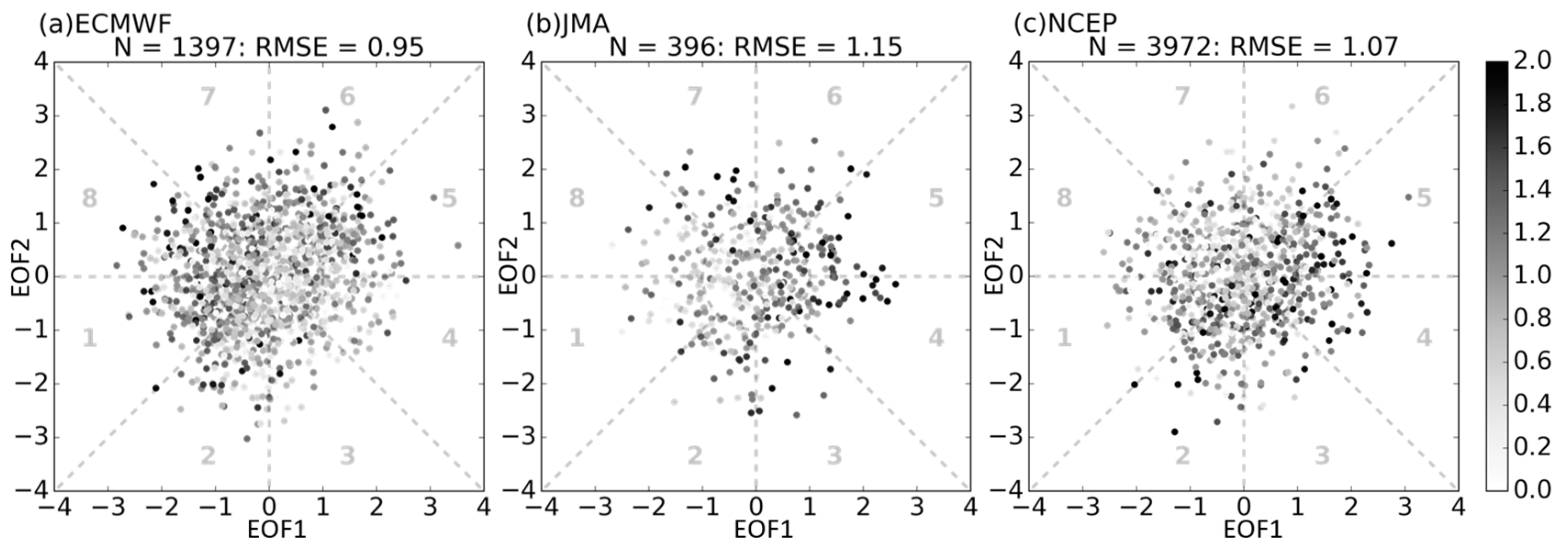
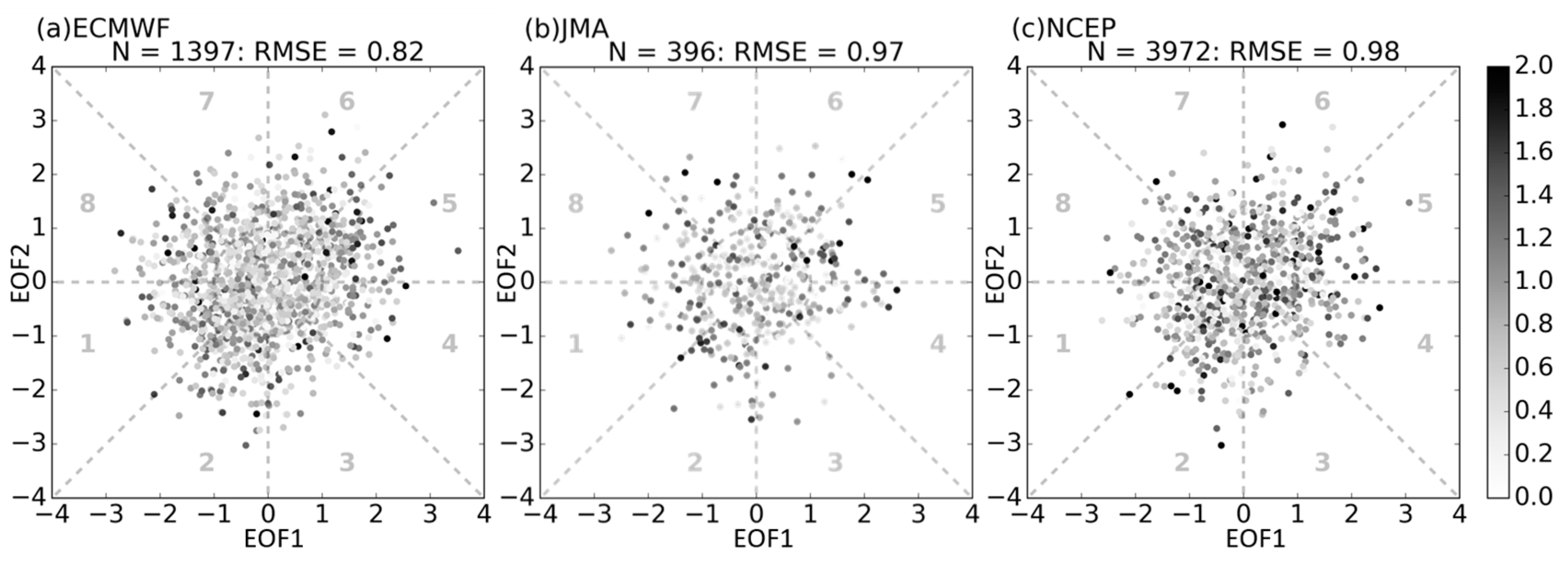
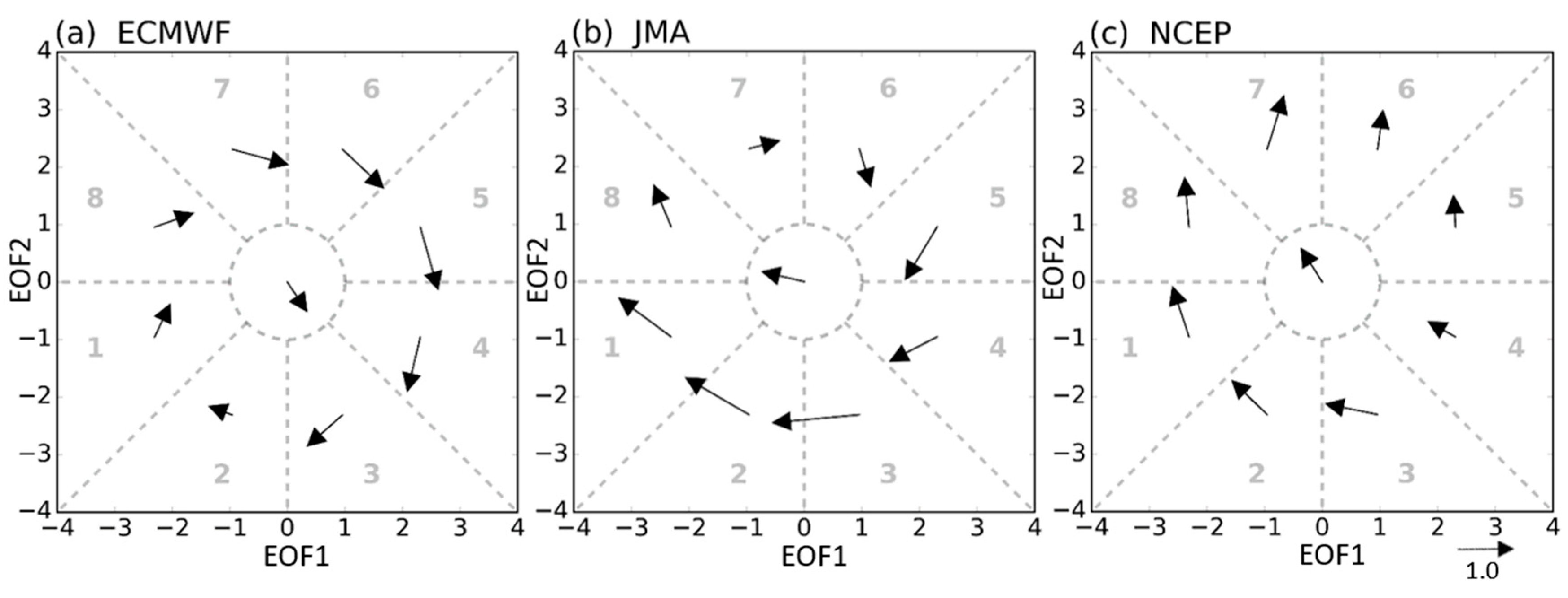
4.1. The Prediction Skill and Bias Correction

This section shows the predictability estimated with the new method developed in the above section, which provides a maximum possible value of initial-value error based on a pair of analysis and ensemble-mean forecast datasets. To effectively test the new method, it is better to remove the model bias from the forecast data in advance. Hence, we first discuss the prediction skill for each model, and then make the bias correction by removing the bias vector averaged over each MJO phase. The prediction skill is now evaluated as the distance between ensemble-mean forecast state and the analysis state on the MJO phase space, defined as the two gravest combined-EOF modes of tropical zonal wind. Each separated block in the figures of this paper corresponds to the MJO phase: the convective center is located over the Indian Ocean in Phases 2–3, the Maritime Continent in Phases 4–5 and the western Pacific in Phases 6–7, while Phases 8–1 correspond to suppressed or formation stages. Figure 3 displays the prediction skill at 10-day lead time calculated for each forecast as the dot plot at the initial-state position on the MJO phase space, with the root-mean-square error (RMSE) as the statistics among forecasts. The best-performing model was ECMWF’s, with the RMSE less than unity at this lead time. The RMSE was 1.07 for the NCEP model and 1.15 for JMA’s. The two models (Figure 3b,c) especially provided erroneous forecasts with the RMSE exceeding 1.4 when initialized in Phases 4–5, in which convection is active over the Maritime Continent. Contrastingly, the ECMWF model predicted the MJO state more accurately when initialized there, while it provided erroneous forecasts initialized in Phases 8–2, in which the signal resides between Africa and the central Indian Ocean.

The model bias as a function of lead time was defined for each initial phase as the bias vector averaged over the forecasts starting from a phase (Figure 4). The bias vector at 10-day lead time in the JMA model showed a clockwise tendency with a leftward translation over the phase space (Figure 4b), moderately consistent with Ichikawa and Inatsu [15]. The bias vector in the NCEP model showed a tendency toward the positive direction of the second principal component with a weak clockwise motion (Figure 4c). The bias vector of ECMWF was characterized by clockwise rotation uniformly over the space, corresponding to a bias of slower eastward propagation of the MJO convective center (Figure 4a). The bias correction was made for each model forecast by subtracting the bias vector shown in Figure 4 from the original forecast state vector. Figure 5 shows the error plot after making a bias correction. The bias correction made the error phase-independent in all three models. The RMSE decreased by 0.1 for the ECMWF and NCEP models (Figure 5a,c). In the JMA model, the RMSE dropped from 1.15 to 0.97 as a result of the effective bias correction (Figure 5b).

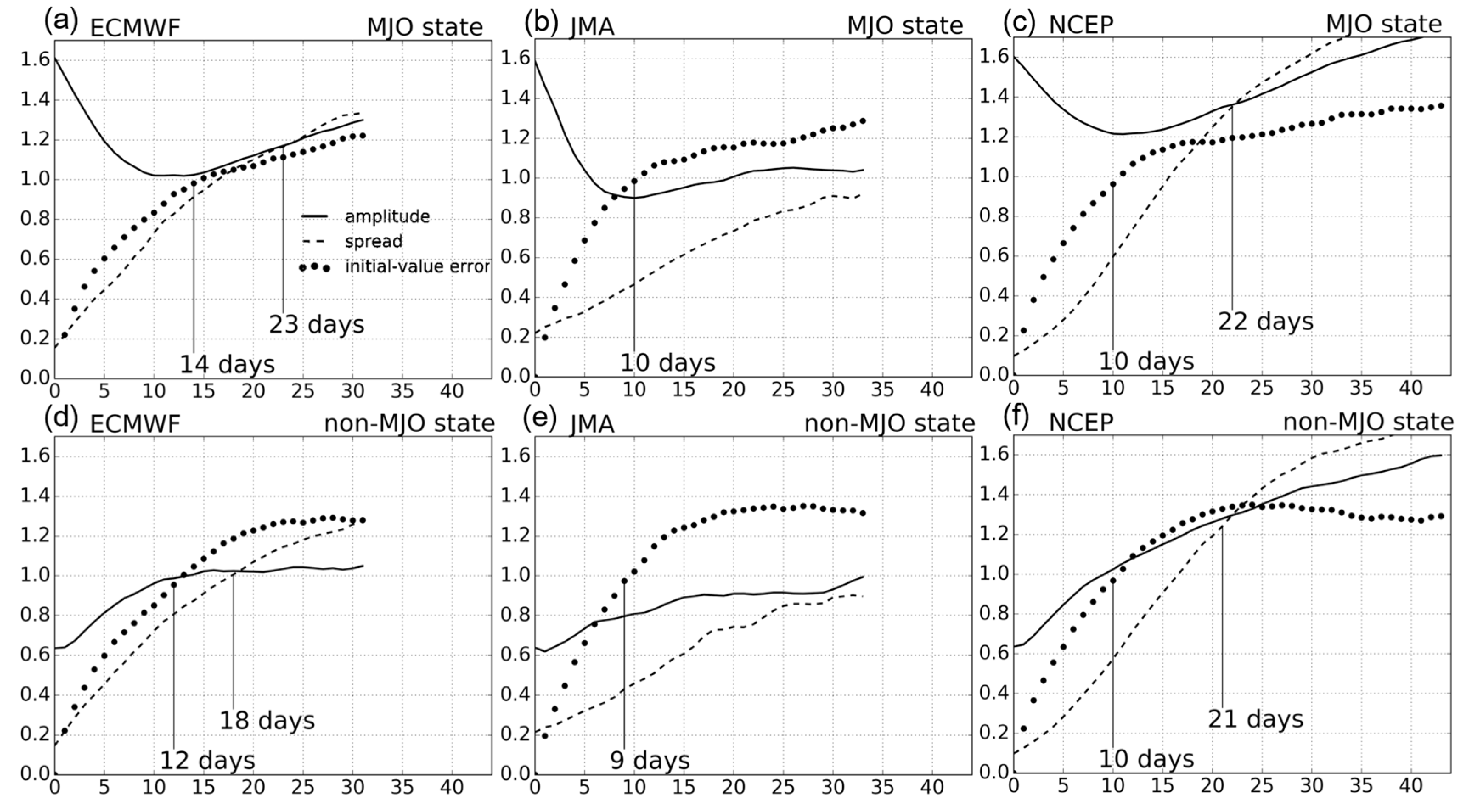
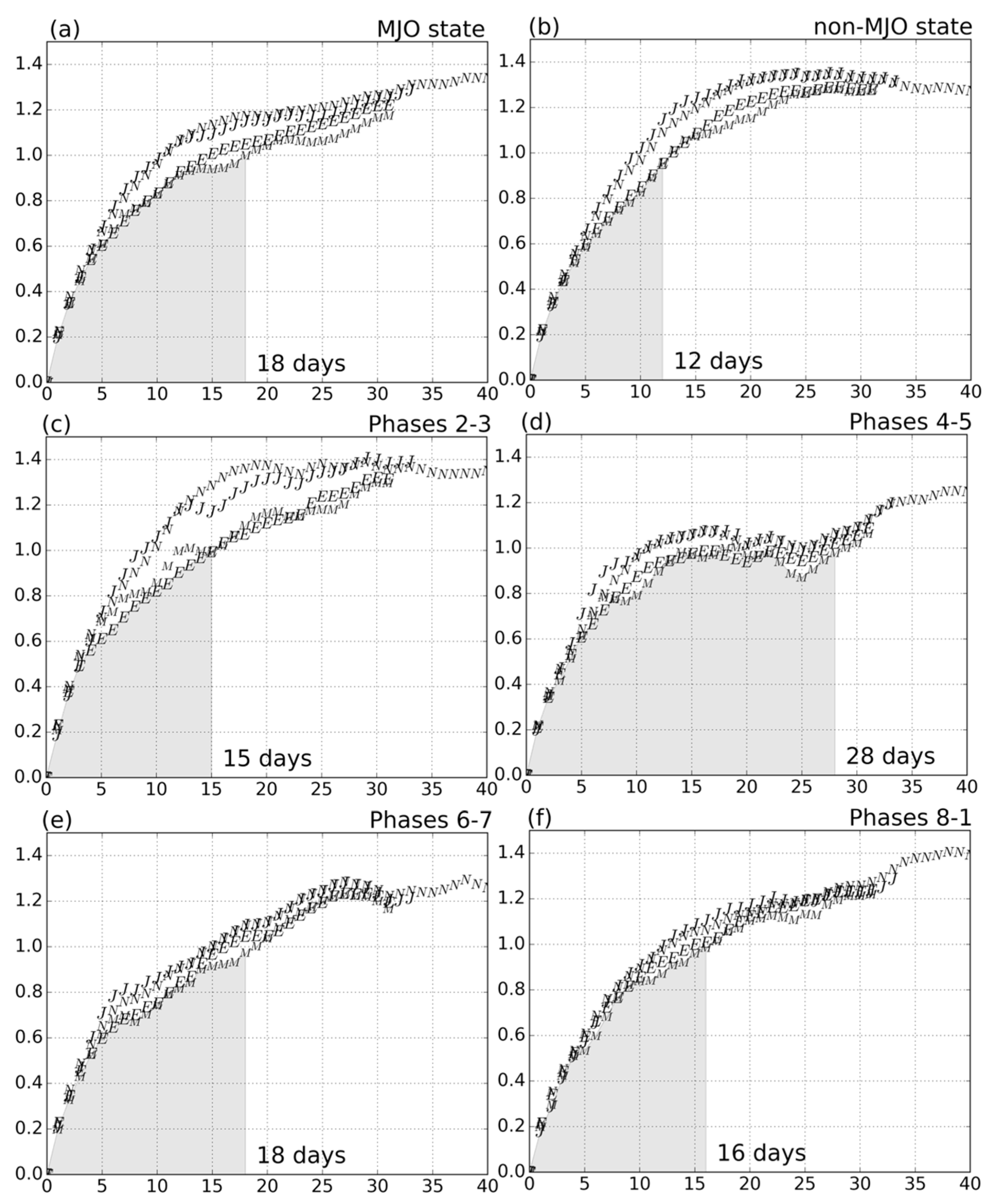
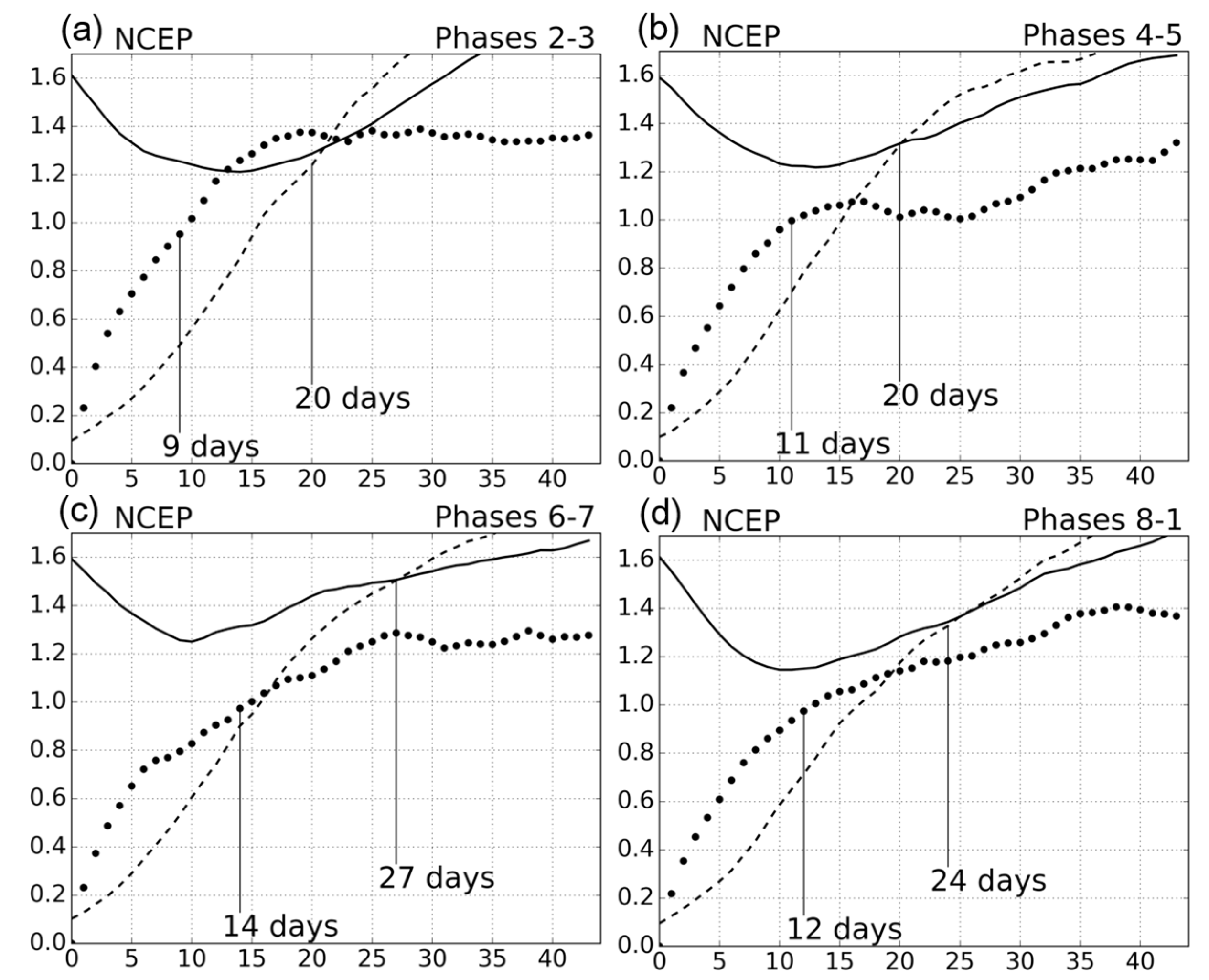
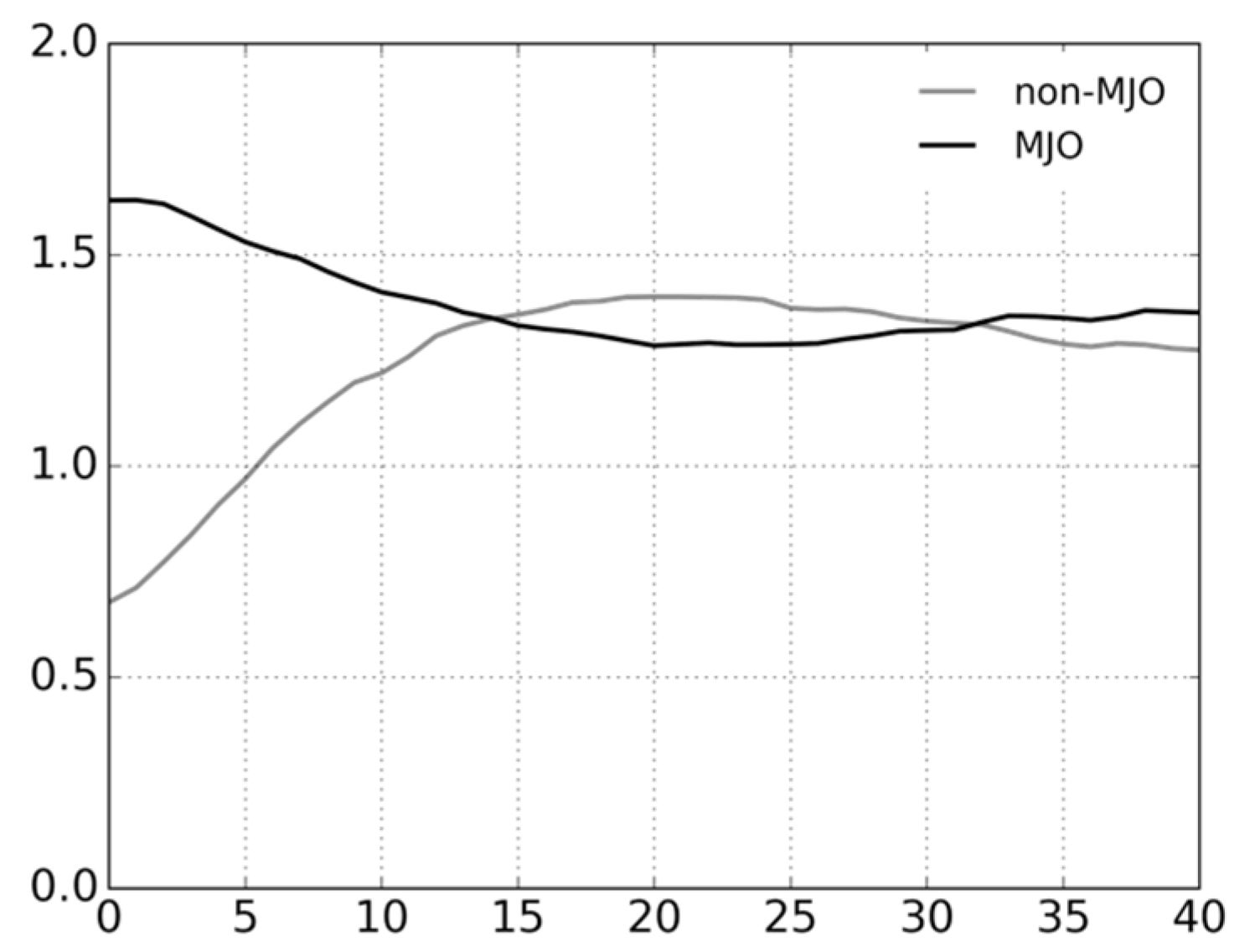
4.2. Prediction Limit and Its Comparison with a Conventional Method

Predictability was evaluated with prediction limit in this paper. The proposed method provided a maximum-possible value of initial-value error variance as a function of the lead time. Therefore, it provided a minimum-possible value of the prediction limit defined as the lead day just before the initial-value error variance attains unity, accounting for half the climatological variance of the data on the 2-dimensional phase space. As the time goes to infinity, the variance of analysis time segments is asymptotic to 2. The new method, in essence, evaluates the prediction limit when a possible maximum of initial-value error multiplied by $\sqrt{2}$ reaches this limitation. This is analogous to the conventional method in which the prediction limit is defined as the time when the ensemble spread multiplied by $\sqrt{2}$ reaches the MJO amplitude. It is worthwhile noting that $\sigma \left({\mathit{X}}^{\mathit{o}}\right)\to \sqrt{2}$ can be used in the new method but the spread goes to the MJO amplitude in the limit due to the model’s imperfectness [5]. In order to be fairly compared with the method proposed in this paper, the prediction limit was evaluated following Neena et al. [5], except that we did not take a 51-day running average for amplitude due to the limited length of prediction. As the new method gives the minimum possible value of prediction limit, it can be said that the conventional method provides a fake short limit when it is shorter than the new method estimation.

We first tested the new method in light of the classification of forecasts on the initial MJO amplitude. Averaging over forecasts of which the initial MJO amplitude exceeds unity, a minimum possible value of prediction limit was 14 days based on the ECMWF model and 10 days based on the JMA and NCEP models (Figure 6a–c). In contrast, averaging over forecasts starting from a non-MJO state, the minimum-possible prediction limit was 12 days based on the ECMWF model, 9 days based on JMA’s and 10 days based on NCEP’s (Figure 6d–f), slightly shorter than forecasts from MJO states. This result suggests that the forecasts starting from an MJO state are, on average, more predictable than those starting from a non-MJO state. This is consistent with the consequence from the conventional method. The prediction limit in the ECMWF model was estimated as 23 days for forecasts from an MJO state, while it was 18 days for forecasts from a non-MJO state (Figure 6a,d). Similarly, the prediction limit for the NCEP model was 23 days for an initial MJO state and 21 days for an initial non-MJO state (Figure 6c,e). Although the conventional method did not provide the prediction limit for the JMA model due to no crossing of amplitude and spread lines, the prediction limit seems shorter in forecasts with initial non-MJO states (Figure 6d). This result was not substantially changed even if we classified forecasts by the average MJO amplitude through forecast period, and we found a longer prediction limit for the forecasts for which average amplitude exceeded unity (not shown).

Our method can also be utilized to estimate the dependence of MJO predictability at the initial phase. Here, the results are shown in Figure 7 for the NCEP model and

Table 4. The list of prediction limits for the ECMWF model (day) for forecasts from each MJO phase with the proposed and conventional methods.

Initial State	Proposed Method	Conventional Method
Phases 2–3	15	17
Phases 4–5	27	27
Phases 6–7	16	25
Phases 8–1	14	17

for the ECMWF model. A minimum-possible prediction limit based on the NCEP model was longest for forecasts from Phases 6–7 and shortest for forecasts from Phases 2–3. This phase dependence is coherent with the prediction limit estimated with ensemble spread, and the low prediction limit for forecasts initialized in Phases 2–3 may be due to an irregular amplitude change over the Maritime Continent. The ECMWF model provided a minimum-possible prediction limit at 27 days for forecasts from Phases 4–5, much longer than that for forecasts from other phases. This is likely because there is little possibility to initiate another MJO event under the dry environment that occurs after the MJO passage over the Indian Ocean and the Maritime Continent. This is also in line with the prediction limit estimated with the conventional method, although the difference among phases is not so prominent.

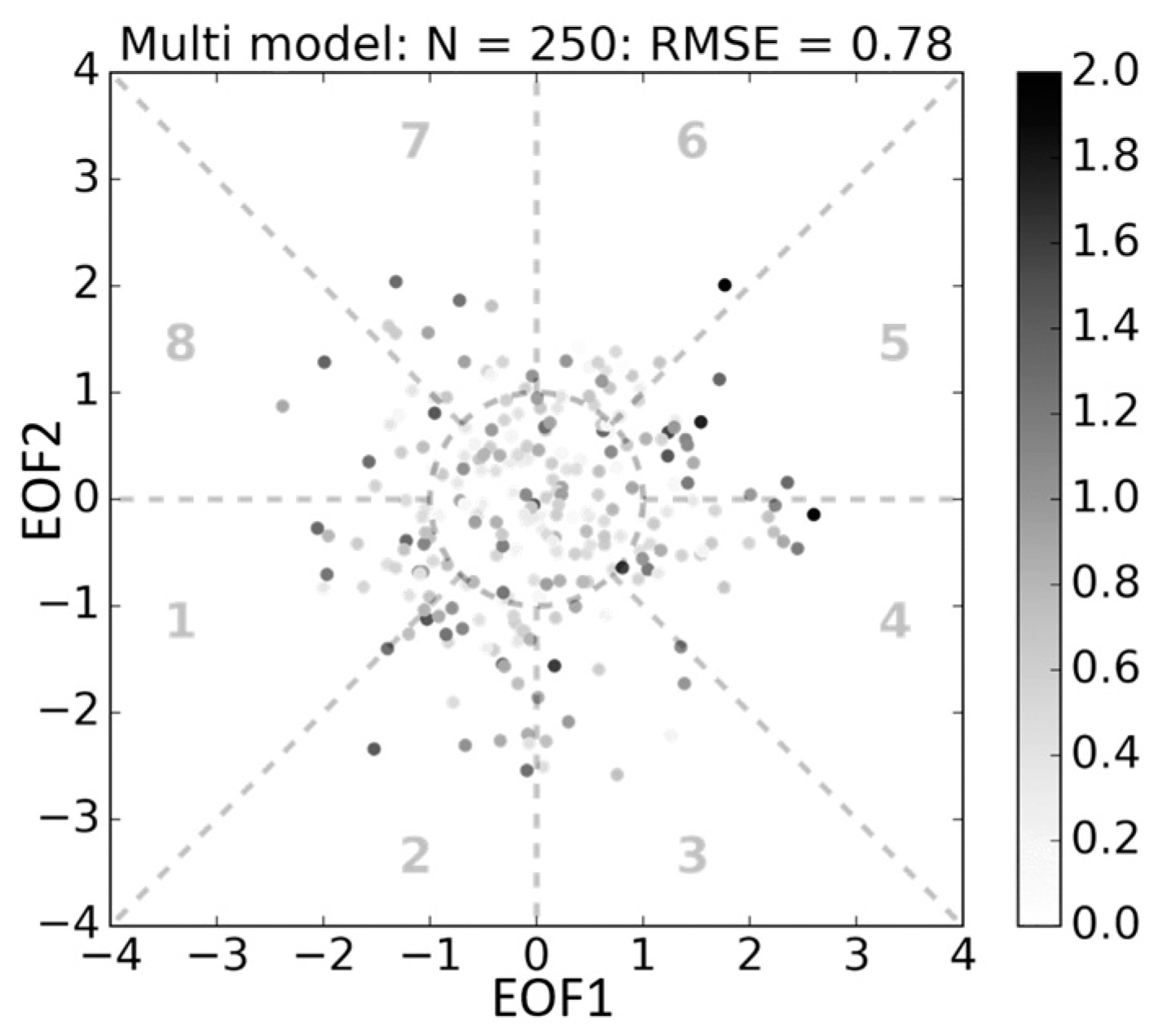
4.3. The Multimodel Ensemble Analysis

The multimodel analysis combined the estimates of prediction limit from each of the single models and the multimodel average. The multimodel average is expected, in general, to provide a better forecast than the single model. Figure 8 shows the prediction skill of forecasts averaged among the ECMWF, JMA and NCEP models after a bias correction. Although the sample number was only 250, as pointed out in section 2, the RMSE was less than any other models’ (Figure 5). Similarly, the multimodel analysis gives a longer estimate of potential predictability than the single model analysis. Considering this point, we now regard the multimodel average as one of the model results, and a minimum-possible prediction limit is defined as the lead day just before the smallest estimate of initial-value error among the models reaches unity, in order to get the longest minimum values possible. The new method can extend to multimodel analysis in this manner, while the conventional method cannot.

A minimum-possible prediction limit in the multimodel analysis is shown in Figure 9. For forecasts of which the initial amplitude exceeded unity, the smallest estimate of initial-value error reached unity at 18 days (Figure 9a). For forecasts starting from a non-MJO state (Figure 9b), in contrast, the minimum-possible prediction limit was 12 days. The multimodel analysis also supports the notion that the potential predictability of forecasts from an MJO state is longer than that from a non-MJO state. Having classified the initial state as in the previous section, we investigated the dependence of the potential predictability on MJO phase in the multimodel analysis. The minimum-possible prediction limit for forecasts initialized in Phases 4–5 was 28 days, while that for forecasts initialized in other phases was 15–18 days. This is because the variance ${\sigma }^2\left({\mathit{X}}_0\right)$ is so small that the initial-value error can keep less than unity even with the relatively low ACC.

It is cautioned that there is an estimation error in the evaluation above caused by the small sample size in the multimodel analysis. For example, there are only 31 and 28 forecasts initialized in Phases 6–7 and Phases 8–1, respectively (Table 3). In these cases, the estimation error of the initial-value error could be as large as ~0.05–0.08 around the lead time when it reaches unity, according to the boot-strap method (not shown).

5. Concluding Remarks

This study has proposed an alternative method to estimate potential predictability without making the perfect model assumption. The formulation started from the definition of the initial-value error as the difference between the analysis and ensemble-mean forecast. Their covariance among a bundle of time segments is a key point in developing the new method. Applying it to the two-dimensional state on the MJO phase space, the potential predictability for three operational models participating in the S2S project was successfully evaluated. The results suggested that forecasts from an MJO state provided a longer prediction limit, on average, than forecasts from a non-MJO state. Our method also detected a longer prediction limit for forecasts initially from Phases 4–5. We obtained consistent results from a conventional method in which the initial-value error was estimated with the spread of ensemble members normalized by the amplitude of the MJO signal. Though we obtained a similar result to the conventional method, our new method has three merits: it can be used for phenomena that are not well forecasted by models; it can be used for multimodel ensemble analysis; and it can identify a fake short prediction limit obtained using the conventional method. Another different point from the conventional method is the use of the ensemble spread. The ensemble members or their spread might have more information than their mean. Though they might give some statistical stability, however, this point is actually beyond the scope of this paper and will be reported elsewhere.

We have already compared the new method with the conventional method, though the former only gives a minimum-possible value of prediction limit. As reviewed in the introduction, several publications were devoted to exploring potential predictability related to the MJO with the conventional method. Even with different metrics or different models, Waliser et al. [3] and Neena et al. [5] found that the prediction limit for forecasts from an MJO state is a few days longer than that for forecasts from a non-MJO state, quite consistent with our result. Related to the phase-dependency, however, our result—that an initial state in Phases 4–5 is preferable to predictability—is different from previous studies: Neena et al. [5] found slightly higher potential predictability for forecasts initialized in Phases 2–3 and Phases 6–7, while Kim et al. [11] indicated little dependence of potential predictability on the initial phase. We consider that more forecast samples are necessary to get stable statistics on the phase dependency. Moreover, if one used the precipitation pattern as the metric to estimate predictability, the prediction limit would be much shorter [3]. Similarly, the prediction limit was only 4 days for unfiltered zonal wind that contains small scale variability [36]. It should be kept in mind that our estimate focused only on the planetary-scale aspect of MJO that was well represented by the projection onto the two-dimensional phase space.

Even though the phase dependency on potential predictability is still unsolved, the comparison with prediction skill is interesting. At least in our result based on the JMA and NCEP models, forecasts from Phases 4–5 provide a longer prediction limit. In contrast, they provide a low prediction skill, which is probably related to the so-called “maritime continent barrier”, which prevents the model MJO from propagating eastwards beyond the Maritime Continent [4,10,13]. This difference of phase dependency between prediction skill and prediction limit from Phases 4–5 suggests that the “maritime continent barrier” is not related to the intrinsic prediction limit, but instead to the insufficient representation of the MJO in numerical models. This is in line with the suggestion by Neena et al. [5], Kim et al. [11] and Seo et al. [37] with different analyses from ours. We finally discuss a possible effect of the initial variance of time segments to prediction limit estimation in this study. Since the standard deviation of the state $\sigma \left({\mathit{X}}^{\mathit{o}}\right)$ is initially 1.6 in the MJO state and 0.7 in the non-MJO state (Figure 10), the latter case allows a smaller ACC if $\sigma \left({\mathit{X}}^{\mathit{o}}\right)$ slowly grows in the lead time. However, $\sigma \left({\mathit{X}}^{\mathit{o}}\right)$ for the forecasts initialized with the MJO and non-MJO states rapidly converge to the same value around 14 days, which is related to the system memory over the phase space. The prediction limit is solely decided by ACC after that. Because the ACC was higher for forecasts from an MJO state (not shown), its prediction limit turns out to be slightly longer than that from a non-MJO state, in spite of a larger $\sigma \left({\mathit{X}}^{\mathit{o}}\right)$ in the initial time. Hence, the difference in initial amplitude has little effect on prediction limit estimation.

References

1. Madden, R.A.; Julian, P.R. Observations of the 40–50-day tropical oscillation—A review. Mon. Weather Rev. 1994, 122, 814–837. [Google Scholar] [CrossRef]
2. Zhang, C. Madden-Julian Oscillation. Rev. Geophys. 2005, 43. [Google Scholar] [CrossRef]
3. Waliser, D.E.; Lau, K.M.; Stern, W.; Jones, C. Potential predictability of the Madden–Julian Oscillation. Bull. Am. Meteorol. Soc. 2003, 84, 33–50. [Google Scholar] [CrossRef]
4. Matsueda, M.; Endo, H. Verification of medium-range MJO forecasts with TIGGE. Geophys. Res. Lett. 2011, 38. [Google Scholar] [CrossRef]
5. Neena, J.M.; Lee, J.Y.; Waliser, D.; Wang, B.; Jiang, X. Predictability of the Madden–Julian Oscillation in the intraseasonal variability hindcast experiment (ISVHE). J. Clim. 2014, 27, 4531–4543. [Google Scholar] [CrossRef]
6. Zhang, C.; Dong, M.; Gualdi, S.; Hendon, H.H.; Maloney, E.D.; Marshall, A.; Sperber, K.R.; Wang, W. Simulations of the Madden-Julian oscillation in four pairs of coupled and uncoupled global models. Clim. Dyn. 2006, 27, 573–592. [Google Scholar] [CrossRef]
7. Rashid, H.A.; Hendon, H.H.; Wheeler, M.C.; Alves, O. Prediction of the Madden–Julian Oscillation with the POAMA dynamical prediction system. Clim. Dyn. 2010, 36, 649–661. [Google Scholar] [CrossRef]
8. Lin, H.; Brunet, G.; Derome, J. Forecast skill of the Madden–Julian Oscillation in two canadian atmospheric models. Mon. Weather Rev. 2008, 136, 4130–4149. [Google Scholar] [CrossRef]
9. Miyakawa, T.; Satoh, M.; Miura, H.; Tomita, H.; Yashiro, H.; Noda, A.T.; Yamada, Y.; Kodama, C.; Kimoto, M.; Yoneyama, K. Madden–Julian Oscillation prediction skill of a new-generation global model demonstrated using a supercomputer. Nat. Commun. 2014, 5. [Google Scholar] [CrossRef] [PubMed]
10. Vitart, F. Evolution of ECMWF sub-seasonal forecast skill scores. Q. J. R. Meteorol. Soc. 2014, 140, 1889–1899. [Google Scholar] [CrossRef]
11. Kim, H.-M.; Webster, P.J.; Toma, V.E.; Kim, D. Predictability and prediction skill of the MJO in two operational forecasting systems. J. Clim. 2014, 27, 5364–5378. [Google Scholar] [CrossRef]
12. Subramanian, A.C.; Zhang, G.J. Diagnosing MJO hindcast biases in NCAR CAM3 using nudging during the DYNAMO field campaign. J. Geophys. Res. Atmos. 2014, 119, 7231–7253. [Google Scholar] [CrossRef]
13. Wang, W.; Hung, M.-P.; Weaver, S.J.; Kumar, A.; Fu, X. MJO prediction in the NCEP Climate Forecast System version 2. Clim. Dyn. 2013, 42, 2509–2520. [Google Scholar] [CrossRef]
14. Kumar, A.; Hoerling, M.P. Analysis of a conceptual model of seasonal climate variability and implications for seasonal prediction. Bull. Am. Meteorol. Soc. 2000, 81, 255–264. [Google Scholar] [CrossRef]
15. Ichikawa, Y.; Inatsu, M. Methods to evaluate prediction skill in the Madden-Julian oscillation phase space. J. Meteorol. Soc. Jpn. 2016, 94, 257–267. [Google Scholar] [CrossRef]
16. Kumar, A.; Peng, P.; Chen, M. Is there a relationship between potential and actual skill? Mon. Weather Rev. 2014, 142, 2220–2227. [Google Scholar] [CrossRef]
17. Scaife, A.A.; Arribas, A.; Blockley, E.; Brookshaw, A.; Clark, R.T.; Dunstone, N.; Eade, R.; Fereday, D.; Folland, C.K.; Gordon, M.; et al. Skillful long-range prediction of European and North American winters. Geophys. Res. Lett. 2014, 41, 2514–2519. [Google Scholar] [CrossRef]
18. Eade, R.; Smith, D.; Scaife, A.; Wallace, E.; Dunstone, N.; Hermanson, L.; Robinson, N. Do seasonal-to-decadal climate predictions underestimate the predictability of the real world? Geophys. Res. Lett. 2014, 41, 5620–5628. [Google Scholar] [CrossRef] [PubMed]
19. Brunet, G.; Shapiro, M.; Hoskins, B.J.; Moncrieff, M.; Dole, R.; Kiladis, G.N.; Kirtman, B.; Lorenc, A.; Mills, B.; Morss, R.; et al. Collaboration of the weather and climate communities to advance subseasonal-to-seasonal prediction. Bull. Am. Meteorol. Soc. 2010, 91, 1397–1406. [Google Scholar] [CrossRef]
20. Vitart, F.; Robertson, A.W.; Anderson, D.L.T. Subseasonal to Seasonal Prediction Project: Bridging the gap between weather and climate. Bull. Word Meteorol. Organ. 2012, 61, 23–28. [Google Scholar] [CrossRef]
21. Vitart, F.; Ardilouze, C.; Bonet, A.; Brookshaw, A.; Chen, M.; Codorean, C.; Déqué, M.; Ferranti, L.; Fucile, E.; Fuentes, M.; et al. The Sub-seasonal to Seasonal Prediction (S2S) Project Database. Bull. Am. Meteorol. Soc. 2016. [Google Scholar] [CrossRef]
22. Dee, D.P.; Uppala, S.M.; Simmons, A.J.; Berrisford, P.; Poli, P.; Kobayashi, S.; Andrae, U.; Balmaseda, M.A.; Balsamo, G.; Bauer, P.; et al. The ERA-Interim reanalysis: Configuration and performance of the data assimilation system. Q. J. R. Meteorol. Soc. 2011, 137, 553–597. [Google Scholar] [CrossRef]
23. Kobayashi, S.; Ota, Y.; Harada, Y.; Ebita, A.; Morita, M.; Onoda, H.; Onogi, K.; Kamamori, H.; Kobayashi, C.; Endo, H.; et al. The JRA-55 reanalysis: General specifications and basic characteristics. J. Meteorol. Soc. Jpn. 2015, 93, 5–48. [Google Scholar] [CrossRef]
24. Saha, S.; Moorthi, S.; Pan, H.L.; Wu, X.; Wang, J.; Nadiga, S.; Tripp, P.; Kistler, R.; Woollen, J.; Behringer, D.; et al. The NCEP climate forecast system reanalysis. Bull. Am. Meteorol. Soc. 2010, 91, 1015–1057. [Google Scholar] [CrossRef]
25. Trenberth, K.E.; Fasullo, J.T.; Mackaro, J. Atmospheric moisture transports from ocean to land and global energy flows in reanalyses. J. Clim. 2011, 24, 4907–4924. [Google Scholar] [CrossRef]
26. Kim, J.-E.; Alexander, M.J. Tropical precipitation variability and convectively coupled equatorial waves on submonthly time scales in reanalyses and TRMM. J. Clim. 2013, 26, 3013–3030. [Google Scholar] [CrossRef]
27. Park, Y.-Y.; Buizza, R.; Leutbecher, M. TIGGE: Preliminary results on comparing and combining ensembles. Q. J. R. Meteorol. Soc. 2008, 134, 2029–2050. [Google Scholar] [CrossRef]
28. Wei, M.Z.; Toth, Z.; Zhu, Y.J. Analysis differences and error variance estimates from multi-centre analysis data. Aust. Meteorol. Oceanogr. J. 2010, 59, 25–34. [Google Scholar] [CrossRef]
29. Wheeler, M.C.; Hendon, H.H. An all-season real-time multivariate MJO index: Development of an index for monitoring and prediction. Mon. Weather Rev. 2004, 132, 1917–1932. [Google Scholar] [CrossRef]
30. Straub, K.H. MJO Initiation in the real-time multivariate MJO index. J. Clim. 2013, 26, 11301151. [Google Scholar] [CrossRef]
31. Japan Meteorological Agency. Outline of the Operational Numerical Weather Prediction of the Japan Meteorological Agency. Available online: http://www.jma.go.jp/jma/jma-eng/jma-center/nwp/outline2013-nwp/pdf/outline2013_03.pdf (accessed on 11 May 2017).
32. Saha, S.; Moorthi, S.; Wu, X.; Wang, J.; Nadiga, S.; Tripp, P.; Behringer, D.; Hou, Y.T.; Chuang, H.Y.; Iredell, M.; et al. The NCEP climate forecast system version 2. J. Clim. 2014, 27, 2185–2208. [Google Scholar] [CrossRef]
33. Ide, K.; Courtier, P.; Ghil, M.; Lorenc, A.C. Unified Notation for Data Assimilation: Operational, Sequential and Variational. J. Meteorol. Soc. Jpn. 1997, 75, 181–189. [Google Scholar] [CrossRef]
34. DelSole, T.; Feng, X. The “Shukla–Gutzler” method for estimating potential seasonal predictability. Mon. Weather Rev. 2013, 141, 822–831. [Google Scholar] [CrossRef]
35. Williams, R.M.; Ferro, C.A.T.; Kwasniok, F. A comparison of ensemble post-processing methods for extreme events TL-140. Q. J. R. Meteorol. Soc. 2014, 140, 1112–1120. [Google Scholar] [CrossRef]
36. Jones, C.; Dudhia, J. Potential Predictability during a Madden–Julian Oscillation Event. J. Clim. 2017, 30, 5345–5360. [Google Scholar] [CrossRef]
37. Seo, K.-H.; Wang, W.; Gottschalck, J.; Zhang, Q.; Schemm, J.-K.E.; Higgins, W.R.; Kumar, A. Evaluation of MJO forecast skill from several statistical and dynamical forecast models. J. Clim. 2009, 22, 2372–2388. [Google Scholar] [CrossRef]
Figure 1. A schematic of time evolution of a single time segment of the true value and perfect model’s ensemble forecast. True value (solid line and closed circles) and the ensemble-mean perfect-model forecast (open circles) from the initial to the infinite lead time τ . The forecast expansion of the ensemble members is represented by the thick lines enclosed by their mean.
Atmosphere 08 00150 g001
Figure 2. A schematic describing forecast groups with (a) high and (b) low anomaly correlation coefficient skill. The open circles are the forecasts and the filled circles are the verifications. The number on them denotes the time segment label.
Atmosphere 08 00150 g002
Figure 3. The prediction skill measured by a two-dimensional error vector on the Madden–Julian Oscillation (MJO) phase space for each forecast at 10-day lead time plotted at the initial-state position for (a) ECMWF, (b) JMA, and (c) NCEP models. The NCEP model plot is every 10 days for clarity. The magnitude of error is represented with gray scale as per the reference on the right. The MJO phases are labeled and partitioned by dashed lines in the plot. The number of forecasts and the root-mean-square error among all forecasts are provided at the top of the panels.
Atmosphere 08 00150 g003
Figure 4. The error vector at 10-day lead time averaged over forecasts initially located in each MJO phase for (a) ECMWF, (b) JMA and (c) NCEP models. The magnitude of the error vector is as measured by the scale (bottom left).
Atmosphere 08 00150 g004
Figure 5. Same as Figure 3, except that the error is based on the bias-corrected data.
Atmosphere 08 00150 g005
Figure 6. (ac) MJO amplitude (solid line), ensemble spread multiplied by 2 on the MJO phase space (dashed line), and a maximum possible value of initial-value error evaluated with the method proposed in this paper (dotted line), averaged over forecasts of which the MJO amplitude initially exceeds unity for (a) ECMWF, (b) JMA and (c) NCEP models. The prediction limit (day) is denoted as the vertical line for the new and conventional methods, if any. Figures (df) are the same as (ac), but for forecasts from the initial state with the MJO amplitude less than unity.
Atmosphere 08 00150 g006
Figure 7. MJO amplitude (solid line), ensemble spread multiplied by 2 (dashed line), and a maximum possible value of the initial-value error for the NCEP model (dotted line), averaged over forecasts initially starting from (a) Phases 2–3, (b) Phases 4–5, (c) Phases 6–7 and (d) Phases 8–1.
Atmosphere 08 00150 g007
Figure 8. Scatter plot of the prediction skill at the 10-day lead time for each forecast based on the multimodel average.
Atmosphere 08 00150 g008
Figure 9. (a,b) Initial-value error for the ECMWF (mark E), JMA (mark J) and NCEP (mark N) models, and the multimodel average (mark M), averaged over forecasts of which the initial MJO amplitude is (a) more than, and (b) less than unity. (cf) Initial-value error averaged over forecasts starting from (c) Phases 2–3, (d) Phases 4–5, (e) Phases 6–7 and (f) Phases 8–1.
Atmosphere 08 00150 g009
Figure 10. The standard deviation of analysis time segments as a function of lead time for forecasts initialized at the MJO state (black) and forecasts initialized at the non-MJO state (gray).
Atmosphere 08 00150 g010