Comparing CMAQ Forecasts with a Neural Network Forecast Model for PM2.5 in New York

Optical Remote Sensing Lab, City College of New York, New York, NY 10031, USA
*
Author to whom correspondence should be addressed.
Atmosphere 2017, 8(9), 161; https://doi.org/10.3390/atmos8090161
Submission received: 30 June 2017
/
Revised: 22 August 2017
/
Accepted: 26 August 2017
/
Published: 29 August 2017
(This article belongs to the Special Issue Air Quality Monitoring and Forecasting)
Abstract
:Human health is strongly affected by the concentration of fine particulate matter (PM2.5). The need to forecast unhealthy conditions has driven the development of Chemical Transport Models such as Community Multi-Scale Air Quality (CMAQ). These models attempt to simulate the complex dynamics of chemical transport by combined meteorology, emission inventories (EI’s), and gas/particle chemistry and dynamics. Ultimately, the goal is to establish useful forecasts that could provide vulnerable members of the population with warnings. In the simplest utilization, any forecast should focus on next day pollution levels, and should be provided by the end of the business day (5 p.m. local). This paper explores the potential of different approaches in providing these forecasts. First, we assess the potential of CMAQ forecasts at the single grid cell level (12 km), and show that significant variability not encountered in the field measurements occurs. This observation motivates the exploration of other data driven approaches, in particular, a neural network (NN) approach. This approach makes use of meteorology and PM2.5 observations as model predictors. We find that this approach generally results in a more accurate prediction of future pollution levels at the 12 km spatial resolution scale of CMAQ. Furthermore, we find that the NN is able to adjust to the sharp transitions encountered in pollution transported events, such as smoke plumes from forest fires, more accurately than CMAQ.
1. Introduction
Fine particulate matter air pollution (PM2.5) is an important issue of public health, particularly for the elderly and young children. The study by Pope et al. suggests that exposure to high levels of PM2.5 is an important risk factor for cardiopulmonary and lung cancer mortality [1,2]. Furthermore, increased risk of asthma, heart attack and heart failure have been linked to exposure to high PM2.5 concentrations [3].
PM2.5 levels are dynamic and can fluctuate dramatically over different time scales. In addition to local emission sources, pollution events can be the result of aerosol plume transport and intrusion into the lower troposphere. When there is a potential high pollution event, the local air quality agencies must alert the public, and advise the population on proper safety measures, as well as direct the reduction of emission producing activities. Therefore, accurately measuring and predicting fine particulate levels is crucial for public safety.
The U.S. Environmental Protection Agency (EPA) established the National Ambient Air Quality Standards (NAAQS), which regulate levels of pollutants such as fine particulate matter. The New York State Department of Environment Conservation (NYSDEC) operates ground stations for monitoring PM2.5 and speciation throughout NY State [4]. However, surface sampling is expensive and existing networks are limited and sparse. This results in data gaps that can affect the ability to forecast PM2.5 over a 24-h period. The EPA developed the Models-3 Community Multi-scale Air Quality system (CMAQ), to provide 24–48 h air quality forecasts. CMAQ provides an investigative tool to explore proper emission control strategies. CMAQ has been the standard for modeling air pollution for nearly two decades because of its ability to independently model different pollutants while describing the atmosphere using “first-principles” [5].
In their studies, McKeen et al. and Yu et al. evaluate the accuracy of CMAQ forecasts [6,7]. To do so, they use the CMAQ 1200 UTC (Version 4.4) forecast model. They observe the midnight-to-midnight local time forecast and compare the hourly and daily average forecasts to the ground monitoring stations. McKeen et al. [6] observed minimal diurnal variations of PM2.5 at urban and suburban monitor locations, with a consistent decrease of PM values between 0100 and 0600 local time. However, the CMAQ model showed significant diurnal variations, leading McKeen et al. to conclude that aerosol loss during the late night and early morning hours has little effect on PM2.5 concentrations, while the CMAQ model does not account for this. Therefore, in addition to testing the hourly CMAQ forecast for a 24-h period, we focus on the daytime window for two reasons: (1) to assess the accuracy of CMAQ when aerosols do not play a reduced roll in forecasting; (2) the forecast should predict the air quality during the time of maximum human exposure.
While these studies make a distinction between rural and urban locations, they take the average results for all rural and urban locations respectively; thereby, their assessment of the CMAQ model was as at a regional scale, rather than a localized one. In addition to regional emissions, these studies also considered extreme pollution events such as the wildfires in western Canada and Alaska, which occurred during the observation period for the studies by Yu et al. and McKeen et al. The results of this assessment concluded that due to insufficient representation of transport pollution associated with the burning of biomass, CMAQ significantly under predicted the PM2.5 values for these events.
In the study by Huang et al. [8], the bias corrected CMAQ forecast was assessed for both the 0600 and 1200 UTC release times. The study revealed a general improvement of forecasting skill for the CMAQ model. However, it was observed that the bias correction was limited in predicting extreme events, such as wildfires, and new predictors must be included in the bias correction to predict these events. In this study, CMAQ was assessed as a regional forecasting tool, taking 551 sites, and evaluating the average results in six sub-regions.
In our present assessment of the current operational CMAQ forecast model (Version 4.6), we differ from the regional studies above in the following ways: Firstly, in addition to the 1200 UTC forecast, we evaluated the 0600 UTC forecast for the same period to determine if release time affects the CMAQ forecast. Second, we focused on specific locations, both rural and urban, to assess the potential of CMAQ as a localized forecasting tool. In addition, we revisited the forecast potential of CMAQ for high pollution events, to determine if these events are generally caused by transport, or by local emissions. Finally, we tailor the forecast comparisons to focus on the potential of providing next day forecasts using data prior to 5 p.m. of the previous day, since this is an operational requirement for the state environmental agencies.
In focusing on both rural and urban areas in New York State, previous studies have shown anomalies in PM2.5 from CMAQ forecasts. For example, in [9], using CMAQ (Version 4.5) with various planetary boundary layer (PBL) parameterizations, PM2.5 forecasts during the summer pre-dawn and post-sunset periods were often highly overestimated in New York City (NYC). Further analysis of these cases demonstrated that the most significant error was the retrieval of the PBL height, which was often compressed by the CMAQ model, and did not properly take into account the Urban Heat Island mechanisms that expand the PBL layer [10]. This study showed the importance of PBL height dynamics and meteorological factors that motivated the choice of meteorological forecast inputs used during the NN development.
The objective of this paper is to determine the best method to forecast PM2.5 by direct comparison with CMAQ output products. In particular, using the CMAQ forecast model, as a baseline, we explore the performance of a NN based data driven approach with suitable meteorological and prior PM2.5 input factors.
Paper Structure
Our present paper is organized in the following manner: In Section 2, we analyze CMAQ as the baseline forecaster. We briefly describe the CMAQ model and the forecast schedules that are publically available, as well as the relevant ground stations we use for comparison. We then describe and perform a number of statistical tests using both the direct, as well as the bias compensated, CMAQ outputs. In this section, we show the large dispersion in using the direct results without bias correction.
In Section 3, we present our NN data driven strategy. This includes a description of all the relevant input factors used, including a combination of present and predicted meteorology, as well as diurnal trends of prior PM2.5 levels. We present our first statistical results for the comparisons between CMAQ and the NN for a variety of experiments in order to highlight the conditions in which the NN results are generally an improvement. Then we explore the forecast performance for high pollution multiday transport events, which result in the highest surface PM2.5 levels during the observed time period. In this comparison, analyzed by combining a sequence of next-day forecasts together, we find that the neural network seems to follow the trends in PM2.5 more accurately than the CMAQ model.
In Section 4, we summarize our results and describe potential improvements.
2. CMAQ Local and Regional Assessment
2.1. Datasets
2.1.1. Models
The CMAQ V4.6 (CB05 gas-phase chemistry) with 12 km horizontal resolution was used for this paper. The CMAQ product for meteorology predictions used is the North American Model Non-hydrostatic Multi-scale Model (NAM-NMMB). This version was made available starting February 2016. The CMAQ data used for this paper is from 1 February 2016 until 31 October 2016. The station names and locations are listed in Table A1. The data can be accessed from [11], and the model description can be found in [12,13].
The CMAQ model used has a few different configurations: release times of 0600 UTC and 1200 UTC, and each release time has a standard forecast as well as a bias corrected forecast. The analog ensemble method is used for bias corrections. The idea is to look at similar weather patterns for the forecast period, and statistically correct the numerical PM2.5 forecast based on historical errors. The analog ensemble method is described in detail in Huang et al. [8]. For each release time, CMAQ provides a 48-h forecast. The release time of 0600 UTC and 1200 UTC (2 a.m. and 8 a.m. EDT) does not give the public enough time to react to the forecast on the same day as the release. Consequently, for the 0600 UTC release time, the forecast hours 22–45 were used, and for the release time of 1200 UTC the forecast hours of 16–39 were used. This allowed us to construct a complete 24-h diurnal period for the forecast time window, which facilitated comparison with the field station data.
2.1.2. Ground-Based Observations
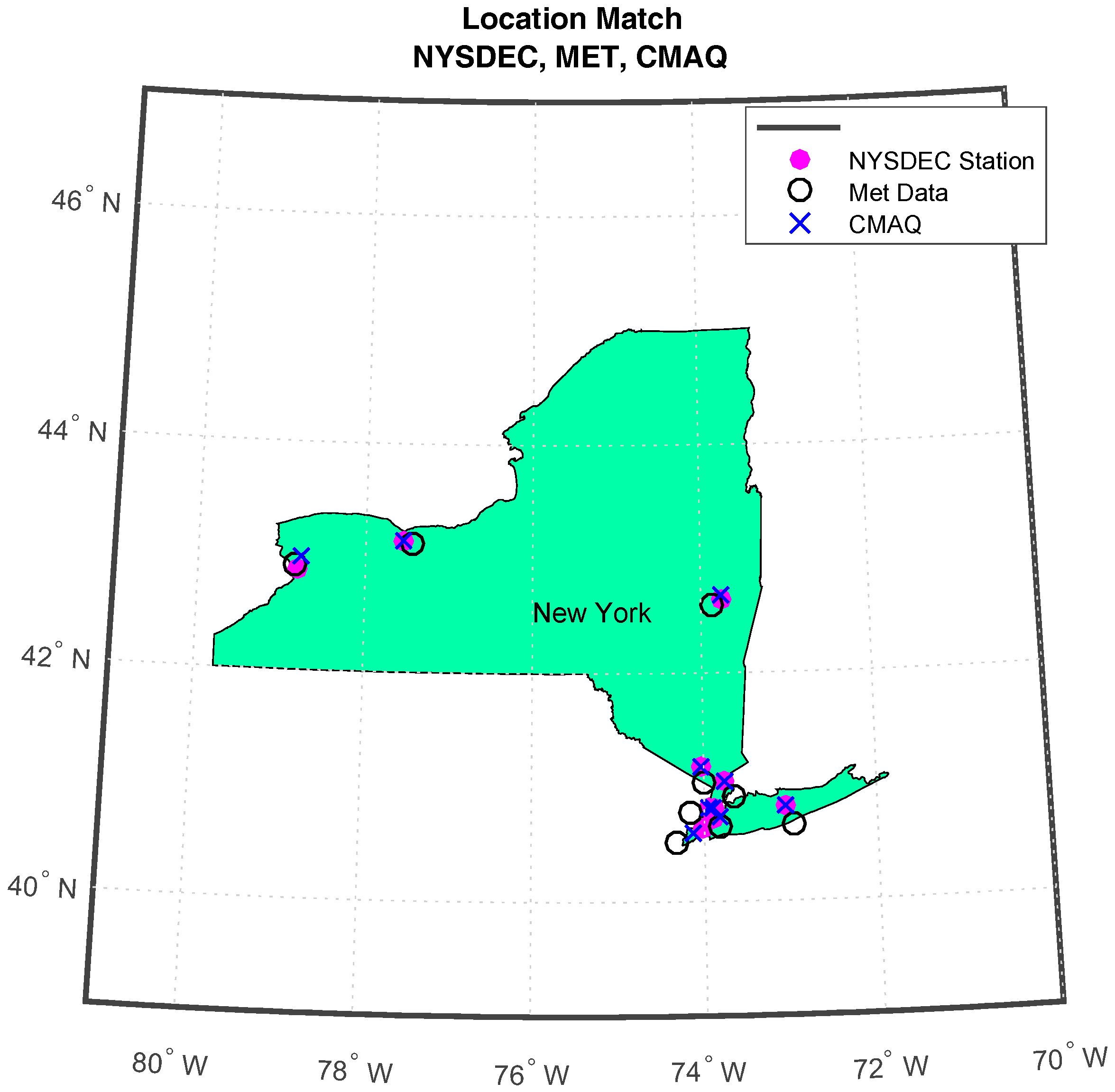
PM2.5 ground data is collected from the EPA’s AirNow, which collects NYSDEC monitoring station measurements in real time. The station data used for the forecast experiments in this article are from the New York State stations listed in Table A2, from 1 January 2011 until 31 December 2016. To assess the accuracy of CMAQ model forecasts, matching the model to the ground monitoring station is necessary. To do this, we use the ground NYSDEC stations that lay within the CMAQ grid cell only. Ground stations that are not found in a CMAQ grid cell were not used for comparison; therefore, no spatial interpolation was done on the model results while mapping the model or meteorological data to the AirNow ground stations. This matching method is widely used for comparing the CMAQ model to ground monitoring stations [6,7,14]. The locational data-points are depicted in Figure A1, the CMAQ grid cell information can be found in Table A1, and the NYSDEC station information can be found in Table A2.
2.2. Methods
Assessing Accuracy of CMAQ Forecasting Models
The forecasting skill of the different models were evaluated by computing the R2 and the root mean square (RMSE) values from a regression analysis comparing the model to the AirNow observations. High R2 values and low RMSE values indicated a good match between the prediction and the observations. Finally, to directly assess potential biases in the regression assessment, residual plots are provided to show significant concentration bias.
2.3. Results
2.3.1. Effects of Bias and Release Time
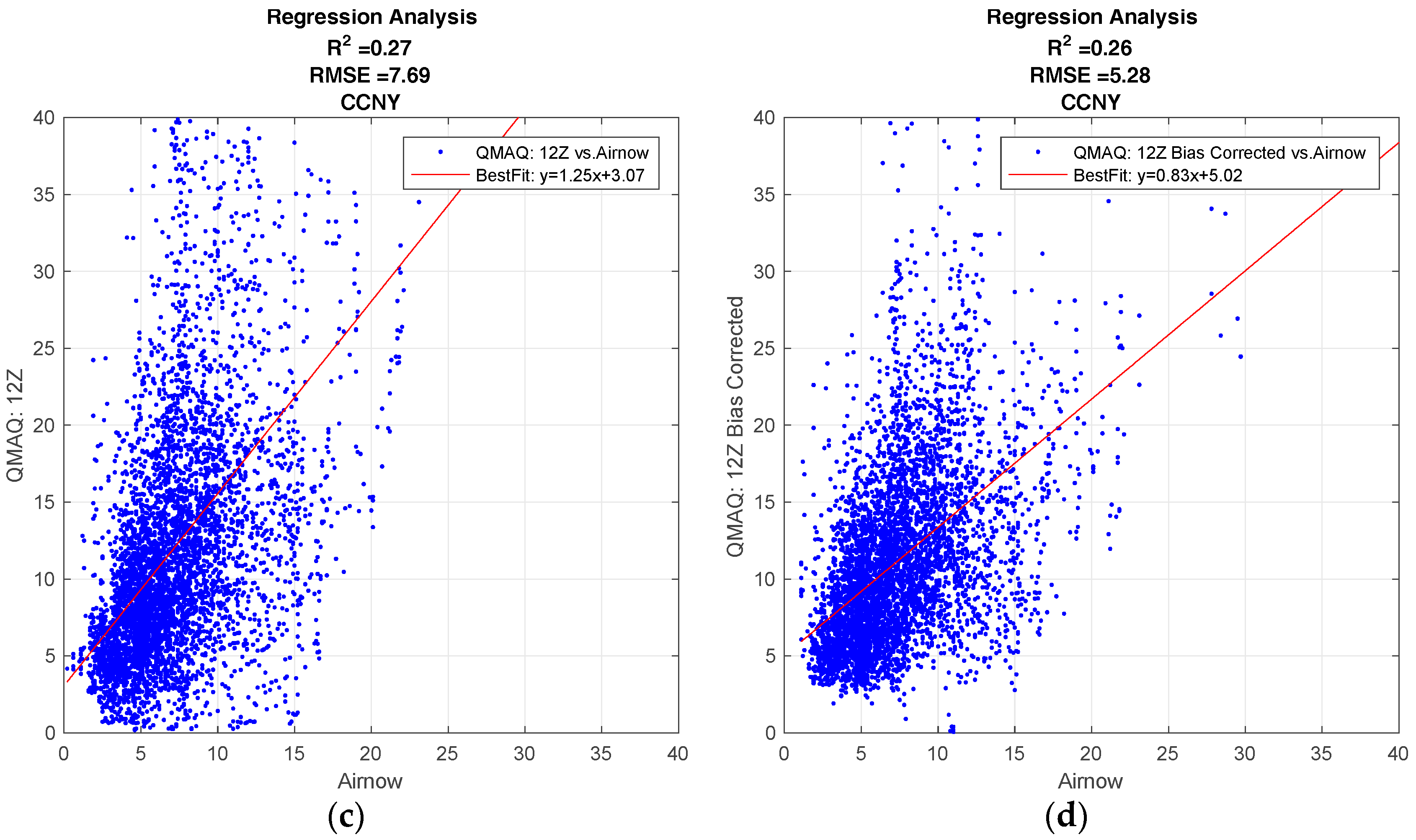
Figure 1 shows the regression plots for the hourly CMAQ model output compared to the ground station data for the City College of New York (CCNY Station) to illustrate the general behavior of the CMAQ model, and how the forecast is affected by different forecast release times, and by the bias corrections applied. The results of the R2 analysis for all ground stations can be found in the supplementary materials.
All forecasts from the CMAQ model over CCNY have a positive correlation to the ground data. The effect on the forecast for different release times, if any, is minimal.
As seen in Figure 1a,c, the standard model generally overestimates the ground. While the bias correction improves the over-prediction, the results are more dispersed. This can be verified from the fact that the bias correction decreases the root mean square error (RMSE), but it also decreases the R2 value for both release times.
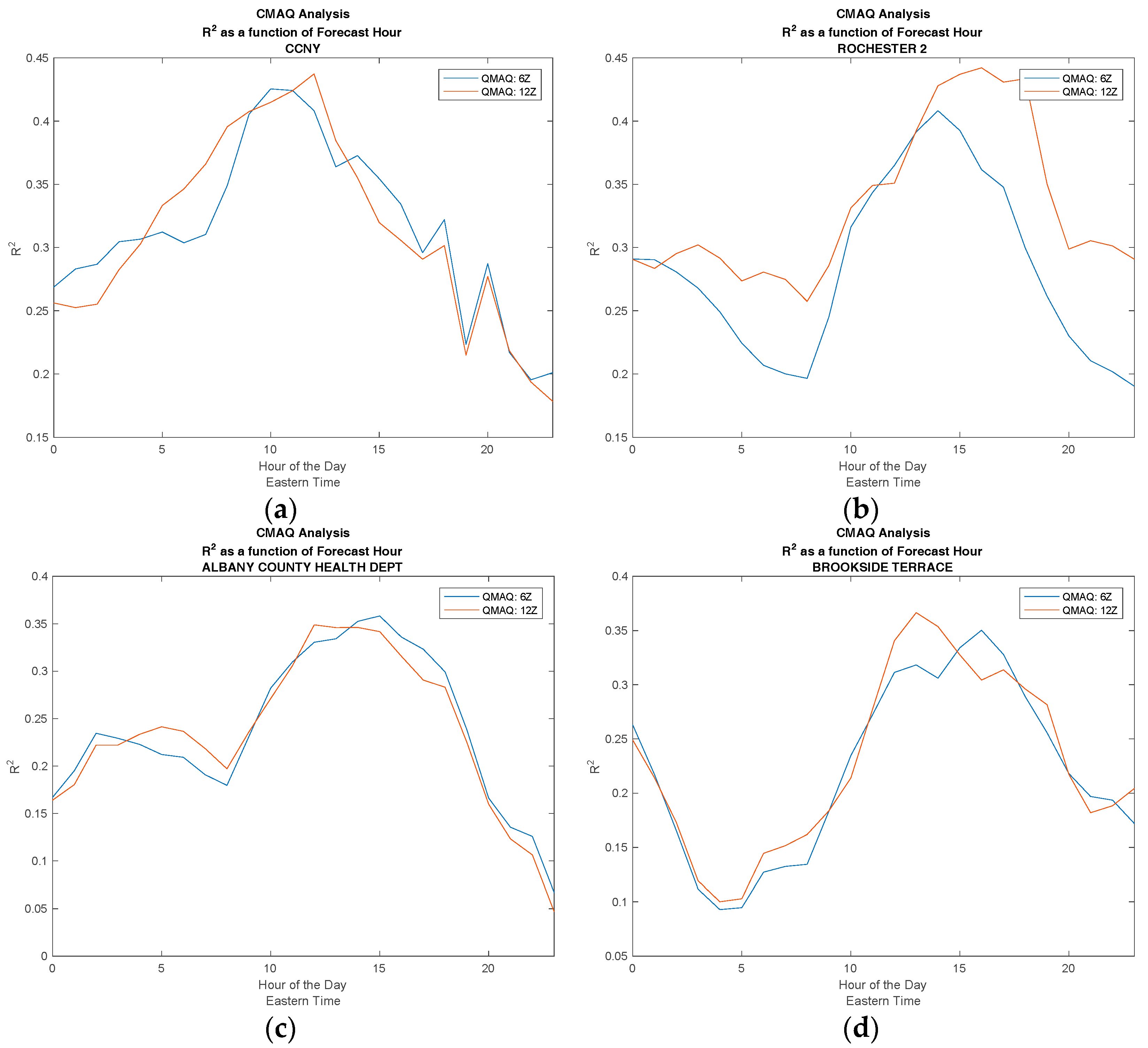
In Figure 1 we assess the overall skill for a 24-h CMAQ forecast. In Figure 2, we determine if the CMAQ model could be improved by simply moving the forecast release time to a later point in the day, thereby including the most up-to-date inputs in the model. To do this, we make a direct comparison between CMAQ forecasts with different release times. In Figure 2, the R2 value is computed for each hour of the day. The release time of 0600 UTC, with forecast hours of 22–45, is compared to the 1200 UTC release time, with forecast hours 16–39, to determine if the lower number of forecast hours yields more accurate predictions. It is clear from Figure 2 that the later release time does not lead to a significant improvement in the accuracy of the forecast, and this is true for both urban and non-urban test sites.
It can be seen from this analysis that the CMAQ model performs best for midday hours, which is reasonable, since this is the period when convective mixing is most dominant. As discussed in reference [9], PBL modeling is very complex during the predawn/post-sunset period and errors in the PBL height clearly are a significant concern for further model development.
2.3.2. Differences between Urban and Non-Urban Locations
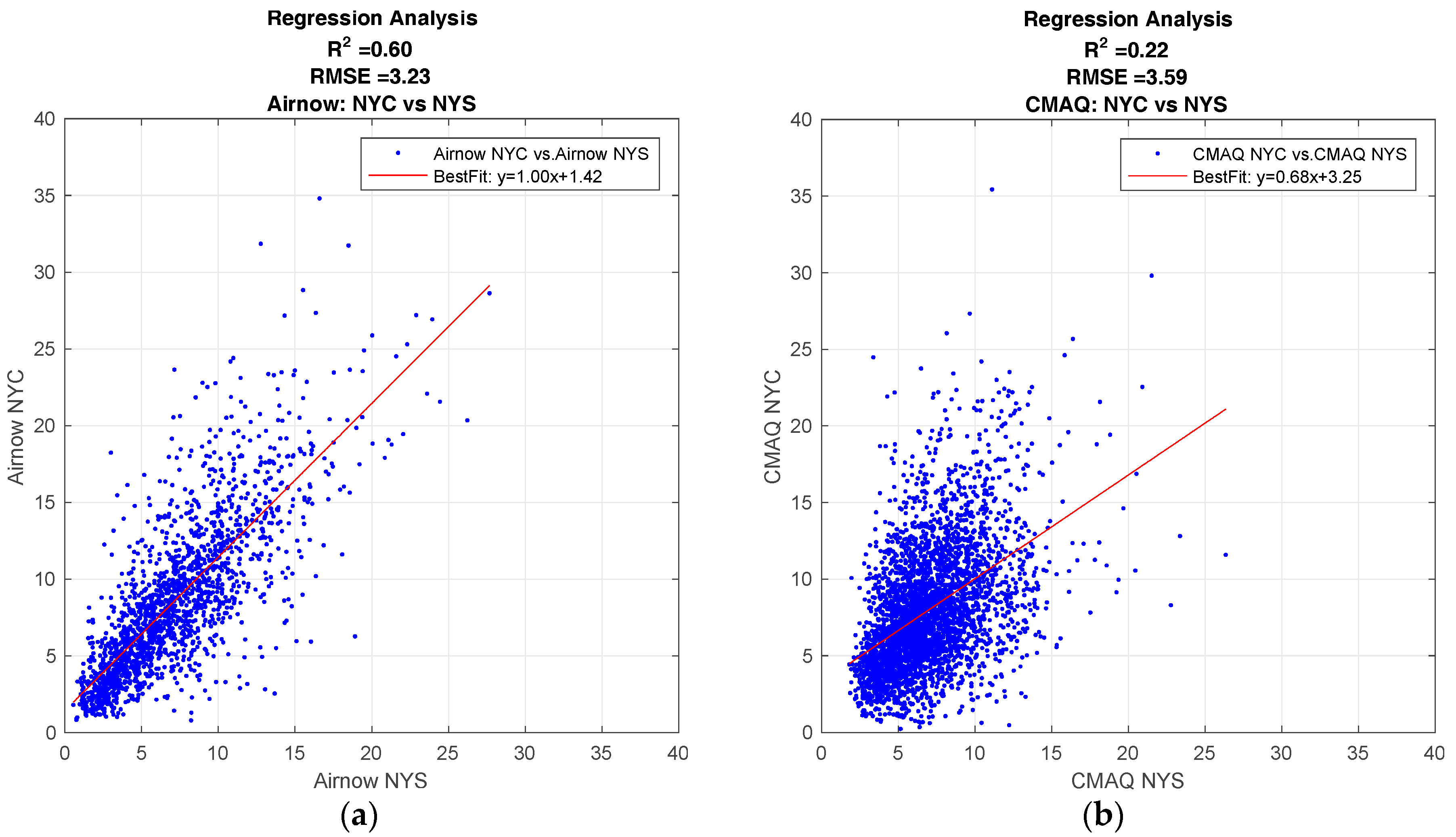
To get a better understanding of the spatial performance of the model, a multi-year time-series of daily averaged PM2.5 observations from ground monitoring is used to compare the relationship between PM2.5 values in New York City to the rest of New York State. Figure 3a is the regression analysis for this time period, and shows how the PM2.5 values for NYC are strongly correlated to non-NYC areas, R2 ~ 0.6. This indicates that while PM2.5 values in NYC are generally higher than the rest of the state, the PM2.5 level in NYC are still correlated to the levels in the rest of the state.
The same analysis comparing NYC to the rest of NYS was done with CMAQ forecast values as seen in Figure 3b. In this case, the correlation between NYC and NYS is not so strong, R2 ~ 0.2. From this analysis alone, we can only speculate the reason for a low correlation between CMAQ forecasts for NYC and the rest of NYS is due to strong spatial differences in the National Emission Inventory (NEI) entries. However, the strong correlation in ground observations between NYC and NYS shows that while urban source emission may be a significant cause for somewhat higher levels of PM2.5, there is still a strong correlation between NYC and NYS, and an accurate forecasting model must take this into account.
The limitations of CMAQ forecasting on a local pixel level indicate that other approaches should be explored. In particular, we explore the potential of data-driven models for localized forecasting in the next section.
3. Data Driven (Neural Network) Development
3.1. Datasets
3.1.1. Ground-Based Observations
PM2.5 data collected from NYSDEC ground-monitoring stations is used for inputs in the neural network. These are the same ground stations listed above, in Section 2.1.2.
3.1.2. Models
The meteorological data was collected from the National Centers for Environmental Prediction (NCEP) North American Regional Reanalysis (NARR). NARR has high-resolution reanalysis of the North American region, 0.3 degrees (32 km) at the lowest latitude, including assimilated precipitation. The NARR makes available 8-times-daily and monthly means respectively. The data collected for this paper is the 8-times-daily means for the duration 1 January 2011 until 31 December 2016. Figure A1 shows the proximity of the meteorological data and the CMAQ model outputs to the ground stations.
The NN network was created and tested using historical data. In this paper, meteorology “forecast” data refers to NARR data that was observed the day of the PM2.5 forecast. “Observed” or “measured” meteorology refers to NARR data that was observed before the forecast release time.
3.2. Methods
3.2.1. Development of the Neural Network
As stated above, the accurate prediction of PM2.5 values is crucial for air quality agencies, so that they could alert the public of the severity and duration of a high pollution event. Therefore, it is imperative that the forecast predictions are released to the public the day before the event. For this paper, we chose 5 p.m. as a target for the forecast release time. Therefore, we ensure that all the methods tested, utilize factors that are available to the state agency prior to 2100 UTC (5 p.m. EDT).
Input Selection Scenarios
The NN input includes the following NARR meteorological data: surface air temperature, surface pressure, planetary boundary layer height (PBLH), relative humidity, and horizontal wind (10 m). To account for the seasonal variations, the month is also used as an input in the neural network. The PM input variables for the NN are the PM2.5 measurements averaged over a three-hour frequency to match the meteorological dataset. The NN output is the next day PM2.5 values.
In order to optimize the performance of the neural network, preliminary tests were done to determine the optimum utilization of the meteorological input variables. These test were done to determine if the “forecast” or the “observed” meteorology, or a combination of the two, should be used as input variables.
The forecast time window is midnight-to-midnight EDT for the forecast day, while the time window with the observed data is midnight to 5 p.m. EDT the day the forecast is released.
For the PBLH, the forecast value is always used as the input. One NN design employed only the forecast meteorological values as inputs. The second design utilized a combination of the forecast and the observed data, by subtracting the eight observation datasets from the eight forecast datasets. This first NN architecture uses the meteorological values as predictors, while the second design uses metrological trends as predictors. We note that this comparison does not affect the number of inputs used, allowing for a direct comparison of information content.
In scenario 1, where only the MET forecasts are used, we use the following inputs, where i represents the indices for time windows for the observation day, and j represents the indices for time windows for the forecast day (from the NARR forecasts), the NN inputs design is:
| (Field measurements) | |||
| (NARR Forecasts) | |||
| (NARR Forecasts) |
In scenario 2, where the differential between the observation day and forecast day of the MET variables are used, the architecture for the NN inputs is:
| (Field measurements) | |||
| | | (NARR Forecasts) (NARR Observations) | |
| (NARR Forecasts) |
To show the robustness of the NN, the data used for training the neural networks came from 2011–2015 alone, while the network was tested with data from 2016. In both scenarios, the targets for the NN were taken to be the complete set of PM2.5 over all time windows of the forecast day:
| Targets: | (Field measurements) |
Neural Network Training Approach
In developing a NN PM2.5 forecast for all of New York State (NYS), we needed to take into account the very different emission sources, and to a lesser extent the meteorological conditions, between New York City (NYC) and the other sites in NYS. We found that the best solution is to design two different neural networks. The first is trained only over NYC sites, while the second is trained for the rest of NYS. It is important to note that we do not try to build a unique NN for every station, since this is not a useful approach for local agencies. PM and Meteorological data from 2011–2015, were used for training.
For NYC, since the stations are very close to each other, the NN was trained with spatial mean values of the ground PM monitors and NARR meteorological datasets. For NYS, all the PM and meteorological data from each site outside of NYC were used. Some site-specific information was implicitly included by using the surface pressure as inputs, which provides some indicator of surface elevation.
The neural network was developed using the MATLAB Neural Network Toolbox [15]. The Levenberg-Marquardt network was deployed using 10 hidden nodes. The break down for the NN input data is: 70% training, 15% validation, and 15% testing. Because the sample set of training, validation, and testing is divided randomly over the entire dataset, accuracy of the NN was determined by testing each network over 2016 data only, a time window that was not included in training. Once the NN function was created, the 2016 meteorological and PM data was passed through the network, and the outputs were stored with the date-time and station location as indices.
Neural Network Scenario Results
Figure 4a shows the performance of the NN using the forecast metrological data as inputs, while Figure 4b shows the performance of the NN using the difference between the forecast and the current days measurements. The NN utilizing the difference configuration is clearly better, with a higher R2 value, 0.44 compared to 0.36, and a lower root-mean-square value, 3.09 compared to 4.59. In addition, there are substantially less anomalous high PM2.5 forecasts. Since this improvement was seen in all test cases, we only used scenario 2, (differential meteorology) NN configuration. From these results, we see that meteorological trends are better indicators of PM2.5 than meteorology alone. This appears to us to be a reasonable result since the meteorology trend better isolates particular mesoscale conditions, which is known to be a significant factor in boundary layer dynamics.
3.3. Results
3.3.1. Neural Network and CMAQ Comparison
The R2 value for CMAQ and the NN, both compared to AirNow observations, is computed for each forecast model and for each location. As a representative example of the overall performance, the R2 value for NYC, represented by CCNY, is compared to NYS, represented by Brookside Terrace, a non-NYC, non-urban station, and these results are displayed in Figure 5. The individual results for each location can be found in the supplementary materials.
From Figure 5 above, it can be seen that the most accurate forecast model is the neural network for both NYS and NYC over any of the CMAQ forecasts studied. Regarding CMAQ, we note better performance for NYC than for non-urban areas. This is in contrast to the neural network, where there is very little variation in the results for locations that are urban versus non-urban, indicating that locational inputs in the model, such as the surface pressure, improves forecasting skill.
In addition, for all cases, it can be seen that taking the time average improves the CMAQ results. Furthermore, the spatial averaging over NYS (with 1-h time sampling) shows more improvement in most NYC cases and some non-NYC cases as well. These results indicate the possibility that the best use for CMAQ forecasting is on a regional level. This is supported from the 12 km grid cell resolution for CMAQ, a cell size typical for regional analysis.
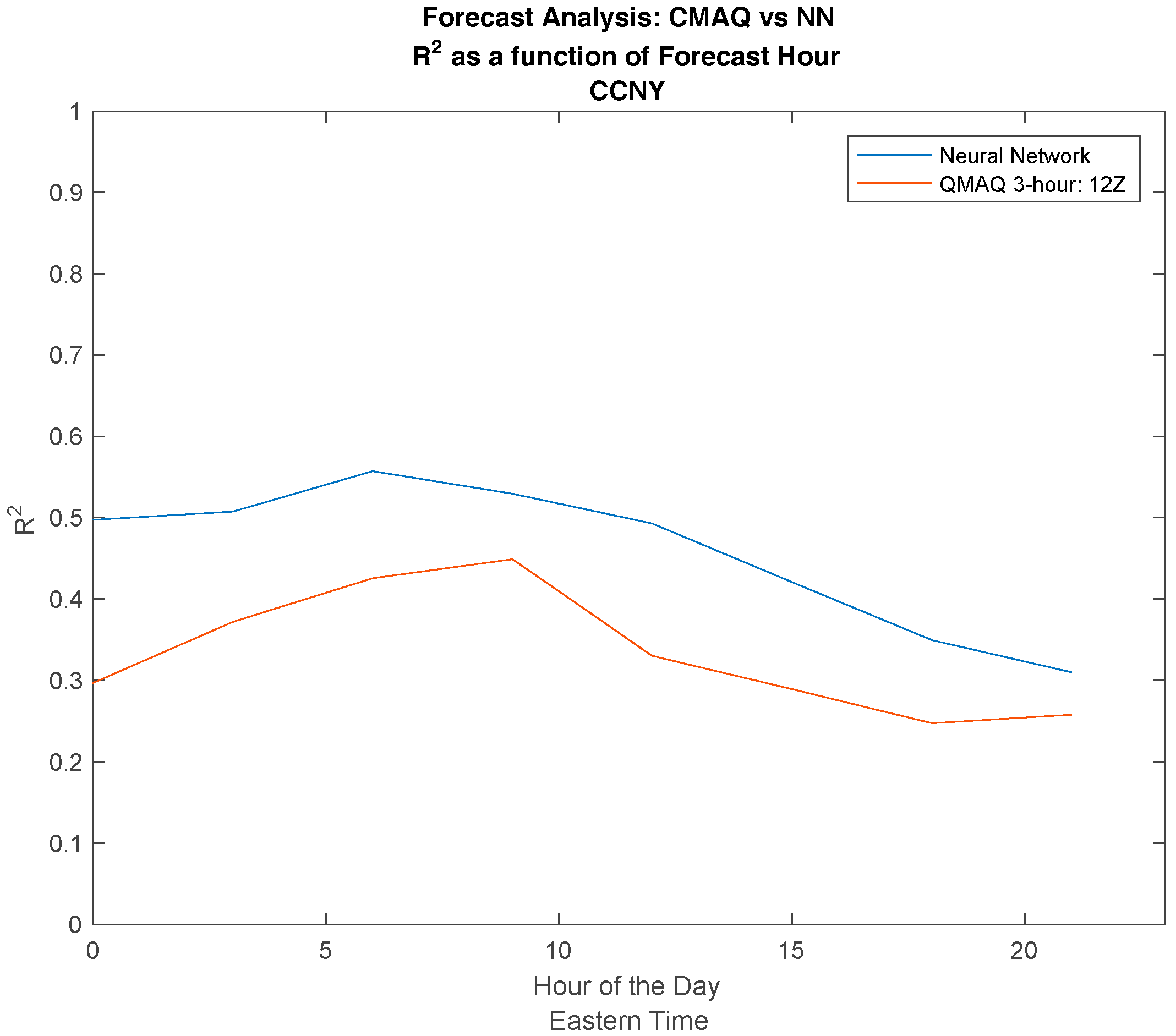
We note again that the different release times for CMAQ has almost no effect on the forecast accuracy. In Figure 6, we compared the diurnal performance of the NN to the CMAQ model. The most apparent result is the dramatic improvement of the NN during the night and morning hours, where the CMAQ model has the most difficulty. This is clearly due to the machine learning approach where the time differences, the inputs, and forecast periods have a dramatic effect on output performance.
This also explains the general downward trend, where performance tails off in the late afternoon and becomes closer to the CMAQ performance. This can be expected, because larger time delays should lead to more dispersion between the outputs and input PM levels.
Figure 7 below shows the residual results for CMAQ in comparison to the neural network. For CMAQ, as noted above, there seems to exist a non-random bias pattern, where CMAQ generally over predicts for low and high PM values, and under predicts for medium values. This pattern seems to indicate that the CMAQ model may not capture all of the underlying variability factors. On the other hand, for the neural network, the behavior of the residuals is clearly stochastic in nature.
We find that an optimized NN approach generally results in a more accurate prediction of future pollution levels, as compared to CMAQ, for a single grid cell (resolution 12 km).
3.3.2. Heavy Pollution Transport Events
Because the neural network is data-driven, the network performs better when the most up-to-date inputs are used. This explains the degradation of performance with time, as seen in Figure 6. In the current design of the neural network, we only used five PM2.5 inputs, instead of maximum possible in a 24-h period, eight. In the training of the NN, there were very few extreme event cases, PM2.5 > 25 μg/m3. The lack of suitable training statistics for these events causes the NN approach to have difficultly in adjusting to the sharp contrast with the onset of the event.
Therefore, a second neural network was trained with the same design as the neural network illustrated above; however, this neural network produces a 24-h forecast at 5 p.m. for the time period, 5 p.m.–5 p.m. (instead of a next day 24-h midnight-to-midnight forecast). This neural network uses all eight PM measurements, because there is no lag time between the release time and the first forecast hour. This neural network, referred to as NN Continuous, was not used in the statistical analysis for the different forecast models (because the 24-h forecast period is different than the forecast analysis above), but is being explored in the extreme event cases. The reason for developing this continuous neural network is to determine if the continuous nature of the network produces better results in extreme pollution events.
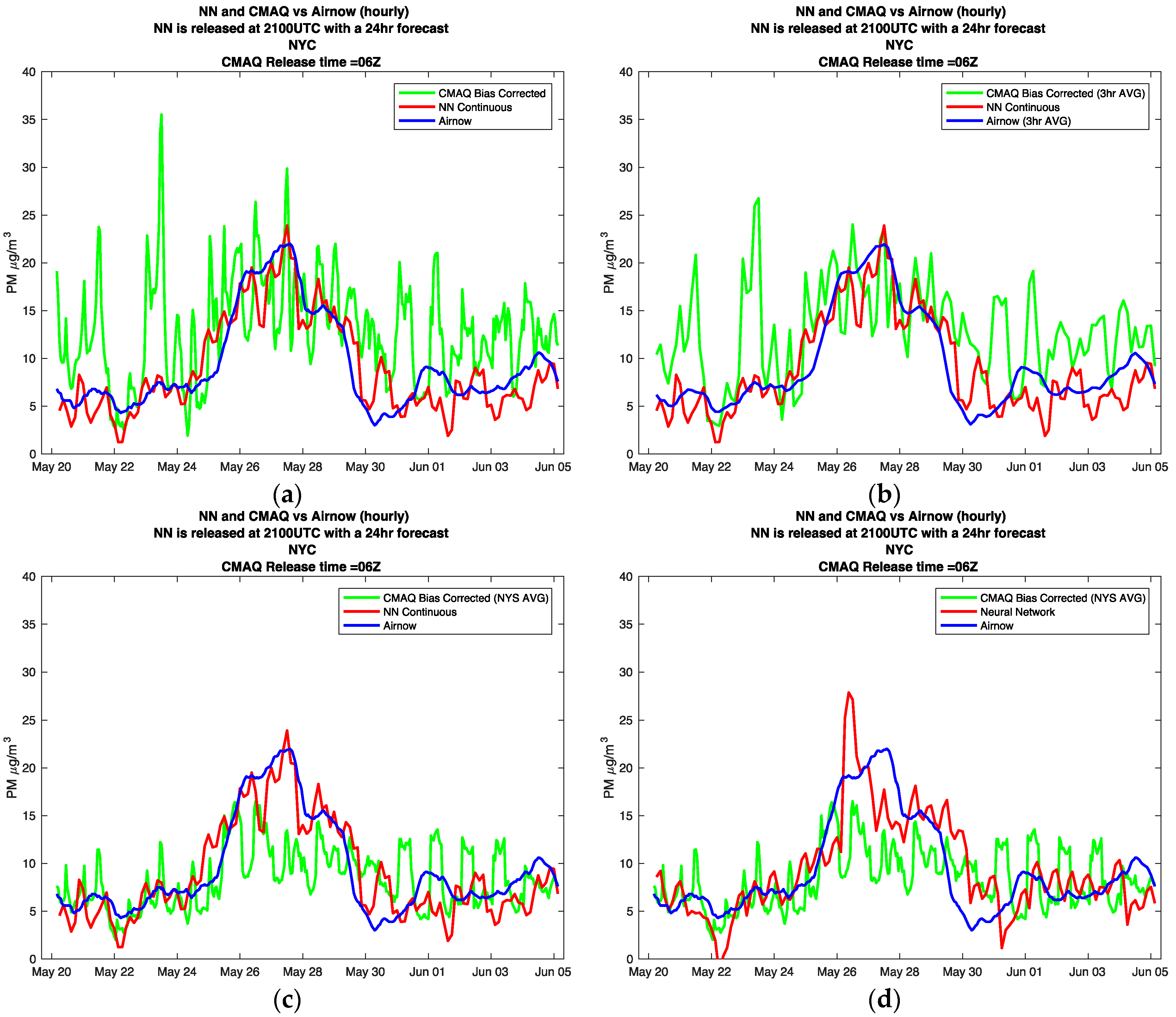
To explore the behavior of the different models under high pollution transport conditions, the forecasts coinciding with the wildfires of Fort McMurray in Alberta, Canada were analyzed. The wildfire started on 1 May 2016, and was declared under control on 5 July 2016. Although the wildfire lasted for over two months, evidence of increased PM2.5 surface levels in NYC resulting from the wildfire were detected on 9 May, and on 25 May. On these dates, instances of aloft plume intrusions and the mixing down into the planetary-boundary layer were observed by a ceilometer and a Raman-Mie Lidar [16]. In Figure 8, we plot the CMAQ and NN model forecasts, focusing on the transport intrusions into NYC on 25 May.
The first thing to notice in Figure 8a, is the oscillations in the CMAQ model, and to notice how these oscillations smooth out in Figure 8b,c, where the three-hour time average and the New York State spatial average are tested respectively. It is logical that for heavy transport cases, domain averaging helps decrease oscillations; however, we still see significant underestimation of the event.
This is the first case where we analyze the behavior of the continuous neural network. Looking at Figure 8c,d, it is clear that the continuous neural network is able to respond to the trend of the high pollution event faster, and more accurately, then the standard neural network.
4. Conclusions
In this paper, we first made a baseline assessment of the V4.6 CMAQ forecasts, and found significant dispersion as well as a tendency for the model to overestimate the ground truth field measurements. Even in the bias corrected case, the residuals error in the model was found to have significant bias patterns, indicating that there are predictors not included in the model that could significantly improve the results.
These results motivated the development of data driven approaches such as a NN. In developing a data driven NN next day forecast model, we found a general improvement of performance when using prior PM2.5 inputs together with the difference between present and next day meteorological parameter forecasts. This “differential NN” approach performed significantly better than if we used only the future forecast variables, indicating that meteorological pattern trends are important indicators.
Using this NN architecture, we then made extensive regression based comparisons between CMAQ next day forecast models and regionally trained NN next day forecasts for the NYS and NYC regions. In general, we found that the NN results are a significant improvement over the CMAQ forecasts in all cases. These comparisons were made to be consistent with state agencies where forecasts should be available by 5 p.m. In addition, we also made a diurnal comparison, which illustrated that; the NN approach had superior forecasting skills during the early part of the day but degraded smoothly as the forecast time increased. By mid-day, the differences between the two approaches was much closer.
To improve the CMAQ forecasts, we found limited improvement when spatial averaging is extended beyond the single pixel 12 km resolution to all of New York State. Even in this case, the NN results were generally more accurate.
Finally, we focused on forecast performance for transported high pollution events such as Canadian wildfires. In these cases, we found that the CMAQ forecasts had large temporal fluctuations, which could hide most of the event. In this case, significant improvement was obtained when using state averaged bias corrected outputs; however, in general, the smoothed results underestimate the local PM2.5 measurements.
In this application, we found the neural network approach provides a reasonably smooth forecast, although the transition from a clean state to a polluted state is very poor. Nevertheless, the standard NN performed better than CMAQ in this scenario. Further improved results for the NN were obtained in the transition period when the forecast time of the NN was reduced (NN continuous), making the transition from training to testing continuous.
Future Work
While the continuous NN does adjust quickly to the sharp contrast in transport events, this design limits the scope of the forecast period. Clearly, local data alone is not ideal for this application. Non-local data that can identify high pollution events and assesses their potential mixing with our region is needed. As a preliminary analysis, we explored the use of a combination of HYSPLIT Air Parcel Trajectories with GOES satellite Aerosol Optical Depth (AOD) retrievals to improve the NN. In particular, we analyzed the use of these tools to quantify the relative AOD levels for all air parcels that reach our target area. We found that by properly counting the trajectories weighted by the AOD, a good correlation was seen between the relative AOD and the PM2.5 levels. Therefore, we believe that using the relative AOD metric as an additional input factor can make improvements in the NN approach. When GOES-R AOD retrievals, with high data latency and multispectral inversion capabilities [17,18], become available, we plan to incorporate these AOD metrics as predictors in the NN.
Supplementary Materials
The following are available online at www.mdpi.com/2073-4433/8/9/161/s1, Figure S1: Regression Analysis.
Acknowledgments
The authors gratefully acknowledge the NOAA Air Resources Laboratory (ARL) for the provision of the HYSPLIT transport and dispersion model used in this publication. We further gratefully acknowledge Jeff McQueen for providing the V4.6 CMAQ forecasts. Finally, S. Lightstone would like to acknowledge partial support of this project through a NYSERDA EMEP Fellowship award.
Author Contributions
Samuel Lightstone was responsible for the NN experiments and the CMAQ assessment; Lightstone also wrote the paper. Barry Gross was responsible for design of the different experiments as well as conceiving the use of the GOES AOD and HYSPLIT trajectories to estimate transported AOD as a predictor of PM2.5. Fred Moshary provided significant critical assessment and suggestions of all results.
Conflicts of Interest
The authors declare no conflict of interest.
Appendix A. Datasets

Table A1.
CMAQ Grid Cell Information.
| Name | Abbreviation | Latitude | Longitude | Land Type |
|---|---|---|---|---|
| Amherst | AMHT | 42.99 | −78.77 | Suburban |
| CCNY | CCNY | 40.82 | −73.95 | Urban |
| Holtsville | HOLT | 40.83 | −73.06 | Suburban |
| IS 52 | IS52 | 40.82 | −73.90 | Suburban |
| Loudonville | LOUD | 42.68 | −73.76 | Urban |
| Queens College 2 | QC2 | 40.74 | −73.82 | Suburban |
| Rochester Pri 2 | RCH2 | 43.15 | −77.55 | Urban |
| Rockland County | RCKL | 41.18 | −74.03 | Rural |
| S. Wagner HS | WGHS | 40.60 | −74.13 | Urban |
| White Plains | WHPL | 41.05 | −73.76 | Suburban |
Table A2.
NYSDEC Station Information.
| NYSDEC ID | Station Name | Latitude | Longitude | Land Type |
|---|---|---|---|---|
| 360010005 | Albany County Health Dept | 42.6423 | −73.7546 | Urban |
| 360050112 | IS 74 | 40.8155 | −73.8855 | Suburban |
| 360291014 | Brookside Terrace | 42.9211 | −78.7653 | Suburban |
| 360551007 | Rochester 2 | 43.1462 | −77.5482 | Urban |
| 360610135 | CCNY | 40.8198 | −73.9483 | Urban |
| 360810120 | Maspeth Library | 40.7270 | −73.8931 | Suburban |
| 360850055 | Freshkills West | 40.5802 | −74.1983 | Suburban |
| 360870005 | Rockland County | 41.1821 | −74.0282 | Rural |
| 361030009 | Holtsville | 40.8280 | −73.0575 | Suburban |
| 361192004 | White Plains | 41.0519 | −73.7637 | Suburban |
Figure A1.
This map shows the proximity of the ground NYSDEC stations to the NARR meteorological data, and the CMAQ forecast data.
Figure A1.
This map shows the proximity of the ground NYSDEC stations to the NARR meteorological data, and the CMAQ forecast data.

References
- Pope, C.A., III; Dockery, D.W. Health effects of fine particulate air pollution: Lines that connect. J. Air Waste Manag. Assoc. 2006, 56, 709–742. [Google Scholar] [CrossRef] [PubMed]
- Pope, C.A., III; Burnett, R.T.; Thun, M.J.; Calle, E.E.; Krewski, D.; Ito, K.; Thurston, G.D. Lung cancer, cardiopulmonary mortality, and long-term exposure to fine particulate air pollution. JAMA 2002, 287, 1132–1141. [Google Scholar] [CrossRef] [PubMed]
- Weber, S.A.; Insaf, T.Z.; Hall, E.S.; Talbot, T.O.; Huff, A.K. Assessing the impact of fine particulate matter (PM2.5) on respiratory-cardiovascular chronic diseases in the New York City Metropolitan area using Hierarchical Bayesian Model estimates. Environ. Res. 2016, 151, 399–409. [Google Scholar] [CrossRef] [PubMed]
- Rattigan, O.V.; Felton, H.D.; Bae, M.; Schwab, J.J.; Demerjian, K.L. Multi-year hourly PM2.5 carbon measurements in New York: Diurnal, day of week and seasonal patterns. Atmos. Environ. 2010, 44, 2043–2053. [Google Scholar] [CrossRef]
- Byun, D.; Schere, K.L. Review of the governing equations, computational algorithms, and other components of the Models-3 Community Multiscale Air Quality (CMAQ) modeling system. Appl. Mech. Rev. 2006, 59, 51–77. [Google Scholar] [CrossRef]
- McKeen, S.; Chung, S.H.; Wilczak, J.; Grell, G.; Djalalova, I.; Peckham, S.; Gong, W.; Bouchet, V.; Moffet, R.; Tang, Y.; et al. Evaluation of several PM2.5 forecast models using data collected during the ICARTT/NEAQS 2004 field study. J. Geophys. Res. Atmos. 2007, 112. [Google Scholar] [CrossRef]
- Yu, S.; Mathur, R.; Schere, K.; Kang, D.; Pleim, J.; Young, J.; Tong, D.; Pouliot, G.; McKeen, S.A.; Rao, S.T. Evaluation of real-time PM2.5 forecasts and process analysis for PM2.5 formation over the eastern United States using the Eta-CMAQ forecast model during the 2004 ICARTT study. J. Geophys. Res. Atmos. 2008, 113. [Google Scholar] [CrossRef]
- Huang, J.; McQueen, J.; Wilczak, J.; Djalalova, I.; Stajner, I.; Shafran, P.; Allured, D.; Lee, P.; Pan, L.; Tong, D.; et al. Improving NOAA NAQFC PM2.5 Predictions with a Bias Correction Approach. Weather Forecast. 2017, 32, 407–421. [Google Scholar] [CrossRef]
- Doraiswamy, P.; Hogrefe, C.; Hao, W.; Civerolo, K.; Ku, J.Y.; Sistla, G. A retrospective comparison of model-based forecasted PM2.5 concentrations with measurements. J. Air Waste Manag. Assoc. 2010, 60, 1293–1308. [Google Scholar] [CrossRef] [PubMed]
- Gan, C.-M.; Wu, Y.; Madhavan, B.L.; Gross, B.; Moshary, F. Application of active optical sensors to probe the vertical structure of the urban boundary layer and assess anomalies in air quality model PM2.5 forecasts. Atmos. Environ. 2011, 45, 6613–6621. [Google Scholar] [CrossRef]
- Files in /mmb/aq/sv/grib. Available online: http://www.emc.ncep.noaa.gov/mmb/aq/sv/grib/ (accessed on 1 December 2016).
- NCEP Operational Air Quality Forecast Change Log. Available online: http://www.emc.ncep.noaa.gov/mmb/aq/AQChangelog.html (accessed on 1 May 2017).
- Lee, P.; McQueen, J.; Stajner, I.; Huang, J.; Pan, L.; Tong, D.; Kim, H.; Tang, Y.; Kondragunta, S.; Ruminski, M.; et al. NAQFC developmental forecast guidance for fine particulate matter (PM2.5). Weather Forecast. 2017, 32, 343–360. [Google Scholar] [CrossRef]
- McKeen, S.; Grell, G.; Peckham, S.; Wilczak, J.; Djalalova, I.; Hsie, E.; Frost, G.; Peischl, J.; Schwarz, J.; Spackman, R.; et al. An evaluation of real-time air quality forecasts and their urban emissions over eastern Texas during the summer of 2006 Second Texas Air Quality Study field study. J. Geophys. Res. Atmos. 2009, 114. [Google Scholar] [CrossRef]
- Demuth, H.; Beale, M. MATLAB and Neural Network Toolbox Release 2016a; The MathWorks, Inc.: Natick, MA, USA, 1998. [Google Scholar]
- Wu, Y.; Pena, W.; Diaz, A.; Gross, B.; Moshary, F. Wildfire Smoke Transport and Impact on Air Quality Observed by a Multi-Wavelength Elastic-Raman Lidar and Ceilometer in New York City. In Proceedings of the 28th International Laser Radar Conference, Bucharest, Romania, 25–30 June 2017. [Google Scholar]
- Anderson, W.; Krimchansky, A.; Birmingham, M.; Lombardi, M. The Geostationary Operational Satellite R Series SpaceWire Based Data System. In Proceedings of the 2016 International SpaceWire Conference (SpaceWire), Yokohama, Japan, 25–27 October 2016. [Google Scholar]
- Lebair, W.; Rollins, C.; Kline, J.; Todirita, M.; Kronenwetter, J. Post launch calibration and testing of the Advanced Baseline Imager on the GOES-R satellite. In Proceedings of the SPIE Asia-Pacific Remote Sensing, New Delhi, India, 3–7 April 2016. [Google Scholar]
Figure 1.
Community Multi-Scale Air Quality (CMAQ) regression analysis. (a) Standard, 06Z release time; (b) Bias Corrected, 06Z release time; (c) Standard, 12Z release time; (d) Bias Corrected, 12Z release time.
Figure 1.
Community Multi-Scale Air Quality (CMAQ) regression analysis. (a) Standard, 06Z release time; (b) Bias Corrected, 06Z release time; (c) Standard, 12Z release time; (d) Bias Corrected, 12Z release time.
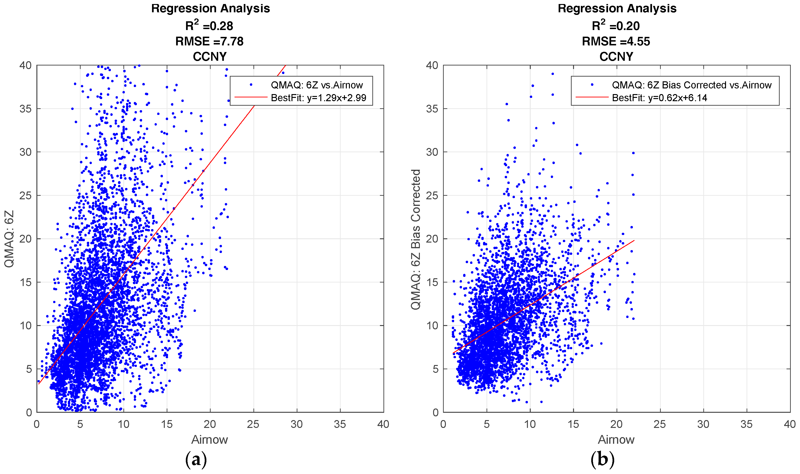

Figure 2.
Comparing the effect of different release times for CMAQ by plotting the R2 value as a function of time of day. (a) City College of New York (CCNY); (b) Rochester; (c) Albany; (d) Brookside Terrace.
Figure 2.
Comparing the effect of different release times for CMAQ by plotting the R2 value as a function of time of day. (a) City College of New York (CCNY); (b) Rochester; (c) Albany; (d) Brookside Terrace.

Figure 3.
Regression analysis comparing PM2.5 levels between NYC and the rest of NYS (non-NYC sites). (a) Multi-year day-averaged PM2.5 analysis from NYSDEC ground observations; (b) CMAQ model comparison between NYC and NYS.
Figure 3.
Regression analysis comparing PM2.5 levels between NYC and the rest of NYS (non-NYC sites). (a) Multi-year day-averaged PM2.5 analysis from NYSDEC ground observations; (b) CMAQ model comparison between NYC and NYS.

Figure 4.
Results from the regression analysis to maximize Neural Network performance for the different scenarios. (a) NN designed with the forecast meteorological data (Scenario 1); (b) NN designed by taking the difference between the forecast and the current days measurements (Scenario 2).
Figure 4.
Results from the regression analysis to maximize Neural Network performance for the different scenarios. (a) NN designed with the forecast meteorological data (Scenario 1); (b) NN designed by taking the difference between the forecast and the current days measurements (Scenario 2).
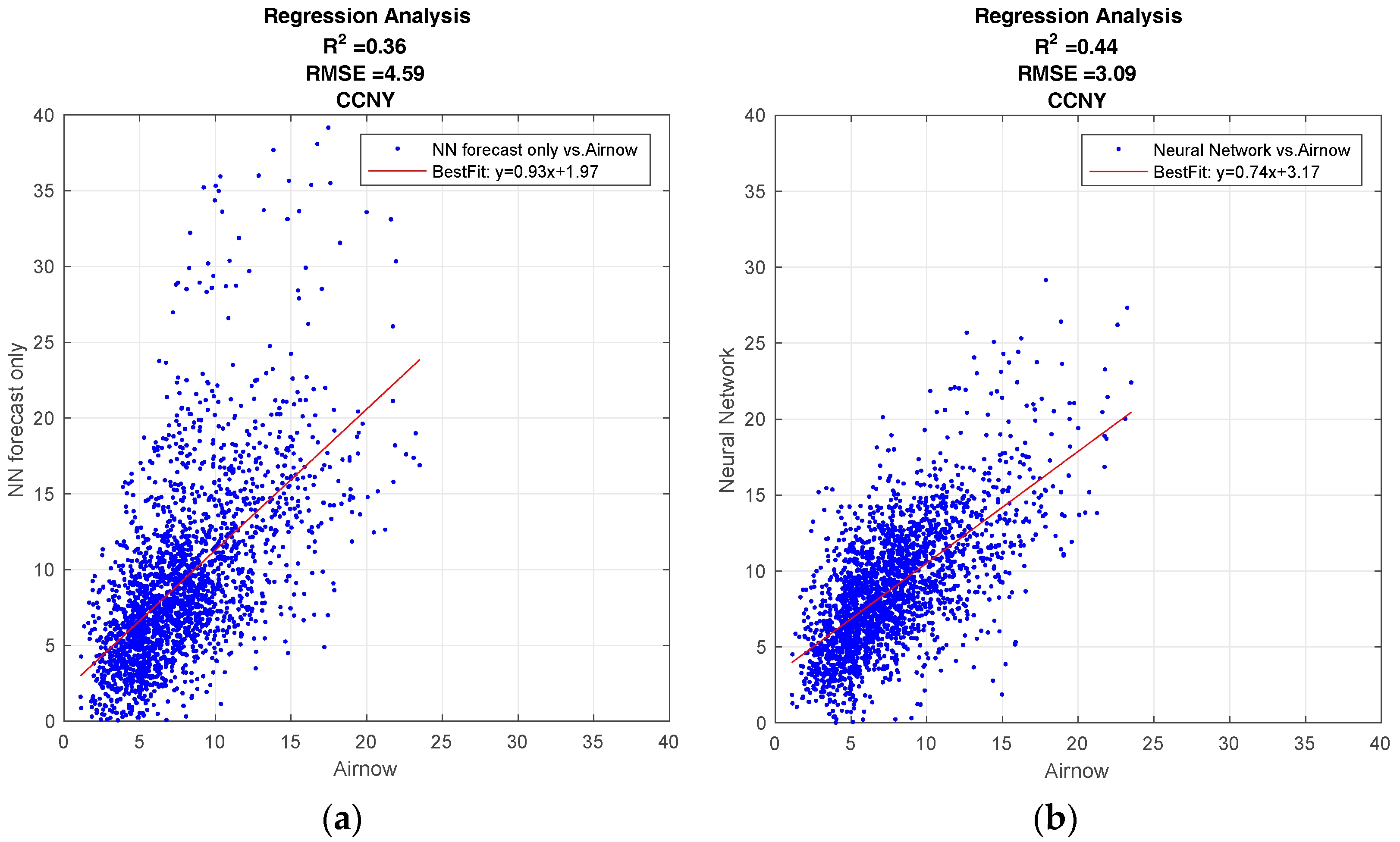
Figure 5.
Regression analysis is computed for the comparison between AirNow observations and the various prediction models, for the complete CMAQ database time period (February 2016, through October 2016). The R2 value for each model is plotted in the figure above to compare CMAQ to the NN. The CMAQ model includes the different release times as well as bias compensated vs. uncompensated runs. In addition, different time and spatial averaging of CMAQ is considered at each location. (a) Brookside Terrace, representative of non-NYC; (b) CCNY, representative of NYC.
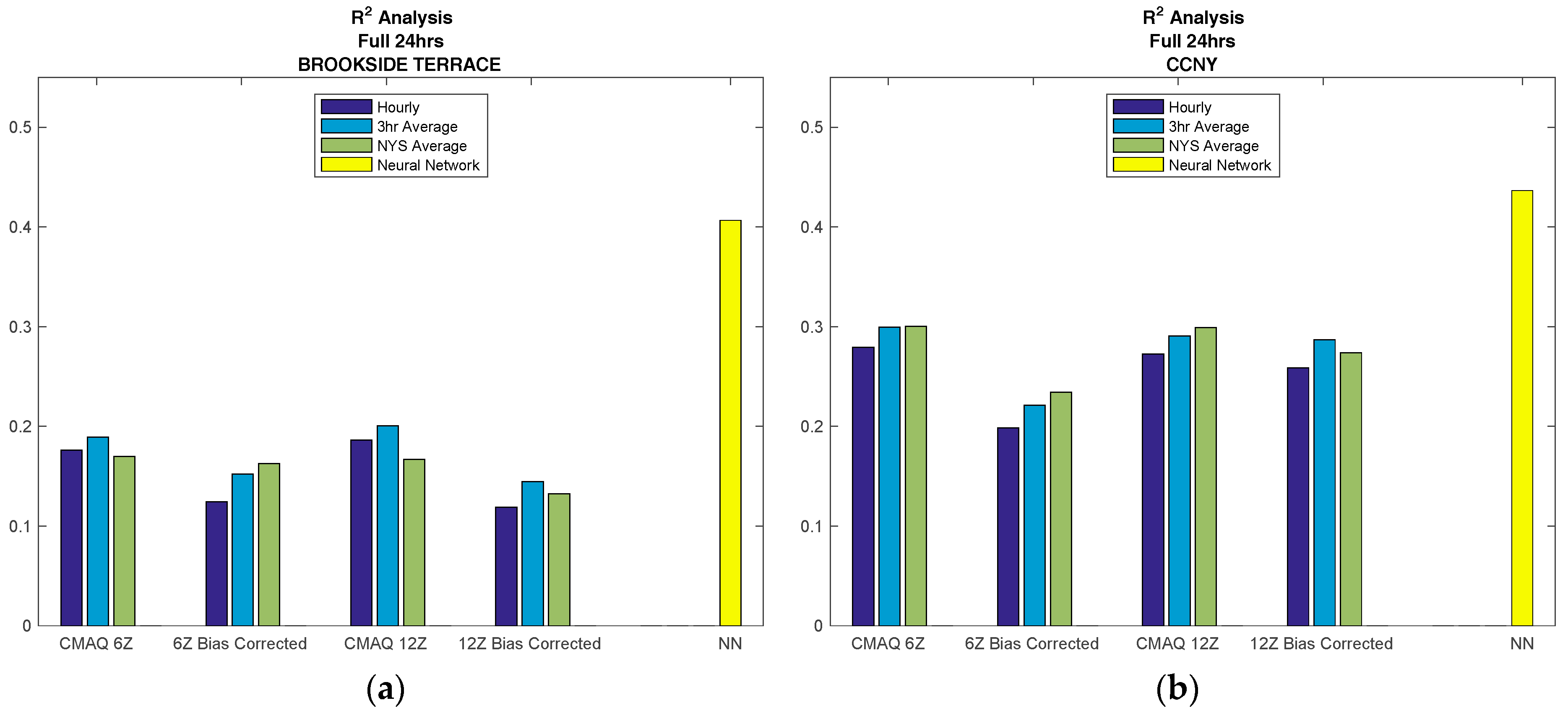
Figure 6.
Comparing the effect of different release times for the NN in comparison to CMAQ by plotting the R2 value as a function of time of day.
Figure 6.
Comparing the effect of different release times for the NN in comparison to CMAQ by plotting the R2 value as a function of time of day.

Figure 7.
Residual analysis. The standard deviation of PM2.5 from the AirNow ground monitoring sites was calculated to be 4 μg/m3, therefore, +/−4 μg/m3 was used for the error bounds (a) CMAQ; (b) Neural Network.
Figure 7.
Residual analysis. The standard deviation of PM2.5 from the AirNow ground monitoring sites was calculated to be 4 μg/m3, therefore, +/−4 μg/m3 was used for the error bounds (a) CMAQ; (b) Neural Network.
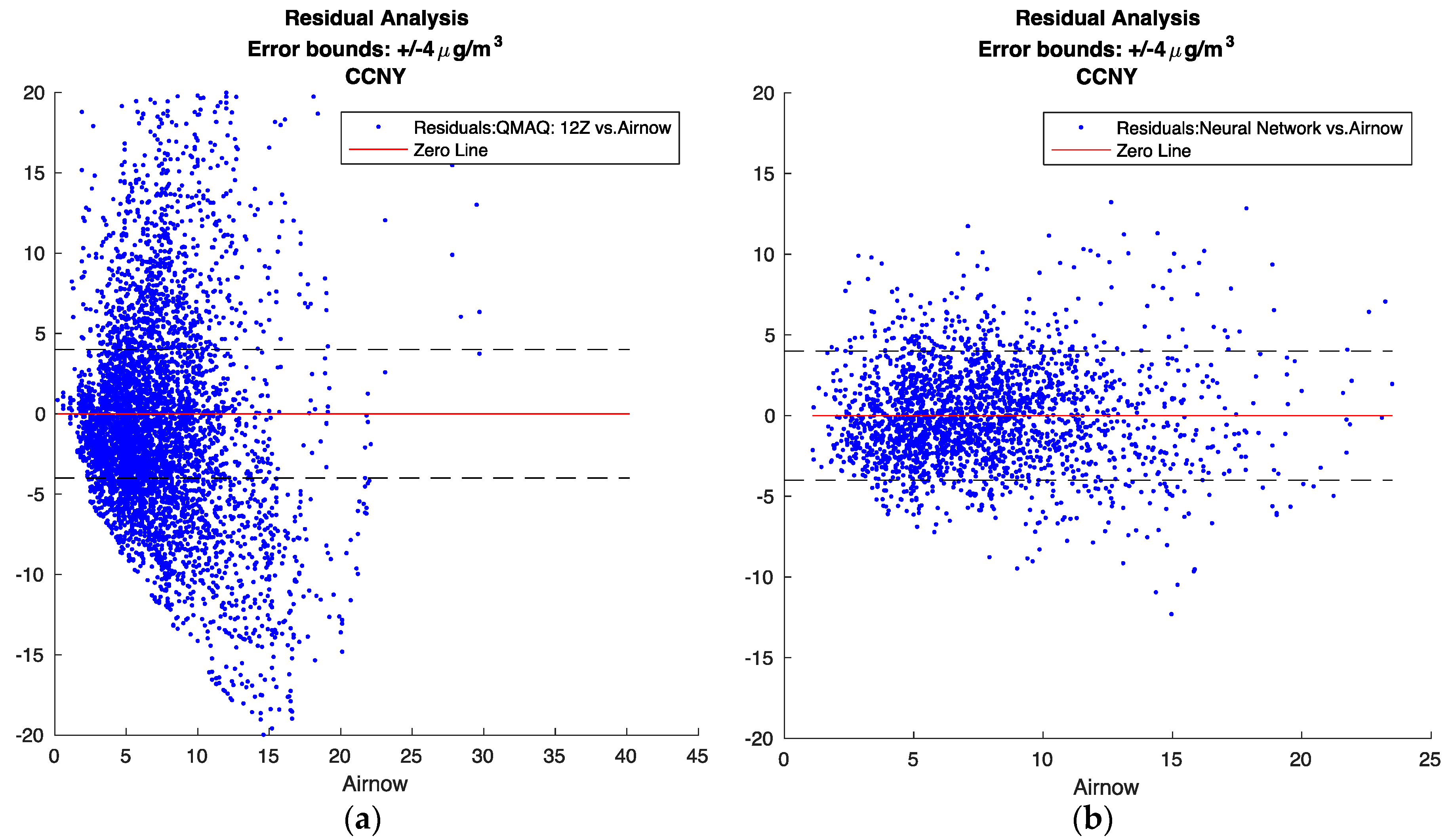
Figure 8.
NYC surface PM2.5 levels affected from the wildfires of Alberta Canada 2016. The plots focus on the aloft plumes mixing down into the PBL on May 25. The plots show different models vs. AirNow observation (a) CMAQ Biased hourly, NN continuous; (b) CMAQ Biased 3-h average, NN continuous; (c) CMAQ Biased state average, NN continuous; (d) CMAQ Biased state average, standard Neural Network.

© 2017 by the authors. Licensee MDPI, Basel, Switzerland. This article is an open access article distributed under the terms and conditions of the Creative Commons Attribution (CC BY) license (http://creativecommons.org/licenses/by/4.0/).
Share and Cite
MDPI and ACS Style
Lightstone, S.D.; Moshary, F.; Gross, B. Comparing CMAQ Forecasts with a Neural Network Forecast Model for PM2.5 in New York. Atmosphere 2017, 8, 161. https://doi.org/10.3390/atmos8090161
AMA Style
Lightstone SD, Moshary F, Gross B. Comparing CMAQ Forecasts with a Neural Network Forecast Model for PM2.5 in New York. Atmosphere. 2017; 8(9):161. https://doi.org/10.3390/atmos8090161
Chicago/Turabian StyleLightstone, Samuel D., Fred Moshary, and Barry Gross. 2017. "Comparing CMAQ Forecasts with a Neural Network Forecast Model for PM2.5 in New York" Atmosphere 8, no. 9: 161. https://doi.org/10.3390/atmos8090161
Note that from the first issue of 2016, this journal uses article numbers instead of page numbers. See further details here.