Article

Estimation of Ground-Level PM2.5 Concentrations in the Major Urban Areas of Chongqing by Using FY-3C/MERSI

1
State Key Laboratory of Remote Sensing Science, Jointly Sponsored by Institute of Remote Sensing and Digital Earth of Chinese Academy of Sciences and Beijing Normal University, Beijing 100101, China
2
College of Environmental and Resource Science, Chengdu University of Information Technology, Chengdu 610225, China
3
Environmental Meteorological and 3S Application Technology Laboratory, Chongqing Institute of Meteorological Sciences, Chongqing 401147, China
4
Remote Sensing Monitoring, Beijing Municipal Environmental Monitoring Center, Beijing 100048, China
5
Beijing Huayun Shinetek Science and Technology Co., Ltd., Beijing 100081, China
*
Authors to whom correspondence should be addressed.
Atmosphere 2018, 9(1), 3; https://doi.org/10.3390/atmos9010003
Submission received: 1 November 2017 / Revised: 19 December 2017 / Accepted: 20 December 2017 / Published: 26 December 2017
(This article belongs to the Section Air Quality)

Abstract

:
Air pollution is becoming increasingly serious with rapid economic development in China, and the primary pollutant has converted from PM10 to PM2.5, which is associated with more adverse impacts on human health. Satellite remote sensing, with help of its quantitative observations over large spatial and temporal extent, has become a significant supplement to the in situ measurements. This study exploits the aerosol optical depth (AOD) product retrieved from the Medium Resolution Spectrum Imager (MERSI) onboard Fengyun-3C satellite to estimate PM2.5 estimation over the major urban areas of Chongqing, a metropolitan city in the Southwestern China. A semi-empirical model and the linear mixed effect (LME) model are combined based on in situ observations from local air quality and meteorological networks from May 2014 to May 2015. This combined model is able to explain about 90% of the variation of the estimated PM2.5, and performs better than LME model by achieving higher correlation and smaller deviations between the satellites estimated PM2.5 and in situ measurements. Benefiting from the high resolution of 1 km × 1 km, MERSI AOD achieves much more detailed spatial distribution of ground-level PM2.5 over the major urban areas of Chongqing, compared to most of concurrent satellite products, such as the MODIS L2 AOD. According to the estimation, PM2.5 concentration is higher in cold seasons than in warm seasons in Chongqing. Peak levels of PM2.5 is found in Yuzhong District, the center of Chongqing urban area, while the concentration gradually decreases in surrounding areas, indicating that air pollution in Chongqing is highly contributed by local anthropogenic emissions.

1. Introduction

Epidemiologic studies have indicated a strong connection between the concentration of PM2.5 (particulate matter of which the aerodynamic diameter is smaller than 2.5 μm) and public respiratory and cardiovascular diseases [1,2,3]. Accurately and completely monitoring of PM2.5 has become one of the foundations of regional air pollution management. Despite the fast growth of surface air quality networks, relatively sparse and uneven distribution of the monitoring sites make it difficult to provide a continuous spatial coverage of PM2.5 at regional scale. Former studies have illustrated that satellite can depict the spatial variability of PM2.5 and trace its transport [4,5]. Several methods are widely used to estimate PM2.5 from satellite-derived AOD, including proportional factor models, semi-empirical formula models, and statistical models. The proportional factor models predict PM2.5 by directly applying the PM2.5 to AOD ratio simulated by atmospheric models. Donkelaar et al. used this method to estimate global PM2.5 from 1998 to 2012, and found the R value was 0.81 outside North America and Europe [6]. However, the method involves atmospheric chemistry model, which relies heavily on detailed emissions inventory, and the model development needs high cost [7,8]. The relationship between AOD and PM2.5 depend on several factors, e.g., microphysical and optical properties of particles, ambient humility, and aerosol vertical profile. Chu et al. used haze layer height and relative humidity to estimate PM2.5 in Taiwan by using four-year (2006–2009) data, and the correlation coefficient R2 was about 0.66 [9]. Zhang et al. developed the semi-empirical formula model with fine particle extinction and its volume, and thus established a multi-parameter remote sensing formula of dry PM2.5 mass concentration with the R2 around 0.25 over the north China plain [10]. Therefore, the semi-empirical formula models mainly rely on the complex physical mechanism and some parameters are difficult to obtain. The statistical models, most of which are regression model, currently are the most widely used in satellite estimation of PM2.5. Wang et al. explored the linear relationship between AOD and PM2.5 in Jefferson country with correlation coefficient around 0.7 [11]. Hoff et al. found that it was non-linearly related between AOD and PM2.5 due to the vertical profile and humidity in high concentration region [12].
Recently, many advanced statistical models have been developed and widely applied to estimate PM2.5 by comprehensively considering the temporal-spatial variations of AOD-PM2.5 relationships. Lee et al. used the Linear Mixed Effect model (LME) to estimate PM2.5 in the New England region using MODIS AOD in 2003, with AOD as the only input. Results indicated that the R2 was 0.92 [13]. Many researchers found that meteorological parameters e.g., temperature, relative humidity, and wind influence the size, composition, and mixing of particles, which were added into the model improved the accuracy of PM2.5 estimation. Hu et al. developed the Geographically Weighted Regression model (GWR) to estimate PM2.5 in North American with MODIS AOD, meteorological parameters, and land use information. Results indicated that GWR model combined with the predictor variables had a strong predictive power for the PM2.5, so the model was widely used [14]. Liu et al. used the Generalized Linear regression Model (GLM) and Generalized Addition and Model (GAM) to build the relationship between PM2.5 and AOD, respectively. They found that several factors influenced the association between AOD and PM2.5, including the boundary layer height, relative humidity, season, geographical region, monitoring site location, and distance from coast, but the model estimations were unbiased estimation of observations when PM2.5 concentrations were more than 40 μg/m3 [15,16]. Hu et al. combined LME and GWR models by integrating the meteorological parameters and land use to derive daily-mean PM2.5 concentration in the eastern United States with R2 of 0.69 [17]. Many researchers have estimated PM2.5 in different regions by different models [17,18,19,20,21].
The Fengyun-3 (FY-3) series are the currently operational polar-orbital meteorological satellites in China; of these, FY-3C is the most recently launched one. The FY3C passes over the equator between 10:00 a.m. and 10:20 a.m. (local time). MERSI, as one of the primary payloads onboard FY-3C, has 20 spectral bands ranging from visible to thermal infrared, and it can provide seamless daily global coverage with spatial resolutions of 250 m and 1 km, similar with the Moderate Resolution Imaging Spectroradiometer (MODIS) onboard Terra and Aqua satellites [21]. National Meteorological Satellite Center (NMSC) derived 1 km AOD by using MERSI data (http://satellite.nsmc.org.cn), and many researchers conducted the verification of MERSI AOD by AERONET observations. Deng et al. used FY-3A/MERSI AOD to analyze aerosol distribution in Guangdong from 2010–2013, where the correlation coefficient between the AODs of MERSI and AERONET (Aerosol Robotic NETwork) is 0.72 [22]. Good consistence of spatial patterns was found between the AOD from MERSI and from MODIS in China [23,24,25], indicating potentials of MERSI AOD in inferring regional PM2.5 distribution.
Chongqing is one of the four MDCG (municipality directly under the central government) in China, and located in the east part of Sichuan Basin. The unique topographical and meteorological conditions favor the accumulation of atmospheric pollutants, exerting adverse impact on local air quality, particularly over the urban area. According to Ministry of Environment Protection (MEP) in China, Chongqing’s air quality exceeded the national standard from 2014 to 2016, and was one of the most polluted cities in China. This study utilizes MERSI AOD to depict the air quality over the major urban area of Chongqing, which is supposed to provide continuous PM2.5 distribution at a resolution of 1 km. We developed a method of combining the semi-empirical formula model and the LME model. The description of data and methodology are given in Section 2, and the main results and discussion will be found in Section 3. Section 4 presents the conclusions of this paper.

2. Data and Methodology
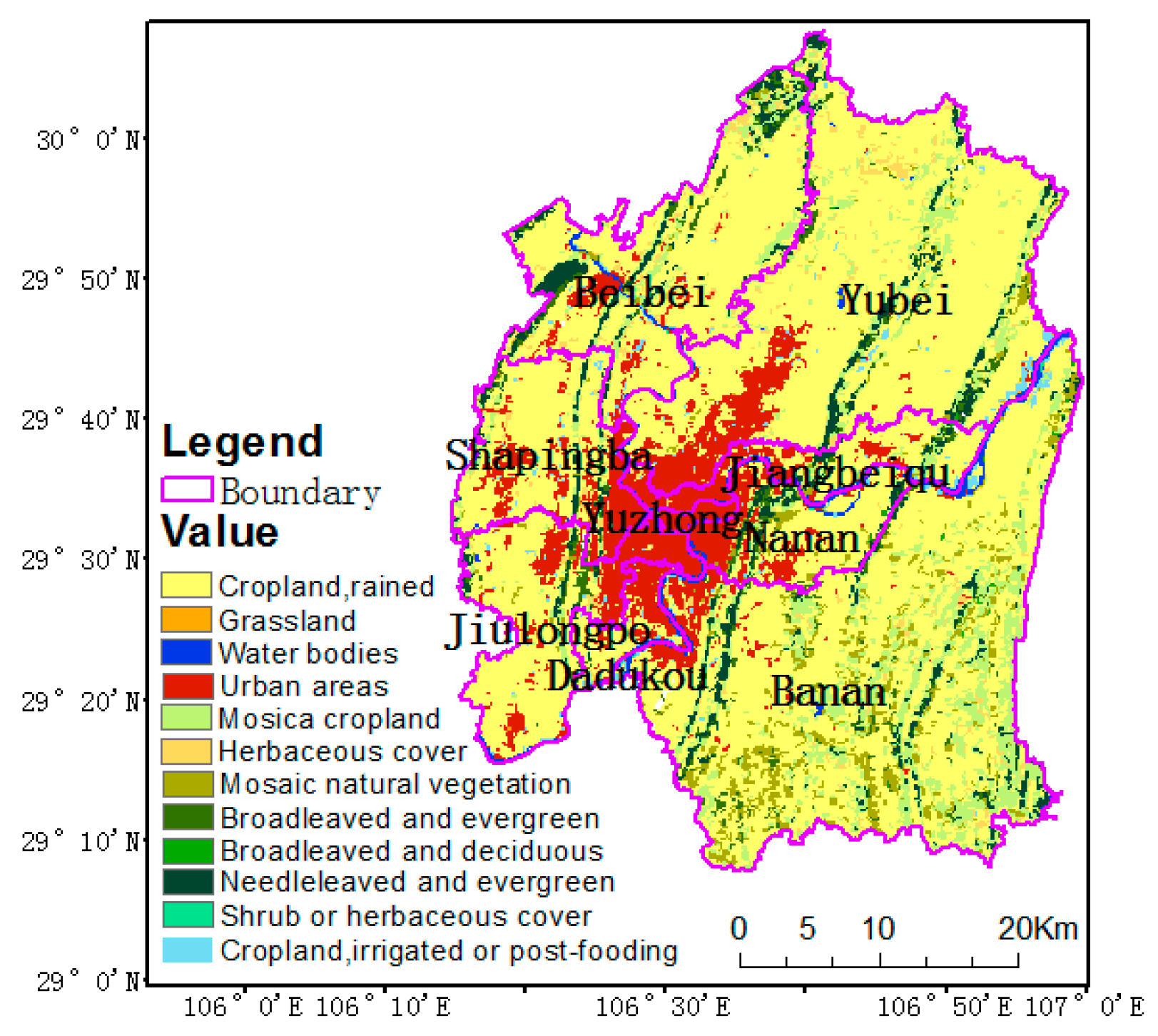
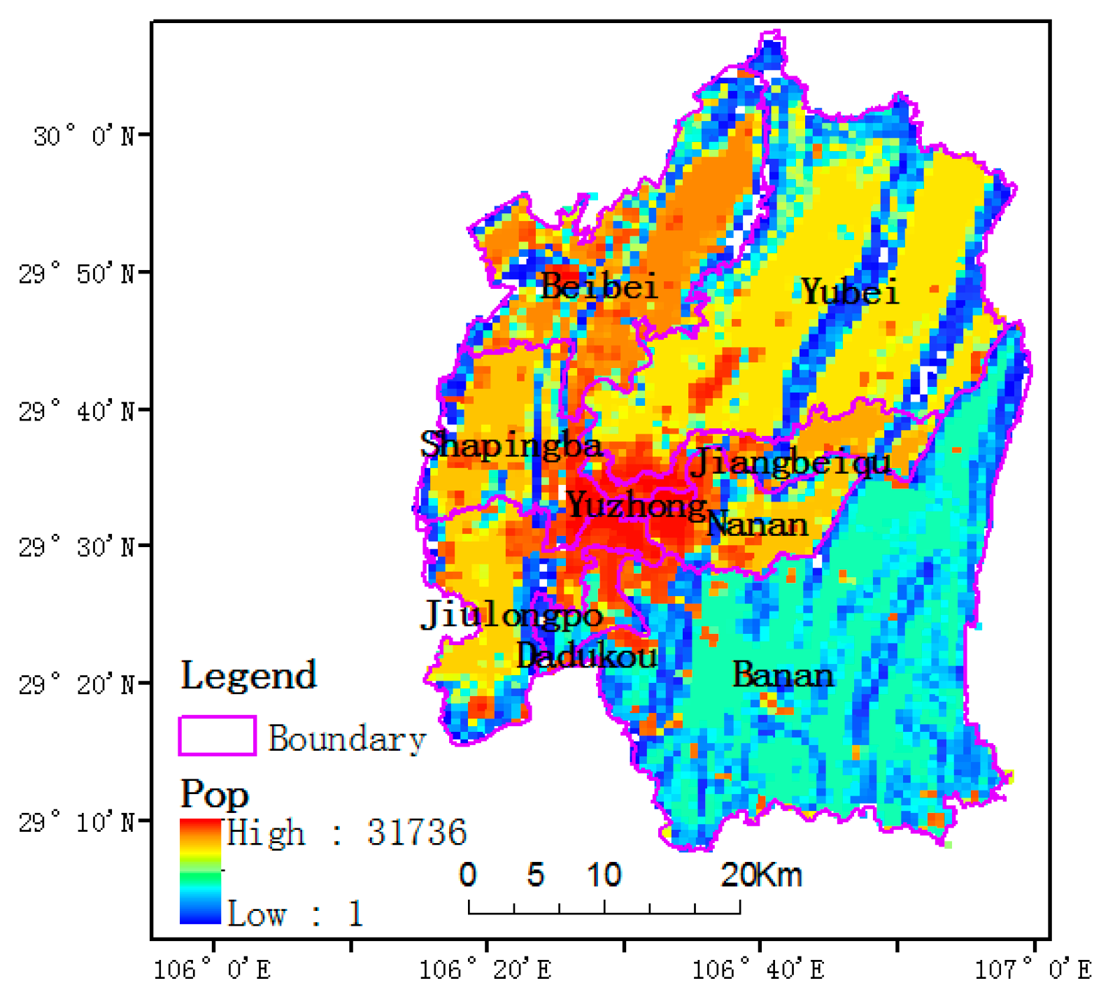
2.1. Study Area

As shown in Figure 1, the study area is the major urban areas of Chongqing (including nine districts, namely Beibei, Yubei, Jiangbei, Shapingba, Yuzhong, Nan’an, Jiulongpo, Dadukou, and Banan), and locates in the southwest of China and the upper reaches of Yangtze River. It covers an area of 5473 km2 and holds a large population of about 8.35 million. The entire urban area is developed on a terrain of hill land, and is mainly surrounded by Liangshan and Zhenwu mountains. Low wind speed and high humidity are prevalent in this region, which further decreases the diffusion of local air pollutants.

2.2. Data

2.2.1. Satellite-Retrieved AOD Data

FY-3C was launched on 23 September 2013, which is the third of the second-generation polar-orbital meteorological satellite. As one of the most widely used sensors onboard FY-3C, MERSI contains 20 spectral bands covering the spectrum from 0.42 μm to 12.5 μm, of which five have a resolution of 250 m, and the others are 1 km at nadir. MERSI is designed to research cloud, aerosol, ecology, and surface classification, and the operational product of 1 km AOD over land based on the Dark Target algorithm and was released by NMSC [26]. The study obtains MERSI 1 km AOD products from May 2014 to May 2015, which were selected by using the cloud detection products of the FY3C/VIRR (Visible and InfraRed Radiometer) to eliminate obstructions caused by clouds. Besides, to completely ensure the data quality, AOD values greater than 2.0 were assumed as being contaminated by clouds and therefore were discarded [27]. We obtained ground-measured data from automatic sun tracking spectrophotometer CE-318 (CE-318) located in Chengdu (103.98° E, 30.59° N) from May 2014 to May 2015. The averages of FY3C/AOD data around monitor station were applied with a search radius of 3 km for the matching with CE-318 measurements in cloudless days. Because the matching was conducted during the satellite overpass time, thereby 19 couples of data were obtained, shown in Figure 2. The correlation coefficient is 0.77, and the RMSE and Bias are 0.27 and −0.03, indicating the FY3C/AOD is reliable.

2.2.2. In Situ PM2.5

The ground-level PM2.5 data over the study area from May 2014 to May 2015 was obtained from Chongqing Environmental Protection Bureau (http://data.cma.cn/). There are 17 air quality-monitoring sites in total, of which the locations are marked in Figure 1. There are Xinshancun (JYS), Tangjiatuo (TJT), Gaojiahuayuan (GJHY), Huxi (HX), Yangjiaping (YJP), Baishiyi (BSY), Nanping (NP), Chayuan (CY), Tiansheng (TS), Jinyunshan (JYS), Caijia (CJ), Lianglu (LL), Konggang (KG), Yuxinjie (YXJ), Nanquan (NQ), Lijia (LJ), Jiefangbei (JFB). PM2.5 concentration is measured by the Tapered Element Oscillating Microbalance (TEMO) approach or Beta-attenuation approach, both of which comply with the National Standard for Environmental Air Quality (GB3095-2012) [28]. High ambient humidity right after precipitation usually brings about extremely small or even negative PM2.5 concentrations, thus the data obtained with 1 h after the precipitation would not be used for modeling. The performance of a statistical model linking satellite AOD to ground-level PM2.5 can be influenced by the temporal resolution of input data [29]. Therefore, the average PM2.5 of one hour before and after the satellite overpass time is calculated as the input to the further analysis.

2.2.3. Meteorological Data

Meteorological data are found to be helpful for improving modeling performance [16,30,31,32]. For example, surface pressure (PS) can influence atmospheric stability and vertical dispersion of air pollution, wind speed (WS) can affect the horizontal transport of air pollutants, relative humidity (RH) and temperature (TMP) mainly relate to particle compositions. Therefore, four meteorological parameters, including RH, TMP, PS, and WS, were collected at five meteorological stations that they locate in Beibei, Jiangbei, Chongqing, Baxian, and Bishan, respectively. Yellow asterisks represent meteorology stations’ geographic position in Figure 1. All meteorology data were retrieved from the China Meteorological Data Sharing Service System (CMDSSS on http://data.cma.cn/), and the temporal resolution is 1 h. In order to achieve a precise matching, the averaged meteorological data temporally near the satellite overpass time (less than one hour) were calculated. The number of meteorological monitors did not match the number of PM2.5 stations, thereby we used the Co-kriging interpolation method to interpolate meteorological data, and the elevation was used as the covariate in interpolation process [33,34,35]. Additionally, the interpolation result was resampled with finer spatial resolutions of 1 km × 1 km and 10 km × 10 km to be consistent with the spatial resolutions of FY3C and MODIS, respectively. We marked 1 km buffer around each meteorological station. If the PM2.5 station was within the buffer zone, the meteorological station information was used, otherwise the interpolation result was used. Because it is difficult to obtain real-time boundary layer height (PBL), the seasonal averaged boundary layer height over the study area were employed, namely 1076 m for spring, 1880 m for summer, 1358 m for autumn and 1061 m for winter, respectively [36].

2.2.4. Auxiliary Data

Chongqing is located on a hill land terrain. The surface types, the elevation, and population density might also affect the AOD-PM2.5 correlation [27]. For example, there are mainly sulfates and nitrates in urban areas because of the factories and vehicles. In rural areas, it is mainly nitrate and organic carbon from biomass burning. Sulfate particles generally have higher light extinction efficiency than carbonaceous particle especially under high relative humidity conditions [37]. The population density is related to emissions, and the increase population density lead to carbon emission to show a downward trend and then an upward trend. The composition was influenced the PM2.5 and lead the Aerosol scattering difference [38]. The elevation has influenced meteorological factors, while different meteorological factors are related to the PM2.5-AOD correlation. The elevation data of the study area were obtained from Shuttle Radar Topographic Mission (SRTM on http://srtm.csi.cgiar.org/), of which the spatial resolution is about 90 m. GlobCover, a 300 m land cover product provided by European Space Agency (ESA), was collected for the year of 2015 (http://due.esrin.esa.int/). Population density at 1-km resolution for 2010 was downloaded from the Data Center for Resource and Environmental Sciences, Chinese Academy of Sciences (http://www.resdc.cn). Since the original projections and spatial resolutions of the datasets varied largely, all the datasets were re-projected to the WGS-84 coordinate system and were resampled to 1 km × 1 km by ARCGIS. The nearest neighbor method was used in the resampling process (shown in Figure 1, Figure 3 and Figure 4, respectively), to be directly matched to MERSI AOD.

2.3. The Combined Mixed Effect Model

2.3.1. Model Description

The AOD-PM2.5 correlation is not only determined by the aerosol composition, vertical profile and meteorological factors [29], but also varies fast over time. As an extension of the general linear models, LME model accounts for both of the fixed effects and the random effects, which enables LME to better explain the temporal relationship between AOD and PM2.5 [13]. By considering the parameters discussed in this study, the initial LME model is developed as Equation (1) termed as Model I:
P M 2.5 , s t = ( α + ω ) + ( β 1 + u 1 ) × A O D s t + ( β 2 + u 2 ) × T M P s t + ( β 3 + u 3 ) ×   R H s t      + ( β 4 + u 4 ) × W S s t + ( β 5 + u 5 ) × P S s t + β 6 × E L E V s + β 7 ×   P o p s      + ε s t
where P M 2.5 , s t is the dependent variable, and A O D s t , T M P s t , R H s t , W S s t , and P S s t are the independent variables for the grid s on day t, respectively.   E L E V s is elevation values (m) at site s;   P o p s is population density (ten thousand/km2) at site s. α, ω, β and u are fitting coefficients, and ε s t stands for the residual error. Descriptions of all the model input and fitting coefficients are recorded in Table 1.
Tian et al. proposed a semi-empirical model to characterize the non-linearity relationship between AOD and PM2.5 [39]. AOD and WS approximately exhibit as power functions of PM2.5, while TMP and RH usually show an exponential relationship with PM2.5 [29]. Therefore, a semi-empirical model considering these non-linear impacts is integrated into Equation (1), forming a new combined model as Equation (2).
P M 2.5 = e ( α + ω ) + ( β 2 + u 2 ) × T M P + ( β 3 + u 3 ) × R H + ( β 4 + u 4 ) × P S × A O D ( β 1 + u 1 ) × ( W S ) β 5 + β 5  
Both sides of Equation (2) are then log-transformed to achieve a linear regression form, shown as Equation (3), so as to promote parameterization and to reduce the skewness of data distribution [29,39]:
ln ( P M 2.5 ) = ( α + ω ) + ( β 1 + u 1 ) × ln ( AOD ) + ( β 2 + u 2 ) × T M P + ( β 3 + u 3 ) × R H + ( β 4 + u 4 ) × P S + ( β 5 + u 5 ) × ln ( W S )  
Song et al. employed a general linear model and a semi-empirical model to compare the relationship between AOD and PM2.5 in the Pearl River delta region using MODIS AOD products, and the results showed that the semi-empirical model was better than the empirical model [18]. Therefore, the paper proposes that the semi-empirical model is integrated into the line mixed effect model based on the study by Song, which expresses the continuous change over time between AOD and PM2.5, in order to improve the accuracy of regression model. The Mode II can be expressed as Equation (4):
ln ( P M 2.5 , s t ) = ( α + ω ) + ( β 1 + u 1 ) × ln ( A O D s t ) + ( β 2 + u 2 ) × T M P s t + ( β 3 + u 3 ) × R H s t + ( β 4 + u 4 ) × P S + ( β 4 + u 4 ) × ln ( W S s t ) + β 5 × E L E V s + β 6 × P o p s + ε s t
Parameters are listed Table 1.

2.3.2. Model Validation

A 10-fold cross-validation (CV) method was used to test the model’s performance in order to avoid the over-fitting. Theory of CV is that the entire model-fitting dataset is randomly split into 10 subsets, and the number of each subset is approximately 10% of the total data records. In each round of cross validation, 10% of the data is select as testing samples and the remaining nine subsets are used to fit the model. The process is repeated 10 times in turn, and each predicted value is recorded. The average of all the ten times is the result of CV. To evaluate the performance of the fitting model, the Root Mean Squared Error (RMSE), Mean Prediction Error (MPE) and R2 are computed for observed and estimated PM2.5 concentration.

3. Results and Discussion

3.1. Statistical Analysis

The histogram of the probability density distribution and the summary statistics of all the model variables are presented in Figure 5. According to the matched data sample, the mean and maximum values for MERSI AOD and PM2.5 are 0.68 and 0.93, and 50 μg/m3 and 282 μg/m3, respectively. The similarity of the histogram distribution between PM2.5 and AOD indicates high relevance between them. The surface pressure is relatively low, which might be explained as follows: (1) the surface pressure is lower in summer than winter, and most data used in this study is in summer; (2) The average elevation is relatively higher in Chongqing. The major urban areas of Chongqing have relatively humid and stagnant ambient air, with the mean RH and WS of 51.24% and 1.46 m/s, respectively.

3.2. Model Fitting and Validation

Figure 6 exhibits the results of the cross validation (CV) of Model I and Model II. The fitting and validation performance results are given in Table 2. Model II (Figure 6b) performs better than Model I (Figure 6a) with a slightly higher R2 and lower RMSE and MPE, which demonstrates an overall improvement in the estimation of PM2.5 from AOD by integrating the semi-empirical model in to LME. Due to limited data available during winter, all the data samples in this study are divided into a warm season (from April to September) and a cold season (from October to March), no matter the observations were obtained in continuous monthly sequence or not. Model II is applied to both of the seasons of data, and the fitting results are shown in Figure 6c,d. Based on comparing the correlation level, Model II performed relatively better in the cold season than in the warm season, while the RMSE and MPE are higher in the cold season. One of the possible reason is that, more precipitation and more humid air in the warm season favor the hygroscopic growth of particles, which might lead to the distribution of aerosol particle size and the change of composition [40]. This might bring additional uncertainties into the AOD-PM2.5 relationship. There is high PM2.5 concentration in cold seasons, which leads to high RMSE and MPE. Compared to the relevant model fitting, the CV results can have slightly lower correlation R2 and higher RMSE, indicating that over-fittings existed in both Model I and Model II. The reason of this result can be that the Linear Mixed Effects model is similar to the black box model [41]. It cannot completely make clarify the relation of PM2.5 to AOD and meteorological factors, which leads to the over-fitting in the Model I and Model II.
Figure 7 presents the comparison between the satellite estimated and the in situ mean PM2.5 concentrations during the whole study period over each air quality site, which indicates that the combined model in this study performs homogenously well over the urban area in Chongqing. In general, JFB, GJHY and BSY, all of which are located in the most commercial and populated part of the urban area, have relatively high level of PM2.5. Among all these sites, the lowest annual mean PM2.5 of 38.6 μg/m3 was found in JYS, which is far from the major urban areas of Chongqing and located in a national protected natural area.

3.3. Spatial Distribution of Estimated PM2.5

Figure 8a–c respectively present the spatial distribution of mean PM2.5 in the cold seasons, the warm seasons, and the whole study period, all of which were estimated from MERSI AOD using Model II. Overall, similar spatial patterns are found in these three periods. High PM2.5 values mostly concentrated over Yuzhong, the most urbanized and populated part of the study area, while Banan and the southeastern part of Yubei, which are mainly covered by vegetation and have much less population, have the lowest PM2.5 level. The spatial distribution of PM2.5 indicates that the local anthropogenic emissions contribute to most of air pollution. The main sources of PM2.5 in these region are vehicles exhaust and secondary particles such as sulfates and nitrates [42]. In general, regional PM2.5 is higher in the cold seasons than the warm seasons, particularly in Yubei and Banan, which is consistent with the previous research [22]. It should be noted that, as shown in Figure 8a–c, PM2.5 concentration over waters was somehow overestimated, and this bias may be mostly associated to more humid air, which probably causes abnormally high retrievals of MERSI AOD.
To demonstrate the advantage of estimating PM2.5 using MERSI AOD, the 10 km × 10 km Level 2 MODIS AOD product matching to the data samples of this study is employed to estimate PM2.5 using Model II. We calculated the annual average PM2.5 concentration by using MODIS products, and the data were resampled to 1 km × 1 km in order to compare with MERSI, which is presented in Figure 8d. It exhibits overall spatial consistence with the estimated PM2.5 by MERSI. Compared to MODIS, the finer resolution of MERSI provides much more detailed information of PM2.5 distribution, especially over the densely populated areas. This is very helpful to evaluate PM2.5’s impact on public health at urban scale, and can also improve the effect of local emission control. Since estimation are based on the same model, the differences between MERSI PM2.5 and MODIS PM2.5 are basically caused by the difference in their AOD, which can be attributed to spatial resolution, overpass time and channel spectrum.
In Figure 9, the upper subplots show the true-color images, and we selected no-cloud days from four seasons, namely 30 July 2014 for summer, 10 September 2014 for fall, 12 February 2015 for winter, and 28 April 2015 for spring, respectively, which could be observed from true-color and FY3C/VIRR cloud products that was not depicted in the paper. The lower subplots were the calculated PM2.5 concentration using Model II. These data indicate that the FY3C/MERSI could be used to retrieve high resolution PM2.5 in no-cloud conditions. According to the in situ measurements at the ground sites, the area-averaged PM2.5 concentrations of the four days are 28.07 μg/m3, 65.09 μg/m3, 112.41 μg/m3, and 97.64 μg/m3, respectively. Instead, the continuous distribution of PM2.5 estimated by MERSI provides detailed spatial pattern of regional air quality, which might not be clearly described by sparse ground-level observations.

4. Conclusions

In this study, the 1 km AOD retrieved by MERSI onboard FY-3C satellite was employed to estimate the ground-level PM2.5 over the main urban area in Chongqing, one of the significant metropolitan city in China. To better account for the complex atmospheric and topographical conditions in Chongqing, an advanced statistical model is developed to convert MERSI AOD into PM2.5 concentration, which comprehensively considers the impact of several meteorological and environmental parameters. This model is achieved by integrating a semi-empirical model into a mixed effect model, and performs better than a single LME model in predicting PM2.5 during the whole study period. In addition, the data samples of this study were divided into the cold seasons and the warm seasons. Satellite estimates show higher PM2.5 levels in the cold seasons than in the warm seasons over most of the study area, which agree with the result of local in situ observations.
A clear spatial pattern of ground-level PM2.5 in the major urban areas of Chongqing is depicted by MERSI observations. High PM2.5 levels mainly occur in Yuzhong, the most urbanized and populated district of the city and much lower PM2.5 is found in vegetated suburban areas, such as Banan and Yubei. This indicates that the air pollution in the major urban areas of Chongqing is mainly contributed by local emissions. Furthermore, the 10 km Level MODIS AOD was used to estimate PM2.5 and compared with MERSI estimation, which clearly demonstrates the advantages of high resolution MERSI observations in characterizing detailed spatial distribution of local air pollution.
Though promising PM2.5 estimation has been achieved in this study, our combined statistical model still needs to be improved. Daily or even hourly PBL retrieved by LIDAR or simulated by numerical models will help to better account for the influence of aerosol vertical distribution. We will extend the numbers of years of study to account for meteorological variability from year to year when the satellite can detect more data.

Acknowledgments

This study was supported by the National key Research and Development Program of China (Grant No. 2016YFC0200404), the National Natural Science Foundation of China (Grant No. 41571347), the Open Foundation of Chongqing Meteorology (KFJJ201402) and the Education Department Innovation team in Sichuan (16TD0024). The authors are grateful to the FY-3C (http://satellite.nsmc.org.cn), MODIS (https://lance.modaps.eosdis.nasa.gov/), Chongqing Environmental Protection Bureau (http://data.cma.cn/), CMDSSS (http://data.cma.cn/), SRTM (http://srtm.csi.cgiar.org/), European Space Agency (ESA) (http://due.esrin.esa.int/), and the Data Center for Resource and Environmental Sciences, Chinese Academy of Sciences (http://www.resdc.cn) scientific team for the provision of satellite data and situ measurement data utilized in this study.

Author Contributions

Qiaolin Zeng proposed the method, collected data, and wrote this paper; Zifeng Wang and Jinhua Tao conceived of the experiment and revised the paper; Yongqian Wang, Liangfu Chen, Hao Zhu, Yang Jie, and Xinhui Wang provided technical guidance and revised the paper; Bin Li offered technical guidance for the FY-3C AOD data.

Conflicts of Interest

The authors declare no conflict of interest.

References

  1. Bell, M.L.; Keita, E.; Kathleen, B. Ambient Air Pollution and Low Birth Weight in Connecticut and Massachusetts. Environ. Health Perspect. 2007, 115, 1118–1124. [Google Scholar] [CrossRef] [PubMed]
  2. Dominici, F.; Peng, R.D.; Bell, M.L.; Pham, M.L.; Mcdermott, A.; Zeger, S.L.; Samet, J.M. Fine particulate air pollution and hospital admission for cardiovascular and respiratory diseases. J. Am. Med. Assoc. 2006, 295, 1127–1134. [Google Scholar] [CrossRef] [PubMed]
  3. Slama, R.; Morgenstern, V.; Cyrys, J.; Zutavern, A.; Herbarth, O.; Wichmann, H.E.; Heinrich, J.; Group, T.L.S. Traffic-related atmospheric pollutants levels during pregnancy and offspring’s term birth weight: A study relying on a land-use regression exposure model. Environ. Health Perspect. 2007, 115, 1283–1292. [Google Scholar] [CrossRef] [PubMed]
  4. Hutchison, K.D. Applications of MODIS satellite data and products for monitoring air quality in the state of Texas. Atmos. Environ. 2003, 37, 2403–2412. [Google Scholar] [CrossRef]
  5. Falke, S.R.; Husar, R.B.; Schichtel, B.A. Fusion of SeaWIFS and TOMS satellite data with surface observations and topographic data during extreme aerosol events. J. Air Waste Manag. Assoc. 2001, 51, 1579–1585. [Google Scholar] [CrossRef] [PubMed]
  6. Van Donkelaar, A.; Martin, R.V.; Brauer, M.; Boys, B.L. Use of satellite observations for long-term exposure assessment of global concentrations of fine particulate matter. Environ. Health Perspect. 2015, 123, 135–143. [Google Scholar] [CrossRef] [PubMed]
  7. Liu, Y. New directions: Satellite driven PM2.5 exposure models to support targeted particle pollution health effects research. Atmos. Environ. 2013, 68, 52–53. [Google Scholar] [CrossRef]
  8. Liu, Y. Monitoring PM2.5 from space for health: Past, present, and future directions. Environ. Manag. 2014, 6, 6–10. [Google Scholar]
  9. Chu, D.A.; Tsai, T.C.; Chen, J.P.; Chang, S.C.; Jeng, Y.J.; Chiang, W.L.; Lin, N.H. Interpreting aerosol LiDAR profiles to better estimate surface PM2.5 for columnar AOD measurements. Atmos. Environ. 2013, 79, 172–187. [Google Scholar] [CrossRef]
  10. Zhang, Y.; Li, Z. Remote sensing of atmospheric fine particulate matter (PM2.5) mass concentration near the ground from satellite observation. Remote Sens. Environ. 2015, 160, 252–262. [Google Scholar] [CrossRef]
  11. Wang, J. Intercomparison between satellite-derived aerosol optical thickness and PM2.5 mass: Implications for air quality studies. Geophys. Res. Lett. 2003, 30, 2029. [Google Scholar] [CrossRef]
  12. Hoff, R.M.; Christopher, S.A. Remote sensing of particulate pollution from space: Have we reached the promised land? J. Air Waste Manag. Assoc. 2009, 59, 645–675. [Google Scholar] [PubMed]
  13. Lee, H.J.; Liu, Y.; Coull, B.A.; Schwartz, J.; Koutrakis, P. A novel calibration approach of modis AOD data to predict PM2.5 concentrations. Atmos. Chem. Phys. 2011, 11, 9769–9795. [Google Scholar] [CrossRef]
  14. Hu, X.; Waller, L.A.; Al-Hamdan, M.Z.; Crosson, W.L.; Estes, M.G.; Estes, S.M.; Quattrochi, D.A.; Sarnat, J.A.; Liu, Y. Estimating ground-level PM2.5 concentrations in the southeastern U.S. using geographically weighted regression. Environ. Res. 2013, 121, 1–10. [Google Scholar] [CrossRef] [PubMed]
  15. Liu, Y.; Sarnat, J.A.; Kilaru, V.; Jacob, D.J.; Koutrakis, P. Estimating ground-level PM2.5 in the eastern united states using satellite remote sensing. Environ. Sci. Technol. 2005, 39, 3269–3278. [Google Scholar] [CrossRef] [PubMed] [Green Version]
  16. Liu, Y.; Paciorek, C.J.; Koutrakis, P. Estimating regional spatial and temporal variability of PM2.5 concentrations using satellite data, meteorology, and land use information. Environ. Health Perspect. 2009, 117, 886–892. [Google Scholar] [CrossRef] [PubMed] [Green Version]
  17. Hu, X.; Waller, L.A.; Lyapustin, A.; Wang, Y.; Liu, Y. Improving satellite-driven PM2.5 micrometer models with moderate resolution imaging spectroradiometer fire counts in the southeastern U.S. J. Geophys. Res. Atmos. 2014, 119. [Google Scholar] [CrossRef] [PubMed]
  18. Song, W.; Jia, H.; Huang, J.; Zhang, Y. A satellite-based geographically weighted regression model for regional PM2.5 estimation over the Pearl River Delta region in China. Remote Sens. Environ. 2014, 154, 1–7. [Google Scholar] [CrossRef]
  19. You, W.; Zang, Z.; Zhang, L.; Li, Y.; Pan, X.; Wang, W. National-scale estimates of ground-level PM2.5 concentration in China using geographically weighted regression based on 3 km resolution modis AOD. Remote Sens. 2016, 8, 184. [Google Scholar] [CrossRef]
  20. Li, S.; Joseph, E.; Min, Q. Remote sensing of ground-level PM2.5 combining AOD and backscattering profile. Remote Sens. Environ. 2016, 183, 120–128. [Google Scholar] [CrossRef]
  21. Remer, L.A.; Kaufman, Y.J.; Tanré, D.; Mattoo, S.; Chu, D.A.; Martins, J.V.; Li, R.-R.; Ichoku, C.; Levy, R.C.; Kleidman, R.G.; et al. The MODIS aerosol algorithm, products, and validation. J. Atmos. Sci. 2005, 62, 947–973. [Google Scholar] [CrossRef]
  22. Deng, Y.; Hu, M.; Lin, C.; Cao, J. Analysis on the air quality status and meteorological condition of Chongqing urban area in 2015. Sichuan Environ. 2016, 42, 61–66. (In Chinese) [Google Scholar]
  23. Ge, Q.; Hu, Y.; Zhang, L.; Zhang, S. Retrieval of aerosol over land surface from FY-3C/MERSI with DDV algorithm. Remote Sens. Inf. 2017, 32, 34–38. [Google Scholar]
  24. Teng, W. Retrieval of Aerosol over Beijing and Sorround Using MERSI and MODIS Data. Master’s Thesis, Capital Normal University, Beijing, China, 2013. (In Chinese). [Google Scholar]
  25. Zhou, Y.; Bai, J.; Zhou, Z.; Qi, L. Aerosol optical depth retrieval from FY-3A/MERSI for sand-dust weather over ocean. J. Remote Sens. 2014, 18, 771–787. [Google Scholar]
  26. Kaufman, Y.J.; Tanré, D.; Remer, L.A.; Vermote, E.F.; Chu, A.; Holben, B.N. Operational remote sensing of tropospheric aerosol over land from EOS moderate resolution imaging spectroradiometer. J. Geophys. Res. Atmos. 1997, 102, 17051–17067. [Google Scholar] [CrossRef]
  27. Hu, X.; Waller, L.A.; Lyapustin, A.; Wang, Y.; Al-Hamdan, M.Z.; Crosson, W.L.; Estes, M.G.; Estes, S.M.; Quattrochi, D.A.; Puttaswamy, S.J.; et al. Estimating ground-level PM2.5 concentrations in the southeastern united states using MAIAC AOD retrievals and a two-stage model. Remote Sens. Environ. 2014, 140, 220–232. [Google Scholar] [CrossRef]
  28. OuYang, S. Summarization on PM2.5 online monitoring technique. China Environ. Prot. Ind. 2012, 4, 14–18. (In Chinese) [Google Scholar]
  29. Liu, Y.; Franklin, M.; Kahn, R.; Koutrakis, P. Using aerosol optical thickness to predict ground-level PM2.5 concentrations in the St. Louis area: A comparison between MISR and MODIS. Remote Sens. Environ. 2007, 107, 33–44. [Google Scholar] [CrossRef]
  30. Gupta, P.; Christopher, S.A.; Wang, J.; Gehrig, R.; Lee, Y.; Kumar, N. Satellite remote sensing of particulate matter and air quality assessment over global cities. Atmos. Environ. 2006, 40, 5880–5892. [Google Scholar] [CrossRef]
  31. Barman, S.C.; Singh, R.; Negi, M.P.S.; Bhargava, S.K. Fine particles (PM2.5) in residential areas of lucknow city and factors influencing the concentration. CLEAN Soil Air Water 2010, 36, 111–117. [Google Scholar] [CrossRef]
  32. Pateraki, S.; Asimakopoulos, D.N.; Flocas, H.A.; Maggos, T.; Vasilakos, C. The role of meteorology on different sized aerosol fractions (PM10, PM2.5, PM2.5–10). Sci. Total Environ. 2012, 419, 124–135. [Google Scholar] [CrossRef] [PubMed]
  33. Liu, Y.; Chen, P.Q.; Zhang, W.; Hu, F. A spatial interpolation method for surface air temperature and its error analysis. Chin. J. Atmos. Sci. 2006, 30, 146–152. (In Chinese) [Google Scholar]
  34. Tang, G.A.; Zhao, M.D.; Yang, X.; Zhou, Y. Geographic Information System; Science Press: Beijing, China, 2002. [Google Scholar]
  35. Jiang, X.J.; Liu, X.J.; Huang, F.; Jiang, H.Y.; Cao, W.X.; Zhu, Y. Comparison of spatial interpolation methods for daily meteorological elements. Chin. J. Appl. Ecol. 2010, 21, 624–630. (In Chinese) [Google Scholar]
  36. Zheng, Z.; Chen, L.; Zheng, J.; Zhong, L. Application of retrieved high-resolution AOD in regional pm monitoring in the pearl river delta and Hong Kong region. Acta Sci. Circumst. 2011, 31, 1154–1161. [Google Scholar]
  37. Chin, M. Tropospheric aerosol optical thickness from the gocart model and comparisons with satellite and sun photometer measurements. J. Atmos. Sci. 2002, 59, 461–483. [Google Scholar] [CrossRef]
  38. Li, S.L. Density of population, industrial structure and quality of urbanization. Commer. Res. 2014, 12, 61–67. [Google Scholar]
  39. Tian, J.; Chen, D. A semi-empirical model for predicting hourly ground-level fine particulate matter (PM2.5) concentration in southern Ontario from satellite remote sensing and ground-based meteorological measurements. Remote Sens. Environ. 2010, 114, 221–229. [Google Scholar] [CrossRef]
  40. Malm, W.C.; Day, D.E.; Kreidenweis, S.M. Light scattering characteristics of aerosols as a function of relative humidity: Part I—A comparison of measured scattering and aerosol concentrations using the theoretical models. J. Air Waste Manag. Assoc. 2000, 50, 686–700. [Google Scholar] [CrossRef] [PubMed]
  41. Ma, Z. Study on Spatiotemporal Distributions of PM2.5 in China Using Satellite Remote Sensing. Ph.D. Thesis, Nanjing University, Nanjing, China, 2015. (In Chinese). [Google Scholar]
  42. Chen, Y.; Xie, S.; Luo, B.; Zhai, C. Pollution characterization and source apportionment of fine particles in urban Chongqing. Acta Sci. Circumst. 2017, 37, 2420–2430. (In Chinese) [Google Scholar]
Figure 1. Study area and Locations of the 17 environment monitoring sites denoted by numbers (1. Xinshancun; 2. Tangjiatuo; 3. Gaojia; 4. Huxi; 5. Panjiaping; 6. Baishiyi; 7. Nanping; 8. Caiyuan; 9. Tiansheng; 10. Jinyunshan; 11. Caijia; 12. Lianglu; 13. Konggang; 14. Yuxinjie; 15. Nanquan; 16. Lijia; and 17. Jiefangbei), and 5 meteorology stations (a. Beibei; b. Jiangbei; c. Chongqing; d. Baxian; e. Bishan).
Atmosphere 09 00003 g001
Figure 2. The verification of FY3C/AOD and CE318, the data obtained from May 2014 to May 2015.
Atmosphere 09 00003 g002
Figure 3. Land use types distribution in 2015.
Atmosphere 09 00003 g003
Figure 4. Population density distribution in 2010.
Atmosphere 09 00003 g004
Figure 5. Histograms and descriptive statistics of all dependent and independent variables included in the model fitting data set (N = 1106). (a) fine particulate matter (PM2.5); (b) aerosol optical depth (AOD); (c) relative humidity (RH); (d) surface pressure (PS); (e) urface temperature (Tmp); (f) wind speed (wind).
Atmosphere 09 00003 g005
Figure 6. Scatter plot of cross-validated values in Model I and Model II. (a) is Model I CV result to overall data; (b) is Model II CV result to overall data; (c) is Model II CV result to cold season data; (d) is Model II CV result to overall data. The black line shows the 1:1 line as a reference, the red line shows the regression line.
Atmosphere 09 00003 g006
Figure 7. The mean and residuals by observing and fitting PM2.5 at each station.
Atmosphere 09 00003 g007
Figure 8. The spatial distribution of average PM2.5 estimated concentration by FY-3C/MERSI in cold seasons (a), warm seasons (b), and the annual average (c), respectively; (d) represents the annual average PM2.5 concentration by MODIS.
Atmosphere 09 00003 g008
Figure 9. The true color (ad) and PM2.5 concentration (eh) on 30 July 2014, 10 September 2014, 12 February 2015, and 28 April 2015, in sequence.
Atmosphere 09 00003 g009
Table 1. Definitions of independent variables used in Equations (1)–(4).
VariableUnitDescription
AODUnit lessFY-3C MERSI AOD
TMP°CTemperature
WSm/sWind Speed
RH%Relative humidity
PShPaSurface pressure
ELEVmElevation
PopTen thousand/km2Population density
αUnit lessFixed effects intercept
ωUnit lessRandom effects intercept
β1–β5Unit lessFixed effects slope
u1–u5Unit lessRandom effects slope
εUnit lessRandom errors
Table 2. Describing statistical model fitting and CV results (Sit number = 17).
NameParametersModel I (All Data)Model II (All Data)Model II (Warm)Model II (Cold)
FittingN11061106838268
R20.890.900.810.92
RMSE (μg/m3)12.2711.419.1713.51
MPE (μg/m3)7.857.626.3710.43
CVR20.850.870.790.88
RMSE (μg/m3)13.7212.099.7315.86
RMSE (μg/m3)9.178.927.4813.51

