Extreme Rainfall and Flooding over Central Kenya Including Nairobi City during the Long-Rains Season 2018: Causes, Predictability, and Potential for Early Warning and Actions

Abstract

The Long-Rains wet season of March–May (MAM) over Kenya in 2018 was one of the wettest on record. This paper examines the nature, causes, impacts, and predictability of the rainfall events, and considers the implications for flood risk management. The exceptionally high monthly rainfall totals in March and April resulted from several multi-day heavy rainfall episodes, rather than from distinct extreme daily events. Three intra-seasonal rainfall events in particular resulted in extensive flooding with the loss of lives and livelihoods, a significant displacement of people, major disruption to essential services, and damage to infrastructure. The rainfall events appear to be associated with the combined effects of active Madden–Julian Oscillation (MJO) events in MJO phases 2–4, and at shorter timescales, tropical cyclone events over the southwest Indian Ocean. These combine to drive an anomalous westerly low-level circulation over Kenya and the surrounding region, which likely leads to moisture convergence and enhanced convection. We assessed how predictable such events over a range of forecast lead times. Long-lead seasonal forecast products for MAM 2018 showed little indication of an enhanced likelihood of heavy rain over most of Kenya, which is consistent with the low predictability of MAM Long-Rains at seasonal lead times. At shorter lead times of a few weeks, the seasonal and extended-range forecasts provided a clear signal of extreme rainfall, which is likely associated with skill in MJO prediction. Short lead weather forecasts from multiple models also highlighted enhanced risk. The flood response actions during the MAM 2018 events are reviewed. Implications of our results for forecasting and flood preparedness systems include: (i) Potential exists for the integration of sub-seasonal and short-term weather prediction to support flood risk management and preparedness action in Kenya, notwithstanding the particular challenge of forecasting at small scales. (ii) We suggest that forecasting agencies provide greater clarity on the difference in potentially useful forecast lead times between the two wet seasons in Kenya and East Africa. For the MAM Long-Rains, the utility of sub-seasonal to short-term forecasts should be emphasized; while at seasonal timescales, skill is currently low, and there is the challenge of exploiting new research identifying the primary drivers of variability. In contrast, greater seasonal predictability of the Short-Rains in the October–December season means that greater potential exists for early warning and preparedness over longer lead times. (iii) There is a need for well-developed and functional forecast-based action systems for heavy rain and flood risk management in Kenya, especially with the relatively short windows for anticipatory action during MAM.

1. Introduction

1.1. Climate Risks in Kenya

East Africa is prone to climate and weather extremes with a highly variable climate, and has relatively high levels of population exposure and vulnerability. In the past few years, the region has experienced both significant drought and flood events. The most notable droughts were during 2015–2016 over Northern Ethiopia and 2016–2017 in the Greater Horn of Africa, including Kenya, associated with El Nino and La Nina conditions, respectively [1,2]. Notable recent flooding includes that during March–May 2018 over much of Kenya, which is the subject of this paper. Regarding flooding in particular, based on the Emergency Events Database (EM-DAT), in recent decades, Kenya experienced major flood events roughly every two years on average, typically affecting about 70,000 people per event [3]. Kenya recorded 17 major flood events between 1964–2004. Flood events with particularly high impact occurred in 1961, 1997–1998, 2006, 2012, and 2018 [3]. The 1997–1998 event cost at least USD $870 million [4]—the equivalent of approximately 11% of the country’s gross domestic product (GDP) [5]—from damages to water systems, roads, communications, and buildings; the costs of treatment for waterborne diseases; and crop loss, which affected more than half a million people [6]. On average, the country experiences a flood that costs about 5.5% of its GDP every seven years [5]. Of course, it must be noted that heavy rainfall and even flooding brings subsequent societal benefits through increased crop yields, fodder for livestock, and the replenishment of surface and groundwater resource. Indeed, a post-season assessment of the 2018 March–May rains by the Kenya Food Security Steering Group [7] indicated that the heavy rainfall had reversed some of the pre-existing food security impacts of preceding poor rainfall seasons, with many counties moving back from ‘Crisis’ to ‘Stressed’ status.

Flood risk Early Warning Systems (EWS) have the potential to help mitigate the impact of flood events, but in Kenya, according to the Kenya Meteorological Department (KMD), a flood-specific EWS is currently operational only for a single river basin: the Nzoia river in Western Kenya [8]. Weather/climate forecasts and advisory bulletins with early warnings are provided to the public by KMD (www.meteo.go.ke). However, one review of the public experience of early warnings suggests that lead times are often not sufficient for effective action [9]. Nevertheless, the potential for improved flood EWS in Kenya is supported by improvements in forecasting capability both for weather/climate (e.g., the World Meteorological Organization (WMO) Severe Weather Forecasting Demonstration Project (http://www.wmo.int/pages/prog/www/swfdp/) and for fluvial flood risk (e.g., the Global Flood Awareness System (GLOFAS), www.globalfloods.eu). Moreover, there is increasing interest amongst humanitarian and national agencies in proactive rather than reactive disaster risk management systems based on weather and climate forecasts, including by the recent development of various forecast-based action/finance (FbF/FbA) initiatives [10]. The Forecasts for Preparedness Action (ForPAc) project (www.forpac.org), which supported this study, is one example of a project working toward that objective in Kenya.

This paper aims to explain and quantify the nature, impacts, and large-scale climate drivers of the extreme rainfall over Kenya during March and April 2018, which led to widespread flooding across Kenya, including within Nairobi city itself. We then use this event as a case study to assess the potential for forecasting extreme rainfall over a range of lead times, in order to support early preparedness actions. We draw implications for improving the early warning of extreme rainfall that can potentially cause flooding. The paper is organized as follows: the remainder of Section 1 provides a summary of the drivers and predictability of the Long-Rains over Kenya and East Africa. Section 2 describes data, models, and methods. Section 3 presents the results and discussion, including a descriptive analysis of the extreme rainfall events, their impact, the diagnosis of likely climate drivers, and finally, the evaluation of forecasts over a range of lead times. The implications for EWS and other conclusions are presented in Section 4.

1.2. Climate Drivers of Extreme Rainfall Events during the Long-Rains and the Role of the MJO

Most flood events in Kenya occur during the Long-Rains (March–May, hereafter MAM or LR) or during the Short-Rains (October–December, hereafter OND or SR). Unfortunately, at longer seasonal lead times, the LR season as a whole is far less predictable than the SR [11], as it is less spatially and temporally coherent, and only weakly correlated with most of the main large-scale drivers that control regional climate variability, including El Nino-Southern Oscillation (ENSO) and the Indian Ocean Dipole modes, which are less active during the LR [12]. However, several studies have linked the strong sub-seasonal variability in the LR to the irregular impact of the Madden–Julian Oscillation (MJO) [13,14,15]. Figure 1 shows the typical impacts of the MJO on global tropical rainfall with an eastward propagation of enhanced and suppressed rainfall from the western Indian Ocean (phase 2) toward the Maritime continent (phases 4–5) and the west, central, and east Pacific (phases 6–8). A strong MJO in the Indian Ocean has been linked to a higher frequency of wet spells and enhanced daily rainfall over East Africa during March and April, compared to years when the MJO is weak. This indicates that the amplitude of the MJO can influence seasonal totals and onset [13]. Vellinga and Milton [16] also demonstrate that MAM rainfall is related to the overall seasonal strength of the MJO across all of the phases. However, in detail, the MJO impact over Kenya varies spatially depending on the MJO phase, with wet spells over the highlands occurring during MJO phases 2–4, and over the coastal region throughout phases 6–8 [17]. This variation is attributed to the rainfall-causing mechanisms, and it leads to spatially incoherent rainfall distribution [13]. The physical mechanisms by which the MJO modulates East Africa rainfall are complex, but include both dynamical and thermo-dynamical responses [14]. These are explored in more detail in Section 3.3.

2. Data and Methods

2.1. Observational Data and Analysis

We use a variety of daily rainfall data to ensure robust results. These are:

Daily rainfall from:

Five KMD weather stations in Nairobi County, which calculates the area-averaged using the Thiessen polygon approach to make a Nairobi-wide average over the period 1981–2018.

Climate Hazards InfraRed Precipitation with Station Data (CHIRPS), which is a gridded blended gauge-satellite product [19], to analyze between 1981–2018.

Global Precipitation Climatology Project (GPCP) V1.3 [20], which is a gridded satellite product constrained by monthly gauge precipitation observation, to analyze between 1988–2018.

Monthly rainfall data is obtained from:

The monthly CenTrends rainfall dataset [21] comprising a pooling of station archives, processed onto a 0.1-degree grid from 1900 to 2018.

Global Precipitation Climatology Centre (GPCC) V8.0 gauge-based monthly rainfall dataset [22] covering the period 1891–2018 at one-degree grid resolution.

We examine the extreme rainfall events across spatial scales: the wider East Africa region, and area-averaged rainfall over two boxes centered on 36.75° E, 1.25° S (the approximate location of Nairobi). Specifically, (i) a five-degree box representing the area that experienced the strongest rainfall anomalies, which we refer to as the ‘Kenya core’ rainfall region, and (ii) a 0.5-degree box to represent Nairobi city itself. These study regions are shown in Figure 2.

The return period of daily, five-day, and 10-day rainfall maxima during March and April 2018 is estimated using the block maxima method, in which a generalized extreme value (GEV) distribution is fitted to the distribution of daily/five-day/10-day maxima observed within each month/season/year (using maximum likelihood estimation and a chi-squared goodness-of-fit test). Then, the return periods are estimated by inverting the resulting GEV cumulative probability distribution of block maxima for a range of return periods. As such, the estimated return periods represent the probability of the daily/five-day/10-day maximum observed during March and April 2018 occurring within any March/April month, MAM season, or year. Note that uncertainty in the best estimate of return periods can be quite high for relatively short records, especially for the GPCP data, which extends from 1988.

Information on the large-scale atmospheric circulation during the study period is diagnosed from the horizontal winds and specific humidity from ERA-Interim reanalysis data [23]. We use a simple compositing method to compare the circulation anomalies during the active wet periods within March–April 2018. To analyze MJO activity, we use the standard MJO diagrams of Wheeler and Hendon [24]. These illustrate the phase and amplitude of the MJO based on the principal component time series of the leading two combined Empirical Orthogonal Functions of 850 hPa zonal winds, 200 hPa zonal winds, and satellite outgoing longwave radiation over the global tropics.

2.2. Forecast Model Data

The World Meteorological Organization (WMO) has designated 13 global producing centers (GPCs) of long-range forecasts that are generating operational dynamical-model seasonal forecasts to agreed criteria. A lead center for displaying forecasts in a consistent format and generating multi-model products has also been established: The Lead Centre for Long Range Multi-Model Ensemble (LC-LRFMME) [25]. A number of GPCs are also contributing to the World Weather Research Programme (WWRP)-THORPEX/World Climate Research Programme (WCRP) sub-seasonal to seasonal prediction project (S2S) of the WMO [26]. We examine forecast products for March and April 2018 over a range of lead times, from multiple sources, including the GPCs (with a focus on the European Centre For Medium-Range Weather Forecasts (ECMWF) System5 and Met Office GloSea5 systems [27]) as well as the regional and national forecasting centers, IGAD Climate Prediction and Applications Centre (ICPAC) and KMD, respectively.

2.2.1. Seasonal Forecasts

The seasonal prediction of MAM 2018 is assessed using the WMO LC-LRFMME, the European Centre For Medium-Range Weather Forecasts (ECMWF) seasonal forecast system (SEAS5, hereafter S5) and the Met Office Global Seasonal Prediction System 5 (GloSea5). S5 is a coupled ocean–land–atmosphere prediction system. It makes initialized (once per month) predictions of the global climate system. The atmospheric model that is used is the integrated forecast system (IFS) CY43R1 at Tco319 spatial resolution (roughly 36 km near the equator), with 91 levels in the vertical. IFS is coupled to the Nucleus for European Modeling of the Ocean (NEMO) ocean model v3.4 at 0.25° resolution with 75 vertical levels. Forecasts are made using a 51-member ensemble whilst skill is assessed using a 25-member ensemble hindcast initialized on the first of every month between 1981–2018, with each member starting from slightly perturbed initial conditions in order to sample the uncertainty in knowledge of the exact state of the atmosphere and modeled processes [28]. The atmosphere, land surface, and ocean are initialized with ERA-Interim [23], ERA-Interim land [29], and Ocean Reanalysis (ORA-S5) [30].

GloSea5 [27], the United Kingdom (UK) Met Office Global Seasonal Prediction System 5, comprises the coupled Hadley Centre Global Environmental Model version 3 coupled to the NEMO ocean model. The atmospheric resolution is 0.83° longitude by 0.56° latitude and 85 quasi-horizontal levels. The ocean resolution is uniform at 0.25° longitude by 0.25° latitude and 75 quasi-horizontal levels. A 28-member hindcast is run for each season in the period 1993–2015 to calibrate the real-time forecasts. Hindcast ensemble members are generated using a lagged approach in which seven perturbed members from each of four initialization dates (one, nine, 17, and 25 of each month) are aggregated. Skill is operationally assessed over the same period using a 21-member hindcast from the three initialization dates centered on the first day of the month (25th, first, and ninth). For example, hindcasts that are initialized nominally in February are based on the following initialization dates: 25 January, 1 February, and 9 February. The real-time forecast ensemble has 42 members generated by aggregating two perturbed runs from daily initializations over a 21-day period.

In addition, we present seasonal outlooks for the MAM season 2018 from (i) the consensus forecast from the Greater Horn of Africa Climate Outlook Forum (GHACOF-48) constructed based on an expert analysis of multiple sources of evidence from various dynamical and statistical seasonal prediction systems, issued in mid-February 2018 (see www.icpac.net). (ii) Downscaled forecast for Kenya produced by KMD using the GHACOF-48 product and statistical models for additional stations within the country. The verification of GHACOF seasonal forecast products is performed only periodically e.g., Mason and Chidzambwa [31].

2.2.2. Sub-Seasonal Forecasts

Forecasts of MJO activity are considered by assessment of the S2S project hindcast database. This is an archive of up to 60-day reforecasts from 11 operational centers [26]. The sub-seasonal (or, extended-range) forecasts produced by the ECMWF and Met Office are also considered in more detail. ECMWF generate 51-member ensemble 46-day forecasts, twice per week, following the same technical specification as the seasonal system described above, except with higher spatial resolution at the start of the forecast (18 km up to day 15, and 36 km thereafter), with a more frequently updated model version compared to S5 (currently CY45R1). The Met Office sub-seasonal forecasts use the same GloSea5 system that was previously described with the exception that a 28-member ensemble forecast is used.

We also present the monthly forecasts (i.e., zero-month lead) issued by the KMD for March and April 2018 released on 2 March and 29 March, respectively. They are developed by running regression models of rainfall over the country with several precursor indices: sea surface temperature anomalies and gradients of both the tropical Indian Ocean and the Pacific Ocean, as well as outputs from various dynamical model forecasts, specifically the EOFs of precipitation and sea surface temperatures (SSTs) from COLA-CCSM4, CMC1-CanCM3, CMC2-CanCM4, NCEP-CFSv2, and GFDL-CM2P5. The statistical forecasts are then compared with forecasts from global producing centers and adjusted through expert interpretation. The verification of past forecasts is currently ongoing.

2.2.3. Short-Term Weather Forecasts

We assess the utility of the UK Met Office Global Hazard Map (GHM) [32] in providing information on high-impact rainfall during the study period. The GHM summarizes the probability of high-impact weather across the globe over the coming week (lead times of one to seven days), using global ensemble weather forecast data, specifically from the Met Office Global and Regional Ensemble Prediction System (MOGREPS-G) and the ECMWF ensemble prediction system (ENS), which are available separately or as a multi-model ensemble forecast. Precipitation forecast probabilities are calculated based on the number of members whose 24-h (00UTC–00UTC) precipitation accumulation exceeds the 99th percentile of that lead time in the ECMWF model climatology. Summary polygons, indicating the spatial extent of high-impact rainfall, are produced using the multi-model ensemble gridded forecast fields, and represent the area where forecast probabilities exceed a lead-time varying probability threshold. The GHM is available to forecasters at both the KMD and ICPAC and is being assessed under the ForPAc project with a view to develop a dedicated East Africa system.

We also present the five-day (issued daily) and seven-day (issued once a week) lead-time weather forecasts issued by the KMD for selected periods in March and April 2018. The forecasts are developed by subjectively considering outputs from models from global producing centers that are made available to the KMD through various collaborations including: the ECMWF, National Centre for Environmental Prediction (NCEP), United Kingdom Met Office MOGREPS ensemble and deterministic products, and Action de Recherche Petite Echelle Grande Echelle (ARPEGE). The KMD also runs the Weather Research and Forecasting (WRF) model in house at 14-km resolution for three days, which forms the basis for advisories on severe weather.

Finally, we also present the forecasts of tropical cyclone locations generated using the UK Met office analysis of ECMWF, NCEP, and Met Office forecast ensembles to identify and track cyclonic vortices. We analyze the fidelity of forecasts over a range of lead times out to seven days for each of the three cyclones/storms which were active in the southwest Indian ocean during March–April 2018: Dumazile, Eliakim, and Fakir.

3. Results

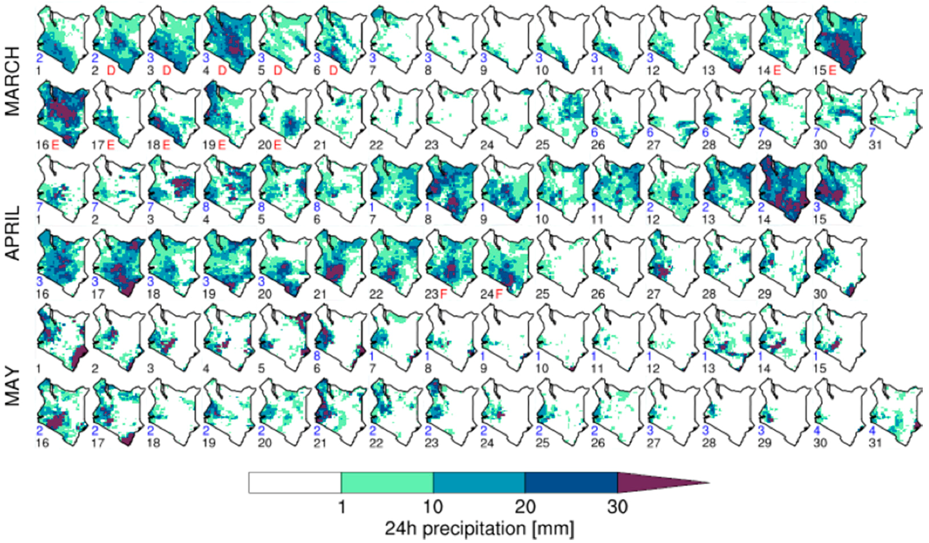
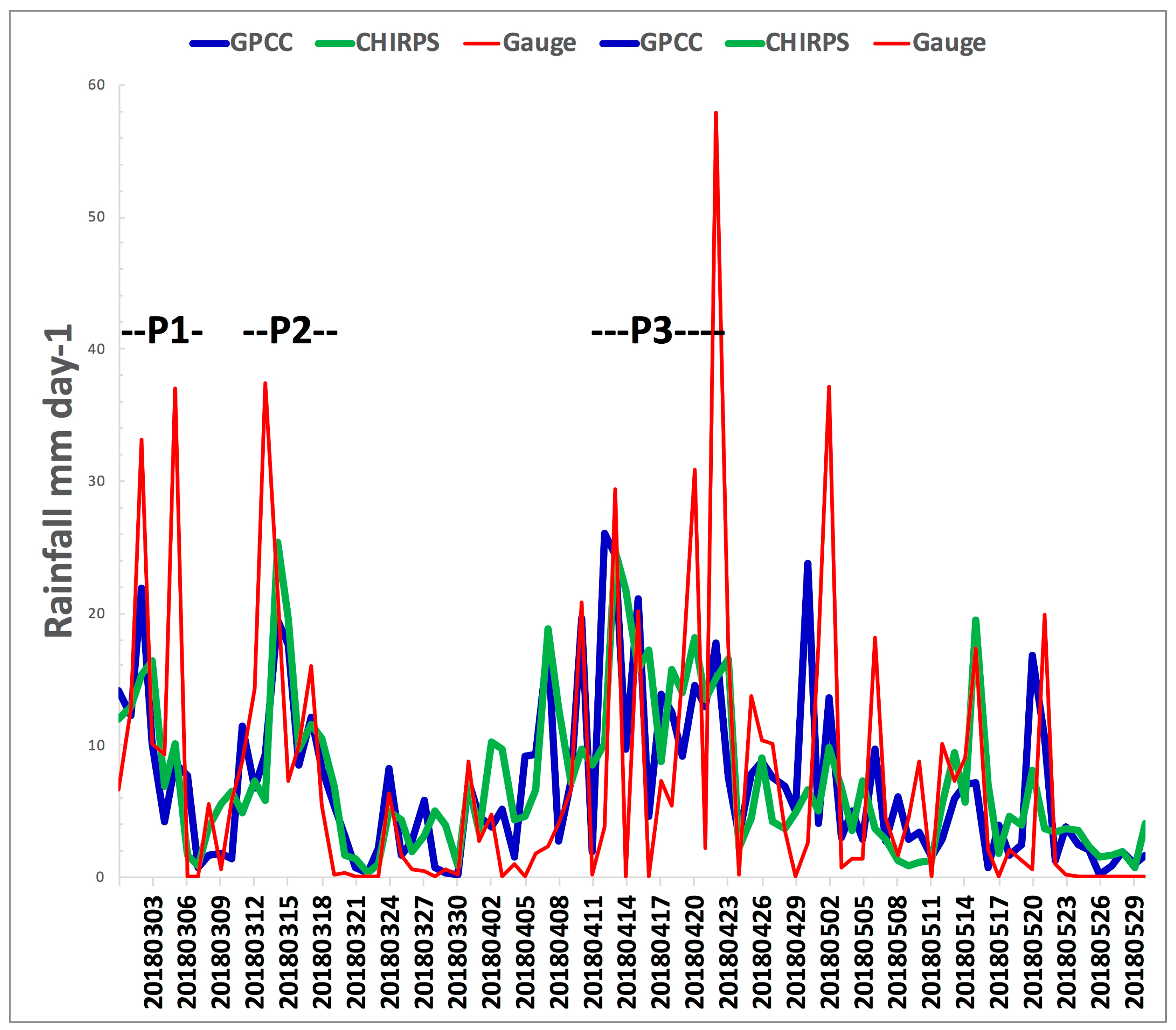
3.1. The March–April 2018 Events: Rainfall Observations

Most of East Africa experienced anomalous high rainfall during MAM 2018 (Figure 2a,b), in a zone extending from central Tanzania in the south to southern Ethiopia in the north, and from Uganda in the west to the Indian Ocean coast, and indeed extending over the western equatorial Indian Ocean to around 70° E (not shown). In absolute terms, anomalies were strongest over central and southern Kenya, including the Nairobi region. Much of Kenya experienced at least twice the normal rainfall for this wet season period and locally up to three times (not shown). Over the Kenya-core region and indeed Kenya as a whole, 2018 saw the wettest MAM season over the 119-year record of the Global Precipitation Climatology Centre (GPCC) data, and the 118 years of CenTrends data (Figure 2c). Considering all of the three-month seasons, MAM 2018 was second only to the major anomalous October–December (OND) season of 1961. Locally in Nairobi, rainfall totals at the five stations exceeded the normal amounts by two to three times in March and one to two times in April (

Table 1. Observed rainfall at five rainfall stations in Nairobi.

STATION	March Total Rainfall (mm)	% of March Long Term Mean	April Total Rainfall (mm)	% of April Long Term Mean
M.A.B.	236.8	247.3	313.6	172.9
DAGORETTI	260.3	258.2	284.8	130.5
WILSON	289.1	302.8	308.9	163.1
JKIA	216.8	291.8	229.5	168.0
KABETE	375.3	364.6	351.8	143.7

). The MAM 2018 total rainfall of 1013 mm recorded at the Kabete station was the highest on record, whilst all of the other stations recorded the third highest amounts. Overall, it is clear that a major regional scale anomaly centered over Kenya was experienced during the study period.

Analysis of the time series of daily rainfall over Kenya (Figure 3) and the Kenya-core and Nairobi area averages (Figure 4) shows that within the March–April period, the anomalous rainfall occurred primarily during three main periods of the intra-seasonal time scale. We define these as 28 February–6 March (P1), 12–19 March (P2), and 13–23 April (P3), as shown in Figure 4. In the subsequent Section 3.3 and Section 3.4, we assess the drivers of variability on these periods, and Figure 3 also shows the periods of strong activity of the two key candidate drivers of rainfall, namely the active MJO in phases 2–4 and tropical cyclones/storms in the southwest Indian Ocean (see Section 3.3). It is noteworthy that there is actually considerable variability in rainfall between the five individual stations (not shown) used in the Nairobi gauge area-average (red line in Figure 4). For example, the wettest day across Nairobi as a whole occurred on 23 April with 57 mm, but 103 mm was recorded at the Moi airbase. Such local scale variability can strongly determine the nature of associated impacts, but this is beyond our consideration in this paper.

Estimates of the return periods of within-season rainfall amounts are shown in Figure 5, with the caveat that short records of daily rainfall and inter-dataset uncertainty result in considerable uncertainty. Considering first the Kenya-core rainfall record (Figure 5a), estimated return periods for daily maximum of values are not particularly high. The March and April daily maxima might be expected to occur perhaps every one to three years within an entire year, every two to four years within the MAM season, and about every four to 14 years within the month itself. However, the five-day accumulated maximum rainfall during 2018 (which occurred during the April P3 event) was a far more unusual event, with a return period of around 10 years within the entire year, and more than 20 years in the context of the season or month. The maximum 10-day accumulated rainfall, essentially representing the P3 event, is in fact the highest in the record for both the CHIPRS and GPCC datasets, with estimated return periods of at least many decades within the year, and an even higher occurrence likelihood within the season or month. As such, during MAM 2018, the major intra-seasonal events P1–P3 are far more extreme that the daily rainfall events.

In comparison, estimated return periods for the smaller local Nairobi area are lower (Figure 5b), which probably reflects the generally higher baseline variability over smaller scales. However, the broad pattern of higher return periods for intra-seasonal five-day and 10-day maxima compared to one-day maxima is consistent with the larger Kenya-core region. Note again the effect of local scale variability, with the 23 April daily event representing a one in approximately four-year event (within the MAM season) for Nairobi as a whole (Figure 5b), but a one in >20 year-event at the Moi Air Base (not shown). Finally, considering the number of heavy rainfall days (>10 mm), March–April had more than any other year in both GPCC and CHIRPS data (not shown), which is consistent with strong intra-seasonal events. In summary, we find that the March–April season was exceptionally wet, and that this is more a reflection of exceptional rainfall at intra-seasonal timescales rather than daily rainfall. This is consistent with our analysis of the nature of the drivers of these events (Section 3.3).

3.2. Impacts of the Events

The 2018 extreme rainfall had major impacts on Kenya. Much of the country suffered from surface flooding, with 40 out of 47 counties affected. Many of Kenya’s major rivers rise in the central highlands, which experienced the most extreme rainfall (Figure 2). In total, there was an estimated 186 flood-related deaths [33,34]. The highest single death toll of 47 persons was caused by the collapse of Solai dam in Nakuru County on 9 May 2018, which was partly due to an accumulation of water volume during the preceding months of March and April, although poor construction is a possible contributor. Several other smaller dams were destroyed in other parts of the country, and many rivers overflowed their banks. The rains also triggered land and mud slides especially in central parts of the country. More broadly, there were significant numbers of people displaced by the flooding, which was estimated in total at approximately 300,000, especially in Mandera and Tana River counties, and there were around 800,000 people affected in some way [33]. The degree and duration of flood displacement was variable, and information is incomplete, but these were most severe along the lower Tana River [34,35], requiring humanitarian assistance from the government and humanitarian agencies [36,37].

The floods also submerged an estimated 21,700 acres of farmland, destroying crops within the same counties that had been affected by drought, and killed more than 19,000 livestock [33]. However, the impacts of the rains are differentiated, and these losses must be set against wider benefits to agriculture of good rains nationally. The Ministry of Agriculture anticipates a substantial increase in national maize yields this year due to the high rainfall [38], and improved pasture conditions will benefit pastoralist livelihoods in the arid and semi-arid counties that had experienced prolonged drought the previous year. Further, surface and groundwater resources will have been replenished with, for example, increased hydropower electricity generation [39].

Floods and rain damaged or rendered critical infrastructure and services inaccessible [33]. Sections of roads were cut off, paralyzing transport and preventing access to health facilities and many other services across many counties [33]. As a result, outbreak and the spread of diseases was reported [37]. In Nairobi, city severe flash flooding occurred during the three events P1–P3, temporarily paralyzing part of the transport system and greatly inconveniencing residents. The repair of the damaged roads has been estimated to cost about $187 million throughout the country and about $1.4 million dollars for about 23 roads within Nairobi [40]. In Nairobi, the rainfall caused flash flooding in the city and flooding in low-lying areas and along river courses where most of the informal settlements are located. It is likely that the flooding was more severe during the P1 event because the drainage systems had not been cleaned, but were cleared after the P1 event. Hundreds of schools were closed temporarily, affecting more than 100,000 students [33]. Overall, the impacts of the extreme rainfall and floods that were experienced were significant and widespread, although the information is partial, and may not reflect particular impacts and their severity across different locations.

An extensive relief effort was necessary during the flooding. It included an emergency appeal by the International Federation of the Red Cross for about USD $4.8 million on 1 May 2018 to assist 150,000 people. Later in May, the Kenyan government and international donors committed around USD $5 million for relief [33]. The United Nations Central Emergency Response Fund (CERF) approved an allocation of USD $5 million to support the life-saving response to people affected by floods in counties all over Kenya, from the southwest (Baringo and Kisumu) and northwest (Turkana) through central Kenya (Isiolo) to the east (Tana River, Garissa), northeast (Mandera), and southeast (Kilifi). Overall, flood relief activities extended from March until October 2018 to assist over 600,000 people [33,37]. The counties most affected by flooding according to the National Disaster Operational Center and the Kenya Red Cross Society [33] included those in the northeast (Garissa, Wajir, and Mandera), the southeast (Makueni, Kitui, and Taita-Taveta), Marsabit, Isiolo, and Samburu to the north, Tana River and Kilifi at the coast, Turkana and West-Pokot over the northwest, Kisumu to the west, and Narok over the southwest.

3.3. The Atmospheric Circulation during the Extreme Wet Periods of March–April 2018

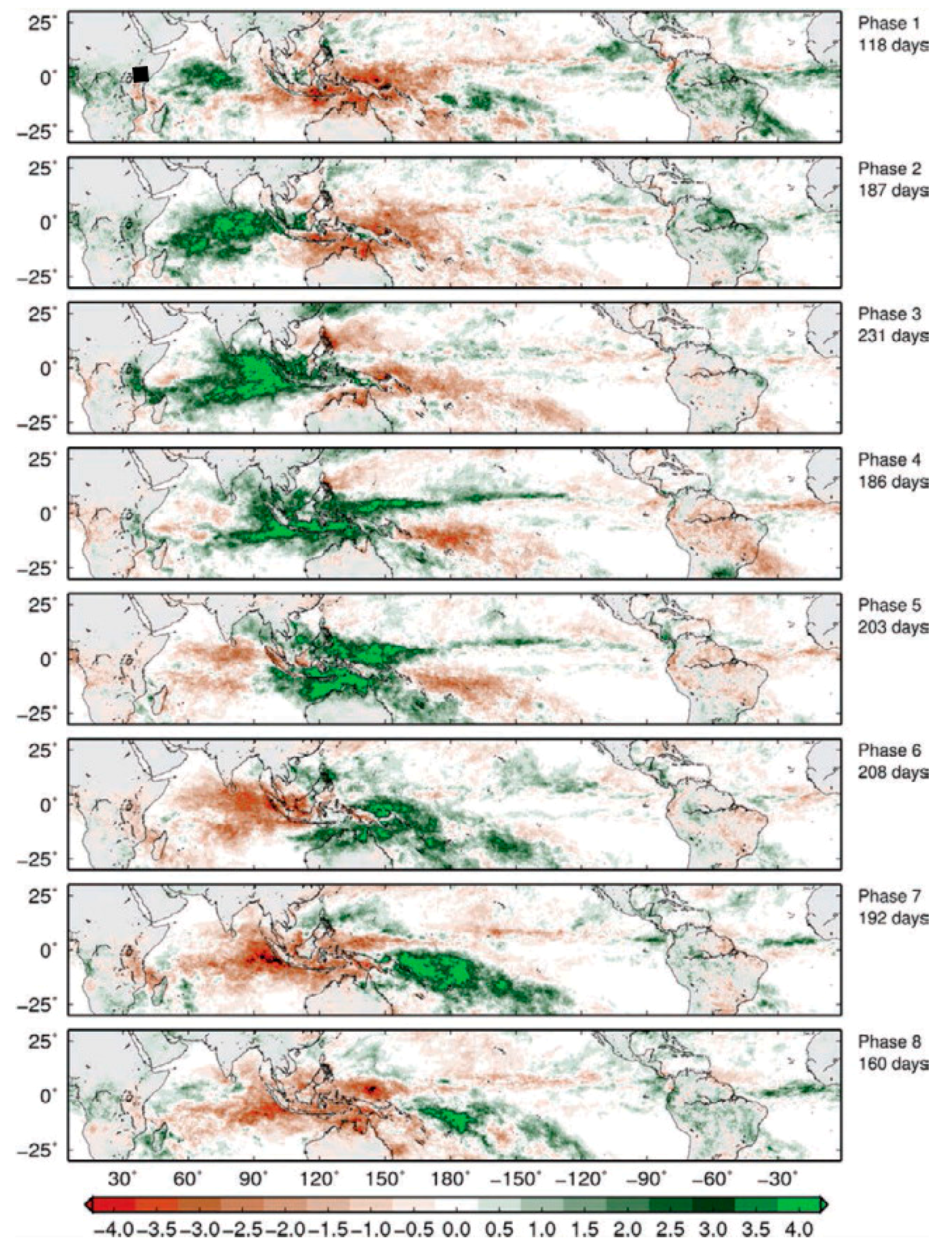
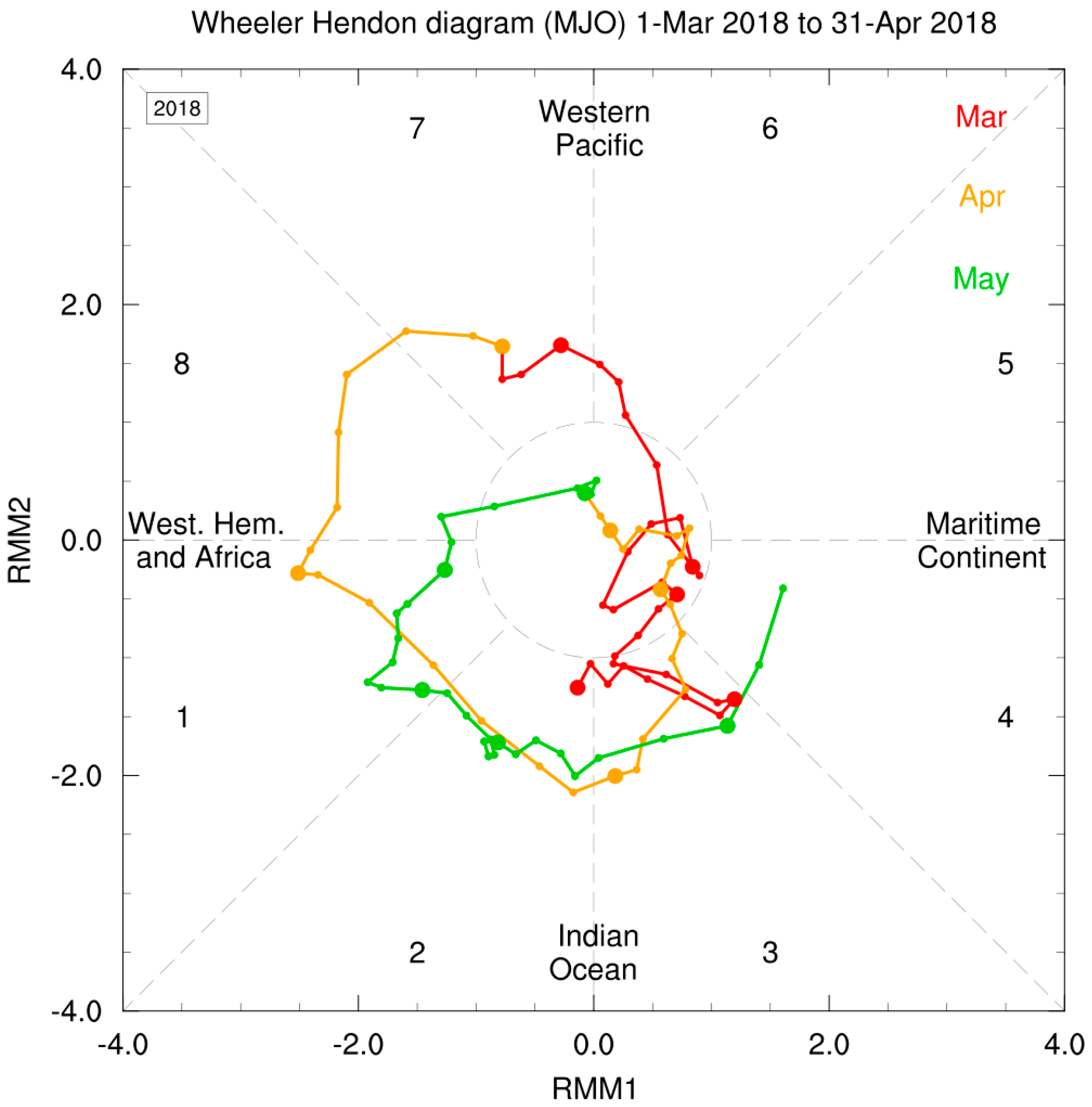
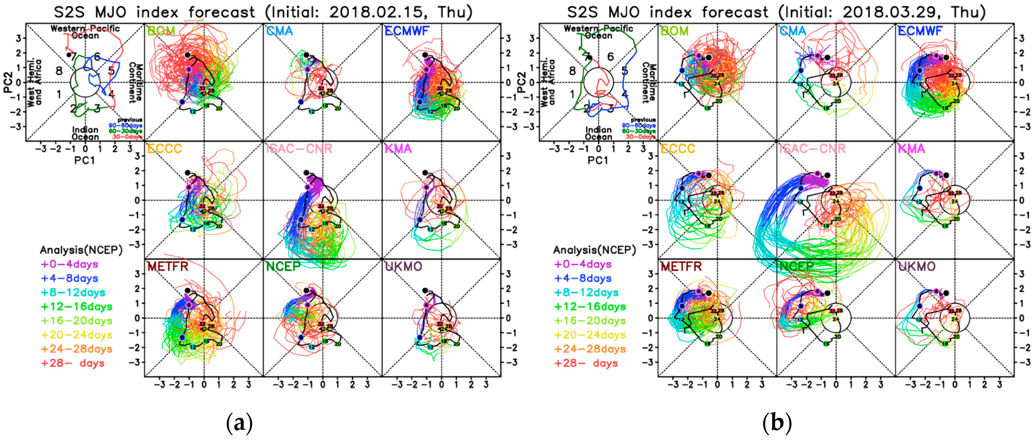
3.3.1. The MJO in Early 2018

From Figure 1 and from previous work [13], it is apparent that the MJO can lead to an anomalous enhanced rainfall over the central highlands of Kenya during MJO phases 2–4 when the main center of enhanced convection is concentrated over the western Indian Ocean. Figure 6 shows the status and evolution of the MJO during the study period. The MJO was very active in phase 3 in early March, peaking around 7–9 March. By 13 March, the MJO had become rather inactive as it transitioned into phases 4 and 5. However, there then followed a very rapid transition back to a very active phase 2 by 12 April, continuing into phase 3 during 15–20 April. Broadly, the MJO phasing and activity in March and April 2018 corresponds with the periods of enhanced and suppressed rainfall over Kenya (Figure 3). Rainfall periods P1 and P3 correspond to periods of MJO activity in phase 3, which is consistent with an analysis of the links between MJO and East Africa rainfall [14]. We note that the MJO returned to phase 2–3 during late May, but without extreme rainfall occurring over Kenya (Figure 3). We suggest that this is most likely due to seasonal changes in the large-scale circulation; notably, the intensification of the Somali jet in late May tends to advect cool, dry air with low moist static energy to East Africa from the winter hemisphere and reduces off-coast sea surface temperatures (SSTs) due to coastal upwelling, leading to conditions in which convection is suppressed [41].

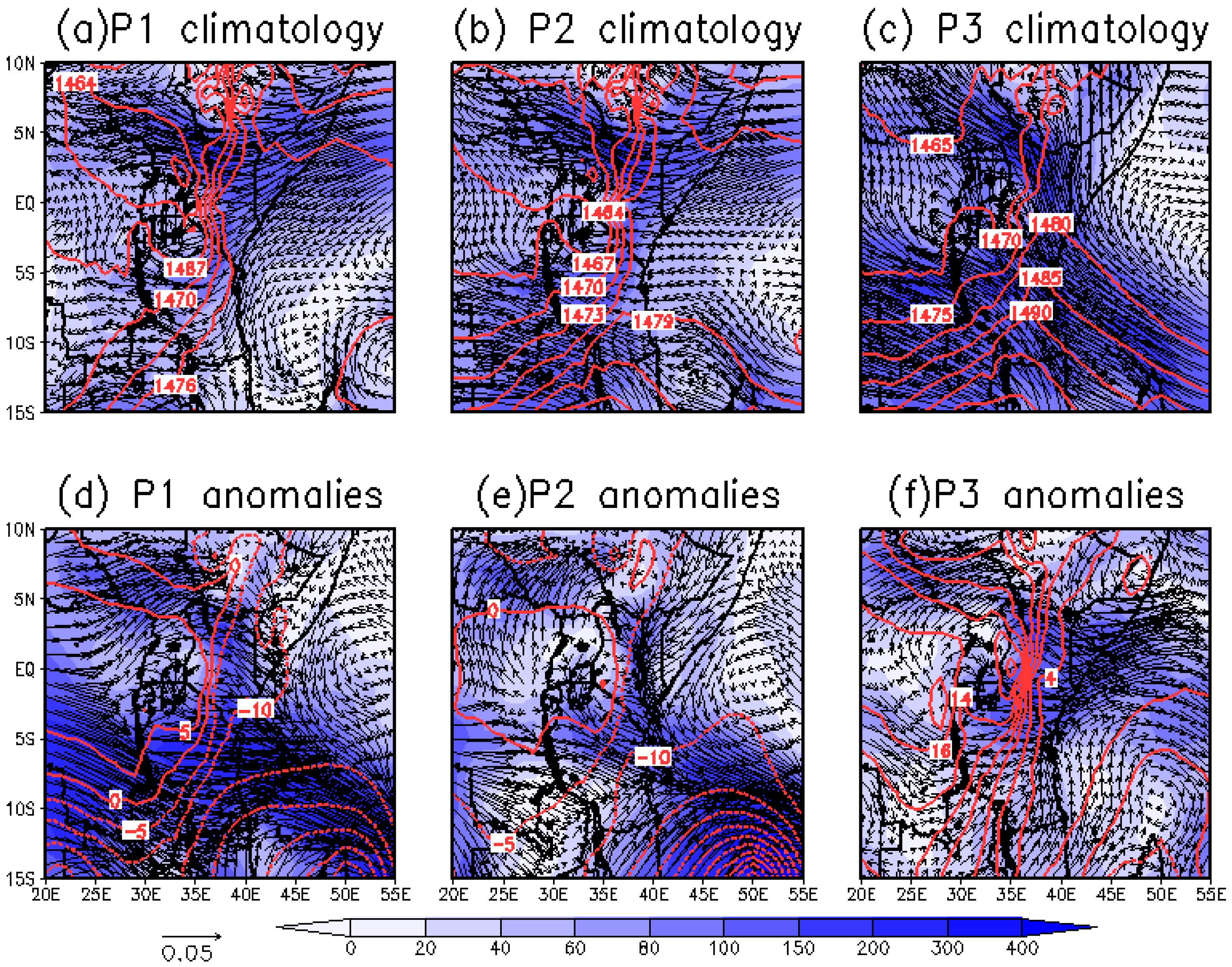
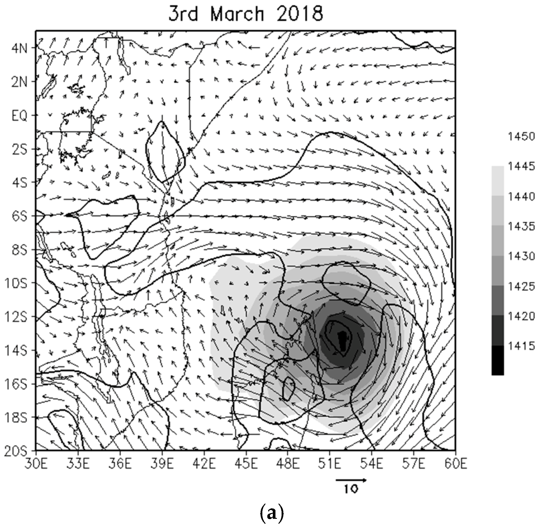
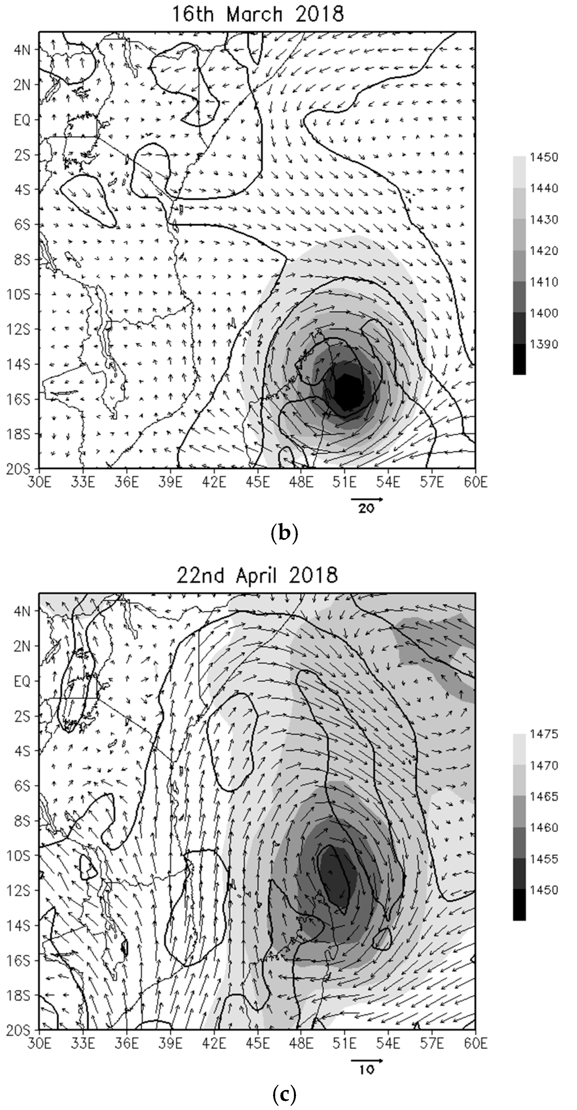
3.3.2. Regional Circulation over East Africa

Composites of the low-level circulation (Figure 7) show that all three wet periods P1–P3 are associated with strong westerly or northwesterly anomalous low-level circulation. This is broadly consistent with the circulation anomalies during active periods of MJO in phases 2–3 identified in composites of Pohl and Camberlin [13] and Hogan et al. [17]. The composite circulation anomalies also show a strong influence of tropical cyclones/storms in the southwest Indian Ocean in periods P1, P2, and P3 when tropical cyclone Dumazile and tropical storms Eliakim and Fakir, respectively tracked southward close to the east coast of Madagascar. The circulation on individual days within the P1–P3 event periods (Figure 8) shows these cyclone systems more clearly, suggesting that that these three tropical cyclones/storms contributed to the low-level westerly wind anomalies across the equatorial western Indian Ocean. As such, we infer that the combined effects of active MJO in phase 3 and the presence of deep tropical low pressure centers off northwest Madagascar led to strongly anomalous westerly low-level circulation. Previous work has linked the MJO activity in phases 2–4 itself to enhanced tropical cyclone formation in the southwest Indian Ocean [42].

3.4. Predictability of the Extreme Wet Events of March–April 2018

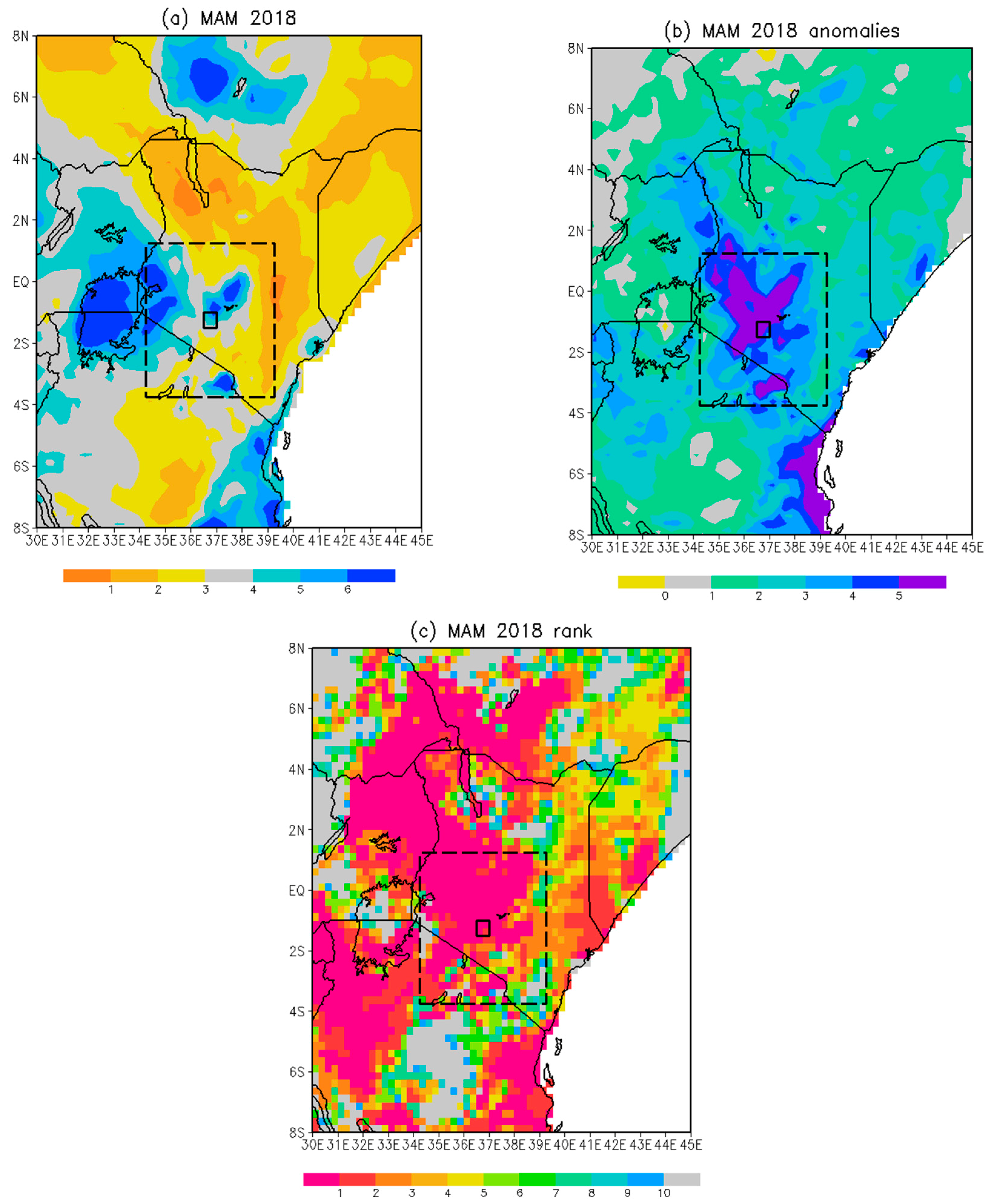
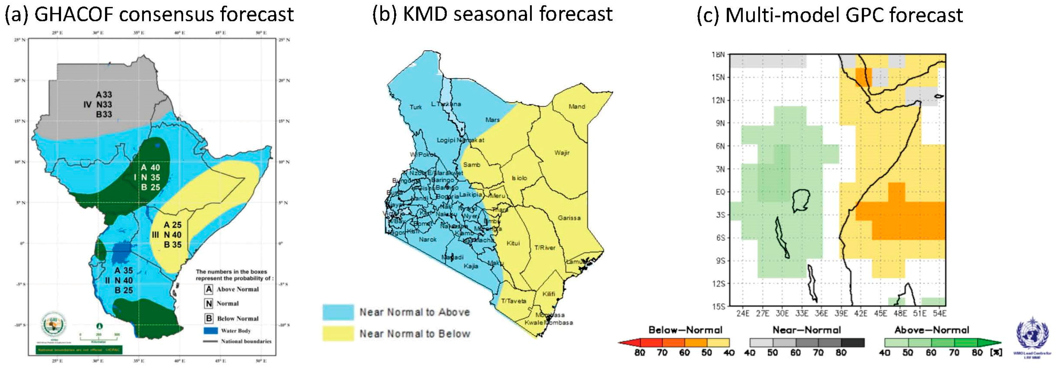
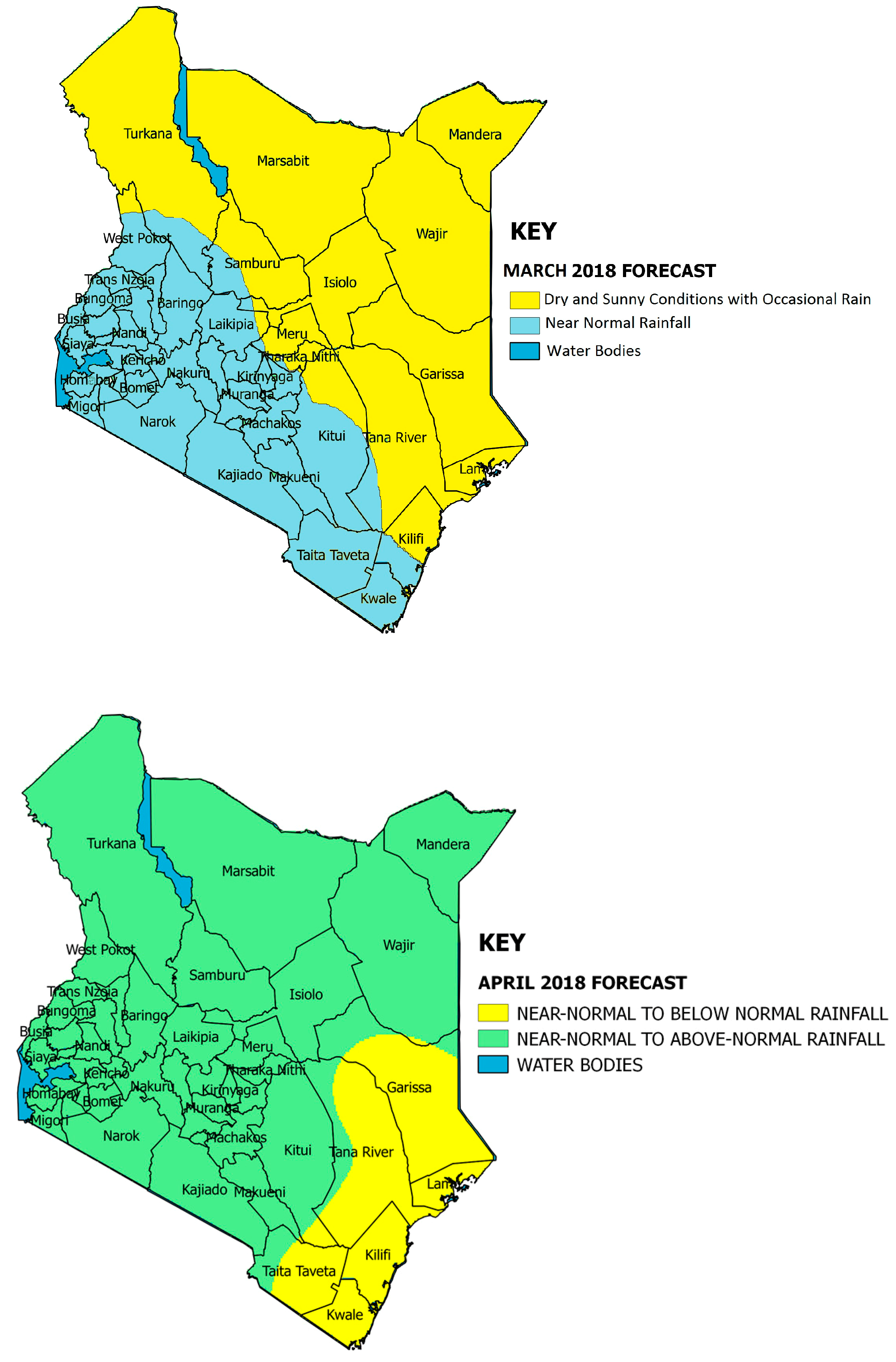
3.4.1. Seasonal Forecasts for MAM 2018

The GHACOF seasonal consensus outlook product issued in mid-February 2018 (Figure 9a) has no clear indication of wetter than normal conditions for the MAM season over Kenya or indeed anywhere in East Africa. This is also the case for the KMD national forecast (Figure 9b). The GHACOF and KMD forecasts partly reflect the 13-model multi-model WMO GPCs forecasts (Figure 9c), though only about half the models would have been available at the time the consensus was generated (5–10 February). The GPC multi-model forecast indicated weakly enhanced probability of the above normal category in the west of the region (green shading) and weakly enhanced probability of below normal in the east and northeast. However, accompanying hindcast skill in the former region is low, although higher in the latter (not shown).

We next examine forecast output from the ECMWF (S5) and UK Met Office (GloSea5) GPCs in more detail (Figure 10a–h) and focus on the rainfall upper quintile, which is likely to be more directly indicative of heavy rainfall within the season. The forecasts initialized at the start of February from ECMWF S5 had no clear indication of wetter than normal conditions (Figure 10a), whilst the UK Met Office GloSea5 product had increased probabilities of a wet event over the west of the GHA, but not over most of Kenya (Figure 10b). However, those forecasts issued at the start of March (Figure 10c,d (i.e., at a zero-lead for the season)) indicated strong wet rainfall anomalies. That there is only an indication of enhanced risk of the observed high rainfall in the forecasts initialized at the start of March, and not in those initialized at the start of February is unsurprising given the analysis of forecast skill at these two lead times (Figure 10d–h). This verification analysis across the hindcast 1993–2018 (Figure 10d,h) reveals much higher ensemble mean correlation with observations for the March initialized forecasts, and very low skill for the February initialized hindcast. Note that ECMWF S5 forecasts are initialized with data from an ensemble on the first day of the month, whilst GloSea5 ensemble members are initialized from days centered on the first day, including up to 10 days into the month. So, the results are not directly comparable, and GloSea5 has a slight ‘advantage’ in that, at this zero-lead range, it has access to initial conditions in the first 10 days of the target season.

The March 2018 case is consistent with the understanding that a long lead time indication of anomalous rains over Kenya for MAM does not have a strong basis, given the lack of slowly evolving drivers and subsequent low seasonal forecast skill. However, the analysis indicates that skill exists for a ‘late view of MAM’ (i.e., with only zero-month lead-time) and in 2018, a forecast for an anomalously wet MAM 2018 was made on 1st March by the S5 and Glosea5 models. This suggests a potentially useful role for a last-minute updated outlook of the season issued at the start of the season. In a seamless way, this may bridge the gap between the seasonal long lead outlooks and the potential skill from the sub-seasonal forecast products, where skill for individual extreme rainfall periods within the season may be possible due to the predictable signal arising from the link between East African rainfall and the MJO. These sub-seasonal outlooks are considered below, focusing on the heavy rainfall periods observed in the first half of March and mid-April.

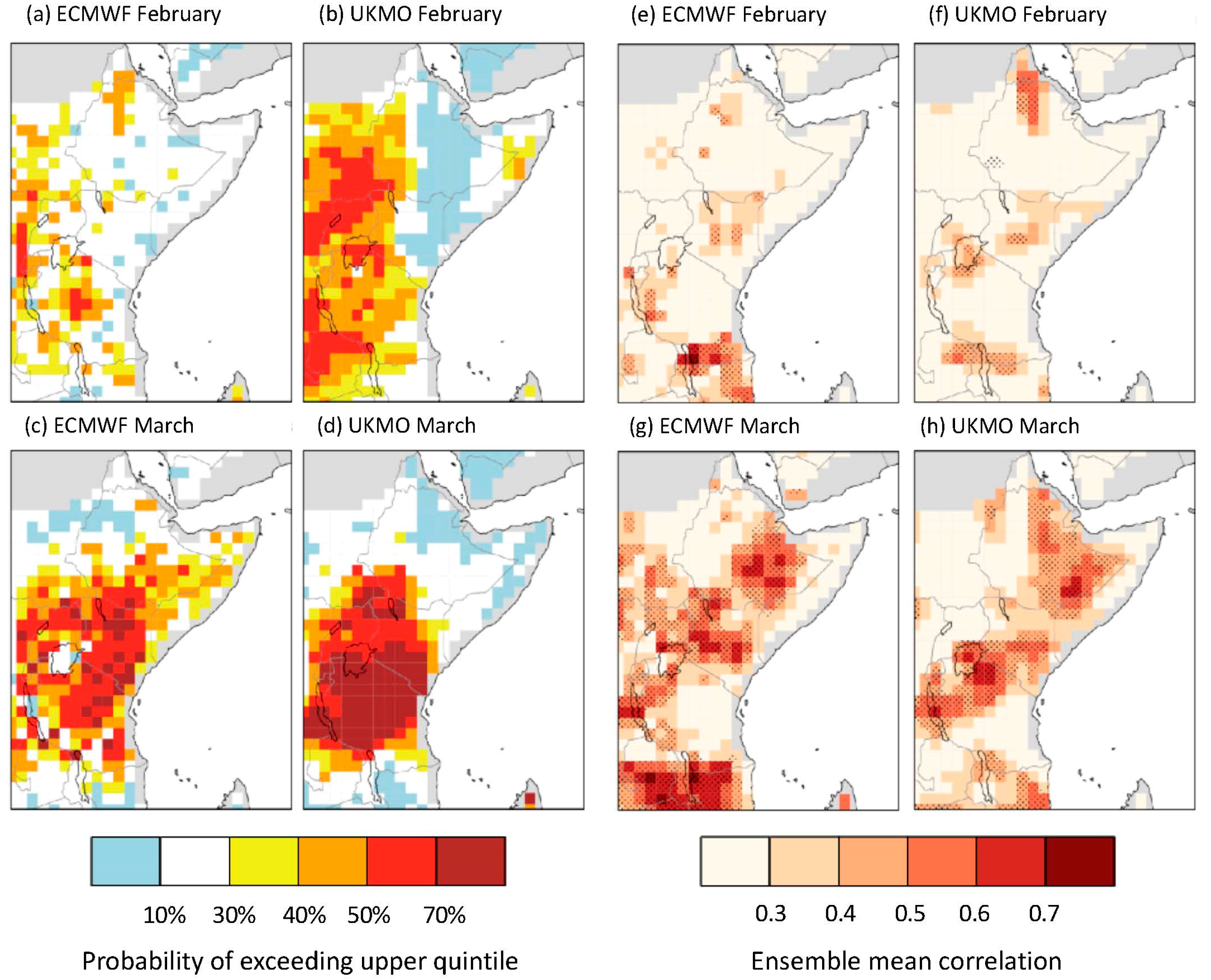
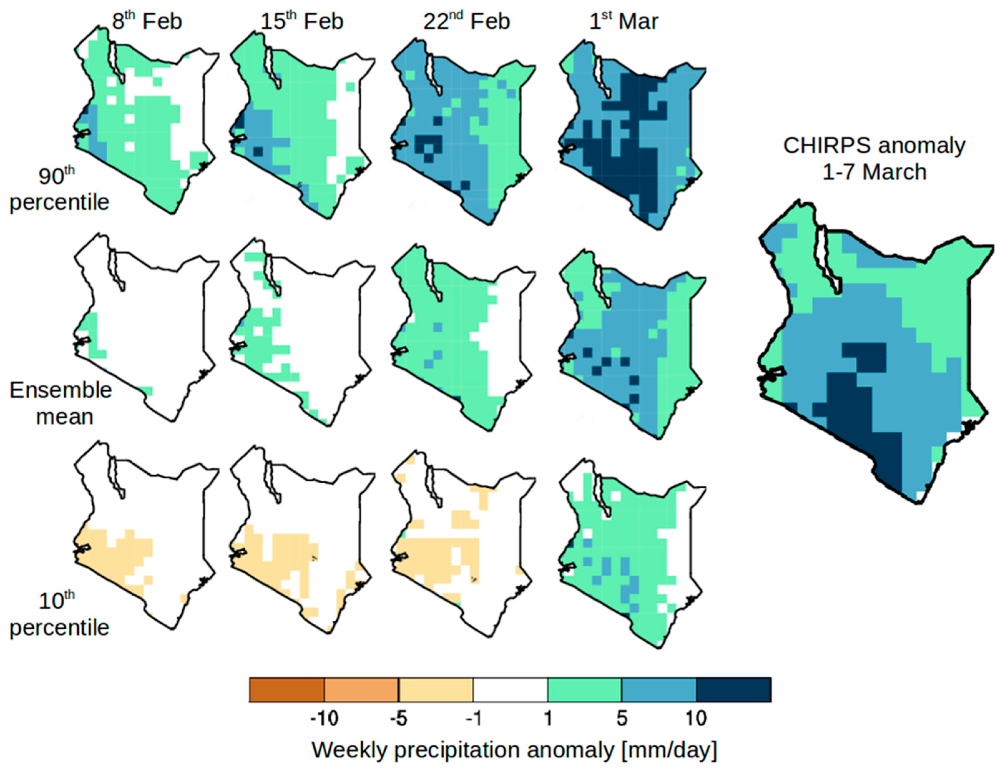
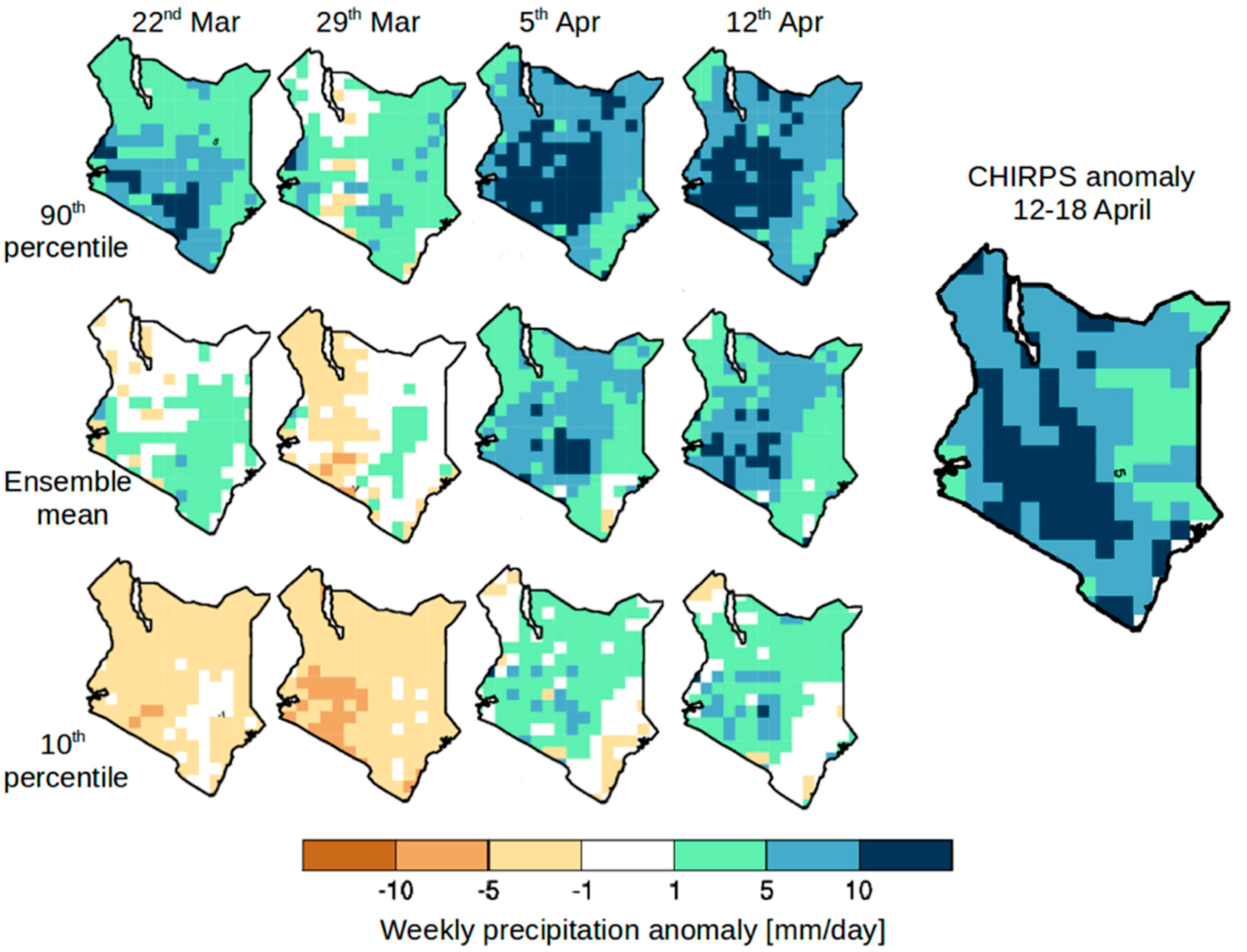
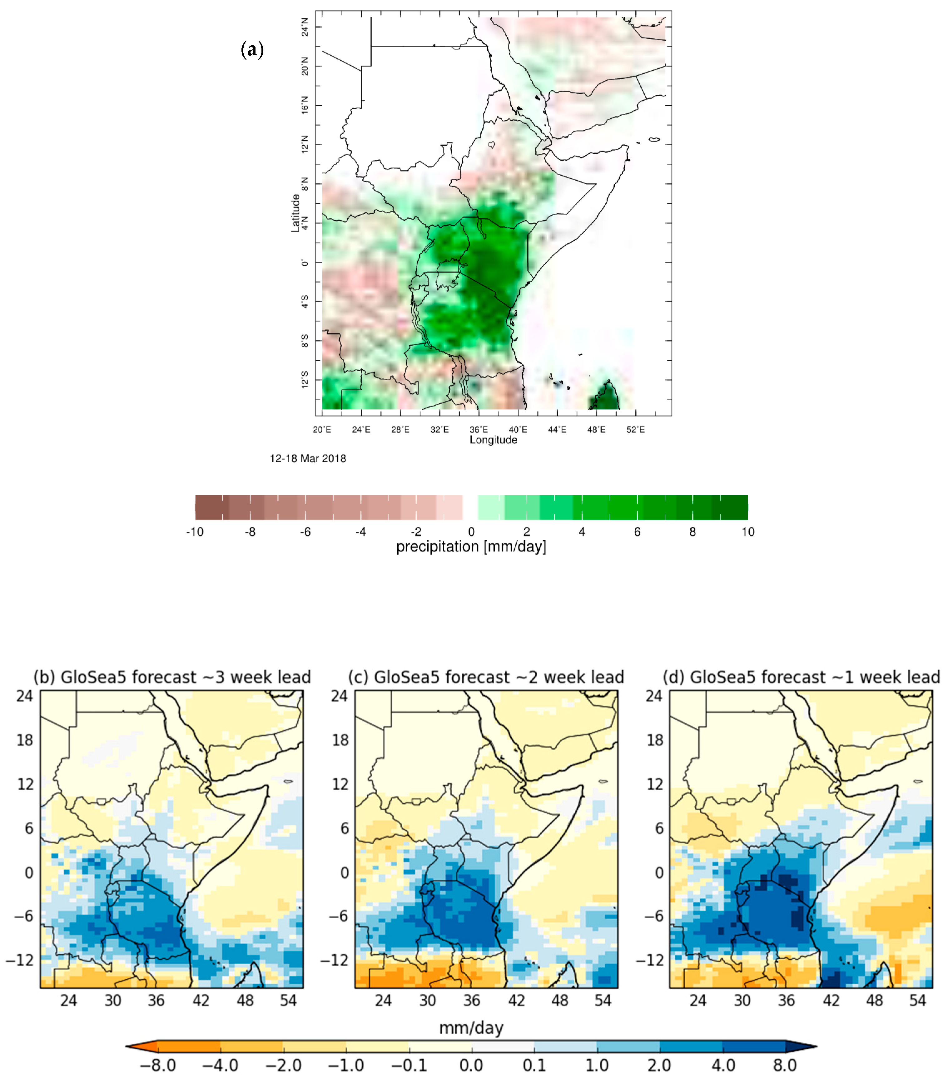
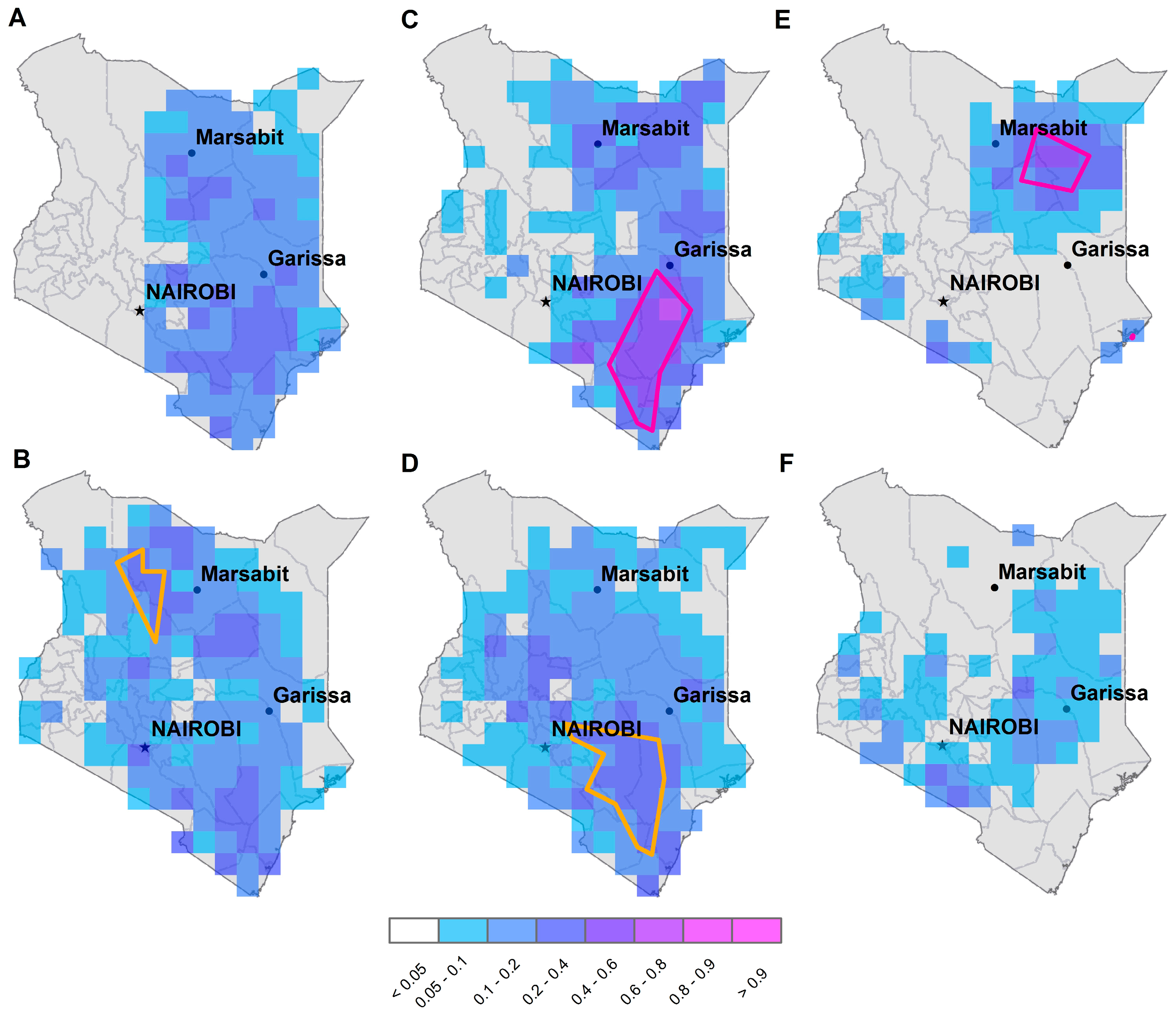
3.4.2. Extended Range Sub-Seasonal Forecasts

First, we consider the predictability of the MJO in models (Figure 11); then, we consider the specific rainfall forecasts over the region for the rainfall events P1–P3 (Figure 12, Figure 13 and Figure 14). For MJO forecasts from the S2S hindcast database (Figure 11), two start dates are shown: 15 February and 29 March, each two to three weeks in advance of the rainfall events occurring at the start of March (P1) and in mid-April (P3), respectively. Consider first the 15 February initialized forecast. At this point, the MJO was active in the Western Pacific in phase 7, before moving relatively quickly around into phases 1, 2, and finally phase 3 in early March (see also the observed MJO in Figure 6). As noted in Section 3.3.1 and Figure 3, the MJO in phase 2 and 3 at the start of March was concurrent with the heavy rainfall period P1 over Kenya. Model forecasts for this MJO track show some variability; however, most show a clear indication of the ensemble moving into zones 2–3, with a relatively high density of the ensemble at around 16 days (i.e., the start of March 2018) indicating an active MJO in this region. The ECMWF S5 and UK Met Office Glosea5 (referred to as ‘UKMO’ in the figure) systems show particularly a high ensemble density, indicating relatively high confidence in this MJO track. Other start dates for this period are shown in the Supplementary Material (Figure S1); for the forecast issued one week earlier on 8 February, there is a high uncertainty in most systems, with little indication of an active MJO in the zone 2–3 period in early March. For the 22 February start date, the forecast ensemble spread tightens for the early March period, whilst for the 1 March forecast, models vary in their ability to capture the curvature back into zone 3 on 8 March. Particularly, the UKMO and KMA (a version of GloSea5) capture this, whilst the BOM model forecasts a continued progression of active MJO into zone 4.

Considering the MJO and the P3 rainfall event in mid-April 2018, a similar MJO track occurred in this period; starting in phase 7 and moving quickly eastwards to end up in phase 2–3 around day 16 (roughly mid-April). The forecasts initialized on 29 March (right panel of Figure 11) provided a two to three-week lead forecast for this event. Again, some models captured this pattern: most notably the ECMWF and UKMO, which gave a clear ensemble consensus of the eastward propagation. Alternative start dates in the Supplementary Material (Figure S2) show a similar picture: the earlier initialization of 22 March shows little indication of the eastward track, whilst the 5 and 12 April initializations shows clear model and member consensus on the movement into MJO zone 2–3.

These results are consistent with the verification of MJO skill in the S2S database by Vitart et al. [26], which show that the ECMWF and UKMO models consistently have higher bivariate correlation for the MJO than the other models, with MJO correlation remaining above 0.6 until several weeks ahead. Other models have lower correlation, with some limited to one week of skillful MJO prediction. Given the key East Africa link with the MJO, this suggests that sub-seasonal forecast models with a better ability to predict MJO at long lead times have more potential for use in early warnings, although the forecast skill for precipitation over east Africa will ultimately depend on the model representation of MJO teleconnections.

To illustrate the potential to increase the lead time of warnings beyond the one-week range, we showcase study results for rainfall forecasts from the two sub-seasonal systems with the highest skill for MJO prediction, ECMWF and GloSea5. Both systems show encouraging predictability for all three episodes, P1, P2, and P3. Here, for brevity, we show Kenya-specific results for P1 and P2 from ECMWF Figure 12 and Figure 13, and for P3, we illustrate prediction on the larger scale context using GloSea5 (Figure 14).

Figure 12 and Figure 13 present weekly ECMWF rainfall anomaly forecasts for leads of one to four weeks ahead, which are expressed as the ensemble mean as well as the 10th and 90th percentile to indicate the spread of the ensemble. For the early March P1 period, little signal is seen in the ensemble mean at four weeks lead, and this is only slightly increased at three weeks lead (as indicated in the first and second columns, respectively). By the lead time of two weeks ahead (as shown in the third column), the ensemble mean forecast shifts toward wet conditions for most of the country, with an increased probability of significant rainfall (with over half the country >five mm/day across the week). For the one-week lead forecast (the fourth column), the ensemble mean shifts significantly, and the probability of an extreme weekly anomaly of over 10 mm/day increases significantly, and the ensemble suggests little probability of a dry week, with even the 10th percentile of the forecast indicating over five mm/day in places.

For the mid-April P3 period (Figure 13), there is a strong indication of a significantly wet week in the ensemble mean at one and two weeks ahead, with the 90th percentile of the ensemble indicating the possibility of extremely wet weeks, and the 10th percentile suggesting that a dry week is quite unlikely. There is also a strong signal even at the week four forecast, issued on 22 March. This slightly drops off for the week three forecast, although a consistently wet signal remains, albeit weak in the ensemble mean.

These results are broadly consistent with the lead times for forecasting the MJO itself, suggesting that the rainfall events (almost seven-day averages) were captured reasonably well in the ECMWF forecast model with a roughly two-week lead time. The consistency also gives some suggestion of a physical connection between MJO activity and the resulting rainfall anomalies over Kenya. Ensemble mean forecasts from GloSea5 for the 12–18 March period within the P2 period are shown in Figure 14, and illustrate predictability on the larger East Africa scale. The area with positive rainfall anomalies covered much of Kenya and the northeast as well as central Tanzania, with the largest anomalies over northeast Tanzania (Figure 14a). The broad spatial characteristics of the observed anomalies are signaled in the GloSea5 predictions at leads of up to three weeks (Figure 14b,c). The predicted anomaly magnitudes are less than observed (peaks of approximately six mm/day relative to nearly 14 mm/day), but this is expected from the ensemble-averaging process. At week three (Figure 14b) and week 2 (Figure 14c), the main area of rainfall is predicted slightly too far south. Nevertheless, there is very good indication of a heavy rain event, with the largest rainfall anomalies impacting mainly eastern Tanzania and southern central Kenya from week two onwards.

The KMD monthly forecast for March 2018 (Figure 15) issued on 2nd March during the P1 period showed no indication of an exceptionally wet month. It indicated the likelihood of near normal rainfall over the southern, central and western parts of the country and dry conditions over the northern and eastern parts. By this time, the role of both the MJO and the tropical cyclone (Dumazile) in enhancing the rainfall was apparent but the likelihood of recurrence of a similar scenario within the month was not predicted. The April forecast (Figure 15) indicated likely normal to above normal precipitation over most parts of the country with the exception of a few counties in the coastal region and over the Southeastern parts. The evidence presented earlier in this section suggests that, at least for the MAM season, a strategy of placing more weight on dynamically-based one-month forecasts relative to statistical forecasts may increase the accuracy of issued one-month outlooks.

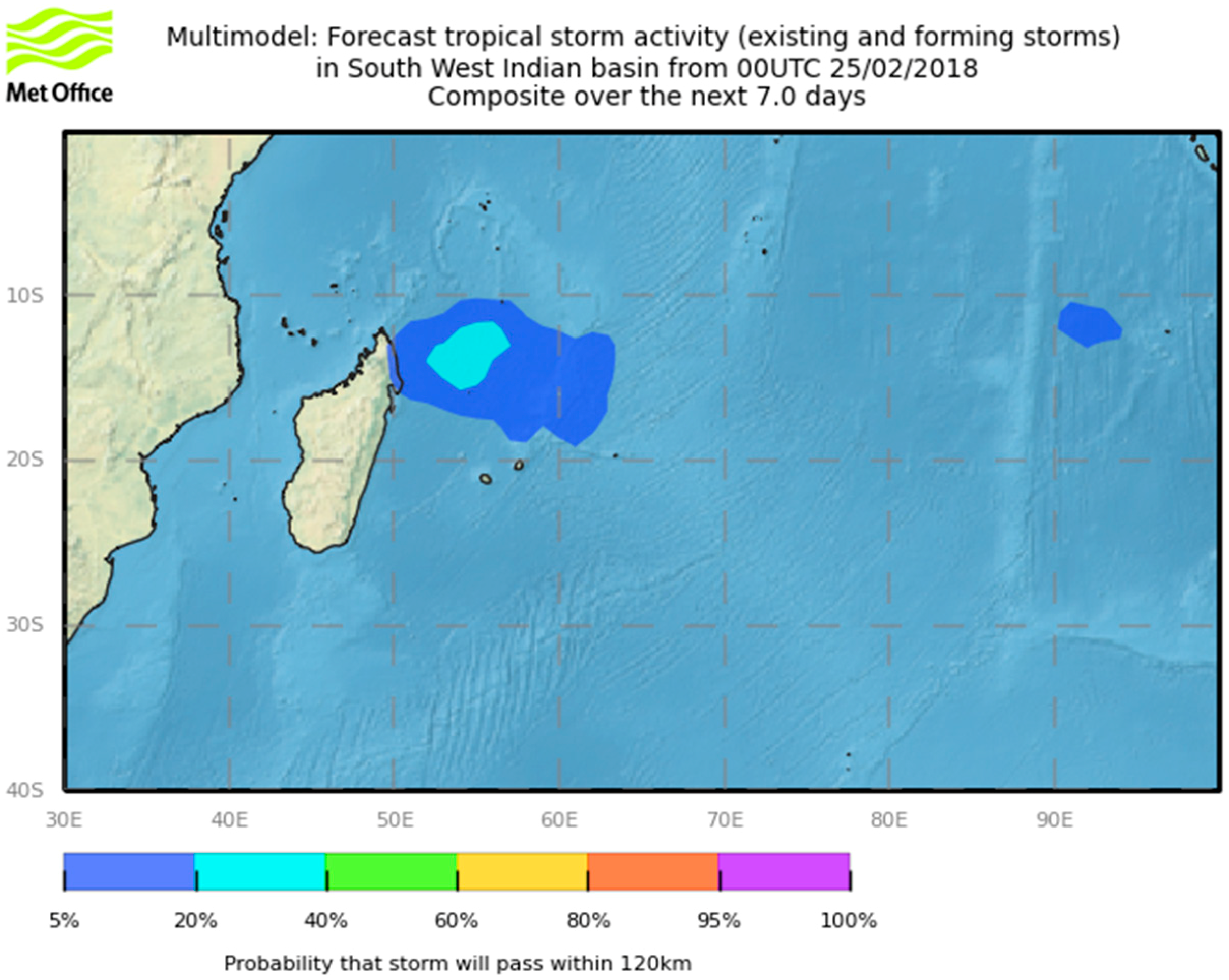
3.4.3. Short-Term Weather Forecast Timescales

(a) Performance of the GHM in March–April 2018

A qualitative assessment of products from the Met Office GHM (see Section 2.2.3) indicates that, broadly speaking, the forecast probabilities of extreme rainfall even out to a 6-day lead-time, align fairly well with observed rainfall over the March-April period, both in terms of the day-to-day variability and the spatial structure, illustrated here with three examples (Figure 16). The GHM indicated enhanced probability of high-impact rainfall for keys days in the P1 and P2 periods (Figure 16a–d), and the spatial distributions (Figure 3) at the broad scales across the country, although not at scales smaller than that approximately equivalent to counties within Kenya.

Specifically, the GHM forecast for 4 March with a six-day lead indicated forecast probabilities of between 0.2–0.4 across central Kenya. Similarly, the six-day lead GHM forecast for 16 March (Figure 16d) provided a good signal of extreme rainfall (probabilities between 0.2–0.4) across the southeastern areas of the country. However, notably, although the sub-seasonal lead-time forecast was good for the P3 period as a whole (Section 3.4.2, Figure 14), the daily distribution was less well represented. For the peak rainfall day of 14 April, the strongest signal for enhanced extreme rainfall risk at a three-day lead is located over northeast Kenya (Figure 16e), rather than southern and western Kenya, as observed (Figure 3).

These results demonstrate the capability of current global short-term ensemble weather prediction systems to highlight the risk of extreme rainfall in the region at lead times of up to a week ahead, which provided a clear signal for forecasters. This risk is reflected in the rainfall advisories issued for the P1 and P2 periods (Section 3.5), which note an enhanced risk at the scale of specific counties within Kenya. Nevertheless, the limitations in the forecast spatial accuracy must not be understated, and a more comprehensive analysis of forecast skill should be undertaken to assist forecasters with the appropriate level of precision provided in advisories. Difficulties in the model representation of convective organization continue to limit predictability at smaller scales. Higher model resolution is likely to be the way forward, and a comprehensive analysis of the Met Office’s East Africa model running at a convection-permitting grid resolution of four kilometers should be undertaken. Convective-permitting ensemble forecasts with the associated post-processing are available in only a handful regions around the world, and further work is required to assess forecast skill from these systems over our study region.

(b) Forecasts of tropical cyclone activity

Analysis of the forecasts for the three tropical cyclones/storms Dumazile, Eliakim, and Fakir (Dumazile shown in Figure 17, compare to Figure 3) suggest that for each of these three storms, the global ensemble prediction systems highlighted an increased probability of tropical storm formation roughly one week ahead of genesis; earlier forecasts provided little or no indication of tropical cyclone occurrence near Madagascar. This indicates useful predictability for these events, although the degree of consistence in the association of tropical cyclones near Madagascar and anomalous rainfall over Kenya and wider East Africa remains to be determined, and is likely dependent on the actual location and track of a given storm.

To summarise this Section 3.4 on predictability, our analysis of operational forecasts and hindcast verification where available shows that the extreme March–April 2018 rainfall was not predicted, nor likely to be predictable with a long lead of more than a few weeks. This is to be expected, given the weak coherence of the MAM season and lack of large-scale drivers, and hence weak predictability. Zero-lead seasonal and sub-seasonal ECMWF forecasts with two-week lead times identified the specific intra-seasonal events P1–P3 and the likely MJO drivers. This analysis suggests the strong influence of MJO and synoptic scale tropical storm/cyclone events in driving the events. There is some evidence in the short term weather forecasts of reasonable prediction out to a one-week lead time, which resulted in KMD advisories highlighting the enhanced risk of heavy rain for the P1 and P2 events in March, but not for the P3 event in April.

3.5. Flood Warnings and Related Response Actions in 2018

KMD advisories issued to the general public and risk management agencies reflect the signals in the forecasting system that were described in detail above. Specifically, (i) The long-lead seasonal forecasts showed no indication of enhanced seasonal or within-season rainfall or extremes nor resulting flood risk. (ii) Regarding the sub-seasonal lead times, the monthly forecast for March (Figure 15) showed no indication of enhanced rainfall. In contrast, the April monthly forecast indicated that most parts of the country would experience enhanced rainfall, and the experience during March may have raised the credibility of the forecast. (iii) Regarding short-term weather advisories, the KMD five-day and seven-day forecasts are informed by ECMWF, NCEP-GEFS, in-house WRF forecasts, and the GHM. During the periods immediately preceding the P1 and P2 rainfall events in late February and around 9 March, the key forecasted signals of active MJO phase 2, the existence of tropical cyclones Dumazile and Eliakim, and the resulting enhanced risk of heavy rainfall were noted. Accordingly, heavy rain advisories were issued for two periods: 1–3 March (Figure 18) and 12–16 March, with lead times of two to four days (issued 27 February) and three to six days, respectively. These periods do fall within the P1 and P2 events, and the areas that were identified as being at risk (the western and Rift Valley counties) were broadly coincident with the actual rainfall anomalies (Figure 3).

The heavy rain advisories were disseminated quickly through various channels (social media, radio, and print media). Daily updates gave further indications of the timing of the rainfall. The forecasts were broadly accurate, but the short lead time limited the extent of possible advanced preparedness actions. In addition, the message that the P1 event did not represent the LR onset resulted in a lack of preparations by many farmers for seasonal planting. The successful forecast of the P1 episode and the direct experience of the impacts raised the credibility of the KMD and attention on the subsequent forecasts, such that there was a higher level of alert and sensitivity to the warnings for the P2 period. However, there is some indication that the agricultural sector in particular had not yet fully prepared for planting when the P2 event occurred. Specifically, for Nairobi city, weekly forecasts for the county were downscaled from the national forecasts and issued one day after the national forecasts. Advisories were sent immediately via emails to county government heads for disaster risk, infrastructure, roads and transport, agriculture, and to non-governmental organizations (NGOs), and community-based organizations, especially those in informal settlements and media organizations. Regarding the P3 period, although the weekly forecast issued on 9 April for the period between 10–16 April (part of the P3) and the forecast issued on 16 April for the period between 17–23 April, indicated that heavy rainfall would occur over many parts of the country, no heavy rain advisory was issued.

Whilst we are able to document the specific advisories that were issued, it is not possible at this stage to fully document the resulting actions. However, some examples are provided below.

(i)

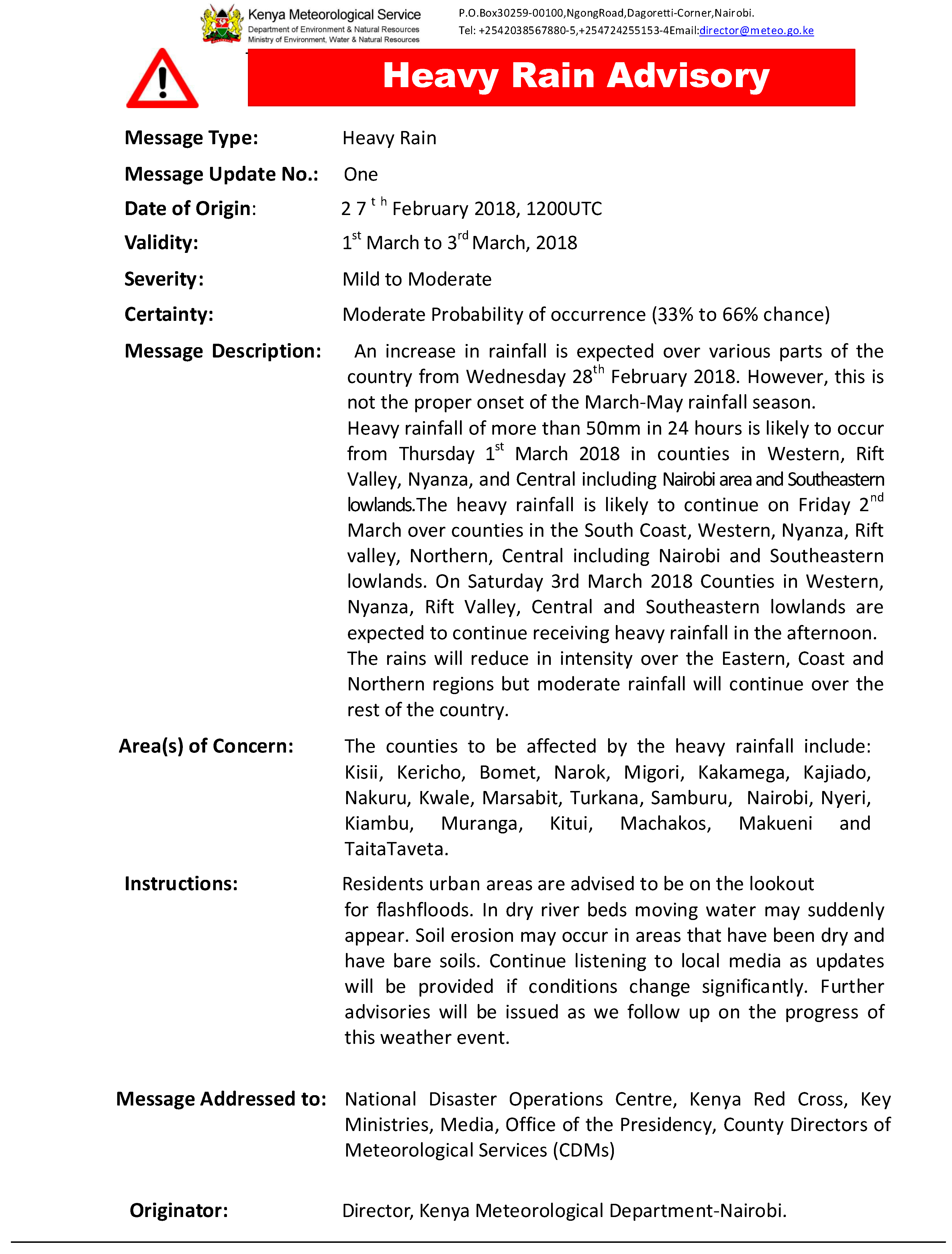
The Kenya Red Cross Society (KRCS) used the KMD five-day and seven-day forecasts and advisories to issue warning alerts for rain and flood (e.g., the alerts for rain/flood issued 17–18 March). These were based on an update to the 12–16 March KMD advisory issued on 15 March (during P2 event), which was issued via mobile phone text messaging, targeting almost 10 million people in the western Kenya, Nyanza, Nairobi, Coast, Rift Valley, and Mt. Kenya areas. During the season, the KMD five-day and seven-day forecasts were presented at the flood meetings held at KRCS headquarters (HQ) in Nairobi, to coordinate action in the flood prone regions, notably the Tana River floodplain. The KRCS Disaster Management Operations (DM Ops) team expressed a demand for longer lead forecasts (i.e., about two weeks to a month). In the absence of timely products with those lead times from the KMD, intra-seasonal outlooks from international portals were analyzed. This information was used by the KRCS to infer likely future flood impacts and response needs.

(ii)

Within Nairobi, there is some indication that the flooding during the P1 event and subsequent KMD advisories stimulated a response by agencies to mitigate flooding. Some actions were taken by mid-March, including: Nairobi county budgeting for casual staff and equipment to respond to flooding; and the rapid clearing of drainage and sewerage systems by the county government and the Nairobi City Water and Sewerage Company around the beginning of April, which may have successfully mitigated flooding during the P3 event.

4. Discussion and Conclusions

In summary, we have analyzed the drivers, predictability, and flood-related impacts of the 2018 MAM LR season over Kenya, which was one of the wettest on record. The exceptionally high monthly rainfall totals in March and April resulted from persistent heavy rain events, rather than from extreme daily rainfall. Three unusually intense intra-seasonal rainfall events were particularly notable, with return periods estimated to be up about six to 20+ years, depending on the time period considered. These events resulted in extensive flooding with over 140 deaths, significant loss of livelihoods, the displacement of people, major disruption of essential services, and damage to infrastructure. The rainfall events appear to be associated with the combined effects of active Madden–Julian Oscillation (MJO) in phases 2–4, and at shorter timescales, tropical cyclone events in the southwest Indian Ocean. These combine to drive an anomalous westerly low-level circulation over Kenya and the surrounding region, which likely led to moisture convergence and enhanced convection.

We analyzed the predictability of these specific events and equivalents in the historical model hindcasts, and noted the following. (i) The absence of any strong indication of an enhanced likelihood of heavy rain over Kenya in seasonal forecast products is not unexpected, given the low levels of forecast skill for the MAM season at lead times one month ahead and longer. (ii) However, at shorter lead times of a few weeks, the zero-month lead seasonal and the sub-seasonal extended range forecasts provided a clear signal of likely enhanced rainfall, which is likely associated with the model skill in MJO prediction. (iii) Short lead weather forecasts from multiple models also highlighted enhanced risk, and provided an important indication of extreme rainfall risk in the wider region, although forecasting the details of the exact location, timing, and rainfall amount remains challenging, even in the short range. Although we have not shown the verification statistics of rainfall forecasts specifically for Kenya, earlier results at the global scale suggest that adopting a multi-model approach is generally beneficial [32].

Our findings have some important implications for operational forecasting, early warning, and flood risk preparedness planning in Kenya and potentially adjacent countries in the East African region. Regarding forecasting, our analysis indicates that during the LR, emphasis should be placed on the sub-seasonal and short-term forecasting lead times, which show potentially useful skill (whilst recognizing the challenges of forecasting at small-scale precision). It should be recognized by forecast agencies in Kenya that for MAM, seasonal lead time prediction skill is currently low, and efforts are needed to pursue potential improvements through following up recent research that has revisited the drivers of MAM variability [16]. Our analysis highlights the potential for the integration of sub-seasonal and short-term weather prediction to support flood risk management and preparedness action in Kenya. The real-time demonstration phase of the WWRP-THORPEX/WCRP S2S project will be an invaluable resource to assess this potential. Currently, the sub-seasonal lead time forecast window that is close to two weeks represents a gap in KMD products that should be addressed, which would require access to forecast products from the international producing centers. The skill of all of the KMD products should be evaluated systematically for application in ‘forecast-based action’ systems. The GHM proved to be a useful tool in this case, and further development with KMD and risk management agencies is recommended.

Considering longer quasi-seasonal lead time forecasts, in the case of MAM 2018, the provision of these products may have proved to be detrimental to risk management practices, in that the (false) lack of a forecast signal of heavy rain and flood risk may have contributed to weak flood preparations. Wilkinson et al. noted evidence from key informants that the level of flood preparedness in the LR MAM season of 2018 was lower than that of the SR OND season of 2015, and resources for response were mobilized later [43]. However, there remains potential for improvement. The role of the average MJO amplitude (and other predictors) on total March–April rainfall, as recently noted by Vellinga and Milton [16], should be investigated for potential use in operational prediction, given the weak oceanic drivers of MAM rainfall. A clear distinction in seasonal lead predictability is apparent between the LR and the SR, which is the other wet season in Kenya and East Africa during October–December. The latter season has strong seasonal predictability, such that the integration of forecasts and preparedness actions across seasonal to daily lead times is supported by the science. For example, during the 2015 SR, indications of enhanced rainfall were communicated as early as July, and advance preparations were possible, including financial allocation and the planning of flood risk management. In that context, further work on the intra-seasonal predictability of the SR is suggested.

The particular challenge of accurately forecasting rainfall at such small space and time scales for precise risk mapping in time and space (e.g., for Nairobi city) remains an outstanding problem in current operational forecast products. Whilst this paper considers only the predictability of heavy rainfall for the management of flood risk, there is a clear need for improved fluvial and pluvial flood forecasting in Kenya, and indeed, forecasts of the likely impacts of such events. Currently, flood forecasting in Kenya is limited to a single river basin (the Nzoia River in western Kenya), but opportunities for further development can be informed by our analysis here. This includes the role of ensemble prediction and longer sub-seasonal forecast lead times by exploiting global ensemble prediction systems, and potentially by using global flood forecasting systems such as the Global Flood Awareness System (GLOFAS) that is driven by ECMWF forecasts. A review of the potential for a national flood forecast-based action system has been recently completed [43].

We can also reflect on the use of forecasts for flood mitigation, preparation, and response actions. Whilst the short-term KMD weather forecasts and advisories proved useful in this case, in the MAM season at least, with only short lead-time products being available and credible, it is not surprising that risk management tends to be reactive, rather than proactive. However, the potential for longer lead forecasting—out to about two weeks in MAM (and indeed with seasonal lead times in the OND SR season)—opens the window for a greater range of anticipatory actions. Indeed, there is clear desire amongst stakeholders to meet this objective and a demand for sub-seasonal lead-time forecasts. For example, during MAM 2018, in the absence of sub-seasonal forecast products from KMD, the Kenya Red Cross society accessed such information from open portals in an ad hoc manner to inform flood response operations. The provision of authoritative KMD products would provide greater confidence amongst stakeholders for action. In the MAM season, the sub-seasonal lead time window of about two weeks limits the type of forecast-triggered preparedness action that are possible, so that their use in flood response by the Kenya Red Cross may be better described as ‘rapid response’. However, the potential for mitigation actions should be explored further. In Nairobi, flood drains were cleared in April 2018 after flooding [44], but earlier drain clearance for flood mitigation requires the more timely release of funding, which could be linked to flood risk forecasts. In any case, any forecast-based action requires highly efficient and functional systems to be in place, including well-established forecast triggers and plans of action with associated designated funding available to make use of the relatively small window of opportunity that is offered.

As such, forecast-based action systems are designed to overcome the many challenges in using forecasts to take action, which are often related to access and understanding of the forecast, and translating it into what actions need to be taken and the timely provision of the funding and resources required. This approach is consistent with the Kenya National Disaster Risk Management policy that was approved in 2018. The FbA is currently being explored in a number of initiatives in Kenya, including the ForPAc and the Innovative Approaches for Risk Protection (IARP) projects. We intend that science evidence from this study can prove useful in this context.

References

1. Philip, S.; Kew, S.F.; van Oldenborgh, G.J.; Otto, F.; O’Keefe, S.; Haustein, K.; King, A.; Zegeye, A.; Eshetu, Z.; Hailemariam, K.; et al. Attribution analysis of the Ethiopian drought of 2015. J. Clim. 2018, 31, 2465–2486. [Google Scholar] [CrossRef]
2. Uhe, P.; Philip, S.; Kew, S.; Shah, K.; Kimutai, J.; Mwangi, E.; van Oldenborgh, G.J.; Singh, R.; Arrighi, J.; Jjemba, E.; et al. Attributing drivers of the 2016 Kenyan drought. Int. J. Climatol. 2018, 38, e554–e568. [Google Scholar] [CrossRef]
3. Parry, J.; Echeverria, D.; Dekens, J.; Maitima, J. Climate Risks, Vulnerability and Governance in Kenya: A Review; UNDP: New York, NY, USA, 2012; 78p, Available online: http://www.iisd.org/pdf/2013/climate_risks_kenya.pdf (accessed on 9 November 2018).
4. Davis, R.; Gichere, S.; Mogaka, H.; Hirji, R. Climate Variability and Water Resources in Kenya: The Economic Cost of Inadequate Management; Water P-Notes, No. 22; World Bank: Washington, DC, USA, 2009; 4p. [Google Scholar]
5. UNESCO WWAP. The United Nations World Water Development Report 2015: Water for a Sustainable World; UNESCO: Paris, France, 2015; 122p, ISBN 978-92-3-100071-3. ePub ISBN 978-92-3-100099-7. [Google Scholar]
6. World Food Programme. WFP Extends Assistance to Kenya Flood Victims. Press Release August 1998. Available online: https://perma.cc/8ATF-9X4C (accessed on 9 November 2018).
7. Kenya Food Security Steering Group (KFSSG). The 2018 ‘Long Rains’ Season Assessment Report; Kenya Food Security Steering Group (KFSSG), 2018. Available online: https://perma.cc/38VY-KQQX (accessed on 9 November 2018).
8. Thiemig, V.; de Roo, A.; Gadain, H. Current status on flood forecasting and early warning in Africa. Int. J. River Basin Man. 2011, 9, 63–78. [Google Scholar] [CrossRef]
9. Odipo, G.; Odwe, G.; Oulu, M.; Omollo, E. Migration as Adaptation to Environmental and Climate Change the Case of Kenya; International Organisation for Migration: Le Grand-Saconnex, Switzerland, 2017; 73p, Available online: https://publications.iom.int/system/files/pdf/kenya_meclep_survey.pdf (accessed on 9 November 2018).
10. Wilkinson, K.; Weingärtner, L.; Choularton, R.; Bailey, M.; Todd, M.C.; Kniveton, D.; Cabot Venton, C. Forecasting Hazards, Averting Disasters: Implementing Forecast-Based Early Action at Scale; Overseas Development Institute: London, UK, 2018; 38p. [Google Scholar]
11. Dutra, E.; Magnusson, L.; Wetterhall, F.; Cloke, H.L.; Balsamo, G.; Boussetta, S.; Pappenberger, F. The 2010–2011 drought in the Horn of Africa in ECMWF reanalysis and seasonal forecast products. Int. J. Climatol. 2013, 33, 1720–1729. [Google Scholar] [CrossRef]
12. Nicholson, S.E. Climate and climatic variability of rainfall over eastern Africa. Rev. Geophys. 2017, 55, 590–635. [Google Scholar] [CrossRef]
13. Pohl, B.; Camberlin, P. Influence of the Madden–Julian Oscillation on East African rainfall. I: Intra-seasonal variability and regional dependency. Q. J. R. Meteorol. Soc. 2006, 132, 2521–2539. [Google Scholar] [CrossRef]
14. Berhane, F.; Zaitchik, B. Modulation of Daily Precipitation over East Africa by the Madden–Julian Oscillation. J. Clim. 2014, 27, 6016–6034. [Google Scholar] [CrossRef]
15. Zaitchik, B.F. Madden-Julian Oscillation impacts on tropical African precipitation. Atmos. Res. 2017, 184, 88–102. [Google Scholar] [CrossRef]
16. Vellinga, M.; Milton, S.F. Drivers of interannual variability of the East African ‘Long Rains’. Q. J. R. Meteorol. Soc. 2018, 144, 861–876. [Google Scholar] [CrossRef]
17. Hogan, E.; Shelly, A.; Xavier, P. The observed and modeled influence of the Madden-Julian Oscillation on East African rainfall. Meteorol. Appl. 2015, 22, 459–469. [Google Scholar] [CrossRef]
18. Zhang, C. Madden-Julian oscillation: Bridging weather and climate. Bull. Am. Meteorol. Soc. 2013, 94, 1849–1870. [Google Scholar] [CrossRef]
19. Funk, C.C.; Peterson, P.J.; Landsfeld, M.F.; Pedreros, D.H.; Verdin, J.P.; Rowland, J.D.; Romero, B.E.; Husak, G.J.; Michaelsen, J.C.; Verdin, A.P. A Quasi-Global Precipitation Time Series for Drought Monitoring; U.S. Geological Survey Data Series 832; USGS: Reston, VA, USA, 2014; 4p. [CrossRef]
20. Huffman, G.J.; Adler, R.F.; Morrissey, M.M.; Bolvin, D.T.; Curtis, S.; Joyce, R.; McGavock, B.; Susskind, J. Global Precipitation at One-Degree Daily Resolution from Multisatellite Observations. J. Hydrometeorol. 2001, 2, 36–50. [Google Scholar] [CrossRef] [Green Version]
21. Funk, C.; Nicholson, S.E.; Landsfeld, M.; Klotter, D.; Peterson, P.; Harrison, L. The Centennial Trends Greater Horn of Africa precipitation dataset. Sci. Data 2015, 2, 150050. [Google Scholar] [CrossRef] [PubMed] [Green Version]
22. GPCC Full Data Monthly Product Version 2018; Federal Ministry of Transport and Digital Infrastructure: Berlin, Germany, 2018. [CrossRef]
23. Dee, D.P.; Uppala, S.M.; Simmons, A.J.; Berrisford, P.; Poli, P.; Kobayashi, S.; Andrae, U.; Balmaseda, M.A.; Balsamo, G.; Bauer, P.; et al. The ERA-Interim reanalysis: Configuration and performance of the data assimilation system. Q. J. R. Meteorol. Soc. 2011, 137, 553–597. [Google Scholar] [CrossRef]
24. Wheeler, M.C.; Hendon, H.H. An All-Season Real-Time Multivariate MJO Index: Development of an Index for Monitoring and Prediction. Mon. Weather Rev. 2004, 132, 1917–1932. [Google Scholar] [CrossRef] [Green Version]
25. Graham, R.J.; Yun, W.T.; Kim, J.; Kumar, A.; Jones, D.; Bettio, L.; Gagnon, N.; Kolli, R.K.; Smith, D. Long-range forecasting and the Global Framework for Climate Services. Clim. Res. 2011, 47, 47–55. [Google Scholar] [CrossRef] [Green Version]
26. Vitart, F.; Ardilouze, C.; Bonet, A.; Brookshaw, A.; Chen, M.; Codorean, C.; Ferranti, L.; Fucile, E.; Fuentes, M.; Hendon, H.; et al. The subseasonal to seasonal (S2S) prediction project database. Bull. Am. Meteorol. Soc. 2017, 98, 163–173. [Google Scholar] [CrossRef]
27. MacLachlan, C.; Arribas, A.; Peterson, K.A.; Maidens, A.; Fereday, D.; Scaife, A.A.; Gordon, M.; Vellinga, M.; Williams, A.; Comer, R.E.; et al. Global Seasonal forecast system version 5 (GloSea5): A high resolution seasonal forecast system. Q. J. R. Meteorol. Soc. 2015, 141, 1072–1084. [Google Scholar] [CrossRef]
28. Leutbecher, M.; Lock, S.J.; Ollinaho, P.; Lang, S.T.K.; Balsamo, G.; Bechtold, P.; Bonavita, M.; Christensen, H.M.; Diamantakis, M.; Dutra, E.; et al. Stochastic representations of model uncertainties at ECMWF: State of the art and future vision. Q. J. R. Meteorol. Soc. 2017, 143, 2315–2339. [Google Scholar] [CrossRef]
29. Balsamo, G.; Albergel, C.; Beljaars, A.; Boussetta, S.; Brun, E.; Cloke, H.; Dee, D.; Dutra, E.; Munõz-Sabater, J.; Pappenberger, F.; et al. ERA-Interim/Land: A global land surface reanalysis data set. Hydrol. Earth Syst. Sci. 2015, 19, 389–407. [Google Scholar] [CrossRef]
30. Balmaseda, M.A.; Mogensen, K.; Weaver, A.T. Evaluation of the ECMWF ocean reanalysis system ORAS4. Q. J. R. Meteorol. Soc. 2013, 139, 1132–1161. [Google Scholar] [CrossRef]
31. Mason, S.J.; Chidzambwa, S. Position Paper: Verification of African RCOF Forecasts; IRI Technical Report 09-02; IRI: Palisades, NY, USA, 2009; 24p. [Google Scholar] [CrossRef]
32. Robbins, J.C.; Titley, H.A. Evaluating high-impact precipitation forecasts from the Met Office Global Hazard Map using a global impact database. Meteorol. Appl. 2018, 25, 548–560. [Google Scholar] [CrossRef]
33. OCHA. Flash Update 6: Floods in Kenya 7th June 2018. Available online: https://perma.cc/B47A-HSYF (accessed on 9 November 2018).
34. UNICEF. Kenya Humanitarian Situation Report, May 2018. Available online: https://perma.cc/KNT5-GUW4 (accessed on 9 November 2018).
35. The Daily Nation. Red Cross Warns of Crisis as Floods Hit Tana River. Available online: https://perma.cc/9GWH-MKD8 (accessed on 9 November 2018).
36. Kenya Red Cross Society, Emergency Appeal, Kenya: Floods. Available online: https://perma.cc/PRM3-NENE (accessed on 9 November 2018).
37. ACAPS Kenya Crisis Analysis, May 2018. Available online: https://perma.cc/24AX-LLCJ (accessed on 9 November 2018).
38. Farmbiz Africa. Agriculture Ministry Projects 44 Percent Increase in Maize Production This Year. Available online: http://perma.cc/AMB4-YK34 (accessed on 9 November 2018).
39. KenGen. Update on Water Water Flows and Masinga Dam Level as at 04/06/2018. Available online: https://perma.cc/G4KP-VQXU (accessed on 9 November 2018).
40. The East African. Raging Floods Destroy Infrastructure in East Africa. Available online: https/perma.cc/Q6QW-6PUM (accessed on 9 November 2018).
41. Yang, W.; Seager, R.; Cane, M.A.; Lyon, B. The annual cycle of East African precipitation. J. Clim. 2015, 28, 2385–2404. [Google Scholar] [CrossRef]
42. Ho, C.-H.; Kim, J.-H.; Jeong, J.-H.; Kim, H.-S.; Chen, D. Variation of tropical cyclone activity in the South Indian Ocean: El Niño–Southern Oscillation and Madden-Julian Oscillation effects. J. Geophys. Res. 2006, 111, D22101. [Google Scholar] [CrossRef]
43. Wilkinson, E.; Weingartner, L.; Choularton, R.; Bailey, M.; Todd, M.C.; Kniveton, D.; Cabot Venton, C. Taking Forecast Based Early Action to Scale: Entry Points for Addressing Flood Risk through Public Social Protection in Kenya; Overseas Development Institute: London, UK, 2018; Available online: https://www.odi.org/sites/odi.org.uk/files/resource-documents/12104.pdf (accessed on 9 November 2018).
44. The Star. Available online: https://perma.cc/NZX8-ELNN (accessed on 9 November 2018).
Figure 1. Composites of intra-seasonal (30–90 days) anomalies in satellite-derived (Tropical Rainfall Monitoring Mission, TRMM) precipitation (mm day−1) during November–April (1998–2012) based on the Realtime Multivariate MJO (RMM) index (from Zhang [18]). The black square in the top panel indicates the approximate location of the study area.
Atmosphere 09 00472 g001
Figure 2. Rainfall over East Africa during March, April, and May (MAM) 2018 from Climate Hazards InfraRed Precipitation with Station Data (CHIRPS) data (a) Mean MAM rainfall 1981–2010 (mm day−1). (b) Absolute anomalies (mm day−1). (c) The rank of the MAM 2018 season within the 117-year CenTrends data. The large black dashed, and smaller solid squares, indicate the Kenya-core and Nairobi regions, respectively, which are used for areal averaging.
Atmosphere 09 00472 g002
Figure 3. CHIRPS daily rainfall over Kenya during MAM. The lower number in the bottom left of each panel indicates the date, and the upper number indicates the concurrent phase of the MJO (only ‘active’ days with MJO index greater than one are shown). The letters D, E, and F indicate days when tropical cyclones/storms Dumazile, Eliakim, and Fakir were active near Madagascar (tropical depression or greater, based on data from http://www.meteo.fr/temps/domtom/La_Reunion/webcmrs9.0/anglais/index.html).
Atmosphere 09 00472 g003
Figure 4. Time series of daily rainfall from CHIRPS (green) and GPCC (blue) averaged over the Kenya-core region and from the area averaged Nairobi gauges (red). The periods of intra-seasonal enhanced rainfall P1–P3 are indicated, in which P1 represents 28 February–6 March, P2 represents 12–19 March, and P3 represents 13–23 April.
Atmosphere 09 00472 g004
Figure 5. Estimated return periods for (a) Kenya-core region and (b) Nairobi region. Return periods are estimated across a range of observational datasets (CHIRPS, GPCC, and Nairobi gauge data), for the occurrence of the maximum one-day, five-day, and 10-day total rainfall observed for March and April (indicated on the x-axis as Mar-1d, Mar-5d, etc.). Return periods are estimated using the block-maxima method for the occurrence of an event within a year, season (MAM), and month (March or April), respectively: these baseline periods are indicated in the legend by the suffix Y, S, or M. Note the logarithmic y-axis, which is different between the two plots.
Atmosphere 09 00472 g005aAtmosphere 09 00472 g005b
Figure 6. Madden–Julian Oscillation (MJO) activity during MAM 2018 plotted on a Wheeler–Hendon diagram. All of the days from March, April, and May 2018 are plotted in red, yellow, and green, respectively. For clarity, weekly intervals from the first day of each month are shown as larger circles (i.e., the first, eighth, 15th, and 22nd of the month). MJO data are from http://www.bom.gov.au/climate/mjo/. For interpretation, counter-clockwise movement around the diagram indicates an eastward propagating signal across eight phases from the Indian Ocean to the Pacific Ocean, and later the western hemisphere. The farther away from the center of the circle, the stronger the MJO signal.
Atmosphere 09 00472 g006
Figure 7. Climatological (top) and anomalous (bottom) circulation during wet periods P1–P3. 850 hPa moisture flux anomalies (vectors), scalar q-flux (shaded), and 850 geopotential height (red contours).
Atmosphere 09 00472 g007
Figure 8. Circulation during tropical cyclone/storm events (ac) Dumazile, Eliakim, and Fakir showing low-level (850 hPa) geopotential height, wind vectors, and speed (contours five, 10, and 15 ms−1) from ERA-Interim for the days when the disturbance to the zonal flow at the equator over Kenya and the adjacent Indian Ocean is most pronounced.
Atmosphere 09 00472 g008aAtmosphere 09 00472 g008b
Figure 9. Comparison of seasonal rainfall forecasts for MAM 2018, represented as probability of rainfall terciles. (a) Greater Horn of Africa Climate Outlook Forum (GHACOF) consensus issued mid-February 2018. (b) Kenya Meteorological Department (KMD) forecast issued early March 2018. (c) Multi-model probability forecast for MAM 2018 from the 13 World Meteorological Organization (WMO)-designated global producing centers (GPCs). This multi-model output is updated as component models become available, with all 13 models present by the 23rd of each month. The probability of the most likely rainfall tercile is shown.
Atmosphere 09 00472 g009
Figure 10. Comparison of seasonal rainfall forecasts for MAM 2018 at different lead times, and associated hindcast skill. (a,c) Probability of an upper quintile wet event issued in 1 February and 1 March, respectively from the European Centre For Medium-Range Weather Forecasts (ECMWF) seasonal forecast systems (SEAS5). (b,d) As (a,c) but for the United Kingdom Met Office (UKMO) Global Seasonal Prediction System 5 (GloSea5) system. (eh) Ensemble mean anomaly correlation forecasts corresponding to the forecast models and lead times shown in (ad), calculated over 1993–2018, compared to CHIRPS observed rainfall.
Atmosphere 09 00472 g010
Figure 11. Sub-seasonal forecasts of the MJO. Ensemble forecasts of MJO track from forecasts initialized on (a) early 15 February (two to three weeks ahead of MJO activity in early March associated with the P1 rainfall event) and (b)) 29 March (two to three weeks ahead of MJO activity in mid-April associated with the P3 rainfall event). Sub-panels indicate forecasts from the different centers contributing to the sub-seasonal to seasonal prediction (S2S) project [26]; in each sub-panel, the thick black line indicates observations, whilst the thin lines show ensemble forecast tracks. The colors of forecast tracks and numbered circles on the observed track indicate forecast lead times. The top left sub-panel shows 90 days past conditions. Plots accessed from the S2S museum (http://gpvjma.ccs.hpcc.jp/S2S/; see here for definitions of model acronyms). Similar plots for more start dates are available in the Supplementary Material. Here, the ECMWF and UKMO refer to the ECMWF extended range system and the UK Met Office GloSea5 prediction system discussed elsewhere in this analysis.
Atmosphere 09 00472 g011
Figure 12. Forecast of weekly averaged precipitation anomaly (top to bottom: the ensemble 90th percentile, mean, and 10th percentile) from the ECWMF extended-range system, for forecasts of the week 1–7 March, issued one to four weeks ahead (columns left to right). The observed CHIRPS rainfall anomaly is shown the right.
Atmosphere 09 00472 g012
Figure 13. As Figure 12, but for the forecast target week 12–18 April.
Atmosphere 09 00472 g013
Figure 14. (a) Rainfall anomaly 12–18 March 2018 (CHIRPS: data and image courtesy the International Research Institute (IRI) Data Library); (bd) corresponding GloSea5 ensemble mean predicted rainfall anomalies and nominal initialization of: (b) 19 February (three-week lead); (c) 26 February (two-week lead); and (d) 5 March (one-week lead).
Atmosphere 09 00472 g014
Figure 15. March 2018 and April 2018 monthly rainfall forecasts issued on the second day of each month by the KMD.
Atmosphere 09 00472 g015
Figure 16. Multi-model ensemble gridded forecast probabilities of extreme daily rainfall (i.e., rainfall exceeding the 99th percentile of the climatological distribution) from the Global Hazard Map (GHM) (top row: three-day lead time; bottom row: six-day lead time) for specific days with the P1–P3 rainfall events (left to right columns). Specifically, for 4 March (P1 event) from forecasts initialized (A) 28 February 2018 12UTC and (B) 25 February 2018 12UTC; for 16 March 2018 (P2 event) from forecasts initialized (C) 13 March 2018 12UTC and (D) 10 March 2018 12UTC; for 14 April 2018 (P3 event) from forecasts initialized (E) 11 April 2018 12UTC and (F) 8 April 2018 12UTC. Pink summary polygons shown in (C,E) represent the area where the forecast probabilities exceed the specific three-day lead time probability threshold (0.32), while the orange summary polygons shown in (B,D) represent the area where the forecast probabilities of the exceed the specific six-day lead time probability threshold (0.22). These polygons as illustrated are a feature of the GHM seven-day summary display, and are drawn when the probability of exceeding the 99th percentile is above a lead-time-varying threshold.
Atmosphere 09 00472 g016
Figure 17. Multi-model ensemble tropical storm strike probability forecast from 25 February for the southwest Indian Ocean basin based on the ECMWF ensemble prediction system (ENS), National Center for Environmental Prediction Global Ensemble Forecast System, (NCEP GEFS) and Met Office MOGREPS-G ensembles (all initialized at 00UTC). The plot shows a composite over the next seven days, and gives an early indication of the formation of what would later become tropical cyclone Dumazile near Madagascar.
Atmosphere 09 00472 g017
Figure 18. KMD heavy rain advisory issued 27 February 2018 for the period between 1–3 March 2018.
Atmosphere 09 00472 g018