Typhoon Effect on Kuroshio and Green Island Wakes: A Modelling Study


1
Department of Harbor and River Engineering, National Taiwan Ocean University, Keelung 202, Taiwan
2
Department of Hydraulic and Ocean Engineering, National Cheng-Kung University, Tainan 701, Taiwan
3
Department of Marine Environmental Informatics, National Taiwan Ocean University, Keelung 202, Taiwan
*
Author to whom correspondence should be addressed.
Atmosphere 2018, 9(2), 36; https://doi.org/10.3390/atmos9020036
Submission received: 5 January 2018
/
Revised: 18 January 2018
/
Accepted: 20 January 2018
/
Published: 23 January 2018
(This article belongs to the Special Issue Tropical Cyclones and Their Impacts)
Abstract
:Green Island, located in the typhoon-active eastern Taiwan coastal water, is the potential Kuroshio power plant site. In this study, a high resolution (250–2250 m) shallow-water equations model is used to investigate the effect of typhoon on the hydro-dynamics of Kuroshio and Green Island wakes. Two typhoon–Kuroshio interactions—typhoon Soulik and Holland’s typhoon model—are studied. Simulation results of typhoon Soulik indicate salient characteristics of Kuroshio, and downstream island wakes seems less affected by the typhoon Soulik, because the shortest distance of typhoon Soulik is 250 km away from Green Island and wind speed near Green Island is small. Moreover, Kuroshio currents increase when flow is in the same direction as the counterclockwise rotation of typhoon, and vice versa. This finding is in favorable agreement with the TOROS (Taiwan Ocean Radar Observing System) observed data. Simulations of Kuroshio and Holland’s typhoon model successfully reproduces the downstream recirculation and vortex street. Numerical results reveal that the slow moving typhoon has a more significant impact on the Kuroshio and downstream Green Island wakes than the fast moving typhoon does. The rightward bias phenomenon is evident—Kuroshio currents increase (decrease) in the right (left) of the moving typhoon’s track, due to the counterclockwise rotation of typhoon.
1. Introduction
According to Zdravkovich [1], during flow past a bluff obstacle with the Reynolds number Re = in the range of 50 and 800, a well-organized downstream wake occurs, where is the characteristic flow velocity, L the characteristic length, and the eddy viscosity of fluid. Flow becomes periodic with the detachment of the free shear layers and consequent alternate shedding of vortices. The periodic phenomenon is referred to as the vortex shedding, where the anti-symmetric clockwise and counterclockwise wakes pattern is called the von Karman vortex streets [1].
Vortex streets occur frequently in the atmosphere and oceans [2,3]. The phenomenon of vortex shedding behind bluff bodies has long been of interest to the fluid dynamics community and has been intensively studied by many researchers [1,4,5,6]. The downstream island wakes produce the upwelling and enhance the nitrate concentration in the upper ocean. This kind of phenomenon is often captured by satellite imagery [7,8,9,10,11], field measurement [12], and numerical modeling [13,14,15,16].
The Kuroshio, a western boundary current of the sub-tropic North Pacific Ocean, originates from the North Equatorial Current and flows northward to the eastern coast of Taiwan. The passage of the Kuroshio mainstream is parallel to the eastern shoreline of Taiwan. Green Island is located at (121°28′ E, 22°35′ N) and is 40 km off the southeastern coast of Taiwan. The climatology of the Kuroshio velocity as revealed from in-situ measurements shows that Green Island is approximately located in the mainstream of the energetic Kuroshio passage and acts as an obstacle to the stream. Hence, downstream island wakes are prone to occur. Characteristics of the vortex streets in downstream Green Island can be found from the moderate resolution imaging spectroradiometer (MODIS) satellite images and in-situ measurements [17]. The seasonal variation of mainstream current patterns, and the transport of the Kuroshio in the east of Taiwan, has been numerically investigated [18]. Spatial and temporal scales of downstream Green Island wakes due to passing of the Kuroshio have been numerically studied [19]. The seasonal wind-, heat flux-, and buoyancy-driven circulation and thermohaline structure of the Caspian Sea is numerically investigated [20]. Salient features of the mesoscale dynamics, mixing and transport of the Caspian Sea are well reproduced, and compared well with the observation.
Typhoons, also known as tropical low-pressure cyclones, occur in the tropical and subtropical seas, and are a frequent cause of serious disasters in coastal countries and regions. Taiwan is located in the Northwest Pacific—one of the most typhoon-active areas of the world. An annual average of four to five typhoons hit the island according to the records of the Central Weather Bureau (CWB) of Taiwan (http://www.cwb.gov.tw/) over the past century (1958–2009). Typhoons typically occur in the period from late April to December, but with most storms concentrated in July through September. In recent years, the number of typhoons and the maximum wind speed have increased and the central pressure of typhoons have decreased due to the climate change.
Typhoons have a significant impact on the physical and chemical characteristics of the water of the Kuroshio. The storms disturb the Kuroshio’s path and reduce its flow rate, while strengthening upwelling and lowering the surface temperature. The impact of typhoons on the upper water layers is quite dramatic in the Kuroshio. Suda [21] suggested that typhoons are the main cause for the Kuroshio meandering near Japan. Sun et al. [22] conducted a numerical analysis for the impact of typhoons on the Kuroshio’s path south of Japan, and found that violent disturbances on the sea surface caused by a typhoon produces a strong upwelling, further strengthening the counterclockwise eddy and causing the Kuroshio to deviate southward from its original path by about 2° of latitude. Chen et al. [23] suggested that, in the sea of eastern Taiwan, typhoons with a diameter exceeding 200 km (a large counterclockwise eddy) can reduce significantly the Kuroshio’s flow volume and cause a 180° change of the Kuroshio flow direction.
Taiwan has an excellent marine current energy resource as it is an island country and experiences abundant marine current flows. However, this resource has yet to be explored. The Kuroshio is known for its strong and steady flow. It could be a potential source of renewable energy as it flows steadily all year round, and Green Island is the potential plant site for Kuroshio current energy in Taiwan. Chen [24] proposed a conceptual design for the Kuroshio power plant. The assessment of the potential Kuroshio power test site has been performed using the in-situ measurements and modeling by Hsu et al. [25]. Safety, maintenance and operations of the Kuroshio power plant may be subjected to impacts from earthquakes, typhoons, climate change, and other natural factors. To prevent the potential damages caused by typhoon-driven waves, meandering vortex shedding, and the cavitation occurring on the surface of turbine blades, turbines and platforms should be submerged several tens of meters below the water surface. The effect of monsoon on the Green Island wakes has been previously studied [25,26]. The effect of typhoon on the Kuroshio and Green Island wakes is presented using a high resolution (250–2250 m) shallow water equations (SWEs) model in this study.
2. Theory and Numerical Method
Shallow-water equations (SWEs) for describing shallow water flows and the space–time least-squares finite-element method (STLSFEM) used to solve SWEs are briefly introduced in this section.
2.1. Shallow-Water Equations
The two-dimensional vertical-averaged SWEs are a simple form for describing the horizontal structure of the ocean dynamics [27,28,29,30]. SWEs can be expressed in the conservative or non-conservative form. Comparison of the conservative and non-conservative form of SWEs can be found in Toro [31,32]. The two-dimensional viscous SWEs in a non-conservative form read
where is the water surface elevation, t is time, H is the still water depth, is the total water depth, u is the x-component velocity, v is the y-component velocity, is the bottom height, and is the eddy viscosity which is an important parameter for modeling the Reynolds stresses for the fluid [33]. and representing the x- and y-component bottom frictional shear stresses are expressed as
where is the coefficient of bottom friction ranging between 0.0025 to 0.0040 for ocean modeling [34].
Holland’s wind field model [35] is employed to compute the typhoon wind field. The equation of the gradient of wind speed is
where B is a scaling number, Pn is the ambient pressure, Pc is the pressure of typhoon center, Rmw is the radius of maximum wind speed, r is the radius to typhoon center, and kg/m3 is the air density.
The wind shear stresses on the water surface are usually expressed in terms of the wind speed at 10 m above the water surface W10. Powell [36] suggested that the relationship between the gradient of wind speed and W10 can be expressed as . Therefore, and representing the x- and y-component wind shear stresses are given as
where W10x and W10y are the x- and y-component of W10, is the coefficient of surface stresses [37].
2.2. Space-Time Least-Squares Finite-Element Method
We use the two-dimensional SWEs to illustrate the space–time least-squares finite-element method (STLSFEM). The two-dimension SWEs read
where the source terms of the momentum equations are
The Newton method is applied to linearize the nonlinear terms in Equation (7), and the resulting equations are
where the symbol “˜” denotes the value from the previous iteration or time step. In the STLSFEM, the unknowns are approximated by the polynomial interpolations
where M(x) and N(t) are the space and time interpolation functions, respectively. Substituting the approximations Equation (9) into Equation (10), the residuals can be written as
Note that a piecewise continuous linear interpolation function for time is used, where the subscripts 1 and 2 denote the number of temporal local nodes, and superscripts n and n + 1 denote the values of the space-time element at and , respectively.
Upon applying the least square method, we thus have
where are the residuals, is the element of the space–time. Equation (11) can be rewritten in the form
3. Computed Results and Discussion
In this section, the effect of typhoon Soulik and wind field of Holland’s model [35] on the Kuroshio and Green Island wakes is presented.
3.1. Typhoon Soulik
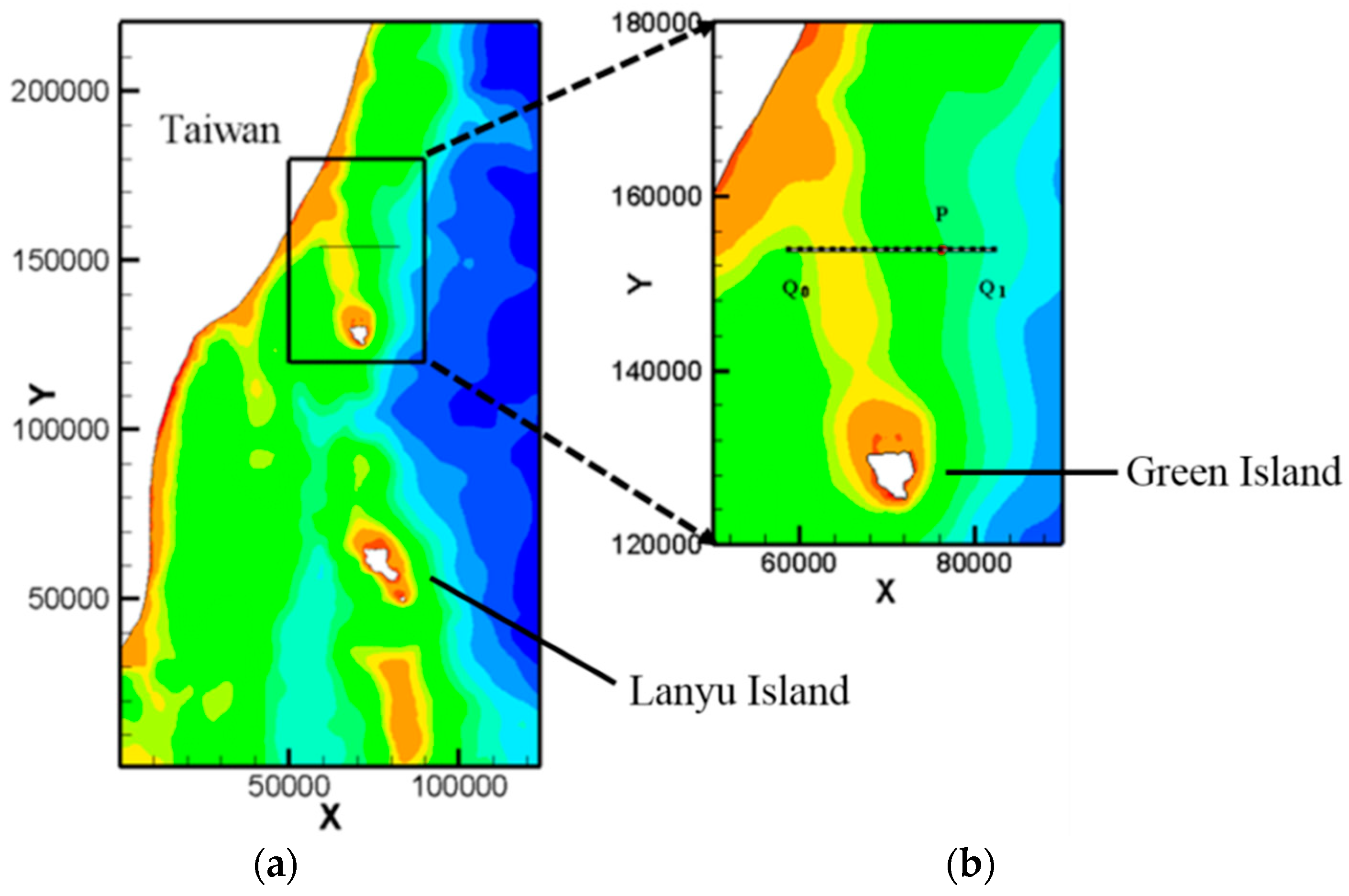
A high resolution (250–2250 m) SWEs model is used to investigate the hydrodynamic characteristics of the Kuroshio and downstream Green Island wakes. Green Island is located at (121°28′ E, 22°350′ N), 40 km off the southeastern coast of Taiwan. Figure 1a depicts the study area, the location of Lanyu Island and Green Island, and the bathymetry of the adjacent sea waters. The bathymetry of the study area varies from 400 to 5000 m, with an average value of about 2000 m. The bathymetry around the Green Island is within the range from 500 to 4000 m, with an average value of 2000 m. There are sea-mountains in the northwest of the Green Island where water depth varies from 200 to 400 m.
However, Kuroshio is a sub-surface flow where flow mainly occurs at the top 400 m layer of water with an average current speed around 1.0 m/s; water below 800 m is essentially motionless [17]. Therefore, we limit the bathymetry ranging from 10 to 360 m as the redefined bathymetry from the ETOPO1 (1 Arc-Minute Global Relief Model) in the simulations. Figure 1b depicts the computational meshes. It contains 50,842 nodes and 101,125 triangles. Spatial resolution varies from 250 to 2250 m. Fine meshes are employed near Lanyu Island and Green Island since flow field is expected to change dramatically in these areas. The increment of time step Δt = 45 s is used in the computations. The eight-day simulation of typhoon Soulik takes about 40 h on a personal computer equipped with an Intel(R) CoreTM i7-4700HQ [email protected].
The flow field data of HYCOM (hybrid coordinate ocean model) on 7 November 2014 after interpolation to the model grids, shown in Figure 1b, is utilized to initiate the flows. The choice of this particular flow field as the initial condition is based on the hypothesis proposed by Zheng and Zheng [43] in which the downstream Green Island wakes are prone to occur when Kuroshio mainstream heads on the island. Figure 2 shows the boundaries of the study domain. is the land boundary where no flux and free-slip boundary condition is applied, is the open boundary where the radiation boundary conditions are specified, and , , and are the velocity boundaries using the flow field data from HYCOM on 7 November 2014.
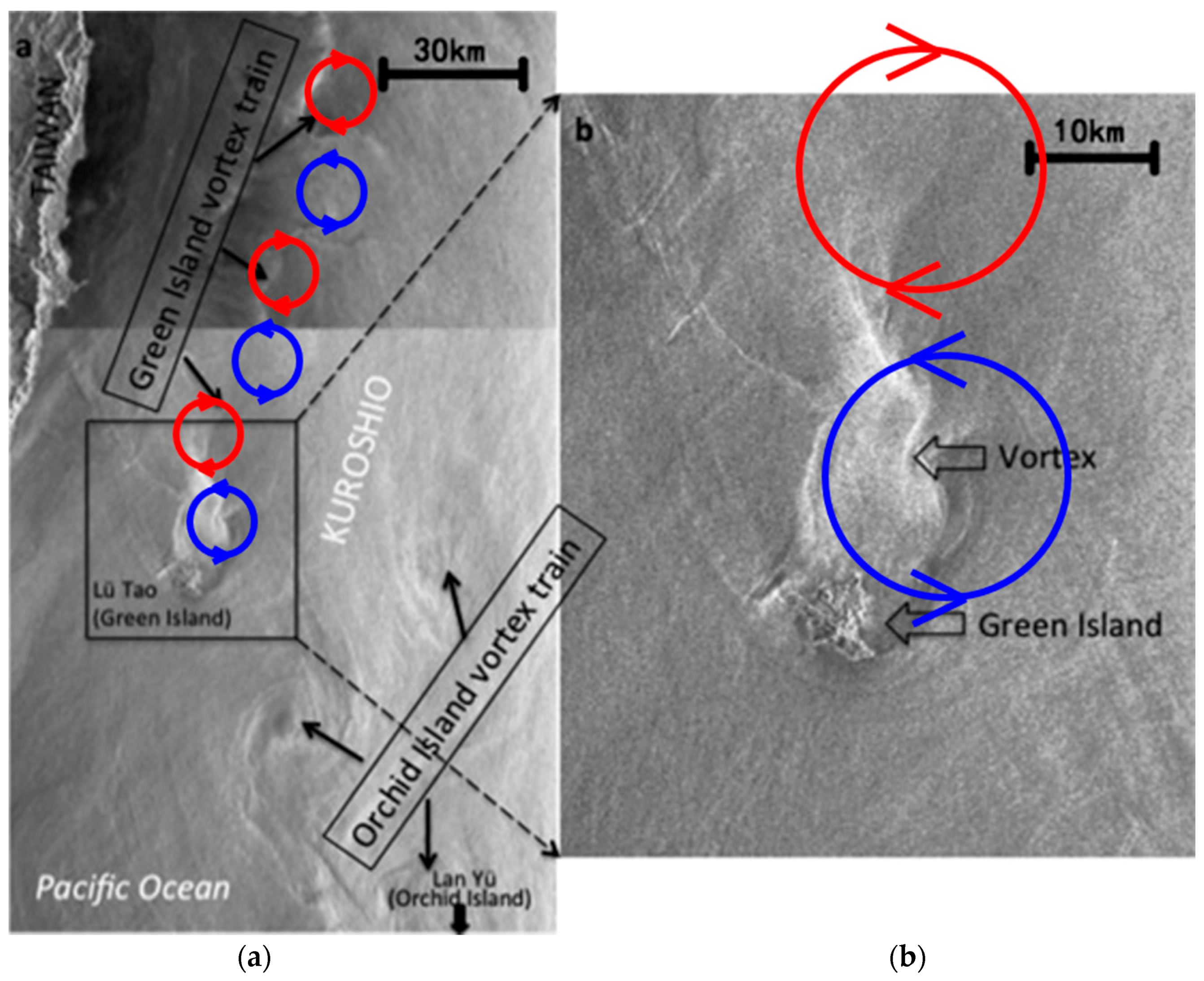
Figure 3 shows a composite ERS-1 SAR (European Remote Sensing satellite1, Synthetic Aperture Radar) image of downstream island vortex trains of Lanyu Island and Green Island taken with one week interval sequentially between 17:01 UT 25 September (lower) and 19:02 UT 2 October (top), 1996. Two downstream island vortex trains are clearly seen. One a small distance from the coast, called the Lanyu Island (also called the Orchid Island) vortex train, occurs downstream of Lanyu Island (a little beyond the southern boundary of the image), and consists of three vortexes, two cyclonic appearing as bright shading and one anticyclonic appearing as dark shading vortexes. Another near the eastern coast of Taiwan, called the Green Island vortex train, occurs downstream of Green Island, and consists of three pairs of cyclonic vortexes (bright center) and anticyclonic vortexes (dark center). Spatial and temporal scales of downstream Green Island wakes due to passing of the Kuroshio has been numerically studied [19]. The main difference between Liang et al. [19] and the present study lies in a constant inflow used in Liang et al. is replaced by a spatial varying inflow from HYCOM in the present study.
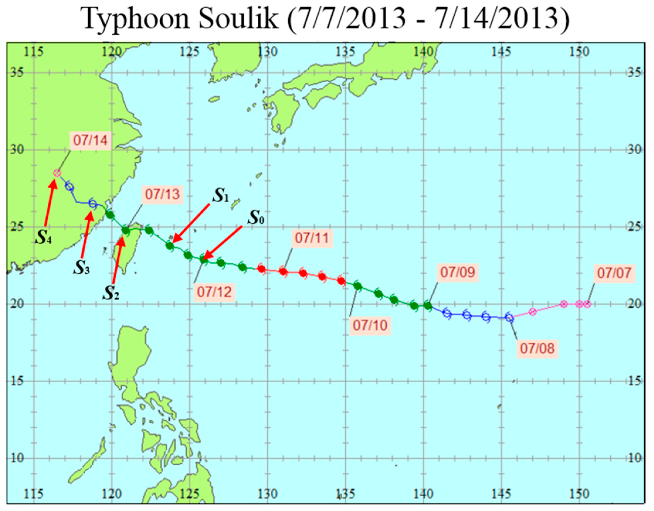
The SWEs model is applied to simulation the typhoon Soulik event. Typhoon Soulik hit the Taiwan area during 7 to 14 July 2013. Figure 4 depicts the track of typhoon Soulik. Typhoon Soulik, developed from a tropical depression on 7 July 2013 through a tropical storm, moderate typhoon, severe typhoon, and then decreased its strength and made landfall on Taiwan on 7 December 2013. The typhoon Soulik data with temporal intervals of every 6 h are from the CWB of Taiwan, which are computed by the NFS (non-hydrostatic forecast system). NFS uses the structured orthogonal meshes; however, the SWEs model uses the unstructured triangular meshes. Therefore, wind data needs to be interpolated into the computational nodes of the SWEs model. The IDW (inverse distance weighted interpolation [44]) is employed to interpolate the data from NFS into nodal points of the SWEs model. In this study, the 5-km resolution typhoon Soulik data is used. The maximum wind speed of typhoon Soulik is 51 m/s, categorized as a severe typhoon. The closest distance of typhoon to Green Island is about 250 km. The maximum wind speed of the model area is 17 m/s and the average value is smaller than 10 m/s.
Figure 5a depicts the global view of the study area, where the enclosed region near the Green Island indicates the sub-domain that will be presented in the succeeding plots of the downstream recirculation and island wakes. Figure 5b depicts the local view of the sub-domain as well as the location of the cross section and monitor point P at downstream Green Island, where time series of flow quantities are presented and analyzed. Length of is 20 km. It is located about 22 km downstream the Green Island.
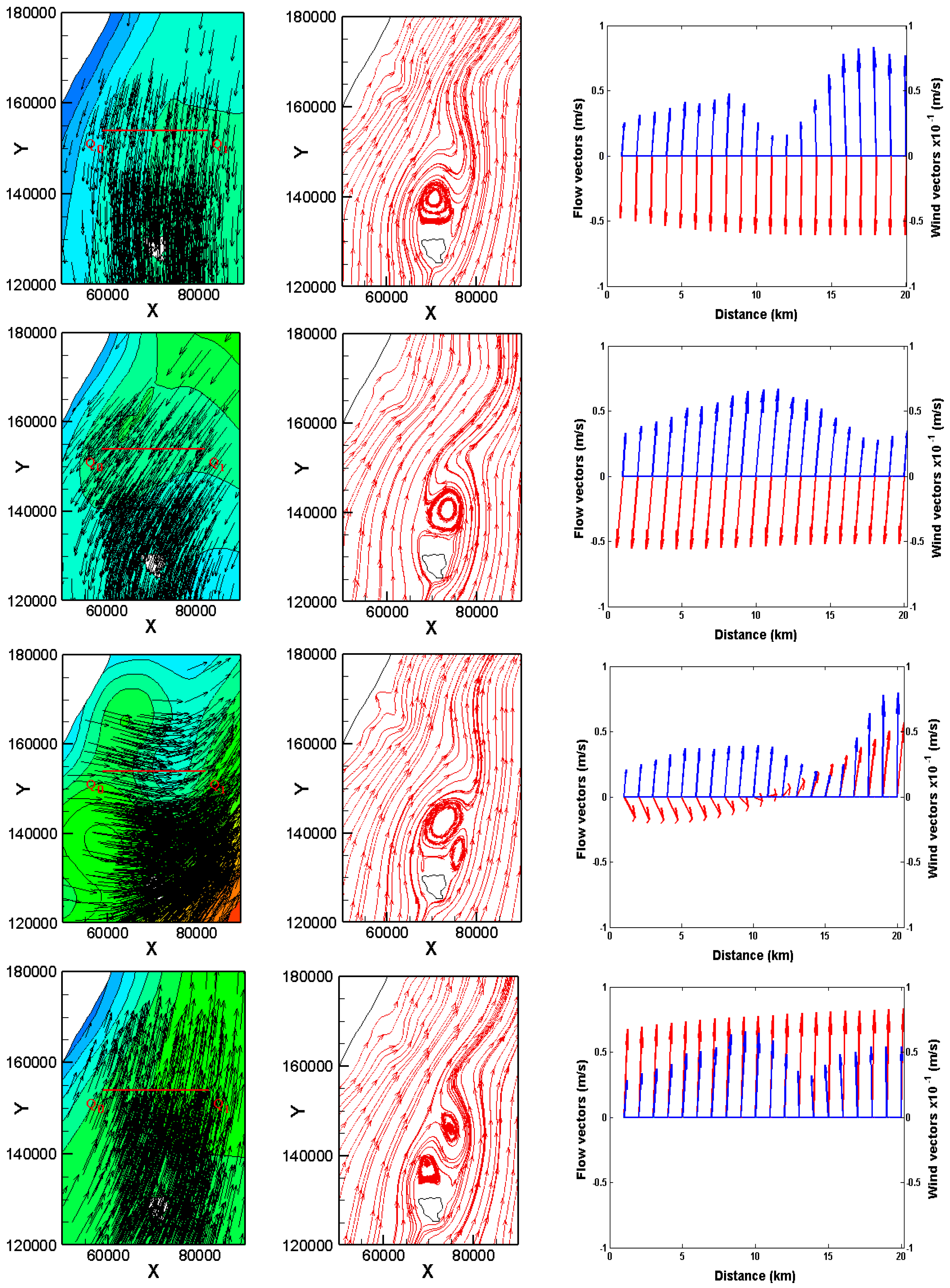
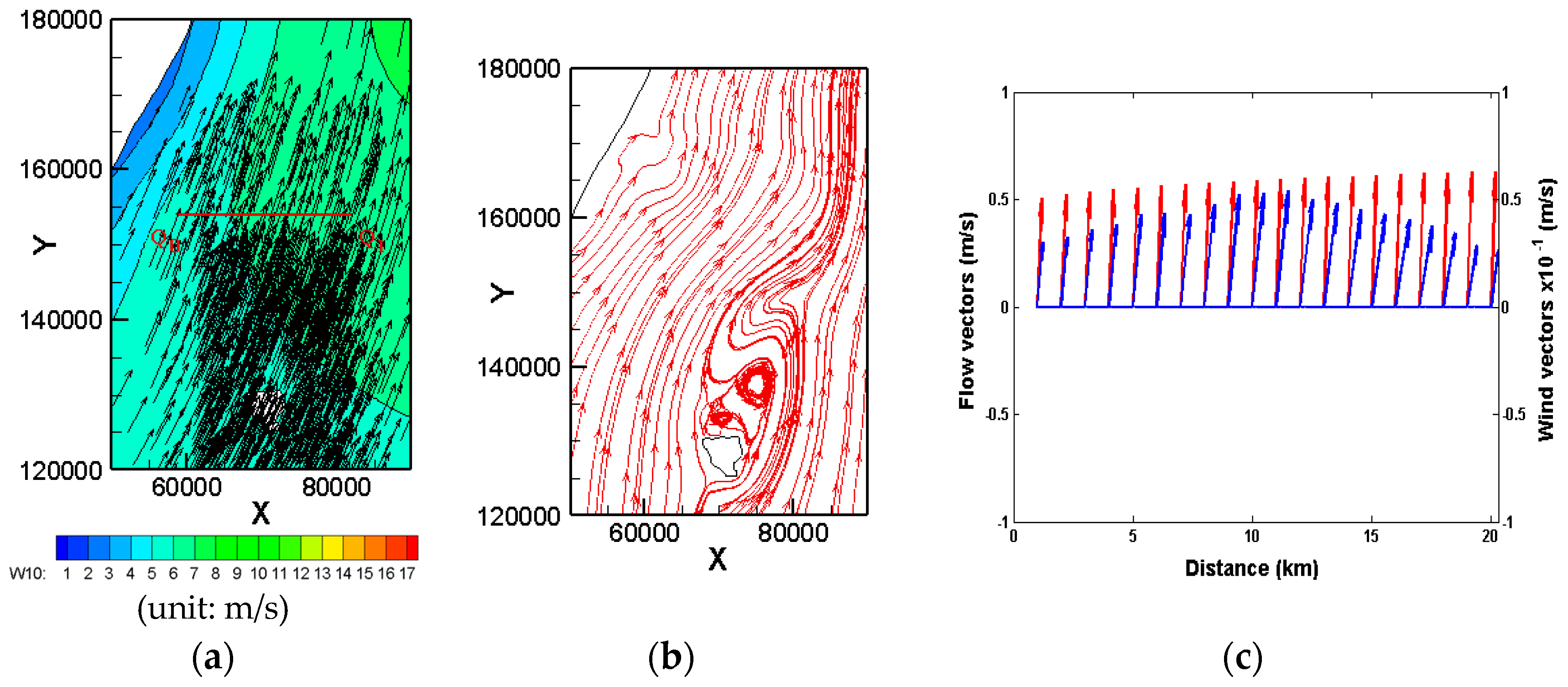
Figure 6 depicts the typhoon wind field and flow streamlines as well as vectors of wind (red) and flow (blue) along cross section at S0–S4 five time instances with a 12 h of increment, shown in Figure 5, where S0 represents 00:00 of 12 July, S1 12:00 of 12 July, S2 00:00 of 13 July, S3 12:00 of 13 July, and S4 00:00 of 14 July 2013, respectively. As can be seen, the downstream island wakes are well reproduced. The flow field is affected by the typhoon, especially in the shallow water area and the lee of the islands. Interactions of Kuroshio and downstream island wakes with typhoon are obvious. When typhoon approaches the study area, because of the cyclonic rotation and southward winding of typhoon, Kuroshio current decreases. At S3, we can see the moment when the center of the typhoon is closest to the Green Island. The wind starts to change its direction and to blow northward. Comparing flow vectors along cross section at S2 with that at S1 and S3 of Figure 6, it is noticed that downstream island wakes are significantly affected. Kuroshio currents increase after S2 due to the northward winding and resumes its normal flow condition after typhoon passes far away.
Figure 7a illustrates the location of 22.84° N (y = 150 km) cross section, where black dots denote the position of TOROS data, and Figure 7b,c depicts the comparison of the TOROS-observed surface currents with the computed flow vectors along the 22.84° N cross section at S0–S4: five time instances. Since TOROS data are the surface flow quantities, they are larger than the depth-averaged model predictions, in general. Moreover, the left one-third of the cross section (0–20 km) is right in the lee of Green Island. The meandering downstream island wakes are observed in the modelling, but not present in the TOROS data, because of its coarse spatial resolution (~10 km). However, computed results show Kuroshio currents increase when flow is in the same direction as the counterclockwise rotation of typhoon, and vice versa. This finding is consistent with the TOROS measured datasets [45].
3.2. Effect of Model Typhoon on Green Island Wakes
Figure 8 depicts flow streamlines around the Green Island of no wind forcing in a period of vortex shedding. There are small recirculations in the lee of Green Island. Its size is about the size of the island (~8 km). A well-organized coherent and alternating asymmetric meandering eddies in the lee of the Green Island is reproduced, which has been observed in field measurement [17] and satellite images [19,43]. In this study, simulation using the boundary conditions from HYCOM produces a more realistic Kuroshio flow and downstream Green Island wakes.
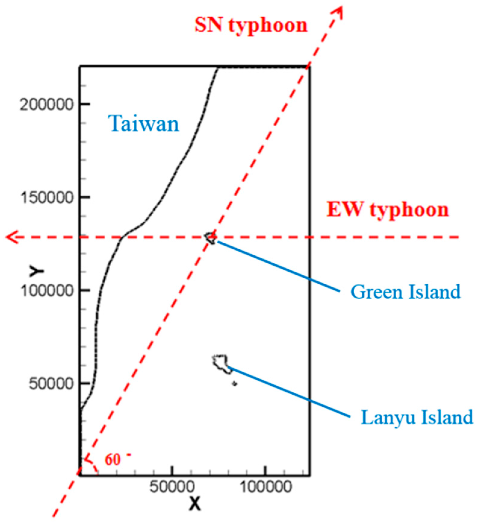
According to the statistical analysis of typhoons from 1911 to 2010 by the CWB of Taiwan, 83.6% of typhoons pass the eastern Taiwan coastal waters and 13.5% pass the western Taiwan coastal waters. Therefore, two typical tracks of typhoons, namely the SN typhoon (17% of total) moving from southwest to northeast and the EW typhoon (67% of total) moving from east to west, shown in Figure 9, are chosen to investigate the effect of typhoon on the Kuroshio and Green Island wakes. Two typical values of the typhoon moving speed, 2.5 m/s (9 km/h) and 5.0 m/s (18 km/h), are considered. Value of the radius of maximum wind speed Rmw = 50 km and pressure of typhoon center Pc = 950 hPa are used in the Holland’s wind field model. The resulting maximum of W10 is about 47 m/s.
In order to better quantify the net influence of typhoon on Green Island wakes, we subtract the flow field of SN typhoon case and EW typhoon case with no wind forcing case. The net influence of typhoon on the flow field is defined by
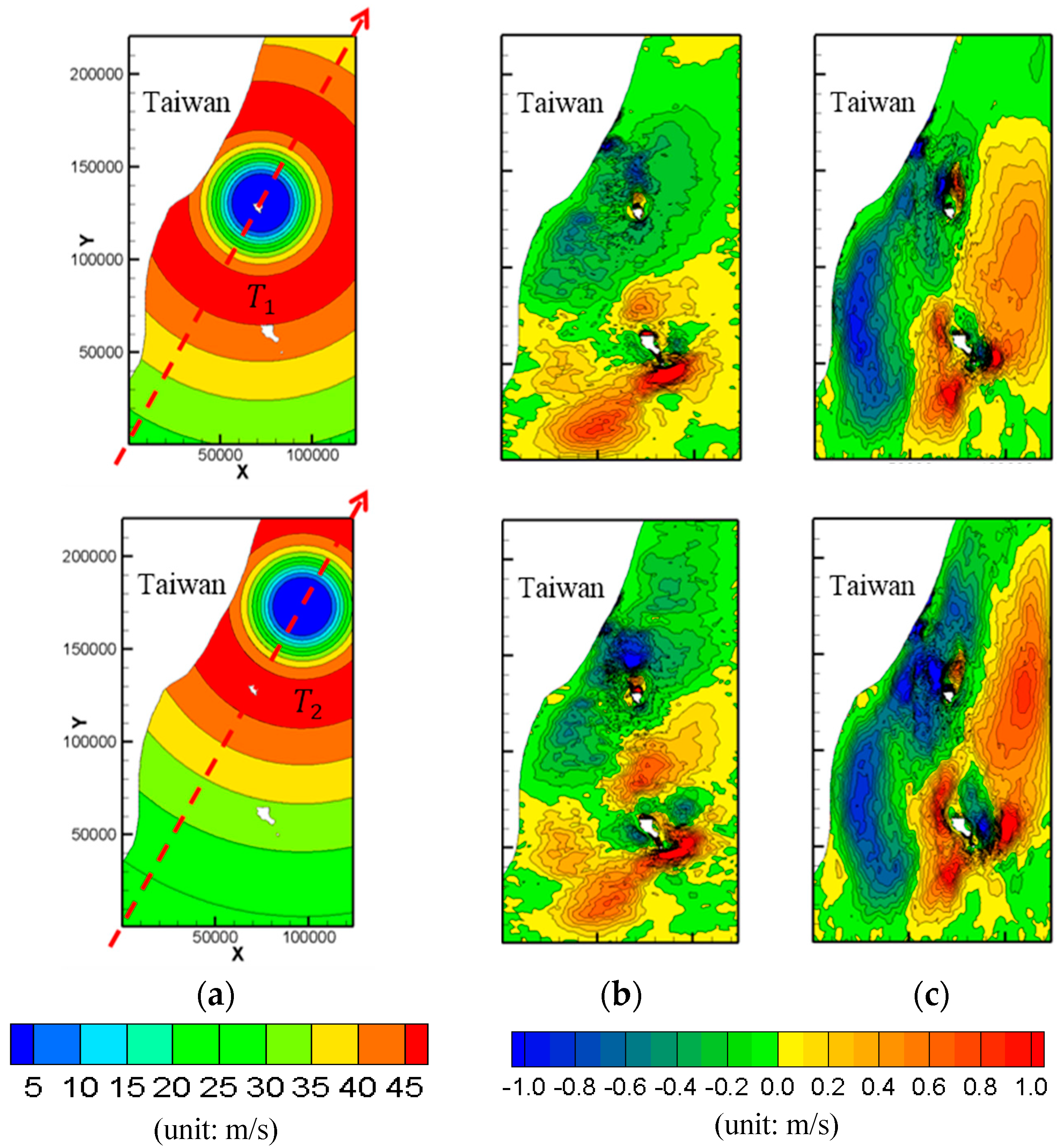
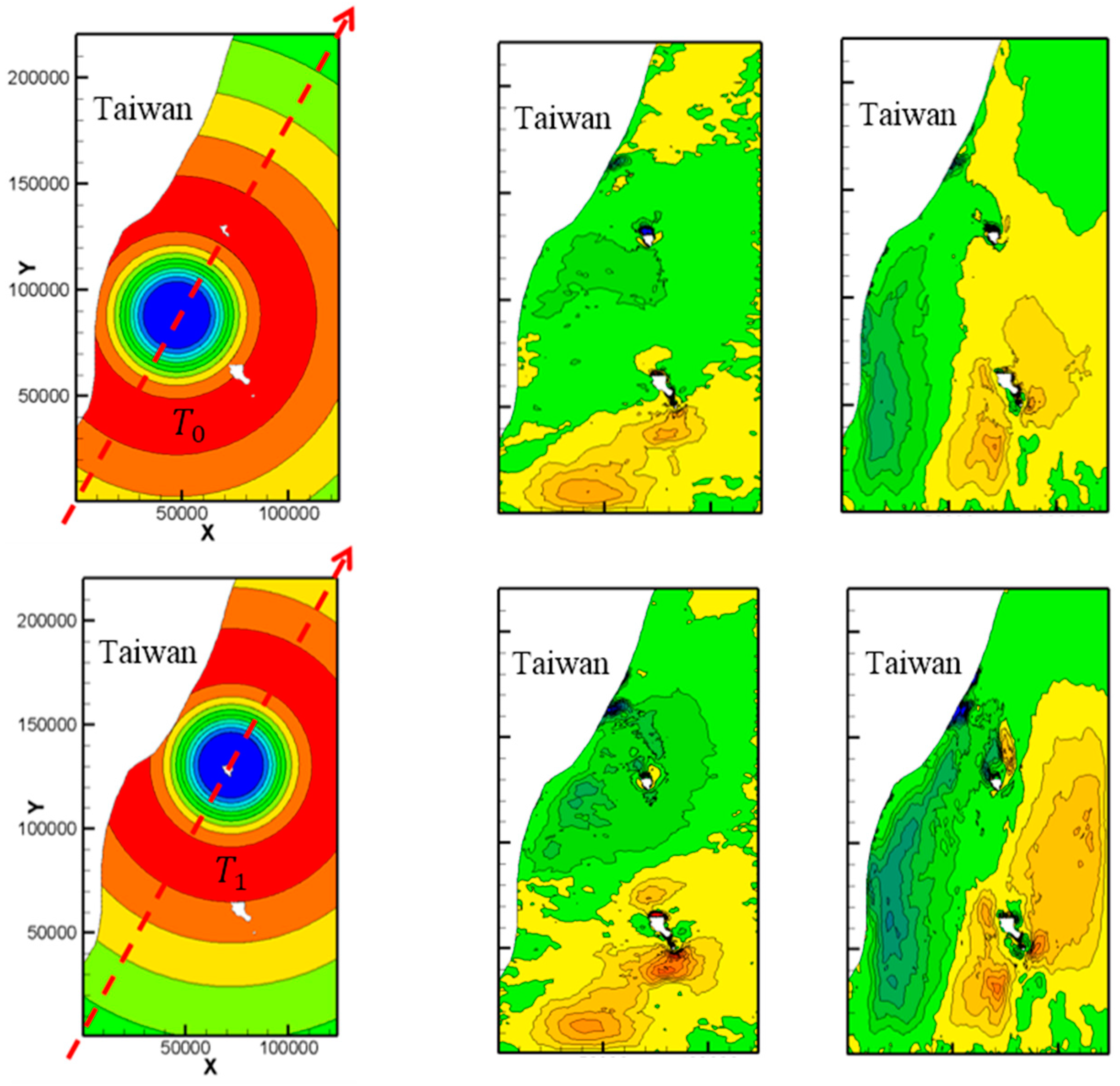
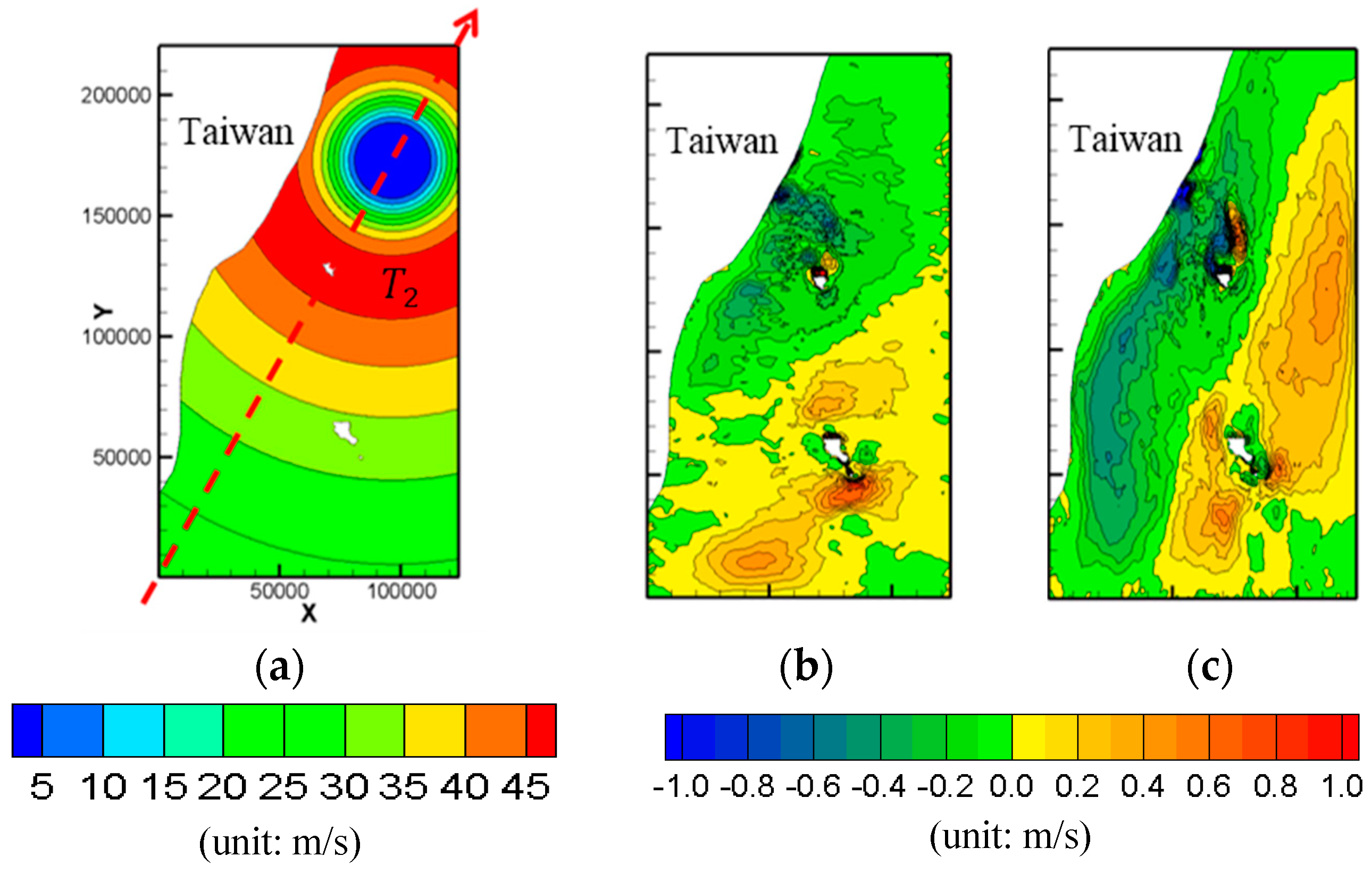
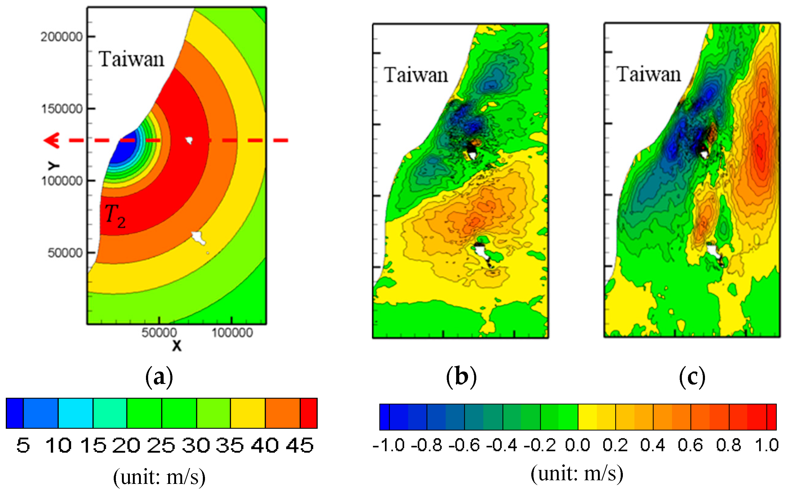
Figure 10 and Figure 11 show the “net” u- and v-contours of SN typhoon at T0–T2 three time instances as indicated in Figure 16. It is noted that the effect of typhoon on the y-component velocity are more pronounced than on the x-component velocity, because the direction of moving SN typhoon and the mainstream of Kuroshio is the same, in general. Due to the counterclockwise rotation of typhoon, flow accelerates (decelerates) when it flows in the favorable (adverse) direction of wind. For example, Figures 14 and 15 show that y-component velocity increases in the right of SN typhoon’s track and decreases in the left of SN typhoon’s track, the so called rightward bias phenomenon. The rightward bias phenomenon of u contours is not as evident as v contours, since the northeastward Kuroshio and x-component wind forcing are not in the same or opposite direction.
Comparing Figure 10 with Figure 11, we notice that the impact of the slow-moving typhoon (WT = 2.5 m/s) is more significant than the fast-moving typhoon (WT = 5.0 m/s), especially in the y-component velocity, when the typhoon moves in favor of the Kuroshio mainstream direction. When the typhoon moves slowly, it takes a longer time to travel the same distance. Therefore, more momentum and energy are input to water, and water takes more time to respond to the wind forcing.
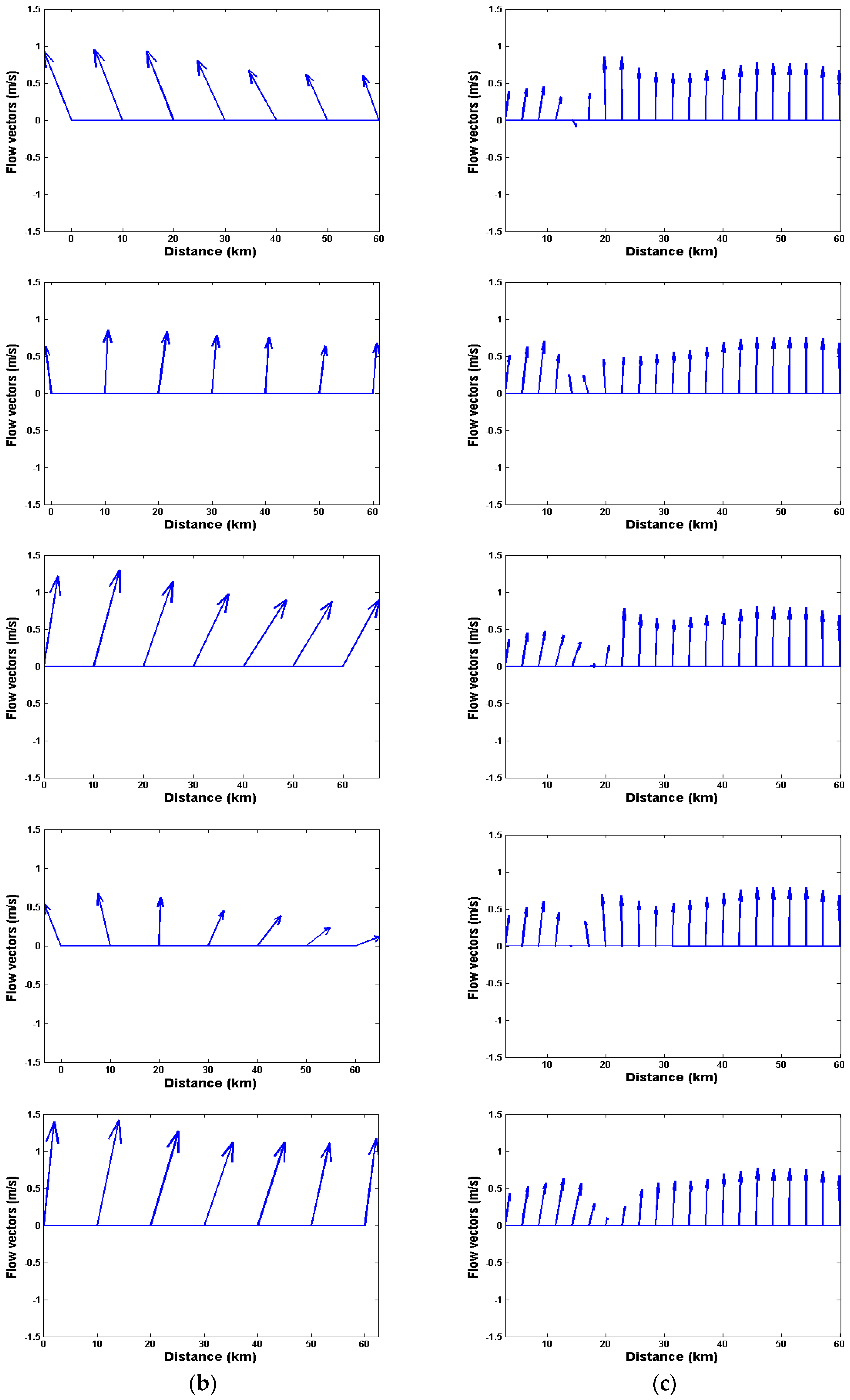
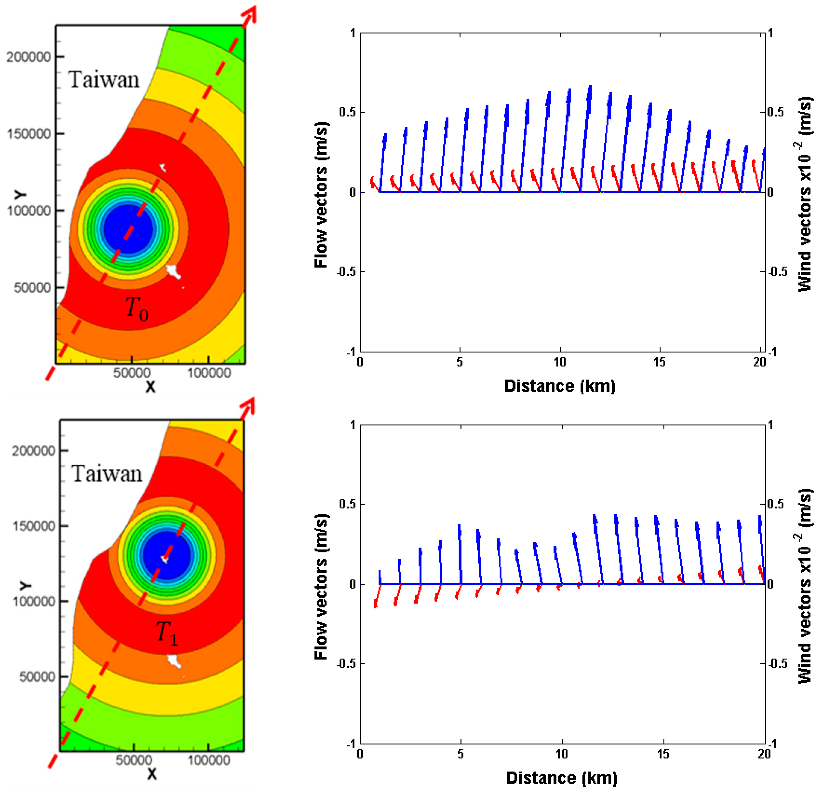
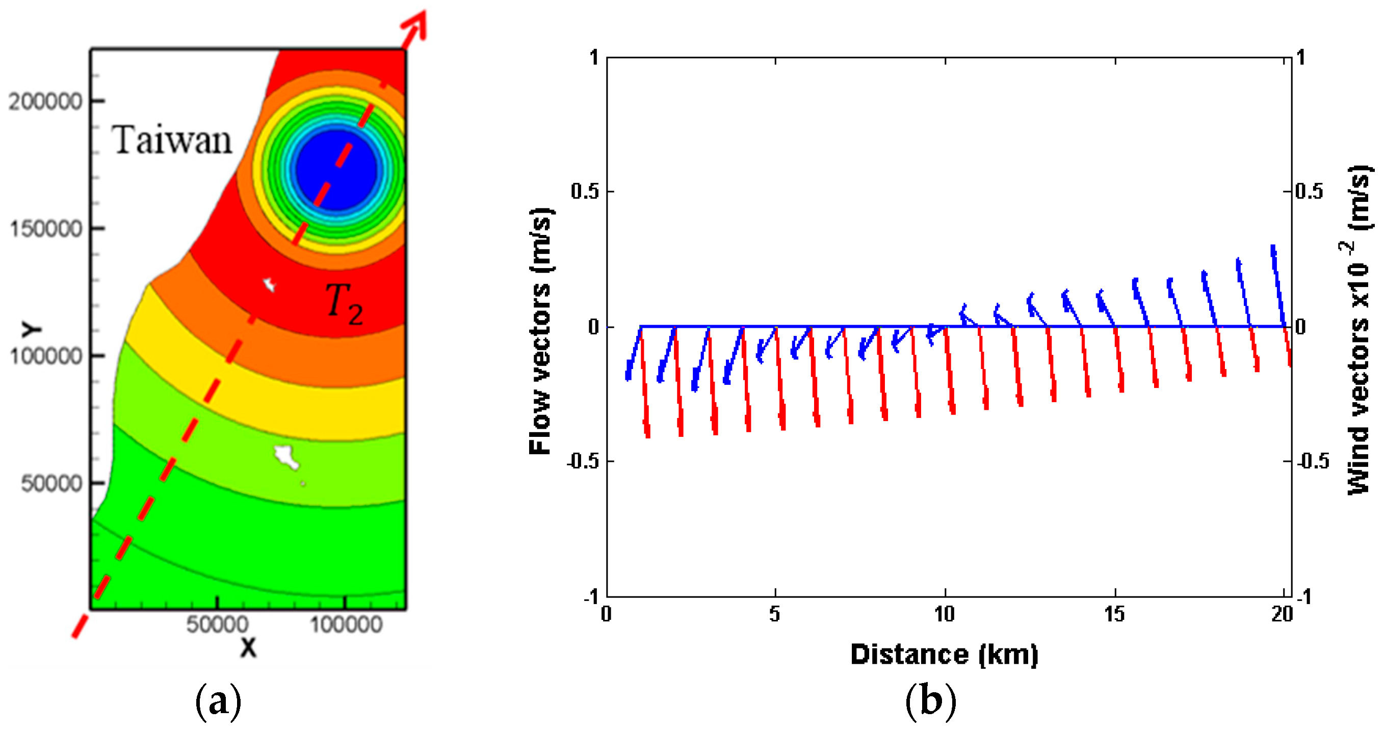
Figure 12 plots the wind field as well as wind vectors (red) and flow (blue) vectors along at T0–T2 three time instances. The flow field and downstream island wakes are significantly affected by the northeastward typhoon. Kuroshio currents increase as the typhoon approaches and decrease as the typhoon passes away.
Figure 13 and Figure 14 plot the “net” u- and v-contours of EW typhoon at T0–T2 three time instances indicated in Figure 16. The rightward bias feature due to the counterclockwise rotation of typhoon is evident, especially for the slow moving typhoon and y-component velocities. Comparing Figure 10 and Figure 11 with Figure 13 and Figure 14, the impact of SN typhoon on the Kuroshio and downstream Green Island wakes is apparently more significant than EW typhoon. The effect of the typhoon strengthens when the typhoon moves in favor of the Kuroshio and weakens when the typhoon moves against the Kuroshio.
Figure 15 plots the wind field as well as wind vectors (red) and flow vectors (blue) along at T0–T2 three time instances of the EW typhoon case. The flow field and downstream island wakes are also significantly affected by the EW typhoon. Kuroshio currents decrease as the typhoon approaches and increase in a short period as the typhoon passes away.
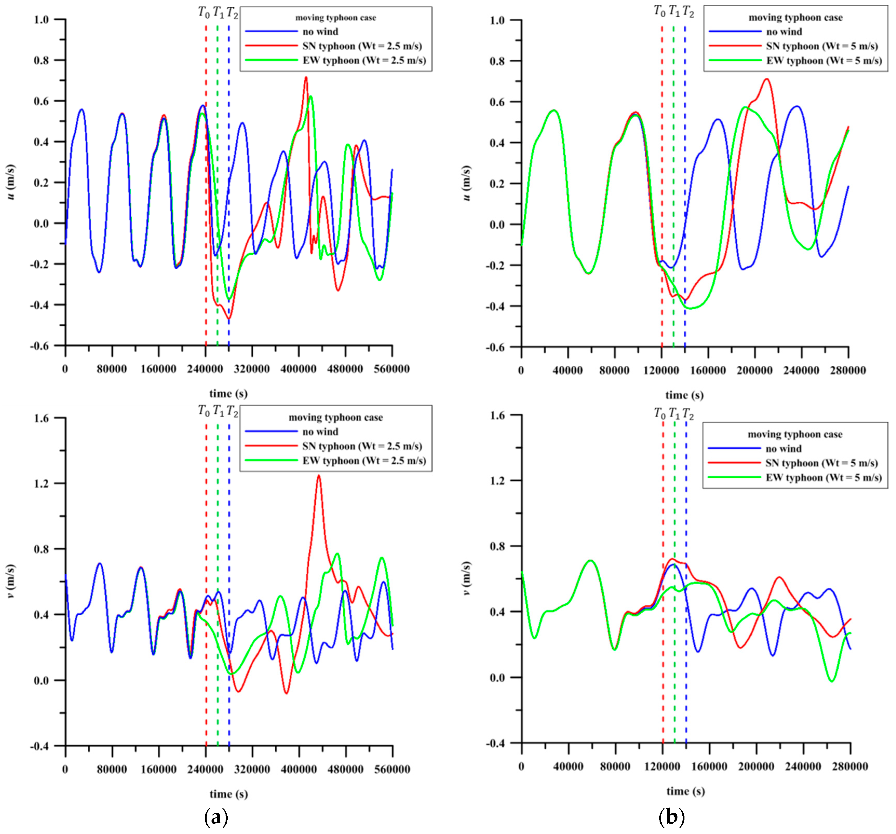
Figure 16 shows a comparison of time series of u and v of the monitor point P of no wind forcing case and SN typhoon case with (a) WT = 2.5 m/s and (b) WT = 5.0 m/s, respectively. Three vertical lines are drawn and represent the three time instances. The first time instance (T0), represented by the red vertical dashed line, indicates the time instance when the typhoon is located 50 km southwest of Green Island. The second time instance (T1), represented by the green vertical dashed line, indicates the moment when the typhoon passes the Green Island. The third time instance (T2), represented by the blue vertical dashed line, indicates the time instance when the typhoon is located 50 km northeast of Green Island. This shows that the typhoon has little influence on the flow field near P when it approaches P and is far away from P. However, the influence of the typhoon increases as the typhoon approaches P, and remains significant in a short period after the typhoon has passed far away from P.
4. Conclusions
Safety, maintenance, and operations of Kuroshio power plant may be subjected to impacts from earthquakes, typhoons, climate change, and other natural factors. Typhoons have a significant impact on the physical and chemical characteristics of the water of the Kuroshio. A shallow water model based on the shallow water equations and the space–time least-squares finite-element method has been developed. The model has been applied to study the hydrodynamics of Kuroshio and Green Island wakes with a small computational domain (72 km × 156 km) and coarse mesh resolution [19,25] (500–3500 m). The spatial and temporal scales of meandering downstream Green Island wakes have been quantified and compared with the in-situ measurements and satellite images. Special efforts of the present study are made to refine the model, including to integrate Holland’s wind field model [35], to use a larger computational domain (124 km× 220 km) with a finer mesh resolution (250–2250 m), and to use flow field from HYCOM as the initial and boundary conditions to drive the flows.
A high resolution (250–2250 m) shallow-water model is used to investigate effect of typhoon on the hydrodynamics of the Kuroshio and Green Island wakes. In the first case, we simulate the typhoon Soulik event to validate the applicability of the SWEs model. Computed results indicate that salient characteristics of Kuroshio and meandering downstream island wakes seem less affected by the typhoon because typhoon Soulik is 250 km away Green Island and wind speed is smaller than 10 m/s near the region of Green Island. However, Kuroshio currents increase when flow is in the same direction as the counterclockwise rotation of typhoon, and vice versa. This finding is consistent with the TOROS observed dataset [45].
In the second case, the SWEs model, forced by the Kuroshio and Holland’s wind field model, successfully reproduces the downstream recirculation and meandering vortex streets. Kuroshio and the downstream Green Island wakes are found to be significantly affected by the moving typhoon that passes the Green Island directly, especially for the shallow waters and the lee of the islands. Computed results clearly reveal the rightward bias phenomenon—due to the counterclockwise rotation of the typhoon, Kuroshio currents increase in the right of the moving typhoon’s track and decrease in the left of the moving typhoon’s track. Computed results also show that the slower the moving typhoon, the more significant is the impact of the typhoon on the Kuroshio and downstream Green Island wakes.
Acknowledgments
This study is supported by the MOST project under the grants of MOST 105-2221-E-019-022-MY2 and MOST 105-2221-E-019-043-MY2.
Author Contributions
Tai-Wen Hsu and Shin-Jye Liang proposed the method and wrote this paper. Meng-Hsien Chou and Shin-Jye Liang surveyed literatures, implemented the algorithms, performed the simulations, and analyzed the modeling results. Wei-Ting Chao helped with paper formatting and revising. All authors contributed to the discussion of the results and the writing of the manuscript.
Conflicts of Interest
The authors declare no conflict of interest.
References
- Zdravkovich, M.M. Flow around Circular Cylinders; Applications, Oxford University Press: Oxford, UK, 2003; Volume 2, ISBN 9780198565611. [Google Scholar]
- Chelton, D.B.; Schlax, M.G.; Samelson, R.M. Global observations of nonlinearmesoscale eddies. Prog. Oceanogr. 2011, 91, 167–216. [Google Scholar] [CrossRef]
- Nunalee, C.G.; Basu, S. On the periodicity of atmospheric von Kármán vortex streets. Environ. Fluid Mech. 2014, 14, 1335–1355. [Google Scholar] [CrossRef]
- Roshko, A. On the wake and drag of bluff bodies. J. Aeronaut. Sci. 1955, 22, 124–132. [Google Scholar] [CrossRef]
- Tritton, D.J. Experiments on the flow past a circular cylinder at low Reynolds numbers. J. Fluid Mech. 1959, 6, 547–567. [Google Scholar] [CrossRef]
- Williamson, C.H. Vortex dynamics in the cylinder wake. Annu. Rev. Fluid Mech. 1996, 28, 477–539. [Google Scholar] [CrossRef]
- Hubert, L.; Krueger, A. Satellite pictures of mesoscale eddies. Mon. Weather Rev. 1962, 90, 457–463. [Google Scholar] [CrossRef]
- Li, X.; Clemente-Colón, P.; Pichel, W.G.; Vachon, P.W. Atmospheric vortex streets ona RADARSAT SAR image. Geophys. Res. Lett. 2000, 27, 1655–1658. [Google Scholar] [CrossRef]
- Thomson, R.E.; Gower, J.F.; Bowker, N.W. Vortex streets in the wake of the AleutianIslands. Mon. Weather Rev. 1977, 105, 873–884. [Google Scholar] [CrossRef]
- Young, G.S.; Zawislak, J. An observational study of vortex spacing in island wake vortexstreets. Mon. Weather Rev. 2006, 134, 2285–2294. [Google Scholar] [CrossRef]
- Zheng, Q.; Lin, H.; Meng, J.; Hu, X.; Song, Y.T.; Zhang, Y.; Li, C. Submesoscale oceanvortex trains in the Luzon Strait. J. Geophys. Res. Oceans 2008, 113, C0403-1–C04032-12. [Google Scholar] [CrossRef]
- Barkley, R.A. Johnston atolls wake. J. Mar. Res. 1972, 30, 201–216. [Google Scholar]
- Dong, C.; McWilliams, J.C.; Shchepetkin, A.F. Island wakes in deep water. J. Phys. Oceanogr. 2007, 37, 962–981. [Google Scholar] [CrossRef]
- Heywood, K.J.; Stevens, D.P.; Bigg, G.R. Eddy formation behind the tropical island ofAldabra. Deep-Sea Res. Part I 1996, 43, 555–578. [Google Scholar] [CrossRef] [Green Version]
- Ruscher, P.H.; Deardorff, J.W. A numerical simulation of an atmospheric vortex street. Tellus A 1982, 34, 555–566. [Google Scholar] [CrossRef]
- Wolanski, E.; Imberger, J.; Heron, M. Island wakes in shallow coastal waters. J. Geophys. Res. Oceans 1984, 89, 10553–10569. [Google Scholar] [CrossRef]
- Chang, M.H.; Tang, T.Y.; Ho, C.R.; Chao, S.Y. Kuroshioinduced wake in the lee of GreenIsland off Taiwan. J. Geophys. Res. Oceans 2013, 118, 1508–1519. [Google Scholar] [CrossRef]
- Hsin, Y.C.; Wu, C.R.; Shaw, P.T. Spatial and temporal variations of the Kuroshio east ofTaiwan, 1982–2005: A numerical study. J. Geophys. Res. Oceans 2008, 113, C04002-1–C04002-15. [Google Scholar] [CrossRef]
- Liang, S.J.; Lin, C.Y.; Hsu, T.W.; Ho, C.R.; Chang, M.H. Numerical study of vortexcharacteristics near Green Island, Taiwan. J. Coast. Res. 2013, 29, 1436–1444. [Google Scholar] [CrossRef]
- Gunduz, M.; Özsoy, E. Modelling seasonal circulation and thermohaline structure of the Caspian Sea. Ocean Sci. 2014, 10, 459–471. [Google Scholar] [CrossRef]
- Suda, K. The Science of the Sea (Kaiyo-Kagaku); Kokin-Shoin: Tokyo, Japan, 1943. [Google Scholar]
- Sun, L.; Yang, Y.J.; Fu, Y.F. Impacts of typhoons on the Kuroshio large meander: Observationevidences. Atmos. Ocean. Sci. 2009, 2, 45–50. [Google Scholar] [CrossRef]
- Chen, C.T.A.; Liu, C.T.; Chuang, W.; Yang, Y.; Shiah, F.K.; Tang, T.; Chung, S. Enhancedbuoyancy and hence upwelling of subsurface Kuroshio waters after a typhoon in the southern East China Sea. J. Mar. Syst. 2003, 42, 65–79. [Google Scholar] [CrossRef]
- Chen, F. The Kuroshio Power Plant, The Kuroshio Power Plant; Springer: Singapore, 2013; ISBN 978-3-319-00822-6. [Google Scholar]
- Hsu, T.W.; Doong, D.J.; Hsieh, K.J.; Liang, S.J. Numerical study of Monsoon effecton Green Island Wake. J. Coast. Res. 2015, 31, 1141–1150. [Google Scholar] [CrossRef]
- Liu, K.K.; Gong, G.C.; Shyu, C.Z.; Pai, S.C.; Wei, C.L.; Chao, S.Y. Response of Kuroshioupwelling to the onset of the northeast monsoon in the sea north of Taiwan: Observations anda numerical simulation. J. Geophys. Res. Oceans 1992, 97, 12511–12526. [Google Scholar] [CrossRef]
- Buachart, C.; Kanok-Nukulchai, W.; Ortega, E.; Onate, E. A shallow watermodel by finite point method. Int. J. Comput. Meth. 2014, 11, 1350047-1–1350047-27. [Google Scholar] [CrossRef]
- Johnson, R. A Modern Introduction to the Mathematical Theory of Water Waves; Cambridge University Press: Cambridge, UK, 1997. [Google Scholar]
- Tan, W.Y. Shallow Water Hydrodynamics: Mathematical Theory and Numerical Solution fora Two-Dimensional System of Shallow-Water Equations; Elsevier: Singapore, 1992; ISBN 9780080870939. [Google Scholar]
- Vreugdenhil, C.B. Numerical Methods for Shallow-Water Flow; Springer Science & BusinessMedia: Singapore, 2013. [Google Scholar]
- Toro, E.F. Riemann Solvers and Numerical Methods for Fluid Dynamics; A Practical Introduction; Springer: New York, NY, USA, 1999. [Google Scholar]
- Toro, E.F. Shock-Capturing Methods for Free-Surface Shallow Flows; John Wiley & Sons: New York, NY, USA, 2001. [Google Scholar]
- Yulistiyanto, B.; Zech, Y.; Graf, W. Flow around a cylinder: Shallow-water modeling withdiffusion-dispersion. J. Hydraul. Eng. ASCE 1998, 124, 419–429. [Google Scholar] [CrossRef]
- Martin, J.L.; McCutcheon, S.C. Hydrodynamics and Transport for Water Quality Modeling; CRC Press: Boca Raton, FL, USA, 1998; ISBN 9780873716123. [Google Scholar]
- Holland, G.J.; Belanger, J.I.; Fritz, A. A revised model for radial profiles of hurricanewinds. Mon. Weather Rev. 2010, 138, 4393–4401. [Google Scholar] [CrossRef]
- Powell, M.D. Evaluations of diagnostic marine boundary-layer models applied to hurricanes. Mon. Weather Rev. 1980, 108, 757–766. [Google Scholar] [CrossRef]
- Zhang, H.; Sannasiraj, S. Wind wave effects on surface stress in hydrodynamic modeling. In Proceedings of the Eighth ISOPE Pacific/Asia Offshore Mechanics Symposium, Bangkok, Thailand, 10–14 November 2008; International Society of Offshore and Polar Engineers: Vancouver, BC, Canada, 2008. [Google Scholar]
- Gunzburger, M.D. Finite Element Methods for Viscous Incompressible Flows: A Guide to Theory; Practice, and Algorithms; Elsevier: Singapore, 2012; ISBN 9780323139823. [Google Scholar]
- Hughes, T.J.; Hulbert, G.M. Space-time finite element methods for elastodynamics: Formulationsand error estimates. Comput. Methods Appl. Mech. 1988, 66, 339–363. [Google Scholar] [CrossRef]
- Jiang, B.N. The Least-Squares Finite Element Method: Theory and Applications in Computational Fluid Dynamics and Electromagnetics; Springer Science & Business Media: Berlin, Germany, 1998; ISBN 978-3-662-03740-9. [Google Scholar]
- Laible, J.P.; Pinder, G.F. Solution of the shallow water equations by least squares collocation. Water Resour. Res. 1993, 29, 445–455. [Google Scholar] [CrossRef]
- Liang, S.J.; Hsu, T.W. Least-squares finite-element method for shallow-water equationswith source terms. Acta Mech. Sin. 2009, 25, 597–610. [Google Scholar] [CrossRef]
- Zheng, Z.W.; Zheng, Q. Variability of island-induced ocean vortex trains, in the Kuroshioregion southeast of Taiwan Island. Cont. Shelf Res. 2014, 81, 1–6. [Google Scholar] [CrossRef]
- Shepard, D. A two-dimensional interpolation function for irregularly-spaced data. In Proceedings of the 23rd ACM National Conference, New York, NY, USA, 27–29 August 1968; pp. 517–524. [Google Scholar]
- Lu, Y.C.; Liau, J.M.; Ou, S.H.; Lai, J.W.; Chou, M.H.; Hsu, T.W. Effects of typhoon onKuroshio current field. In Proceedings of the 7th Chinese-German Joint Symposium on Hydraulic and OceanEngineering, Leibniz Universitat Hannover, Hanover, Germany, 8–12 September 2014. [Google Scholar]
Figure 1.
(a) Schematic illustration of the study area and the bathymetry derived from the ETOPO1 and (b) computational meshes with fine meshes used in the coastal waters around Lanyu Island and Green Island.
Figure 1.
(a) Schematic illustration of the study area and the bathymetry derived from the ETOPO1 and (b) computational meshes with fine meshes used in the coastal waters around Lanyu Island and Green Island.
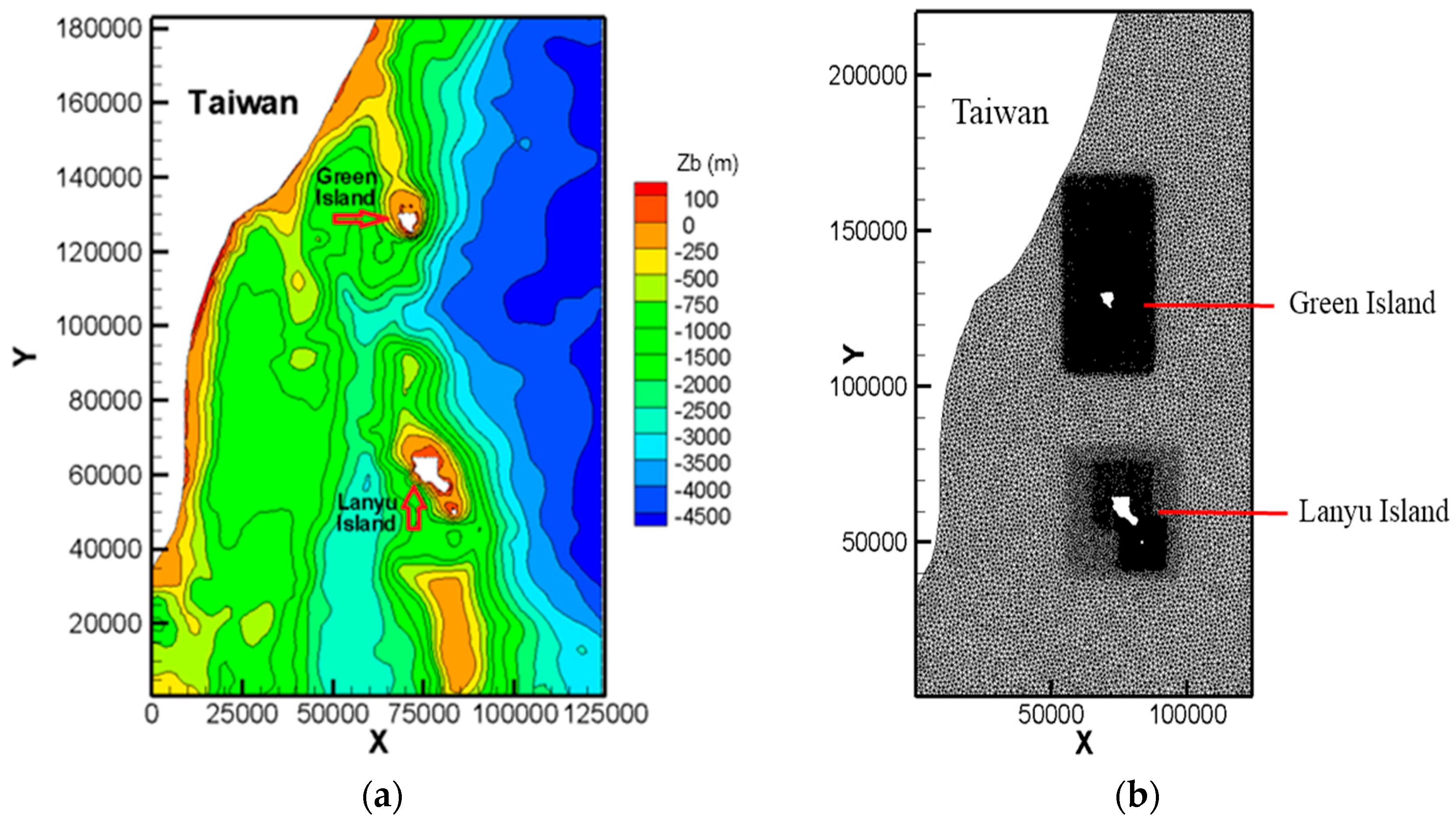
Figure 2.
Study domain and boundaries, as well as streamlines from the hybrid coordinate ocean model) (HYCOM).
Figure 2.
Study domain and boundaries, as well as streamlines from the hybrid coordinate ocean model) (HYCOM).
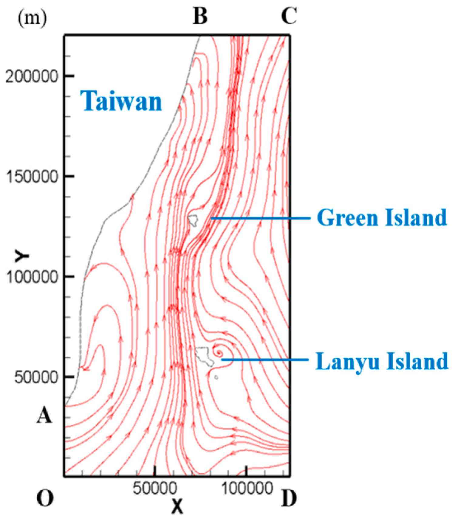
Figure 3.
(a) A composite ERS-1 SAR image of island-induced ocean vortex trains of Lanyu Island and Green Island taken at 17:01 UT 25 September (lower) and 19:02 UT 2 October (top), 1996. (b) Zoomed Green Island and head of vortex train (modified from Figure 2 of Zheng and Zheng [43]). Blue circle represents for cyclonic (bright shading) vortexes and red circle represents for anticyclonic (dark shading) vortexes.

Figure 4.
Track of typhoon Soulik from 7 to 14 June 2013, where symbol ![Atmosphere 09 00036 i001]() denotes the tropical depression with maximum wind speed Vmax < 17.2 m/s;
denotes the tropical depression with maximum wind speed Vmax < 17.2 m/s; ![Atmosphere 09 00036 i002]() the tropical storm, 17.2 m/s < Vmax < 32.6 m/s;
the tropical storm, 17.2 m/s < Vmax < 32.6 m/s; ![Atmosphere 09 00036 i003]() the moderate typhoon, 32.7 m/s < Vmax < 50.9 m/s;
the moderate typhoon, 32.7 m/s < Vmax < 50.9 m/s; ![Atmosphere 09 00036 i004]() a severe typhoon, 51 m/s < Vmax, and S0–S4 are the five time instances with a 12 h of increment to show the flow fields, see Figure 6, for example, S0 represents 00:00 of 12 July, S1 12:00 of 12 July, S2 00:00 of 13 July, S3 12:00 of 13 July and S4 00:00 of 14 July 2013, respectively. (Modified from CWB of Taiwan).
a severe typhoon, 51 m/s < Vmax, and S0–S4 are the five time instances with a 12 h of increment to show the flow fields, see Figure 6, for example, S0 represents 00:00 of 12 July, S1 12:00 of 12 July, S2 00:00 of 13 July, S3 12:00 of 13 July and S4 00:00 of 14 July 2013, respectively. (Modified from CWB of Taiwan).
 denotes the tropical depression with maximum wind speed Vmax < 17.2 m/s;
  the tropical storm, 17.2 m/s < Vmax < 32.6 m/s;
  the moderate typhoon, 32.7 m/s < Vmax < 50.9 m/s;
  a severe typhoon, 51 m/s < Vmax, and S0–S4 are the five time instances with a 12 h of increment to show the flow fields, see Figure 6, for example, S0 represents 00:00 of 12 July, S1 12:00 of 12 July, S2 00:00 of 13 July, S3 12:00 of 13 July and S4 00:00 of 14 July 2013, respectively. (Modified from CWB of Taiwan).
Figure 4.
Track of typhoon Soulik from 7 to 14 June 2013, where symbol ![Atmosphere 09 00036 i001]() denotes the tropical depression with maximum wind speed Vmax < 17.2 m/s;
denotes the tropical depression with maximum wind speed Vmax < 17.2 m/s; ![Atmosphere 09 00036 i002]() the tropical storm, 17.2 m/s < Vmax < 32.6 m/s;
the tropical storm, 17.2 m/s < Vmax < 32.6 m/s; ![Atmosphere 09 00036 i003]() the moderate typhoon, 32.7 m/s < Vmax < 50.9 m/s;
the moderate typhoon, 32.7 m/s < Vmax < 50.9 m/s; ![Atmosphere 09 00036 i004]() a severe typhoon, 51 m/s < Vmax, and S0–S4 are the five time instances with a 12 h of increment to show the flow fields, see Figure 6, for example, S0 represents 00:00 of 12 July, S1 12:00 of 12 July, S2 00:00 of 13 July, S3 12:00 of 13 July and S4 00:00 of 14 July 2013, respectively. (Modified from CWB of Taiwan).
a severe typhoon, 51 m/s < Vmax, and S0–S4 are the five time instances with a 12 h of increment to show the flow fields, see Figure 6, for example, S0 represents 00:00 of 12 July, S1 12:00 of 12 July, S2 00:00 of 13 July, S3 12:00 of 13 July and S4 00:00 of 14 July 2013, respectively. (Modified from CWB of Taiwan).
denotes the tropical depression with maximum wind speed Vmax < 17.2 m/s; the tropical storm, 17.2 m/s < Vmax < 32.6 m/s; the moderate typhoon, 32.7 m/s < Vmax < 50.9 m/s; a severe typhoon, 51 m/s < Vmax, and S0–S4 are the five time instances with a 12 h of increment to show the flow fields, see Figure 6, for example, S0 represents 00:00 of 12 July, S1 12:00 of 12 July, S2 00:00 of 13 July, S3 12:00 of 13 July and S4 00:00 of 14 July 2013, respectively. (Modified from CWB of Taiwan).
Figure 5.
(a) Global view of the study area, where the enclosed region near the Green Island indicates the sub-domain that will be presented in the succeeding plots of the downstream recirculation and island wakes, and (b) local view of the sub-domain as well as location of the cross section and monitor point P at downstream Green Island. Length of is 20 km. It locates about 22 km downstream the Green Island.

Figure 6.
(a) W10 vectors and contours (unit: m/s), (b) flow streamlines, and (c) wind vectors (red) and flow vectors (blue) of cross section at S0–S4 five time instances of the typhoon Soulik, see Figure 5.
Figure 6.
(a) W10 vectors and contours (unit: m/s), (b) flow streamlines, and (c) wind vectors (red) and flow vectors (blue) of cross section at S0–S4 five time instances of the typhoon Soulik, see Figure 5.


Figure 7.
(a) Location of the 22.84° N (y = 150 km) cross section, where black dots denote the position of TOROS data. (b) and (c) depict comparison of flow vectors of TOROS data and model predictions along 22.84° N cross section at S0–S4: five time instances, see Figure 5.
Figure 7.
(a) Location of the 22.84° N (y = 150 km) cross section, where black dots denote the position of TOROS data. (b) and (c) depict comparison of flow vectors of TOROS data and model predictions along 22.84° N cross section at S0–S4: five time instances, see Figure 5.
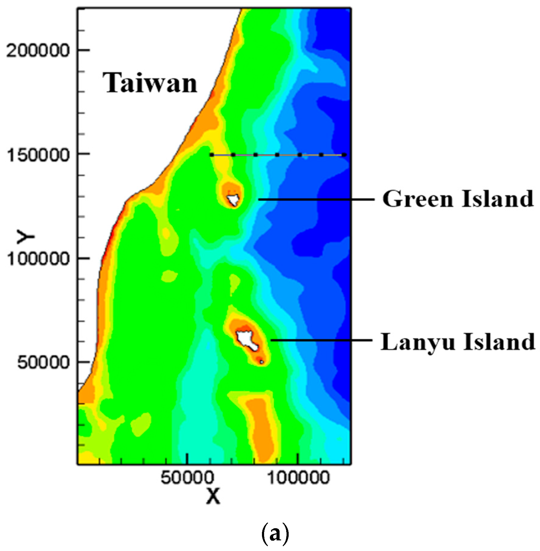

Figure 8.
Flow streamlines of the Green Island wakes in the no wind forcing case.
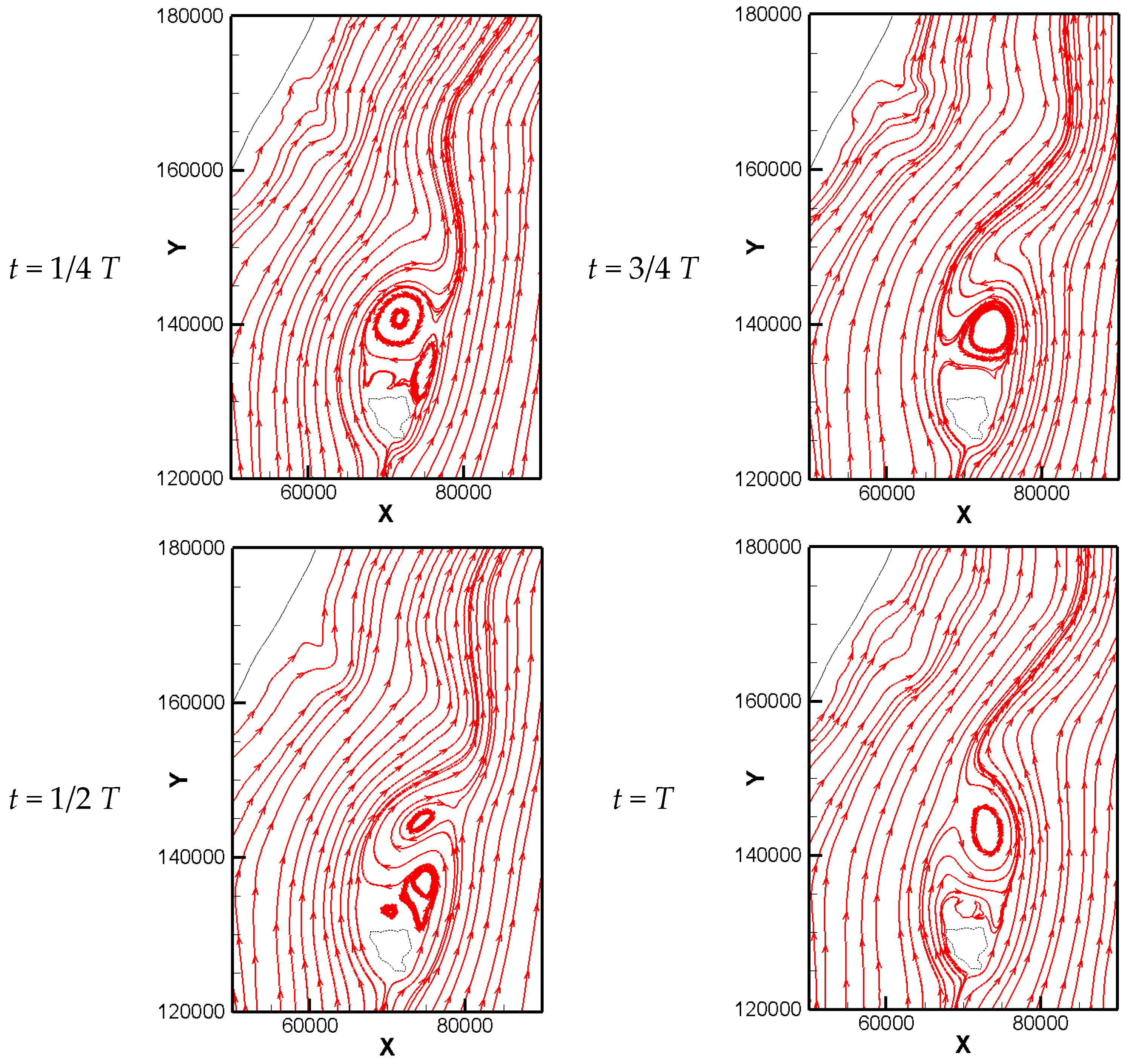
Figure 9.
Schematic diagram of the study domain and track of SN and EW typhoon.

Figure 10.
Contours of (a) W10, “net” (b) u-, and (c) v-contours of (unit: m/s) SN typhoon with moving speed WT = 2.5 m/s at T0–T2 three time instances indicated by the three vertical lines of Figure 16a.
Figure 10.
Contours of (a) W10, “net” (b) u-, and (c) v-contours of (unit: m/s) SN typhoon with moving speed WT = 2.5 m/s at T0–T2 three time instances indicated by the three vertical lines of Figure 16a.
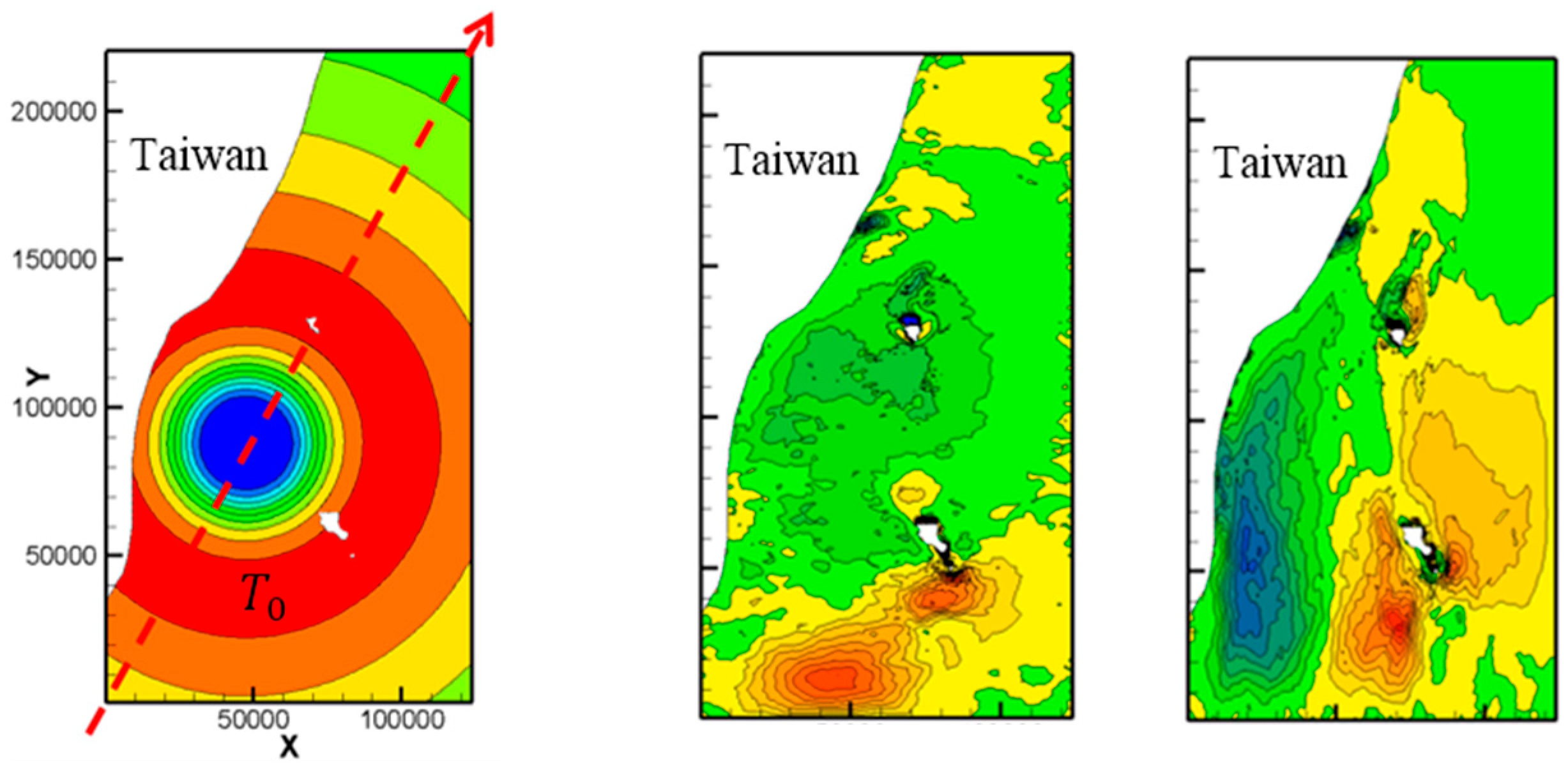

Figure 11.
Contours of (a) W10, “net” (b) u-, and (c) v-contours of (unit: m/s) SN typhoon with moving speed WT = 5.0 m/s at T0–T2 three time instances indicated by the three vertical lines of Figure 16b.
Figure 11.
Contours of (a) W10, “net” (b) u-, and (c) v-contours of (unit: m/s) SN typhoon with moving speed WT = 5.0 m/s at T0–T2 three time instances indicated by the three vertical lines of Figure 16b.


Figure 12.
(a) W10-contours and (b) wind vectors (red) and flow vectors (blue) of SN typhoon along cross section with moving speed WT = 2.5 m/s at T0–T2 three time instances indicated by the three vertical lines of Figure 16a.
Figure 12.
(a) W10-contours and (b) wind vectors (red) and flow vectors (blue) of SN typhoon along cross section with moving speed WT = 2.5 m/s at T0–T2 three time instances indicated by the three vertical lines of Figure 16a.


Figure 13.
Contours of (a) W10, “net” (b) u-, and (c) v-contours (unit: m/s) of EW typhoon with moving speed WT = 2.5 m/s at three time instances T0–T2 indicated by the three vertical lines of Figure 16a.
Figure 13.
Contours of (a) W10, “net” (b) u-, and (c) v-contours (unit: m/s) of EW typhoon with moving speed WT = 2.5 m/s at three time instances T0–T2 indicated by the three vertical lines of Figure 16a.
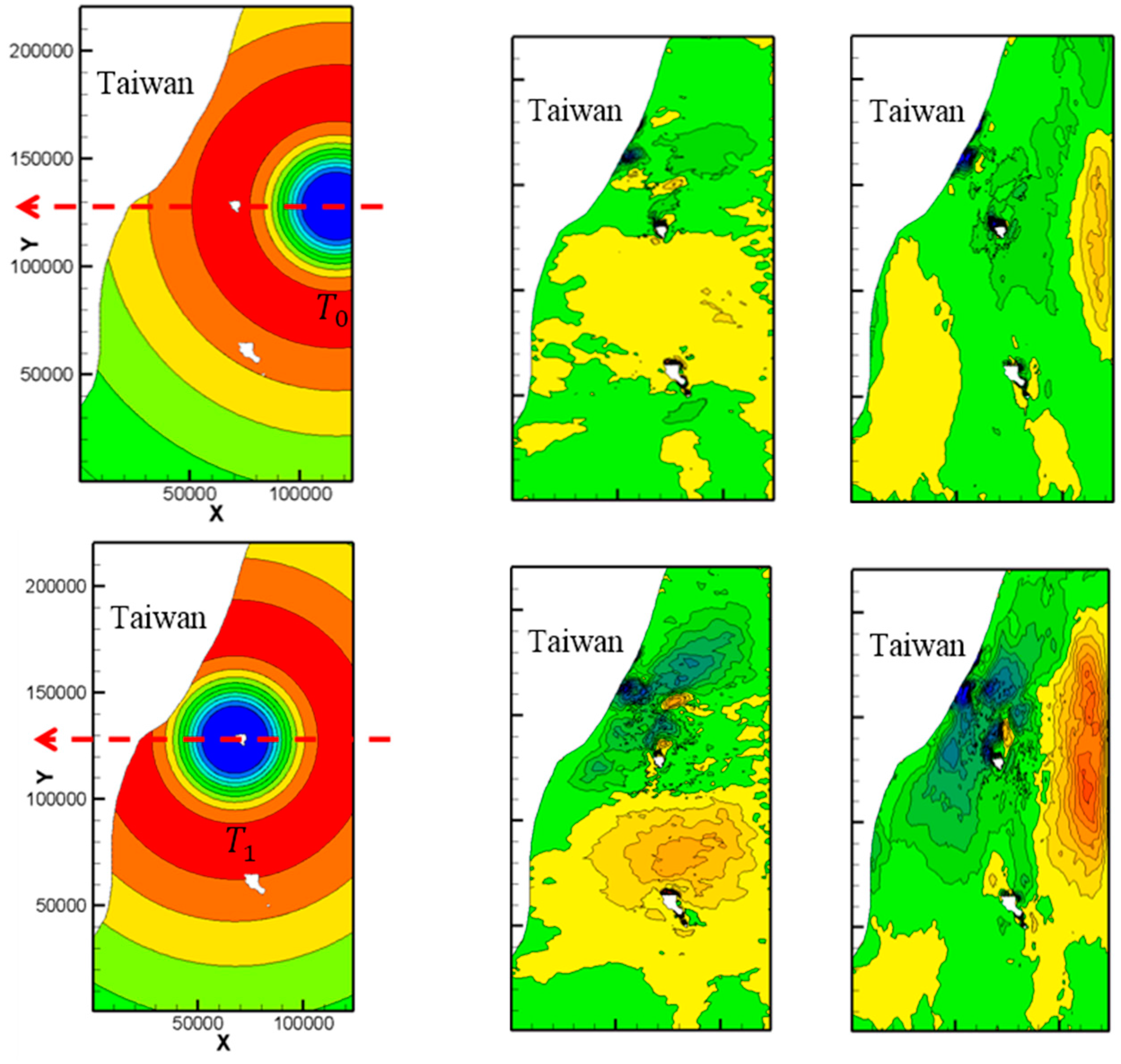

Figure 14.
Contours of (a) W10, “net”(b) u-, and (c) v-contours of (unit: m/s) EW typhoon with moving speed WT = 5.0 m/s at T0–T2 three time instances indicated by the three vertical lines of Figure 16b.
Figure 14.
Contours of (a) W10, “net”(b) u-, and (c) v-contours of (unit: m/s) EW typhoon with moving speed WT = 5.0 m/s at T0–T2 three time instances indicated by the three vertical lines of Figure 16b.
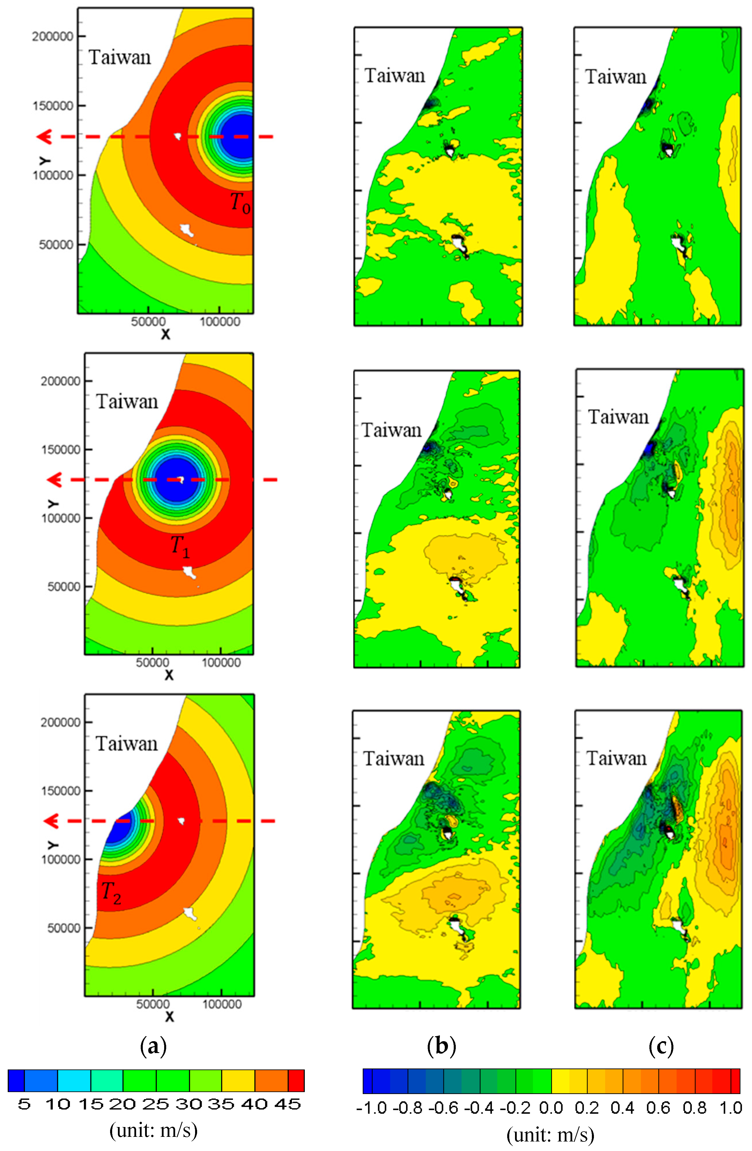
Figure 15.
(a) W10-contours and (b) wind vectors (red) and flow vectors (blue) of EW typhoon along cross section with moving speed WT = 2.5 m/s at T0–T2 three time instances indicated by the three vertical lines of Figure 16a.
Figure 15.
(a) W10-contours and (b) wind vectors (red) and flow vectors (blue) of EW typhoon along cross section with moving speed WT = 2.5 m/s at T0–T2 three time instances indicated by the three vertical lines of Figure 16a.
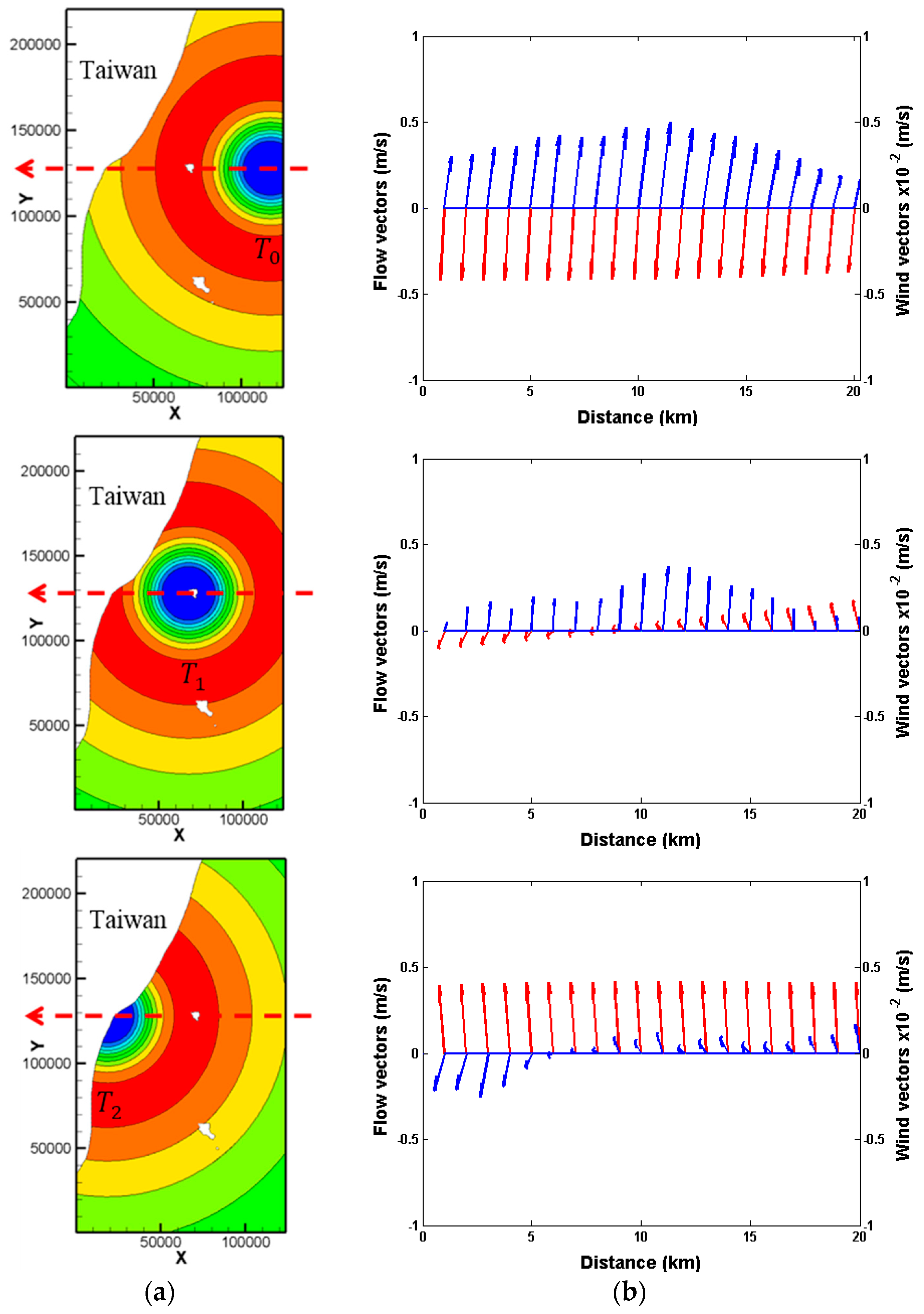
Figure 16.
Comparison of u and v of monitor point P of no wind, SN, and EW typhoon with the moving speed WT = (a) 2.5 m/s (upper row) and (b) 5.0 m/s (lower row), respectively.
Figure 16.
Comparison of u and v of monitor point P of no wind, SN, and EW typhoon with the moving speed WT = (a) 2.5 m/s (upper row) and (b) 5.0 m/s (lower row), respectively.
© 2018 by the authors. Licensee MDPI, Basel, Switzerland. This article is an open access article distributed under the terms and conditions of the Creative Commons Attribution (CC BY) license (http://creativecommons.org/licenses/by/4.0/).
Share and Cite
MDPI and ACS Style
Hsu, T.-W.; Chou, M.-H.; Chao, W.-T.; Liang, S.-J. Typhoon Effect on Kuroshio and Green Island Wakes: A Modelling Study. Atmosphere 2018, 9, 36. https://doi.org/10.3390/atmos9020036
AMA Style
Hsu T-W, Chou M-H, Chao W-T, Liang S-J. Typhoon Effect on Kuroshio and Green Island Wakes: A Modelling Study. Atmosphere. 2018; 9(2):36. https://doi.org/10.3390/atmos9020036
Chicago/Turabian StyleHsu, Tai-Wen, Meng-Hsien Chou, Wei-Ting Chao, and Shin-Jye Liang. 2018. "Typhoon Effect on Kuroshio and Green Island Wakes: A Modelling Study" Atmosphere 9, no. 2: 36. https://doi.org/10.3390/atmos9020036
Note that from the first issue of 2016, this journal uses article numbers instead of page numbers. See further details here.