Prediction of Wind Environment and Indoor/Outdoor Relationships for PM2.5 in Different Building–Tree Grouping Patterns


Abstract
:1. Introduction
2. Climate of Beijing
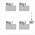
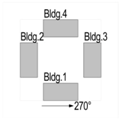
3. Simulation Case Descriptions
4. The CFD Code
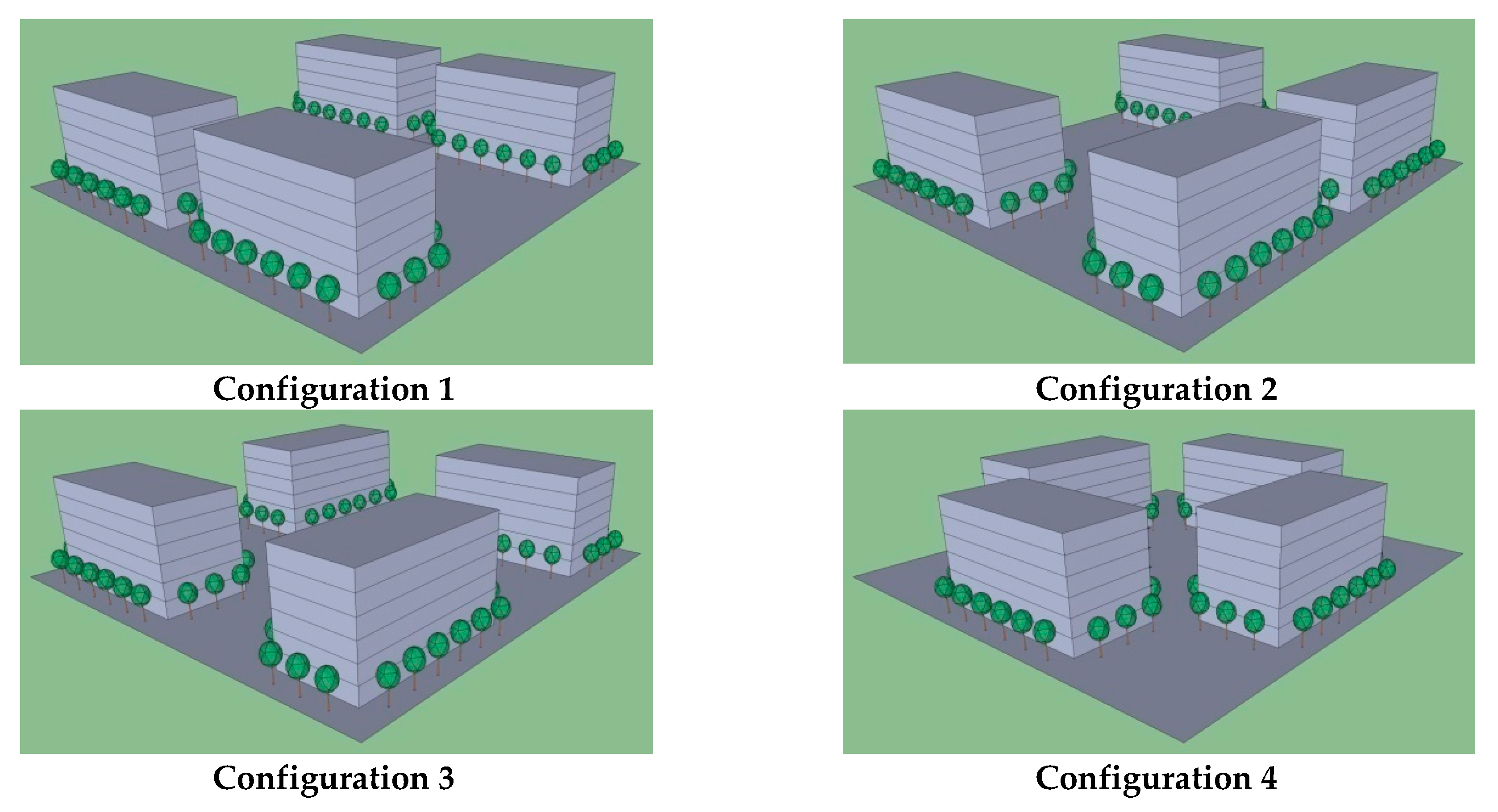
4.1. Simulation Models
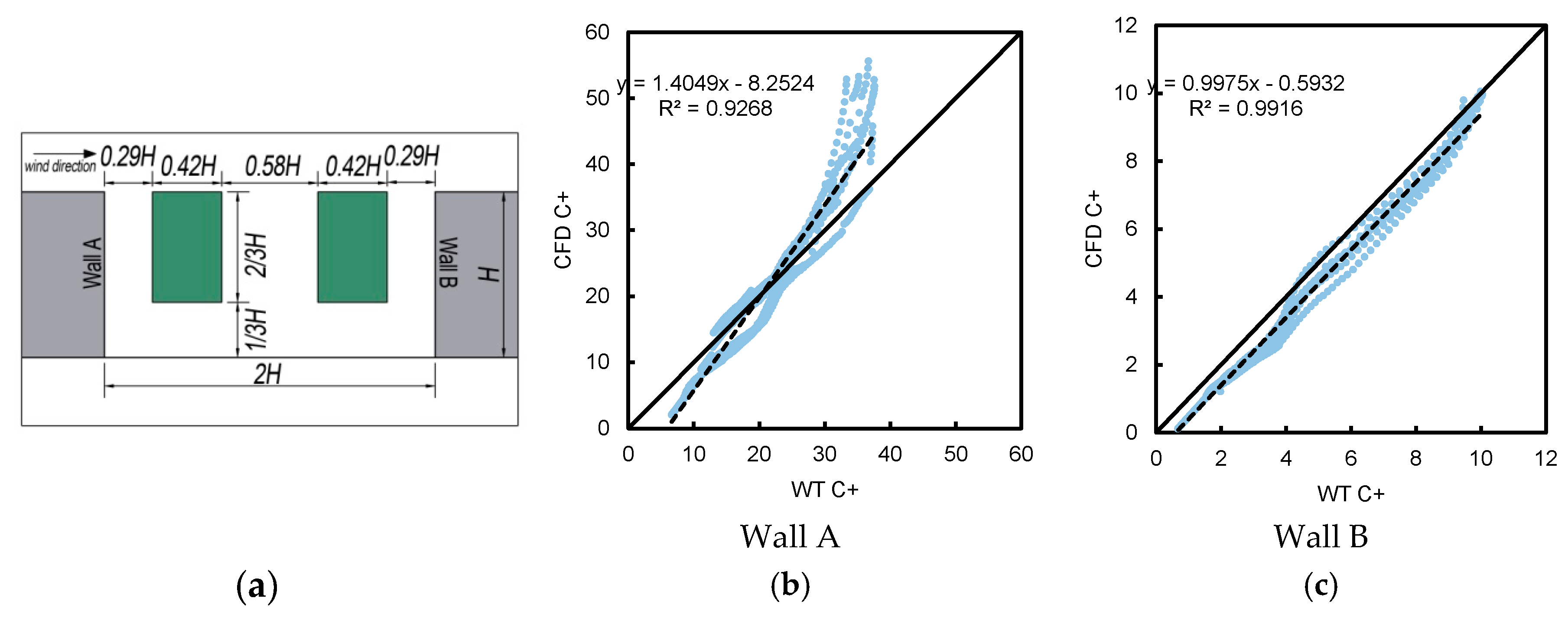
4.2. Model Validation
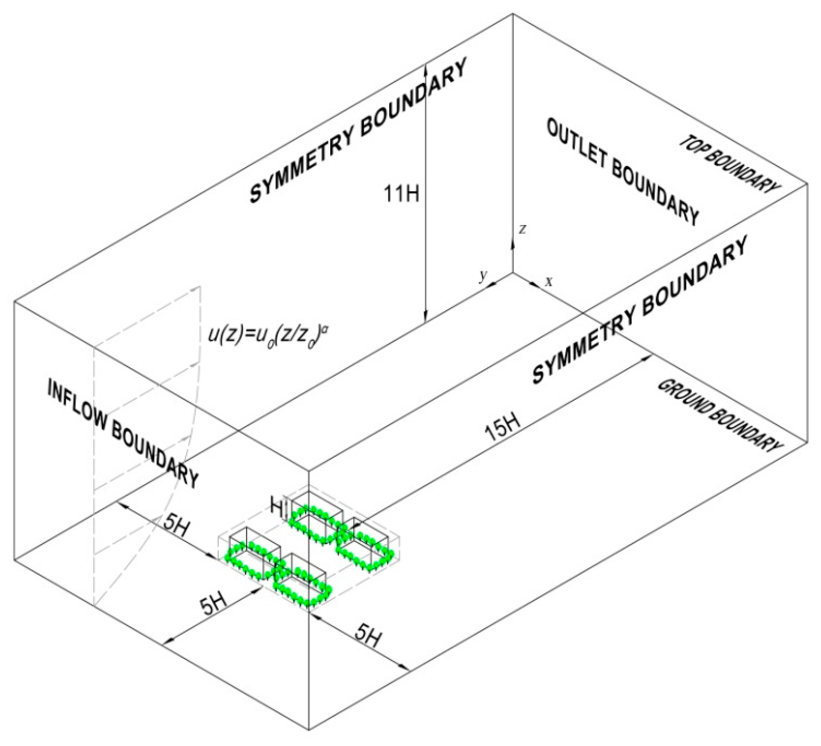
4.3. Domain Size and Grid Independence Testing
4.4. Boundary Conditions and Turbulence Model
4.5. Convergence Criteria
4.6. Simulation Target
- (1)
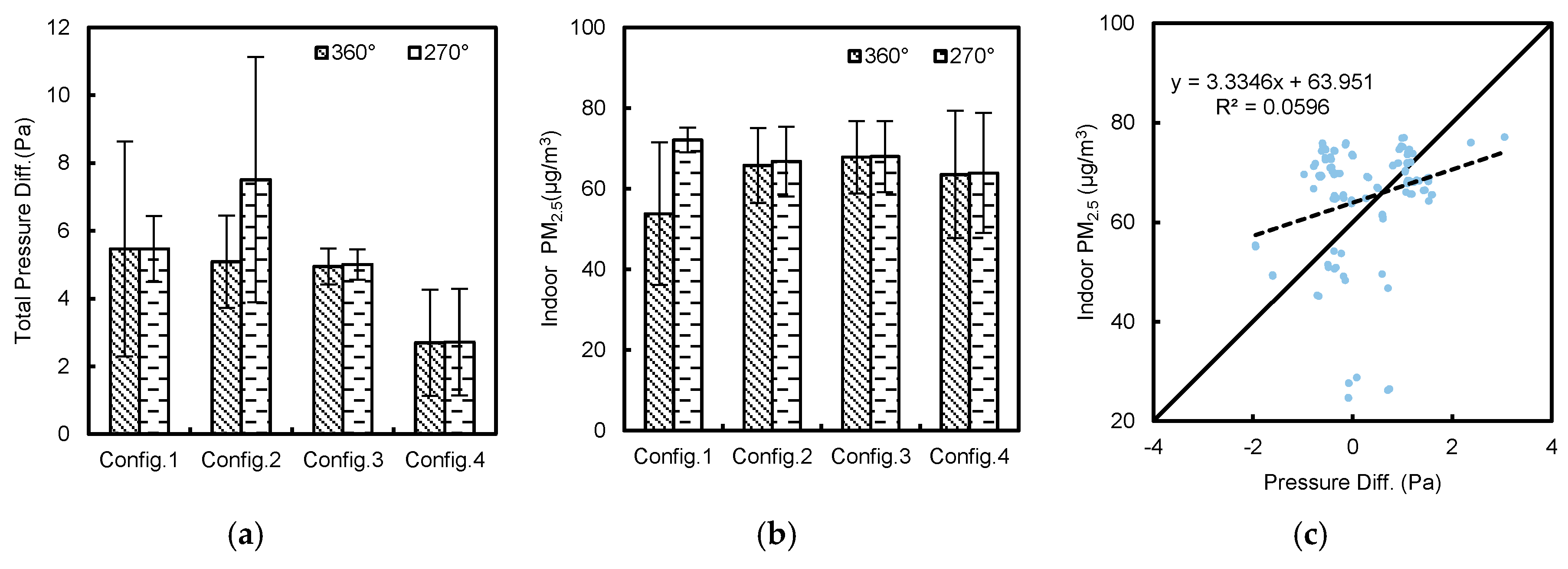
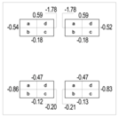
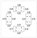
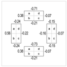
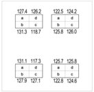
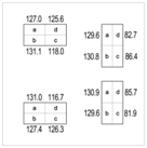
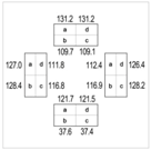
- Average wind pressure of each building façade was recorded.
- (2)
- (3)
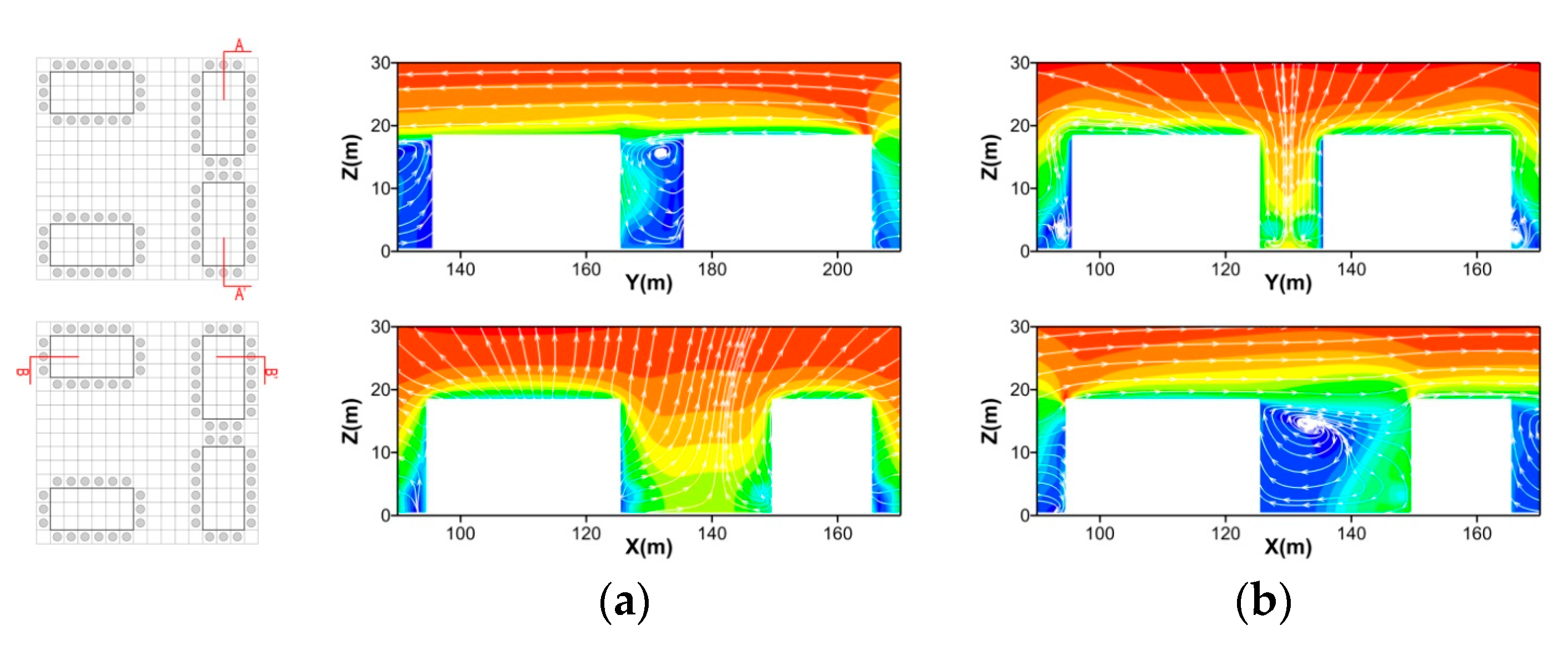
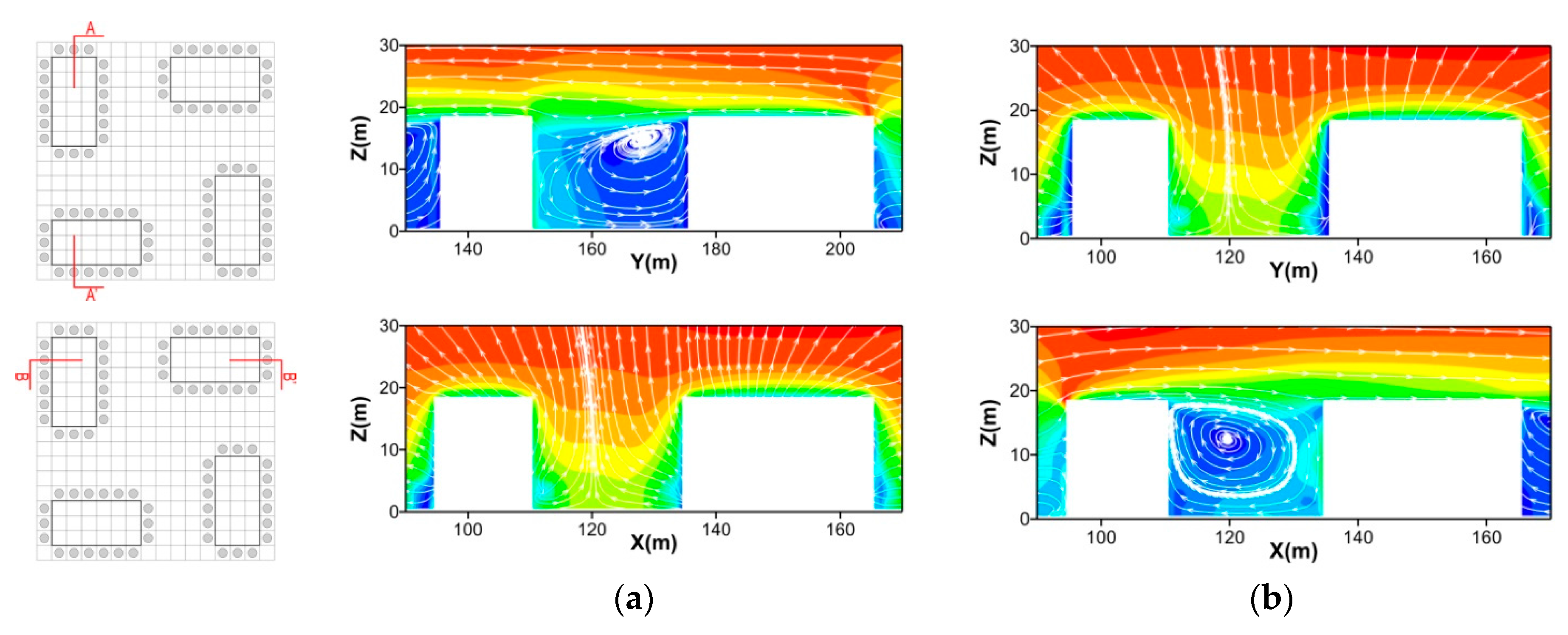
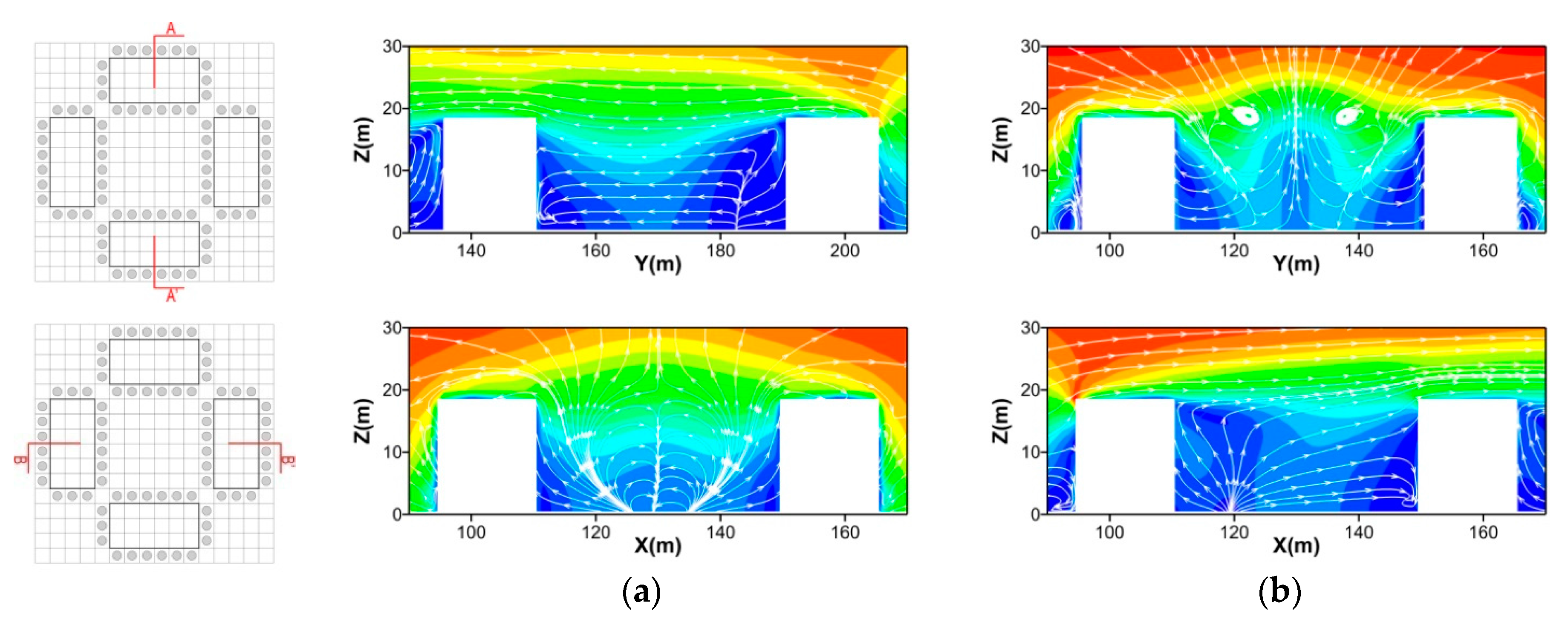
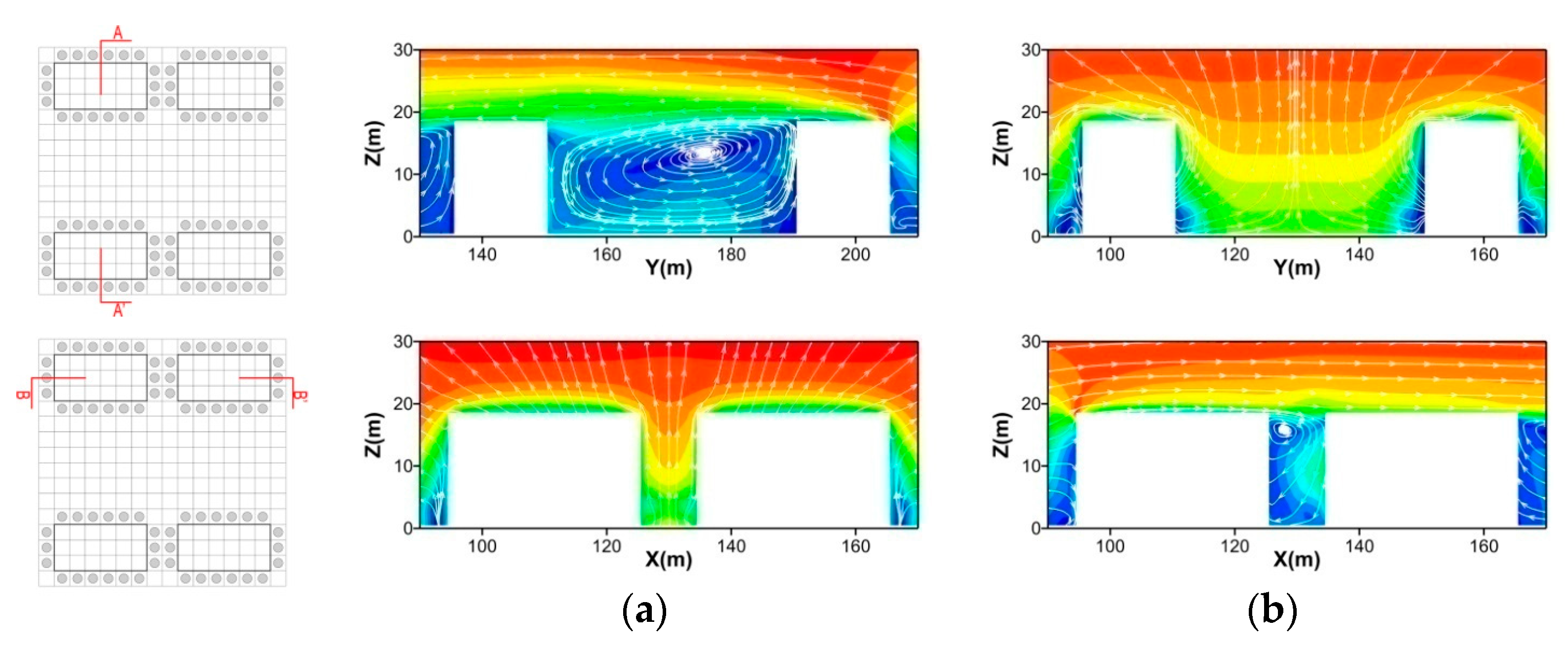
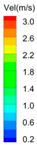
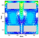
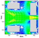
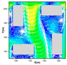
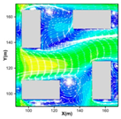
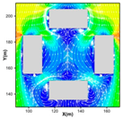
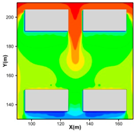
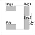
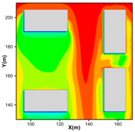
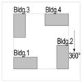
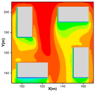
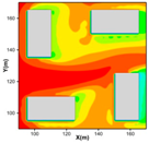
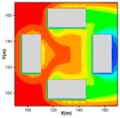
- Contours of wind velocity and streamlines at the pedestrian level, and contours of wind velocity and streamlines in sections A-A’ and B-B’ were also presented for better understanding the surrounding wind environment.
- (1)
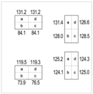
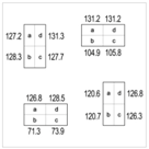
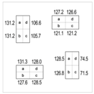
- Outdoor vertical PM2.5 concentrations were measured 0.5 m from the building facade. This was done for each of the four buildings.
- (2)
- Indoor concentrations across flats a to d in each building can be computed by Equation (12), as presented in Tables 7–10.
- (3)
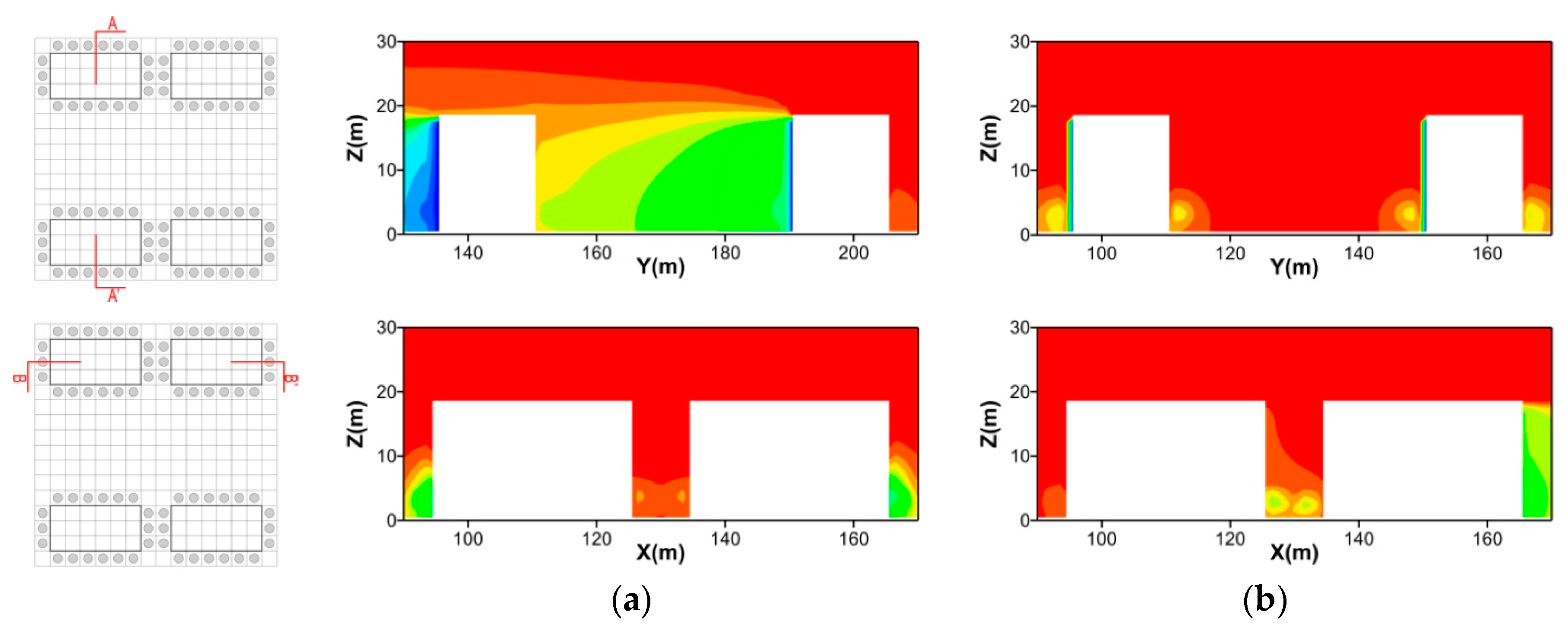
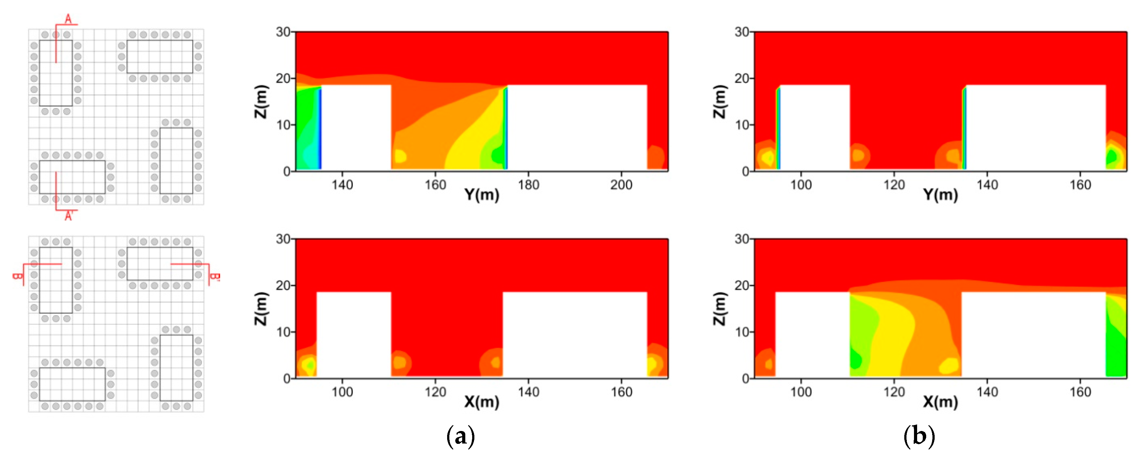
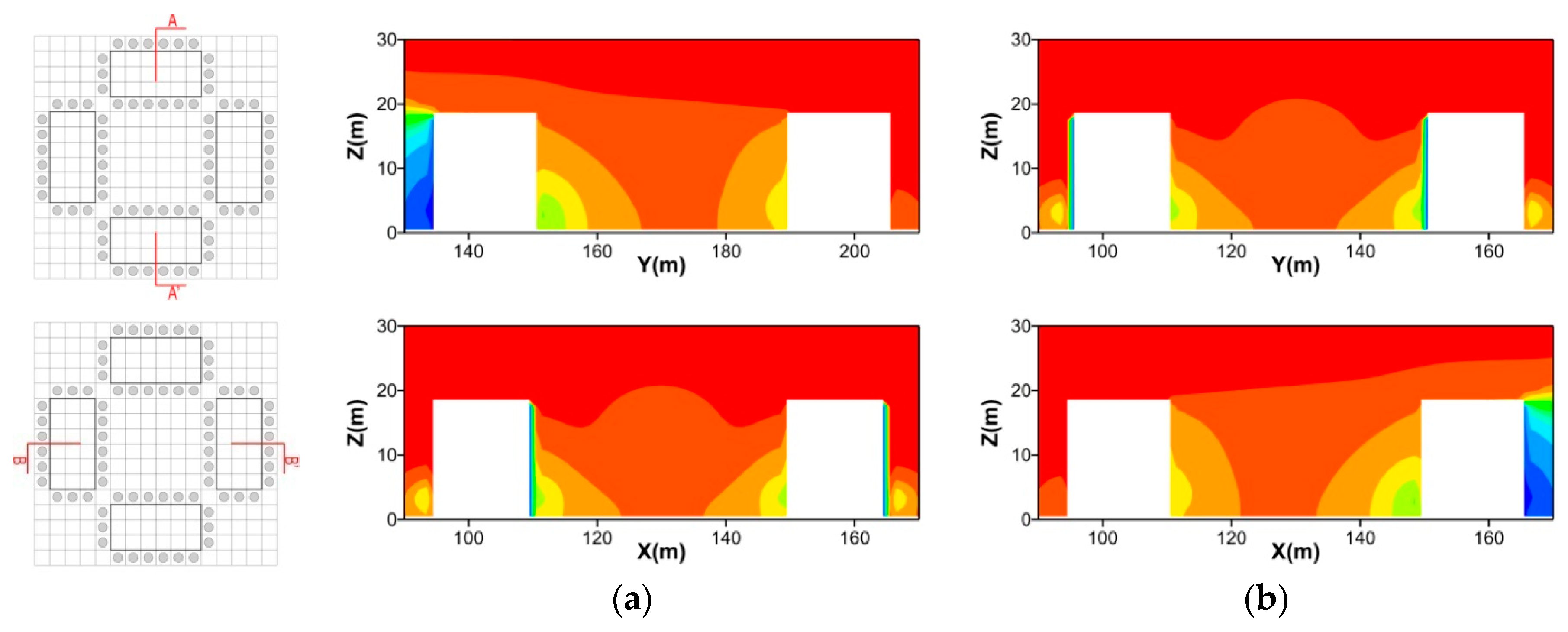
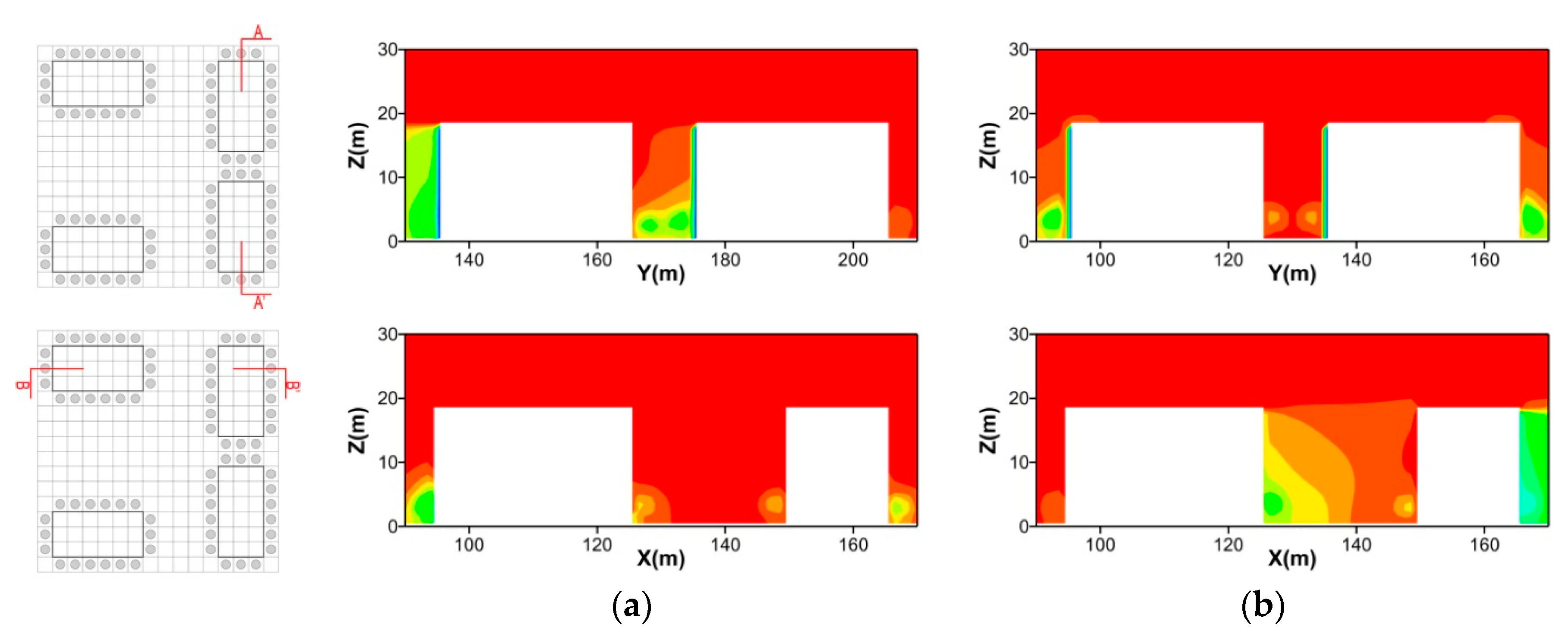
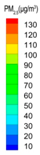
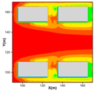
- Contours of pedestrian level PM2.5 concentrations, and PM2.5 dispersion in vertical level were also presented to understand the vertical PM2.5 concentrations (Figures 8–11).
5. Results and Discussion
5.1. Analysis of Outdoor Wind Environment
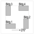
5.1.1. Configuration 1
5.1.2. Configuration 2
5.1.3. Configuration 3
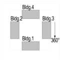
5.1.4. Configuration 4
5.2. Analysis of Indoor/Outdoor PM2.5
5.2.1. Configuration 1
5.2.2. Configuration 2
5.2.3. Configuration 3
5.2.4. Configuration 4
6. Conclusions
Acknowledgments
Author Contributions
Conflicts of Interest
References
- Brunekreef, B.; Holgate, S.T. Air pollution and health. Lancet 2002, 360, 1233–1242. [Google Scholar] [CrossRef]
- Zhang, X.; Zhang, X.; Chen, X. Happiness in the air: How does a dirty sky affect mental health and subjective well-being? J. Environ. Econ. Manag. 2017, 85, 81–94. [Google Scholar] [CrossRef] [PubMed]
- Abt, E.; Suh, H.H.; Catalano, P.; Koutrakis, P. Relative contribution of outdoor and indoor particle sources to indoor concentrations. Environ. Sci. Technol. 2000, 34, 3579–3587. [Google Scholar] [CrossRef]
- Ramachandran, G.; Adgate, J.L.; Pratt, G.C.; Sexton, K. Characterizing indoor and outdoor 15 minute average PM2.5 concentrations in urban neighborhoods. Aerosol Sci. Technol. 2003, 37, 33–45. [Google Scholar] [CrossRef]
- Schneider, T.; Jensen, K.A.; Clausen, P.A.; Afshari, A.; Gunnarsen, L.; Wåhlin, P.; Glasius, M.; Palmgren, F.; Nielsen, O.J.; Fogh, C.L. Prediction of indoor concentration of 0.5–4 μm particles of outdoor origin in an uninhabited apartment. Atmos. Environ. 2004, 38, 6349–6359. [Google Scholar] [CrossRef]
- Matson, U. Indoor and outdoor concentrations of ultrafine particles in some Scandinavian rural and urban areas. Sci. Total Environ. 2005, 343, 169–176. [Google Scholar] [CrossRef] [PubMed]
- Jones, A.P. Indoor air quality and health. Atmos. Environ. 1999, 33, 4535–4564. [Google Scholar] [CrossRef]
- Liao, C.M.; Huang, S.J.; Yu, H. Size-dependent particulate matter indoor/outdoor relationships for a wind-induced naturally ventilated airspace. Build. Environ. 2004, 39, 411–420. [Google Scholar] [CrossRef]
- De Jong, T.; Bot, G.P.A. Air exchange caused by wind effects through (window) openings distributed evenly on a quasi-infinite surface. Energy Build. 1992, 19, 93–103. [Google Scholar] [CrossRef]
- Miguel, A.F.; Van de Braak, N.J.; Silva, A.M.; Bot, G.P.A. Wind-induced airflow through permeable materials part I: Air infiltration in enclosure. J. Wind Eng. Ind. Aerodyn. 2001, 89, 59–72. [Google Scholar] [CrossRef]
- Tominaga, Y.; Mochida, A.; Shirasawa, T.; Yoshie, R.; Kataoka, H.; Harimoto, K.; Nozu, T. Cross comparisons of CFD results of wind environment at pedestrian level around a high-rise building and with a building complex. J. Asian Archit. Build. 2004, 3, 63–70. [Google Scholar] [CrossRef]
- Zhang, A.; Gao, C.; Zhang, L. Numerical simulation of the wind field around different building arrangements. J. Wind Eng. Ind. Aerodyn. 2005, 93, 891–904. [Google Scholar] [CrossRef]
- Asfour, O.S.; Gadi, M.B. A comparison between CFD and Network models for predicting wind-driven ventilation in buildings. Build. Environ. 2007, 42, 4079–4085. [Google Scholar] [CrossRef]
- Tominaga, Y.; Mochida, A.; Yoshie, R.; Kataoka, H.; Nozu, T.; Yoshikawa, M.; Shirasawa, T. AIJ guidelines for practical applications of CFD to pedestrian wind environment around buildings. J. Wind Eng. Ind. Aerodyn. 2008, 96, 1749–1761. [Google Scholar] [CrossRef]
- Kubota, T.; Miura, M.; Tominaga, Y.; Mochida, A. Wind tunnel tests on the relationship between building density and pedestrian-level wind velocity: Development of guidelines for realizing acceptable wind environment in residential neighborhoods. Build. Environ. 2008, 43, 1699–1708. [Google Scholar] [CrossRef]
- Mochida, A.; Lun, I.Y.F. Prediction of wind environment and thermal comfort at pedestrian level in urban area. J. Wind Eng. Ind. Aerodyn. 2008, 96, 1498–1527. [Google Scholar] [CrossRef]
- Asfour, O.S. Prediction of wind environment in different grouping patterns of housing blocks. Energy Build. 2010, 42, 2061–2069. [Google Scholar] [CrossRef]
- You, W.; Gao, Z.; Chen, Z.; Ding, W. Improving residential wind environments by understanding the relationship between building arrangements and outdoor regional ventilation. Atmosphere 2017, 8, 102. [Google Scholar] [CrossRef]
- Mochida, A.; Tabata, Y.; Iwata, T.; Yoshino, H. Examining tree canopy models for CFD prediction of wind environment at pedestrian level. J. Wind Eng. Ind. Aerodyn. 2008, 96, 1667–1677. [Google Scholar] [CrossRef]
- Chen, H.; Ooka, R.; Kato, S. Study on optimum design method for pleasant outdoor thermal environment using genetic algorithms (GA) and coupled simulation of convection, radiation and conduction. Build. Environ. 2008, 43, 18–30. [Google Scholar] [CrossRef]
- Hong, B.; Lin, B.; Hu, L.; Li, S. Optimal tree design for sunshine and ventilation in residential district using geometrical models and numerical simulation. Build. Simul. 2011, 4, 351–363. [Google Scholar] [CrossRef]
- Hong, B.; Lin, B.; Wang, B.; Li, S. Optimal design of vegetation in residential district with numerical simulation and field experiment. J. Cent. South Univ. 2012, 19, 688–695. [Google Scholar] [CrossRef]
- Hong, B.; Lin, B. Numerical studies of the outdoor wind environment and thermal comfort at pedestrian level in housing blocks with different building layout patterns and trees arrangement. Renew. Energy 2015, 73, 18–27. [Google Scholar] [CrossRef]
- Chen, C.; Zhao, B. Review of relationship between indoor and outdoor particles: I/O ratio, infiltration factor and penetration factor. Atmos. Environ. 2011, 45, 275–288. [Google Scholar] [CrossRef]
- Braniš, M.; Řezáčová, P.; Domasová, M. The effect of outdoor air and indoor human activity on mass concentrations of PM10, PM2.5, and PM1 in a classroom. Environ. Res. 2005, 99, 143–149. [Google Scholar] [CrossRef] [PubMed]
- Massey, D.; Masih, J.; Kulshrestha, A.; Habil, M.; Taneja, A. Indoor/outdoor relationship of fine particles less than 2.5 μm (PM2.5) in residential homes locations in central Indian region. Build. Environ. 2009, 44, 2037–2045. [Google Scholar] [CrossRef]
- Chithra, V.S.; Nagendra, S.M.S. Indoor air quality investigations in a naturally ventilated school building located close to an urban roadway in Chennai, India. Build. Environ. 2012, 54, 159–167. [Google Scholar] [CrossRef]
- Mohammadyan, M.; Ghoochani, M.; Kloog, I.; Abdul-Wahab, S.A.; Yetilmezsoy, K.; Heibati, B.; Pollitt, K.J.G. Assessment of indoor and outdoor particulate air pollution at an urban background site in Iran. Environ. Monit. Assess. 2017, 189, 235. [Google Scholar] [CrossRef] [PubMed]
- Hahn, I.; Brixey, L.A.; Wiener, R.W.; Henkle, S.W. Parameterization of meteorological variables in the process of infiltration of outdoor ultrafine particles into a residential building. J. Environ. Monit. 2009, 11, 2192–2200. [Google Scholar] [CrossRef] [PubMed]
- Chithra, V.S.; Nagendra, S.M.S. Impact of outdoor meteorology on indoor PM10, PM2.5 and PM1 concentrations in a naturally ventilated classroom. Urban Clim. 2014, 10, 77–91. [Google Scholar] [CrossRef]
- Riain, C.M.N.; Mark, D.; Davies, M.; Harrison, R.M.; Byrne, M.A. Averaging periods for indoor-outdoor ratios of pollution in naturally ventilated non-domestic buildings near a busy road. Atmos. Environ. 2003, 37, 4121–4132. [Google Scholar] [CrossRef]
- Massey, D.; Kulshrestha, A.; Masih, J.; Taneja, A. Seasonal trends of PM10, PM5.0, PM2.5& PM1.0 in indoor and outdoor environments of residential homes located in North-Central India. Build. Environ. 2012, 47, 223–231. [Google Scholar]
- Zhao, X.; Zhang, X.; Xu, X.; Xu, J.; Meng, W.; Pu, W. Seasonal and diurnal variations of ambient PM2.5 concentration in urban and rural environments in Beijing. Atmos. Environ. 2009, 43, 2893–2900. [Google Scholar] [CrossRef]
- Yang, F.; Kang, Y.; Gao, Y.; Zhong, K. Numerical simulations of the effect of outdoor pollutants on indoor air quality of buildings next to a street canyon. Build. Environ. 2015, 87, 10–22. [Google Scholar] [CrossRef]
- Zhao, B.; Zhang, Y.; Li, X.; Yang, X.; Huang, D. Comparison of indoor aerosol particle concentration and deposition in different ventilated rooms by numerical method. Build. Environ. 2004, 39, 1–8. [Google Scholar] [CrossRef]
- Quang, T.N.; He, C.; Morawska, L.; Knibbs, L.D. Influence of ventilation and filtration on indoor particle concentrations in urban office buildings. Atmos. Environ. 2013, 79, 41–52. [Google Scholar] [CrossRef]
- Kopperud, R.J.; Ferro, A.R.; Hildemann, L.M. Outdoor versus indoor contributions to indoor particulate matter (PM) determined by mass balance methods. J. Air Waste Manag. Assoc. 2004, 54, 1188–1196. [Google Scholar] [CrossRef] [PubMed]
- Zhao, L.; Chen, C.; Wang, P.; Chen, Z.; Cao, S.; Wang, Q.; Xie, G.; Wan, Y.; Wang, Y.; Lu, B. Influence of atmospheric fine particulate matter (PM2.5) pollution on indoor environment during winter in Beijing. Build. Environ. 2015, 87, 283–291. [Google Scholar] [CrossRef]
- Hussein, T. Indoor-to-outdoor relationship of aerosol particles inside a naturally ventilated apartment-A comparison between single-parameter analysis and indoor aerosol model simulation. Sci. Total Environ. 2017, 596, 321–330. [Google Scholar] [CrossRef] [PubMed]
- Bo, M.; Salizzoni, P.; Clerico, M.; Buccolieri, R. Assessment of Indoor-Outdoor Particulate Matter Air Pollution: A Review. Atmosphere 2017, 8, 136. [Google Scholar] [CrossRef]
- Hong, B.; Lin, B.; Qin, H. Numerical investigation on the coupled effects of building-tree arrangements on fine particulate matter (PM2.5) dispersion in housing blocks. Sustain. Cities Soc. 2017, 34, 358–370. [Google Scholar] [CrossRef]
- Building Energy Conservation Research Center, Tsinghua University (BECRC). Annual Report on Chinese Building Energy Conservation Development 2016; China Architecture & Building Press: Beijing, China, 2016. [Google Scholar]
- Shi, S.; Zhao, B. Occupants’ interactions with windows in 8 residential apartments in Beijing and Nanjing, China. Build. Simul. 2016, 9, 221–231. [Google Scholar] [CrossRef]
- Ye, B.; Ji, X.; Yang, H.; Yao, X.; Chan, C.K.; Cadle, S.H.; Chan, T.; Mulawa, P.A. Concentration and chemical composition of PM2.5 in Shanghai for a 1-year period. Atmos. Environ. 2003, 37, 499–510. [Google Scholar] [CrossRef]
- Beijing Municipal Environmental Monitoring Center (BMEMC). Real-Time Air Quality in Beijing. Available online: http://www.bjmemc.com.cn (accessed on 1 January 2016).
- World Health Organization (WHO). WHO Air Quality Guidelines for Particulate Matter, Ozone, Nitrogen Dioxide and Sulfur Dioxide. Available online: http://apps.who.int/iris/bitstream/10665/69477/1/WHO_SDE_PHE_OEH_06.02_eng.pdf (accessed on 2 June 2005).
- Freer-Smith, P.H.; Beckett, K.P.; Taylor, G. Deposition velocities to Sorbus aria, Acer campestre, Populus deltoids×trichocarpa ‘Beaupré’, Pinus nigra and× Cupressocyparis leylandii for coarse, fine and ultra-fine particles in the urban environment. Environ. Pollut. 2005, 133, 157–167. [Google Scholar] [CrossRef] [PubMed]
- Franke, J.; Hellsten, A.; Schlunzen, K.H.; Carissimo, B. The COST 732 best practice guideline for CFD simulation of flows in the urban environment: A summary. Int. J. Environ. Pollut. 2011, 44, 419–427. [Google Scholar] [CrossRef]
- Lin, B.; Li, X.; Zhu, Y.; Qin, Y. Numerical simulation studies of the different vegetation patterns’ effects on outdoor pedestrian thermal comfort. J. Wind Eng. Ind. Aerodyn. 2008, 96, 1707–1718. [Google Scholar] [CrossRef]
- Finnigan, J. Turbulence in plant canopies. Annu. Rev. Fluid Mech. 2000, 32, 519–571. [Google Scholar] [CrossRef]
- Sanz, C. A note on k-epsilon modelling of vegetation canopy air-flows. Bound.-Layer Meteorol. 2003, 108, 191–197. [Google Scholar] [CrossRef]
- Katul, G.G.; Mahrt, L.; Poggi, D.; Sanz, C. One-and two-equation models for canopy turbulence. Bound.-Layer Meteorol. 2004, 113, 81–109. [Google Scholar] [CrossRef]
- Endalew, A.M.; Hertog, M.; Delele, M.A.; Baetens, K.; Persoons, T.; Baelmans, M.; Ramon, H.; Nicolai, B.M.; Verboven, P. CFD modelling and wind tunnel validation of airflow through plant canopies using 3D canopy architecture. Int. J. Heat Fluid Flow 2009, 30, 356–368. [Google Scholar] [CrossRef]
- Ji, W.; Zhao, B. Numerical study of the effects of trees on outdoor particle concentration distributions. Build. Simul. 2014, 7, 417–427. [Google Scholar] [CrossRef]
- Vranckx, S.; Vos, P.; Maiheu, B.; Janssen, S. Impact of trees on pollutant dispersion in street canyons: A numerical study of the annual average effects in Antwerp, Belgium. Sci. Total Environ. 2015, 532, 474–483. [Google Scholar] [CrossRef] [PubMed]
- Jeanjean, A.P.R.; Monks, P.S.; Leigh, R.J. Modelling the effectiveness of urban trees and grass on PM2.5 reduction via dispersion and deposition at a city scale. Atmos. Environ. 2016, 147, 1–10. [Google Scholar] [CrossRef]
- Santiago, J.L.; Martilli, A.; Martin, F. On dry deposition modelling of atmospheric pollutants on vegetation at the microscale: Application to the impact of street vegetation on air quality. Bound.-Layer Meteorol. 2016, 162, 1–24. [Google Scholar] [CrossRef]
- Bell, J.N.B.; Treshow, M. (Eds.) Air Pollution and Plant Life, 2nd ed.; John Willey & Sons Ltd.: Chichester, UK, 2003. [Google Scholar]
- Concentration Data of Street Canyons (CODASC). Available online: http://www.windforschung.de/CODASC.htm (accessed on 1 January 2008).
- Gromke, C.; Blocken, B. Influence of avenue-trees on air quality at the urban neighborhood scale. Part I: Quality assurance studies and turbulent Schmidt number analysis for RANS CFD simulations. Environ. Pollut. 2015, 196, 214–223. [Google Scholar] [CrossRef] [PubMed]
- Roache, P.J. Perspective: A method for uniform reporting of grid refinement studies. J. Fluids Eng. 1994, 116, 405–413. [Google Scholar] [CrossRef]
- Gromke, C.; Ruck, B. Pollutant concentrations in street canyons of different aspect ratio with avenues of trees for various wind directions. Bound.-Layer Meteorol. 2012, 144, 41–64. [Google Scholar] [CrossRef]
- Hanna, S.; Chang, J. Acceptance criteria for urban dispersion model evaluation. Meteorol. Atmos. Phys. 2012, 116, 133–146. [Google Scholar] [CrossRef]
- Hong, B.; Lin, B.; Qin, H. Numerical investigation on the effect of avenue trees on PM2.5 dispersion in urban street canyons. Atmosphere 2017, 8, 129. [Google Scholar] [CrossRef]
- Hefny, M.M.; Ooka, R. CFD analysis of pollutant dispersion around buildings: Effect of cell geometry. Build. Environ. 2009, 44, 1699–1706. [Google Scholar] [CrossRef]
- Barratt, R. Atmospheric Dispersion Modeling: An Introduction to Practical Applications; Earthscan: London, UK, 2001. [Google Scholar]
- Jin, R.; Hang, J.; Liu, S.; Wei, J.; Liu, Y.; Xie, J.; Sandberg, M. Numerical investigation of wind-driven natural ventilation performance in a multi-storey hospital by coupling indoor and outdoor airflow. Indoor Built Environ. 2016, 25, 1226–1247. [Google Scholar] [CrossRef]
- Lee, B.H.; Yee, S.W.; Kang, D.H.; Yeo, M.S.; Kim, K.W. Multi-zone simulation of outdoor particle penetration and transport in a multi-storey building. Build. Simul. 2017, 10, 525–534. [Google Scholar] [CrossRef]
- King, M.; Gough, H.L.; Halios, C.; Barlow, J.F.; Robertson, A.; Hoxey, R.; Noakes, C.J. Investigating the influence of neighbouring structures on natural ventilation potential of a full-scale cubical building using time-dependent CFD. J. Wind Eng. Ind. Aerodyn. 2017, 169, 265–279. [Google Scholar] [CrossRef]
- Chan, A.T. Indoor–outdoor relationships of particulate matter and nitrogen oxides under different outdoor meteorological conditions. Atmos. Environ. 2002, 36, 1543–1551. [Google Scholar] [CrossRef]


| Wall | Mean Concentration* | Statistical Analysis Metrics | ||||||
|---|---|---|---|---|---|---|---|---|
| WT C+ | CFD C+ | RD | FB | NMSE | FAC2 | NAD | R | |
| A | 20.77 | 20.92 | 6.6% | −0.007 | 0.052 | 1.008 | 0.083 | 0.961 |
| B | 3.90 | 3.30 | −15.4% | 0.1674 | 0.033 | 0.846 | 0.084 | 0.994 |
| Mesh | Minimum Grid Dimension | Total Cellnumber |
|---|---|---|
| coarse mesh | Xmin = Ymin = Zmin = 0.1H | 1,566,234 |
| fine mesh | Xmin = Ymin = Zmin = 0.05H | 3,001,458 |
| finest mesh | Xmin = Ymin = Zmin = 0.02H | 5,863,544 |
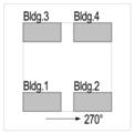
| V | Case | V Contours at 1.5 m | Pav. (Pa) | dP across Flats a to d (Pa) | ||||
|---|---|---|---|---|---|---|---|---|
 |  |  |  | Block No. | ||||
| Bldg.1 | Bldg.2 | Bldg.3 | Bldg.4 | |||||
| a | −0.39 | 0.26 | 1.13 | 2.37 | ||||
| b | 0.74 | 0.08 | −0.37 | −1.60 | ||||
| c | 0.08 | 0.70 | −1.16 | −0.34 | ||||
| d | 0.27 | −0.36 | 2.38 | 1.10 | ||||
 |  | 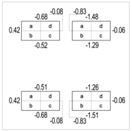 | Block No. | |||||
| Bldg.1 | Bldg.2 | Bldg.3 | Bldg.4 | |||||
| a | 0.93 | −0.43 | 1.10 | −0.65 | ||||
| b | 1.11 | −0.68 | 0.95 | −0.45 | ||||
| c | −0.61 | 1.45 | −0.45 | 1.23 | ||||
| d | −0.43 | 1.19 | −0.60 | 1.42 | ||||
| V | Case | V Contours at 1.5 m | Pav. (Pa) | dP across Flats a to d (Pa) | ||||
|---|---|---|---|---|---|---|---|---|
| |  |  |  | Block No. | ||||
| Bldg.1 | Bldg.2 | Bldg.3 | Bldg.4 | |||||
| a | −0.38 | −0.34 | 1.14 | 1.52 | ||||
| b | 0.71 | 1.07 | −0.38 | −0.98 | ||||
| c | 0.59 | 1.52 | −0.23 | −0.63 | ||||
| d | −0.26 | −0.79 | 0.99 | 1.16 | ||||
 |  |  | Block No. | |||||
| Bldg.1 | Bldg.2 | Bldg.3 | Bldg.4 | |||||
| a | 0.90 | 3.05 | 1.05 | 1.59 | ||||
| b | 1.06 | 1.58 | 0.92 | 3.05 | ||||
| c | −0.55 | −0.49 | −0.41 | −1.95 | ||||
| d | −0.40 | −1.95 | −0.55 | −0.50 | ||||
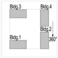
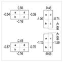
| V | Case | V Contours at 1.5 m | Pav. (Pa) | dP across Flats a to d (Pa) | ||||
|---|---|---|---|---|---|---|---|---|
| |  |  |  | Block No. | ||||
| Bldg.1 | Bldg.2 | Bldg.3 | Bldg.4 | |||||
| a | 1.51 | −0.38 | 1.09 | 1.03 | ||||
| b | −0.68 | 0.49 | −0.54 | −0.18 | ||||
| c | −0.15 | 1.15 | −0.78 | −0.33 | ||||
| d | 0.97 | 0.29 | 1.33 | 1.18 | ||||
 |  |  | Block No. | |||||
| Bldg.1 | Bldg.2 | Bldg.3 | Bldg.4 | |||||
| a | 1.29 | 1.00 | 1.21 | 0.31 | ||||
| b | 1.09 | 1.53 | 1.03 | −0.36 | ||||
| c | −0.55 | −0.71 | −0.19 | 0.51 | ||||
| d | −0.75 | −0.19 | −0.37 | 1.18 | ||||
| V | Case | V Contours at 1.5 m | Pav. (Pa) | dP across Flats a to d (Pa) | ||||
|---|---|---|---|---|---|---|---|---|
| |  |  |  | Block No. | ||||
| Bldg.1 | Bldg.2 | Bldg.3 | Bldg.4 | |||||
| a | −0.02 | 1.09 | 0.60 | 0.81 | ||||
| b | −0.09 | −0.63 | −0.14 | −0.03 | ||||
| c | −0.09 | −0.15 | −0.63 | −0.02 | ||||
| d | −0.01 | 0.61 | 1.09 | 0.81 | ||||
 |  |  | Block No. | |||||
| Bldg.1 | Bldg.2 | Bldg.3 | Bldg.4 | |||||
| a | 0.59 | 0.80 | 0.01 | 1.09 | ||||
| b | 1.11 | 0.81 | 0.01 | 0.59 | ||||
| c | −0.66 | −0.03 | −0.08 | −0.14 | ||||
| d | −0.14 | −0.02 | −0.08 | −0.64 | ||||
| C | Case | C Contours at 1.5 m | Outdoor Vertical Cav. (μg/m3) | Indoor Cav. across Flats a to d (μg/m3) | ||||
|---|---|---|---|---|---|---|---|---|
 |  |  |  | Block No. | ||||
| Bldg.1 | Bldg.2 | Bldg.3 | Bldg.4 | |||||
| a | 64.7 | 64.8 | 68.4 | 76.0 | ||||
| b | 26.5 | 28.7 | 50.6 | 49.2 | ||||
| c | 28.8 | 26.2 | 49.4 | 50.9 | ||||
| d | 64.8 | 64.6 | 76.0 | 68.4 | ||||
 |  |  | Block No. | |||||
| Bldg.1 | Bldg.2 | Bldg.3 | Bldg.4 | |||||
| a | 74.7 | 71.1 | 73.6 | 69.5 | ||||
| b | 75.9 | 69.4 | 74.8 | 70.9 | ||||
| c | 74.1 | 66.5 | 73.1 | 68.1 | ||||
| d | 72.6 | 68.1 | 75.3 | 66.4 | ||||
| C | Case | C Contours at 1.5 m | Outdoor Vertical Cav. (μg/m3) | Indoor Cav. across Flats a to d (μg/m3) | ||||
|---|---|---|---|---|---|---|---|---|
| |  |  |  | Block No. | ||||
| Bldg.1 | Bldg.2 | Bldg.3 | Bldg.4 | |||||
| a | 69.6 | 69.8 | 74.6 | 68.2 | ||||
| b | 46.7 | 66.0 | 54.2 | 69.6 | ||||
| c | 49.6 | 64.3 | 53.7 | 74.3 | ||||
| d | 69.8 | 66.8 | 76.9 | 72.1 | ||||
 |  |  | Block No. | |||||
| Bldg.1 | Bldg.2 | Bldg.3 | Bldg.4 | |||||
| a | 71.8 | 77.1 | 70.1 | 65.5 | ||||
| b | 73.0 | 65.5 | 71.9 | 77.1 | ||||
| c | 70.4 | 50.9 | 70.3 | 55.4 | ||||
| d | 70.1 | 55.1 | 72.6 | 51.5 | ||||
| C | Case | C Contours at 1.5 m | Outdoor Vertical Cav. (μg/m3) | Indoor Cav. across Flats a to d (μg/m3) | ||||
|---|---|---|---|---|---|---|---|---|
| |  |  |  | Block No. | ||||
| Bldg.1 | Bldg.2 | Bldg.3 | Bldg.4 | |||||
| a | 68.9 | 74.4 | 71.7 | 77.0 | ||||
| b | 45.1 | 67.0 | 74.5 | 64.8 | ||||
| c | 48.3 | 65.7 | 71.2 | 64.9 | ||||
| d | 75.3 | 69.2 | 68.3 | 73.8 | ||||
 |  |  | Block No. | |||||
| Bldg.1 | Bldg.2 | Bldg.3 | Bldg.4 | |||||
| a | 68.5 | 75.1 | 73.8 | 69.0 | ||||
| b | 71.9 | 69.0 | 77.0 | 74.3 | ||||
| c | 74.7 | 45.3 | 65.5 | 66.8 | ||||
| d | 71.8 | 49.1 | 65.4 | 65.7 | ||||
| C | Case | C Contours at 1.5 m | Outdoor Vertical Cav. (μg/m3) | Indoor Cav. across Flats a to d (μg/m3) | ||||
|---|---|---|---|---|---|---|---|---|
| |  |  |  | Block No. | ||||
| Bldg.1 | Bldg.2 | Bldg.3 | Bldg.4 | |||||
| a | 73.6 | 68.1 | 61.1 | 71.4 | ||||
| b | 24.7 | 69.4 | 75.8 | 64.4 | ||||
| c | 24.6 | 75.6 | 69.3 | 64.2 | ||||
| d | 73.6 | 60.7 | 67.8 | 71.4 | ||||
 |  |  | Block No. | |||||
| Bldg.1 | Bldg.2 | Bldg.3 | Bldg.4 | |||||
| a | 61.2 | 71.4 | 73.3 | 67.7 | ||||
| b | 68.0 | 71.4 | 73.3 | 61.5 | ||||
| c | 69.1 | 64.1 | 27.6 | 75.9 | ||||
| d | 75.9 | 63.7 | 27.6 | 69.1 | ||||
© 2018 by the authors. Licensee MDPI, Basel, Switzerland. This article is an open access article distributed under the terms and conditions of the Creative Commons Attribution (CC BY) license (http://creativecommons.org/licenses/by/4.0/).
Share and Cite
Hong, B.; Qin, H.; Lin, B. Prediction of Wind Environment and Indoor/Outdoor Relationships for PM2.5 in Different Building–Tree Grouping Patterns. Atmosphere 2018, 9, 39. https://doi.org/10.3390/atmos9020039
Hong B, Qin H, Lin B. Prediction of Wind Environment and Indoor/Outdoor Relationships for PM2.5 in Different Building–Tree Grouping Patterns. Atmosphere. 2018; 9(2):39. https://doi.org/10.3390/atmos9020039
Chicago/Turabian StyleHong, Bo, Hongqiao Qin, and Borong Lin. 2018. "Prediction of Wind Environment and Indoor/Outdoor Relationships for PM2.5 in Different Building–Tree Grouping Patterns" Atmosphere 9, no. 2: 39. https://doi.org/10.3390/atmos9020039