On the Increasing Importance of Air-Sea Exchanges in a Thawing Arctic: A Review


1
NASA Langley Research Center, Hampton, VA 23606, USA
2
Science Systems Applications Inc., Hampton, VA 23666, USA
3
Earth System Science Interdisciplinary Center, College Park, MD 20740, USA
*
Author to whom correspondence should be addressed.
Atmosphere 2018, 9(2), 41; https://doi.org/10.3390/atmos9020041
Submission received: 20 October 2017
/
Revised: 17 January 2018
/
Accepted: 19 January 2018
/
Published: 26 January 2018
(This article belongs to the Special Issue Air-Sea Coupling)
Abstract
:Forty years ago, climate scientists predicted the Arctic to be one of Earth’s most sensitive climate regions and thus extremely vulnerable to increased CO2. The rapid and unprecedented changes observed in the Arctic confirm this prediction. Especially significant, observed sea ice loss is altering the exchange of mass, energy, and momentum between the Arctic Ocean and atmosphere. As an important component of air–sea exchange, surface turbulent fluxes are controlled by vertical gradients of temperature and humidity between the surface and atmosphere, wind speed, and surface roughness, indicating that they respond to other forcing mechanisms such as atmospheric advection, ocean mixing, and radiative flux changes. The exchange of energy between the atmosphere and surface via surface turbulent fluxes in turn feeds back on the Arctic surface energy budget, sea ice, clouds, boundary layer temperature and humidity, and atmospheric and oceanic circulations. Understanding and attributing variability and trends in surface turbulent fluxes is important because they influence the magnitude of Arctic climate change, sea ice cover variability, and the atmospheric circulation response to increased CO2. This paper reviews current knowledge of Arctic Ocean surface turbulent fluxes and their effects on climate. We conclude that Arctic Ocean surface turbulent fluxes are having an increasingly consequential influence on Arctic climate variability in response to strong regional trends in the air-surface temperature contrast related to the changing character of the Arctic sea ice cover. Arctic Ocean surface turbulent energy exchanges are not smooth and steady but rather irregular and episodic, and consideration of the episodic nature of surface turbulent fluxes is essential for improving Arctic climate projections.
1. Introduction
The atmosphere can extract immense power from the ocean via air–sea energy exchanges. These exchanges drive global weather systems on scales ranging from individual thunderstorms to global circulation patterns [1,2,3,4], including polar lows containing hurricane-force winds exceeding 25 m s−1 [5]. Representing a primary conduit for atmosphere-ocean communication, air–sea interactions serve as the linchpin connecting the Earth’s ocean and atmosphere [6,7]. Uncertainty remains in our ability to simulate mean values and variability in all Arctic Ocean air–sea fluxes, especially within climate models, inhibiting our ability to make Arctic climate change projections and determine how the Arctic interacts with global weather and climate [7,8].
Arctic air–sea exchange comes in many forms including fluxes of mass (water vapor, gases, and aerosol), energy (surface turbulent and radiative fluxes), and momentum that modulate global and Arctic climate variability [7,9]. These radiative and surface turbulent air–sea exchanges compose the surface energy budget and control surface temperature and water phase transition. Changes in surface temperature and the surface energy budget are considered to be forced by large-scale atmospheric variability affecting the temperature and humidity profile and winds, as well as surface radiative fluxes [7,10,11]. Determined by near-surface vertical gradients of temperature and humidity between the surface and atmosphere, wind speed, and surface roughness, surface turbulent fluxes represent a response to these forcing mechanisms. Often dampening the initial forcing, these fluxes feed back on many aspects of the Arctic climate system: clouds [12,13,14,15,16,17], the lower tropospheric thermodynamic structure [18,19], atmospheric composition and chemistry, as well as the large-scale atmospheric and oceanic circulation patterns potentially altering the frequency of extreme weather and climate conditions [20,21]. These interactions and feedbacks between surface turbulent fluxes and the other components of the Arctic climate system influence the evolution of Arctic sea ice cover and surface temperature under natural and anthropogenic forcing [7,22]. Recent changes in the Arctic are thought to have modified the nature of the interactions and feedbacks between surface turbulent fluxes and the Arctic climate system.
Rapid warming and declining sea ice have pushed the Arctic climate out of balance [23,24,25,26,27]. Unprecedented changes over the last 40 years consign the Arctic to a climate trajectory unobserved in more than two million years with an ice-free summertime Arctic expected by mid-century [28,29,30,31]. Other ongoing changes, such as mountain glacier mass loss, Greenland Ice Sheet melt, vegetation type, ecosystem structure, and permafrost thaw [32,33,34,35,36,37] also illustrate a shifting Arctic climate. Though all changes are significant, Arctic sea ice decline has directly contributed to changes in surface turbulent fluxes [38,39].
Thinner, less expansive Arctic sea ice and a longer melt season, defined as the period between the initial melt and initial freeze-up of sea ice [40,41] are now commonplace. Arctic sea ice extent decline is observed in all months with the greatest declines in late summer and autumn [41]. Since 1979, September Arctic sea ice extent has declined by nearly 50% and accelerated over the last decade [26,41,42]. Figure 1 illustrates the dramatic change in Arctic sea ice showing the September 2012 record minima sea ice extent. Through effects on the air-surface temperature contrast, sea ice loss modulates surface turbulent fluxes affecting the feedbacks between the atmosphere, ocean, and sea ice [43,44,45,46,47,48]. The observed earlier spring melt onset and delayed fall sea ice freeze-up are changing the seasonality of all air–sea fluxes with significant implications for Arctic climate [40,41,45,46,49,50].
The future rate of Arctic climate change remains an open question that challenges state-of-the-art climate models. The largest spread in the zonal mean temperature response to anthropogenic forcing is found in the Arctic, exhibiting warming projections ranging from 4 to more than 10 K by the 2080’s [51]. This inter-model spread stems from the different representations of physical processes in models, especially those operating in the lower troposphere [52]. The Arctic surface turbulent flux response significantly contributes to inter-model differences in projected Arctic warming by modulating the seasonal structure of Arctic warming [52,53,54,55]. Therefore, understanding Arctic surface turbulent flux exchange is necessary to narrow the inter-model spread in projected Arctic warming. Further, while Arctic surface turbulent fluxes represent responses to other terms in the surface energy budget, capturing their behavior is critical, as they influence the nature of climate system feedbacks that modify surface temperature.
We argue that Arctic surface turbulent fluxes are becoming an increasingly important factor influencing Arctic climate. Although a smaller component of the mean Arctic surface energy budget than radiative fluxes, surface turbulent fluxes are an important component in certain Arctic surface climate states. Further, quantification of the spatial and temporal characteristics of Arctic surface turbulent fluxes observationally and in models is expected to be a useful constraint on future Arctic and global climate projections, a constraint less explored in recent research efforts. Observations and climate models indicate changes in surface turbulent fluxes that support this hypothesis (Section 4). Recent results also suggest a direct relationship between the character of Arctic surface turbulent fluxes and Arctic warming, referred to as the ice insulation feedback [56]. Narrowing the uncertainty in Arctic warming projections requires a process-level understanding of the variability of surface turbulent fluxes and the related feedbacks with the Arctic atmospheric circulation, temperature and humidity structure, clouds, and ocean mixed-layer. This necessitates the quantification of Arctic surface turbulent fluxes under a host of conditions in observations and models.
This review discusses the current understanding of sensible and latent heat fluxes (hereafter respectively, SH and LH) over the Arctic Ocean. We capitalize on newly available space-based retrievals of SH and LH fluxes [57]. Contextualizing the discussion, Section 2 provides a brief theoretical review of surface turbulent fluxes and a background on Arctic Ocean surface turbulent flux observations. Section 3 reviews our current understanding of Arctic Ocean surface turbulent fluxes and provides a comparison between observations and climate models participating in the Coupled Model Intercomparison Project 5 (CMIP5). Section 4 discusses SH and LH flux projections from the CMIP5 ensemble. Conclusions and recommendations given in Section 5 provide a future direction that emphasizes a process-based view investigating the episodic nature of surface turbulent fluxes as a fruitful path towards narrowing the range of projections in Arctic Amplification.
2. Background
2.1. Theory of Surface Turbulent Fluxes
The exchange of energy between the atmosphere, land, cryosphere, and oceans in the Arctic is governed by the surface energy budget expressed as
relating changes in the surface heat content to various fluxes of energy between the components of the Arctic climate system at the surface. The main flux terms on the right-hand side of (1) include net shortwave and longwave radiative fluxes (RSW and RLW) and sensible and latent turbulent heat fluxes (SH and LH). Each of these fluxes affects the heat content of the land, ocean, or ice surface (Q). On average, the net radiative fluxes are a larger magnitude than the turbulent fluxes [58], however each flux term exhibits prolific spatial and temporal variability in the Arctic region. Additionally, each flux depends on more than just the conditions at the surface interface but on the conditions within the air and sea—vertical structures of temperature, humidity, salinity, and winds [39,59]. This dependence makes both measuring and modeling these fluxes, especially turbulent fluxes, difficult. Sophisticated techniques have been developed to quantify turbulent fluxes from raw surface observations.
In situ turbulent fluxes are derived from observations using two main methods: the bulk aerodynamic method (MOST theory) and the eddy covariance (EC) method. The EC method, considered the most accurate, the most direct, and the reference standard requires the statistical analysis of high frequency, high-quality measurements of temperature, humidity and wind speed [10,60,61].
In (2) and (3), ρ is the air density, cp is the specific heat of air at constant pressure, the overbar represents the averaging window, and w′, T′, and q′ are the vertical wind, temperature, and specific humidity anomaly times series. The EC method relies on stationarity of the temperature, humidity, and vertical wind fields; therefore, the time window selection is important and typically ranges from 30 to 60 min [10,11]. These measurements are made using flux towers at a series of near-surface heights typically ranging from 2 to 30 m. EC measurements have been used extensively to estimate turbulent transfer coefficients for bulk aerodynamic calculations [62,63,64].
The Monin–Obukhov similarity theory (MOST) [62,64,65] describes the vertical behavior of non-dimensionalized mean flow and turbulence properties in the atmospheric surface layer allowing for the determination of SH and LH fluxes. Application of MOST—also referred to as the bulk aerodynamic method—requires knowledge of temperature, humidity, and wind profiles in the atmospheric boundary layer (BL) and surface-dependent roughness lengths to determine the scalar transfer coefficients. Estimation of SH and LH fluxes over the Arctic Ocean following MOST are often expressed as
where Sr is the effective wind speed, CEz,i (CHz,i) is the water vapor (heat) transfer coefficient from the ice surface, Ic is the ice concentration, Li (Lw) is the latent heat of sublimation over ice (latent heat of vaporization over water), qs,i (Ts,i) is the saturation specific humidity (skin temperature) at the ice surface, qz (Tz) is the air specific humidity (temperature) at 2-m, CEz,w (CHz,w) is the water vapor (heat) transfer coefficient of the ocean surface, and qs,w (Ts,w) is the saturation specific humidity (skin temperature) of the ocean surface. The transfer coefficients CEz,w(i) and CHz,w(i) are specific to the surface-type and sensitive to surface roughness and BL stability [63,64,66,67,68]. The effective mean wind speed Sr accounts for the enhancement of SH and LH fluxes by wind gustiness, differing in stable and unstable BLs [66].
Each method has its own assumptions and systematic and random errors [69]. Errors in the bulk aerodynamic method stem from uncertainty in stability functions, uncertianties from estimating the roughness lengths, and failure of similarity assumptions [70,71]. Uncertainties in the EC method result from mischaracterizing the vertical wind component, non-stationary flow, analysis methods, high-frequency signal aliasing and loss, and statistical sampling [69,72,73]. Applying both methods over heteogenous surfaces also has the potential to introduce error, especially when the heterogeneity occurs over small spatial scales. To account for spatial heterogeneity, the mosaic method is utilized to reduce the associated error [65,66,67]. Assessing the accuracy of turbulent flux measurements and calculations is extremely challenging in the Arctic; however, good agreement between the bulk aerodynamic and EC techniques was found during SHEBA [62,63,64].
Many theoretical advances have been made since Monin and Obukhov [65] improving the determination of SH and LH fluxes. Numerous studies have upgraded roughness length calculations needed to compute flux-profile relationships [74,75,76,77,78,79]. Further studies have advanced stability and flux-profile relationships [75,76,77,80,81,82,83,84] greatly increasing the accuracy of surface turbulent fluxes in midlatitudes; however, improvements in the Arctic have proven more challenging. Relationships between atmospheric BL characteristics and surface turbulent fluxes determined over the midlatitudes are inappropriate for the Arctic but often applied [7]. The characteristics of the Arctic surface and atmosphere that make the relationship between the BL and surface turbulent fluxes include the climatologically highly stable near-surface atmosphere that exists in the Arctic [82,83,84,85,86,87] and the unique roughness lengths that exists over a heterogenous ice/ocean surface, especially in the marginal ice zone [60,75,76].
Recent improvements in Arctic turbulent flux calculations over sea ice have been enabled by the SHEBA campaign [10,63,72,78,79,85,86,87,88]. Extensive in situ measurements during SHEBA improved the characterization of the Arctic atmospheric BL [10]. SHEBA measurements were used to develop a roughness length algorithm for winter when ice is covered with compact, dry snow and for the more heterogeneous summer conditions of melting snow and ice and melt ponds, improving bulk formula turbulent flux calculations [62,64,78,79]. SHEBA also enabled accurate determination of flux-profile relationships for very stable conditions further improving flux calculations over sea ice [63,88]. These recent advances, which would improve surface turbulent fluxes, have yet to be incorporated into current climate models [89,90].
2.2. Sensitivities of Surface Turbulent Fluxes
Equations (4) and (5) indicate key relationships between the atmosphere and surface that control surface turbulent flux behavior: namely, vertical gradients of temperature and humidity between the surface and atmosphere, wind speed, and surface roughness. Figure 2 illustrates both the directionality and sensitivity of domain-averaged LH and SH fluxes in autumn to the variables in (4) and (5). The perturbations of Ts–Ta, qs–qa, and wind speed used in Figure 2 are standardized anomalies ranging from 0 to 3, defined as multiples of Arctic domain-averaged standard deviation (), and provides an indication of the terms that control the observed variability in SH and LH. Surface and 2-m temperature and humidity based on NASA Atmospheric Infrared Sounder (AIRS) retrievals [91] and 10-m winds from ERA-Interim are used to create Figure 2, consistent with the satellite-based SH and LH flux data set discussed below [57]. For SH, the dominant term is Ts–Ta, where a 2 positive Ts–Ta anomaly results in a positive SH flux anomaly (from surface to atmosphere) exceeding 60 W m−2. Variability in wind speed plays a much smaller role (Figure 2a). The effect of increased wind speed causes a more negative SH flux because the domain-averaged Ts–Ta value is −0.67 K. For LH flux, variations in qs–qa drive the changes in the flux (where a 2 positive qs–qa anomaly corresponds to a ~20 W m−2 increase in LH flux) again with increased wind speed contributing less. Compared to the SH flux, typical variations in LH flux are smaller. When looking at the individual temperature and humidity terms in the SH and LH equations (Figure 2b), temperature and humidity again play the largest role. Surface temperature variations seem to be more important than the air temperature due to the larger skin temperature standard deviation, in part due to temperature differences between ice and ice-free ocean surfaces.
Considering the spatial variability (Figure 2c), standard deviations of Ts–Ta and qs–qa (not shown) are largest in the seasonal sea ice zones and account for the majority SH and LH flux variability. The variability in SH and LH fluxes (Figure 2d,e) is computed by taking the standard deviation of Ts–Ta and wind speed for each location for September 2003–2015 and computing the change in SH and LH associated with a 0 to 3σ change in Ts–Ta and wind speed individually. Wind speeds vary more over ice-free ocean regions in ERA-Interim, but with small contributions to variability in surface turbulent fluxes over the sea ice pack. As indicated by the domain-averaged analysis, Ts–Ta and qs–qa drive the spatial patterns of SH and LH (not shown) flux variance.
2.3. Arctic Ocean Surface Turbulent Flux Data Sets
2.3.1. In Situ Measurements
In situ ship-based or ice camp datasets have provided invaluable knowledge of surface turbulent fluxes over the Arctic Ocean. Meteorological observations over the ice pack have been taken via aircraft surveys, manned and automated observing stations, and onboard ships. However, these are expensive to maintain and sparse in location and frequency [92]. Harsh meteorological conditions create many challenges in deploying observational platforms in the Arctic. One of the important challenges to in situ measurements is riming on instruments [64,93]. Riming negatively affects measurements from instruments such as anemometers measuring wind speed and radiometers measuring longwave fluxes [94]. This issue is especially prevalent in winter when solar radiation, which can warm the instruments, is absent. The use of heaters and manually removing ice from instruments can prevent buildup. However, heaters themselves can contaminate measurements. Other challenges to collecting turbulent flux in situ data include the presence of freezing rain encasing an anemometer in ice affecting wind measurements, extremely low temperatures affecting temperature and humidity measurements, and accounting for the effects of the motion and profile of the observing ships [92]. Despite these difficulties, in situ observations represent the standard.
A number of field expeditions, summarized in Table 1, have been carried out in the Arctic Ocean, providing measurements of surface turbulent and radiative fluxes at remote locations in both the Pacific and Atlantic sectors. The Arctic Ice Dynamics Joint Experiment (AIDJEX) campaign in the 1970s was the first field campaign to take turbulent and radiative flux measurements from thick sea ice cover north of Alaska [95,96,97], and the Arctic Leads Experiment (LEADEX) focused on turbulent heat flux measurements near leads over the same region, measuring the large increase in SH fluxes in the vicinity and downwind of leads [98,99]. Most notably, the SHEBA campaign was carried out in 1997–1998 gathering high-quality atmospheric, radiation, and surface data as a drifting sea ice camp in the Beaufort Sea [10,72]. SHEBA was particularly notable since surface turbulent flux data using both the EC [10] and bulk transfer [88] methods for a full annual cycle over sea ice were obtained. Data collected has increased our understanding of the seasonal cycle of surface turbulent and radiative fluxes [10,100] and the influence of these fluxes on sea ice growth, melt, and the transitions between these states [101,102,103,104]. Other field campaigns in the Pacific sector of the Arctic include the SeaState campaign [105,106], which measured meteorological and EC method turbulent fluxes over the Chukchi and Beaufort Seas in October and November 2015 during sea ice freeze-up conditions. In the Atlantic sector, EC-derived turbulent fluxes were calculated in the Arctic Ocean Expedition (AOE) campaigns in 1996 [107] and 2001 [108]. The Arctic Summer Cloud Ocean Study (ASCOS), which took place in 2008 [109] deploying the icebreaker Oden, obtained EC surface turbulent flux measurements over multi-year ice in the Central Arctic. The ASCOS experiment provided data that greatly increased our understanding of the relationship between Arctic low clouds and surface radiative and turbulent fluxes, in cases where both the cloud is coupled to and uncoupled from the surface [58,110,111]. More recently in this sector, the Arctic Clouds in Summer Experiment (ACSE) campaign in July–October 2014 [111] took EC turbulent flux measurements across both the Atlantic and Pacific sectors. The Norwegian Young Sea Ice Campaign (N-ICE2015) [112,113] gathered measurements of EC turbulent fluxes on first-year ice during winter and spring in the Fram Strait from January–June 2015. Both of these campaigns provided data that increased our understanding of the interactions between the atmospheric circulation and surface turbulent and radiative fluxes in the sea ice freeze-up and melt seasons. Other campaigns have featured buoy measurements of surface turbulent fluxes, such as in the Beaufort Sea [104,106]. A campaign slated for 2019–2020, the multidisciplinary drifting observatory for the study of the Arctic climate (MOSAiC; mosaicobservatory.org), modeled after the SHEBA campaign, will provide year-round measurements in the Eurasian/N. Atlantic Arctic sector.
2.3.2. Meteorological Reanalysis Datasets
An alternative to in situ measurements, meteorological reanalysis provides spatially and temporally complete surface meteorological fields and turbulent fluxes. While the spatial and temporal completeness are attractive, reanalysis relies on sparse observations of a few state parameters for assimilation [124] and exhibit errors in skin temperature [39,125,126], air temperature, and humidity [45,126,127] over both the sea ice and ice-free ocean in the Arctic, influencing SH and LH fluxes. Thus, SH and LH fluxes taken from reanalysis data must be used with careful consideration of biases. Early reanalysis datasets in particular exhibited large biases in important surface quantities. Wind biases between 25–65% are found in the NCEP-NCAR and ECMWF ERA 15-year reanalysis compared with rawinsonde data [128]. ECMWF ERA-40 possesses warm temperature biases in the Arctic mid to lower troposphere [129]. The next generation of reanalysis datasets, such as ERA-Interim and MERRA, show improvements in important near-surface quantities, particularly over land [130]. However, large errors in near surface air temperature, humidity and wind speed still exist over sea ice in summer. In a comparison to observations taken at the Tara drifting station [126,127] RMS errors ranged from 2.6–5.3 K for air temperature, 0.14–0.40 g kg−1 for specific humidity, 15.3–16.8% for relative humidity and 1.8–2.9 m s−1 for wind speed. LH flux differences of up to 55 W m−2 in the Beaufort/East Siberian Seas region were found between satellite-based LH fluxes and ERA-Interim [126]. Cullather and Bosilovich [131] compared MERRA SH fluxes with SHEBA observations, finding differences less than 2 W m−2 outside of April to June and reported the largest difference in May, ~16 W m−2. Incremental improvements in surface meteorological and radiative quantities has been achieved in the most recent generation of reanalysis datasets. MERRA-2 [132] and JRA-55 [133] more closely match satellite observations of surface radiative fluxes than previous re-analyses [134], and the Arctic-focused Arctic system reanalysis [135] exhibits a smaller surface wind bias than ERA-Interim [136]. However, even in the most recent reanalysis datasets, significant biases in turbulent flux and related near-surface quantities remain.
2.3.3. Satellite Data
In the Arctic where observations are sparse and reanalysis data is often biased, satellite data can provide observations on extensive spatial and temporal scales, yet few studies have capitalized on these data to study SH and LH fluxes. The hesitance to use satellite retrievals is related to the inaccuracy of near-surface temperature, humidity, and wind profiles [7]. However, considerable improvements in air temperature and humidity retrievals have been made with new techniques [137] enabling a satellite-retrieved Arctic surface turbulent flux product [39,57,126] with modest uncertainties (~±20%) that outperforms reanalysis data sets. While imperfect, the satellite-based data set provides the best indications of daily SH and LH fluxes in the absence of in situ observations.
A summary of the satellite-based surface turbulent flux retrieval techniques is provided; see Boisvert et al. [57] for a complete description. The method applies (4) and (5) to AIRS-retrieved surface skin and near-surface (1000 hPa) temperature, specific humidity, and geopotential height as well as passive microwave sea ice concentration retrievals to provide daily SH and LH fluxes for a 625 km2 pixel on a polar stereograph grid. Boisvert et al. [57] use an iterative method consistent with Launianinen and Vihma [59] with additional modifications such as applying the flux algorithm of Grachev et al. [88] for stable conditions over sea ice and roughness length estimates of sea ice in different seasons following Andreas et al. [62,64]. Iterative methods enable the use of air temperature and specific humidity measured at varying heights, interpolated to a 2-m reference height.
Interpolated values of AIRS-derived 2-m air temperature, specific humidity, and skin temperatures have been compared with available in situ data including the 2007 Tara drifting station, the 2007 RV Polarstern, and the 2012 Operation IceBridge skin temperatures [126]. Additionally, comparisons have been performed between AIRS-derived 2-m temperatures and available buoy data [138,139,140]. Comparison results are summarized in Table 2. Over sea ice, AIRS-retrievals exhibit a 2.3 K temperature and 0.55 g kg−1 specific humidity root mean square (RMS) errors in comparison with the Tara drifting station measurements. Over open water, AIRS retrievals show a 1.2 K temperature and 0.52 g kg−1 specific humidity RMS errors in comparison to the RV Polarstern measurements and AVHRR skin temperature retrievals. Boisvert et al. [39] also compared the 2-m and surface gradient of the specific humidity over the sea ice from Tara with the gradients from AIRS and ERA-Interim finding that AIRS retrievals exhibited a smaller error than ERA-Interim. Using 12 Ice Mass Balance (IMB) buoys across the Arctic [138,139,140] (four in the central Arctic, two near the North Pole, and six in the Beaufort Sea), AIRS-derived 2-m temperatures exhibit a +1.15 K warm bias and a RMS error of 3.41 K. Results from individual buoys are included in Table 2 and three buoy time series of 2-m temperature are shown in Figure 3. These new results are consistent with previous comparisons [39].
The recent N-ICE2015 campaign provides a new opportunity to compare in situ and satellite-retrieved SH and LH fluxes. Overlap between N-ICE2015 measurements [113] and the AIRS-derived SH and LH fluxes was limited. The available data show a correlation of ~0.5, a bias of −0.49 W m−2 and an RMS error of 0.74 W m−2 for AIRS-derived LH fluxes, and a bias of +0.11 W m−2 and an RMS error of 5.32 W m−2 for AIRS-derived SH flux. Overall, these comparisons provide confidence in the ability to obtain reliable SH and LH fluxes using satellite retrievals at a ~20% uncertainty [39,126]. While incomplete, these validation results are encouraging because (a) in situ point measurements and 625 km2 pixel values were compared and (b) in situ daily average values were compared to the few daily AIRS overpasses. Overall, the uncertainty is small compared to the range of variability in Arctic turbulent fluxes enabling investigations of inter-annual and spatial variability.
Spatial and temporal limitations still arise. Satellite data are only available once or twice daily and have large footprints, missing short time scale variability and nuances of the fluxes over sea ice/ocean, such as leads, melt ponds, ridges and the marginal ice zone. The coarse near-surface vertical resolution limits retrieval accuracy, often missing inversions common in the Arctic. Other factors contributing to space-based turbulent flux retrieval uncertainties are wind speed, air density, and the transfer coefficients [141]. Given these limitations, the satellite-based SH and LH flux retrievals (~20% uncertainty) provide the most complete picture of Arctic surface turbulent fluxes available and represent the current state-of-the-art, in the absence of in situ measurements.
2.4. Interaction and Feedbacks of Turbulent Fluxes with Components of the Arctic Climate System
2.4.1. Sea Ice
Arctic snow cover and sea ice are good insulators that affect the character of surface turbulent flux exchange and as a result sea ice extent, concentration, and thickness modify SH and LH fluxes [39,59,142,143,144]. On the extremes, the seasonal LH flux range over sea ice is between 0–10 W m−2 [10] whereas over open ocean, upward SH and LH fluxes can exceed 100 W m−2 [96,98,145]. SH and LH fluxes over sea ice tend to be a graduated function of the sea ice concentration and thickness [146]. SH and LH fluxes over thick sea ice tend to be smaller due to the weaker vertical contrast between air and surface temperature and the stronger stability limiting turbulence [10,85,117]. Near-surface relative humidity over thick sea ice tends to be saturated with respect to ice, producing weak vertical humidity gradients and small LH fluxes [147]. Both sea ice thinning and reduced concentration increases turbulent fluxes by increasing near-surface temperature and humidity gradients, especially when the ice-free ocean is warmer than sea ice [38]. Thin sea ice tends to be warmer than thick sea ice, due to increased conduction of heat from the underlying ocean that exists when ice is thinner [148], thus the near-surface temperature gradient is generally greater when ice is thinner in similar meteorological conditions. Conversely, snow cover acts to reduce the conduction of heat through the ice [149], reducing sea ice bottom growth and the near-surface temperature gradient. The juxtaposition of near-surface temperature and humidity gradients increases the probability of significant turbulent fluxes when colder and drier air advects over warmer open ocean. This effect is most significant in the marginal ice zone—sea ice concentrations between 15–85%—due to the proximity of open water to sea ice, allowing for cold air advection over open water [62,150].
Observed surface turbulent fluxes strongly co-vary with characteristics of the Arctic sea ice cover. Histograms of SH and LH as a function of sea ice concentration are shown in Figure 4 using monthly SH and LH fluxes and sea ice concentration data for 2003–2015 for the Entire Arctic (regions 2–15, omitting Hudson Bay and Labrador Sea regions in Figure 1). The LH over 0–20% sea ice (mostly open ocean) are large and peak around 75 W m−2, with a large range of fluxes. Contrasting this with LH from sea ice concentrations of 80–100%, the range of fluxes is much smaller with the average peak around −5 W m−2. Figure 4 demonstrates that higher sea ice concentrations relate to a smaller range in the LH flux. For sea ice concentrations between 20–40%, the average fluxes are around 25 W m−2 with some fluxes >75 W m−2. SH fluxes over the sea ice concentrations greater than 20% remain negative (from the atmosphere to the surface), because the atmosphere tends to be warmer than the sea ice at monthly average scales. As sea ice concentrations decrease, the peak flux value becomes much closer to zero indicating that the surface and overlying air temperature become similar. Over sea ice concentrations 0–20%, the SH fluxes peak around 10 W m−2, with almost an equal distribution of negative and positive fluxes. Negative fluxes are occurring during times when the air is warmer than the ocean surface (summer months), and positive fluxes are occurring when air is colder than the ocean surface (winter months).
Reductions in sea ice extent during the late spring and summer expose large areas of ice-free water promoting larger SH and LH fluxes in fall. The number of days of sea ice cover present in most locations across the Arctic has decreased, especially in the marginal seas [49]. The reductions in sea ice extent during this period are supported by a recent trend toward a longer melt season, defined as the period from the date of continuous surface melt and the date of the first appearance of freeze conditions, as seen from passive microwave satellite data as distinct changes in the surface brightness temperature [40]. A longer melt season characterized by early spring ice melt onset and a reduced number of days where sea ice cover is present increases the amount of incoming shortwave radiation absorbed at the surface cumulatively over the melt season [41,151]. This results in warmer sea surface temperatures and a delay in the formation of sea ice in open-water areas in autumn [41]. The timing of seasonal sea ice melt plays a large role in the total energy absorbed at the surface [151]. More energy can be absorbed, stored, and later released by the ocean if the timing coincides with the midsummer maximum surface net flux [151,152]. Less sea ice is also expected to increase the size and strength of Arctic synoptic variability affecting the proportion of SH and LH fluxes that occur episodically [153].
Quasi-periodic and random fractures in the sea ice, polynyas and leads respectively, can account for large SH and LH fluxes [144,154], and may be the reason for the ubiquitous saturated near-surface conditions over sea ice [155]. Polynyas occur in the Arctic and Antarctic and some recur in the same location and time each year, reaching hundreds to thousands of square kilometers in areal extent [156,157]. Despite their small size, leads and polynyas significantly impact Arctic surface turbulent fluxes by driving strong air–sea temperature gradients >20 K. When a lead or polynya forms, the warm ocean surface is exposed to the cold, dry overlying air creating an unstable boundary layer and large SH and LH flux exchanges [93]. SH and LH heat fluxes from leads and polynyas (100–300 W m−2) can reach two orders of magnitude larger than over nearby ice (15–20 W m−2), contributing as much as 20–30% to the Arctic-wide surface energy budget during winter [96,157,158,159,160,161]. For instance, LH fluxes from the North Water Polynya between 2003–2009 (75 W m−2) significantly exceeded that of sea ice (~1 W m−2) [144]. Numerous studies corroborate such SH and LH fluxes for polynyas [59,96,162,163,164,165]. Leads drive similar or greater surface turbulent flux values (150–250 W m−2 values observed during LEADEX [98]) but at a smaller scale [154].
Polynya- and lead-induced SH and LH fluxes not only influence the surface energy budget but also characteristics of the atmosphere and ocean. The resultant SH and LH fluxes warm the surrounding BL above and downwind, modifying mesoscale atmospheric motions and in cases create plume clouds transported downstream [92,166,167,168]. It is also hypothesized that the presence of leads, though only covering 1–5% of the total Arctic surface area, results in enough evaporation to keep the near-surface humidity Arctic-wide near saturation with respect to ice [155]. Polynyas can also enhance ocean mixing since rapid evaporation makes the surface water saltier and denser promoting deep-water formation and ocean mixing [169,170]. Polynya-induced SH fluxes also cause rapid heat loss from the ice-free ocean supporting sea ice growth. Due to the frequent presence of strong winds, newly formed, thin sea ice can easily be transported out of the area allowing for new formation [171].
2.4.2. Atmospheric Circulation
The atmospheric circulation influences surface turbulent fluxes in several ways across a variety of scales and phenomena (Figure 5): altering surface wind speed, near-surface temperature, and near-surface specific humidity from the synoptic scale to low frequency variability (seasonal to inter-decadal time scales). In turn, surface turbulent fluxes provide an energy source to the circulation that modifies geopotential height, winds, and atmospheric stability [19,21]. All scales of atmospheric motion are coupled to surface turbulent fluxes by virtue of their effect on the lower tropospheric winds, temperature, humidity, and stability. For example, low-level jets in the Arctic enhance turbulent fluxes through increased wind speeds and are commonly associated with synoptic-scale baroclinicity over ice-free seas, strong gradients in topography, and the sea ice edge [172]. Synoptic-scale cyclone activity dominates the Arctic atmospheric circulation on short spatial and temporal scales [173,174,175] driving strong SH and LH fluxes [176,177,178]. Variability of the Arctic atmospheric circulation on monthly and seasonal time scales is characterized by preferred patterns of variability termed low-frequency modes: the Arctic Oscillation (AO)/Northern Annular Mode (NAM) [179], North Atlantic Oscillation (NAO), Arctic Dipole (AD) [180], and Pacific-North American Pattern (PNA) [181]. These modes influence sea ice drift [182,183], cloud fraction [184,185], surface temperature, cyclone activity [176], and surface downwelling radiative fluxes [186,187] influencing SH and LH fluxes. Because of the organization of the Arctic atmospheric circulation into distinct synoptic and low-frequency features, the surface conditions can be organized by regimes [15,188,189]. Each identified atmospheric regime has distinct atmospheric stability, cloud, temperature, wind, and humidity vertical profiles that affect surface radiative and turbulent fluxes.
Significant, episodic Arctic air–sea energy exchange can be explained by considering the movement of air masses by the atmospheric circulation, favored in certain atmospheric regimes. Air mass movement drives variability in near-surface temperature and humidity generating episodes of anomalous SH and LH fluxes. Anomalous SH and LH fluxes are favored in cases where the temperature and humidity of the advected air mass is much different than the surface. For example, a recent case in the winter of 2015–2016 occurred where a warm, humid air mass was advected into the Barents and Kara Seas by an Arctic cyclone, resulting in sea ice melt by large turbulent fluxes (approx. −120 W m−2, based upon AIRS data) into the surface [190]. On longer timescales, the negative AD pattern exhibits similar regional effects supporting SH and LH flux anomalies into the surface [187]. Conversely, peak SH and LH fluxes (>100 W m−2) occur when cold, dry air advects over a relatively warm ice-free or even an ice-covered ocean associated with a post-frontal cold air mass or a significant cold air outbreak (CAO) [191,192,193]. In this situation, strong turbulent fluxes are enhanced by BL convection from the juxtaposition of cold air over a warm surface [194]. Through these effects, the movement of warm and cold air masses have significant local effects on ocean heat storage, surface temperatures, and sea ice [150,190,195].
Changes in Arctic surface turbulent fluxes influence atmospheric circulation patterns (Figure 5). Increased turbulent fluxes can decrease vertical static stability, particularly in winter, [44,47,196,197,198,199,200,201,202] and generate a local geopotential height anomaly near the warming [21] helping to sustain the anomalous surface turbulent fluxes [52]. Regional diabatic heating or cooling influences surface baroclinicity and cyclone activity [176,178,203]. A significant surface turbulent flux perturbation can generate an anomalous Rossby wave train causing a global temperature and zonal wind response [204], the characteristics of which depend on the location of the heating anomaly [205,206]. The Rossby wave train provides a mechanism linking changes in the Arctic to remote regions [20,207,208,209,210,211]. So-called turbulent heat flux “hotspots”—openings in the ice pack—can episodically impact atmospheric circulation patterns [7,212] relating to a state-dependent atmospheric response to sea ice loss [21]. The Barents Sea represents such a “hotspot” for the NAO [208] and the Bering Sea for the west Pacific atmospheric pattern [213]. In each case, a significant positive or negative feedback exists between the atmosphere and the sea ice cover modifying the persistence of the atmospheric pattern.
2.4.3. Clouds
Clouds play an important role in modifying Arctic surface radiative fluxes [158,214,215,216,217], with the potential to influence surface turbulent fluxes. The presence of clouds influences the surface radiative cooling rate, especially in winter [158,214,215,218]. For example, during SHEBA the presence of clouds modified the net surface radiative flux by ~40 W m−2 [101,103,123,214]. Clouds also directly affect the amount of summertime solar radiation available to melt sea ice and heat the ocean affecting surface turbulent fluxes and sea ice freeze onset in the following autumn and winter [38,152,219]. Depending on the effects of the cloud-modified surface radiative fluxes on the surface temperature, clouds may impact surface turbulent fluxes. In summertime, the fixed surface temperature in melting sea ice conditions limits the impact of cloud-associated surface radiative flux anomalies on turbulent fluxes [102]. Outside of summer, especially when the surface is completely ice covered, the presence of clouds greatly increases surface temperature, influencing SH fluxes [103,117].
In response to strong cloud top radiative cooling, clouds serve as a primary generator of Arctic BL turbulence [119,154]. The presence of clouds, however, does not indicate a coupled cloud and surface turbulent layer or a surface turbulent flux response. The intermittent cloud-surface coupling is influenced by cloud base height and limited by a sub-cloud stable layer [110,111,220]. A low cloud base, sufficient in-cloud turbulence (controlled by cloud water content, radiative cooling at cloud top, and vertical distribution), and weak below-cloud stability support conditions where cloud-generated turbulence can reach the surface. However, the coupling of the cloud and surface turbulent layers has not been observed to significantly affect surface turbulent fluxes [110,111,195,220].
Arctic clouds can respond to changes in surface turbulent fluxes when the cloud and surface layers are coupled. A recent series of papers expressing similar conclusions indicates no summertime cloud response to sea ice loss that would offset, even partially, the sea ice albedo feedback [13,17,221,222]. Conversely, a fall and early-winter cloud response exists where slower sea ice growth (i.e., larger-than-average and longer-lasting areas of open water) contributes to enhanced LH flux, which moistens the lower troposphere [46,223], and results in increased cloud amount, cloud base height, and cloud water content [12,13,17,39,217,222]. Kurita [224] found that local sources are the dominant atmospheric water vapor supply for the formation of Arctic low clouds in late autumn and early winter. Thus, increased fall cloudiness is expected to slow refreezing via increased surface longwave cloud radiative effect, limiting surface cooling [225].
2.4.4. Ocean Heat Transport, Variability, and Mixed-Layer Processes
Ocean heat storage and transport are important for Arctic sea ice variability and surface turbulent fluxes. The transport of warm water into the Arctic via the Bering Strait has led to earlier ice melt, increasing the surface turbulent fluxes in the Chukchi Sea [226]. Ocean heat transport directly affects sea ice loss, particularly in the Barents Sea where warm, high-salinity Atlantic water enters the Arctic Ocean through the Fram Strait thinning first-year ice near Svalbard [227,228,229,230].
Significant interactions between ocean heat storage, temperature, and surface turbulent fluxes occur at both the shorter seasonal and longer decadal timescales. The ocean mixed-layer depth—the depth communicating with the atmosphere—varies seasonally due to changes in the atmospheric circulation, sea ice, surface radiative fluxes, and SH and LH fluxes storing summer-time energy and releasing it in autumn [152,231,232]. For example, consider the different ocean warming responses to two recent Arctic ice-loss events with different surface conditions in 2007 (ice loss concentrated in Chukchi Sea) and 2012 (ice loss concentrated in the higher-latitude Eastern Beaufort Sea). Arctic Ocean temperatures warmed more during 2007 than 2012 even though more sea ice was lost in 2012. In 2007, sea ice melted at a lower latitude and earlier in the season, hence the exposed ocean experienced a greater net surface radiative flux. In 2012, sea ice loss occurred later in the season and at higher latitudes; the exposed ocean saw a smaller net surface radiative flux for a shorter time and warmed less [152]. Seasonality of ocean temperatures is also influenced by the Pacific Decadal Oscillation (PDO) and the co-location of Arctic storm tracks and sea ice cover [39,178,233,234]. On decadal time scales, Pacific and Atlantic inter-decadal variability was linked to rapid early 20th-century Arctic warming though interactions with SST anomalies and the atmospheric circulation [235].
Lastly, mechanical forcing by the wind drives waves and swells that can directly and indirectly influence surface turbulent fluxes. Recently, increased wave action in the Arctic Ocean has been observed and attributed to the increased ice-free water distance or fetch over which the winds blow [50,236,237,238]. Changes in wave action and wave breaking directly modulate air–sea exchange [231,239,240] such that increased wave heights and lengths increase surface turbulent fluxes, sea spray, and can potentially enhance sea ice break-up [104,237]. Indirectly, wave activity can influence surface turbulent fluxes by affecting ocean mixed-layer properties. The presence of sea ice limits wind-induced turbulent mixing in the ocean but during ice-free periods significant mixed-layer deepening is observed [234]. Given less sea ice in the future, the ocean mixed-layer response to the atmospheric forcing by the wind may be amplified influencing stratification and sea ice growth and melt. Emerging research argues that complex interactions and feedbacks between waves, surface turbulent fluxes, and ocean mixed-layer processes will be consequential to future Arctic climate change [104,237]. In ice-free conditions, for example, a larger fetch increases wave action and deepens the mixed layer allowing the distribution of heat over a large mass of water. A deeper mixed-layer in the short-term may decrease the air–sea temperature gradient and limit surface turbulent fluxes. Simultaneously, increased ocean surface temperature through absorption of solar radiation and water freshening by sea ice melt promotes stronger mixed-layer stratification [241,242]. Stronger stratification supports a shallower mixed-layer as well as increased internal wave activity [234]. However, the importance of wave activity to sea ice break-up is not yet confirmed, and it is also unclear how interactions between waves and sea ice impact surface turbulent fluxes. While the qualitative interdependencies between winds, waves, ocean mixed-layer, sea ice, and surface turbulent fluxes are reasonably well understood, it is unclear how these factors will coevolve and affect future surface turbulent fluxes and Arctic sea ice. It does seem clear, however, that these complex interactions point to an increased importance of episodic mixing events [234]. As in the atmosphere, episodic upper ocean mixing via wind-driven waves and turbulent fluxes is likely pivotal to the evolution of the Arctic climate.
3. Current Understanding
3.1. Mean State and Seasonal Cycle: Satellite Retrievals and Models
Over the last 30 years, observations of Arctic surface turbulent fluxes have been sparse; however, significant strides have been made using available field measurements, meteorological reanalysis data products, and space-based observations [39,57]. While available satellite-retrieved SH and LH fluxes require further validation against in situ observations, they outperform reanalysis data sets and provide a more complete picture of Arctic Ocean surface turbulent flux variability than field measurements. The characteristics of the Arctic Ocean surface turbulent fluxes discussed below rely heavily on satellite-retrieved SH and LH fluxes representing our current state of knowledge and may be subject to change given new data, additional physical understanding, and improved retrieval algorithms. These satellite-retrieved fluxes allow for the comprehensive evaluation of SH and LH fluxes over the Arctic Ocean and its surrounding regions in climate models (Section 4).
Current climate models within the CMIP5 archive project future climate under different emission scenarios, termed representative concentration pathways (RCPs) [243,244]. The RCPs are categorized by the level of radiative forcing that is achieved by the year 2100. Each pathway represents multiple combinations of economic, societal, and technological development that have in common the fact that an identical level of radiative forcing is reached by the year 2100. There are three RCPs that are typically considered in future climate modelling, RCP8.5, a high-emission business as usual scenario, RCP6, a moderate-emission scenario with total carbon emission decline in the late 21st century, and RCP2.6, a low-emission scenario with ambitious immediate emission reductions.
Satellite-retrieved Arctic Ocean surface turbulent fluxes exhibit strong regional variations in the annual cycle (Figure 6, Table 3). The picture of regional variations in the SH and LH flux annual cycle reveals different structures over the eastern (E. Greenland and Kara/Barents Seas; red and black lines in Figure 6) and the western Arctic (Chukchi/Beaufort and Laptev/E. Siberian seas; green and blue lines in Figure 6a). Eastern Arctic regions have positive LH fluxes year-round, whereas western Arctic regions exhibit only positive LH fluxes between June and October. The SH flux in the E. Greenland Sea has positive fluxes between October and May, whereas most other Arctic regions have negative SH fluxes year-round. The Arctic domain-averaged SH and LH fluxes (orange line, Figure 6a) are dominated by larger fluxes in the outlying seas (E. Greenland Sea and Kara/Barents Sea, Figure 6).
The combined seasonality of air–sea temperature gradients and sea ice concentration explains much of the SH and LH flux annual cycles [39,57]. In summer, surface turbulent fluxes are influenced by smaller temperature differences between open ocean and sea ice. Alternatively, autumn and wintertime surface turbulent fluxes are influenced by larger air–sea temperature gradients coinciding with larger horizontal thermal contrasts between sea ice and open ocean [39,57]. Winter fluxes can be strongly influenced by CAOs, where cold, dry air from either the sea ice pack and/or the continents moves over the “relatively warm” ice-free ocean areas.
Significant regional variations are found in the annual mean SH and LH fluxes as well (Figure 7). Annually-averaged SH and LH fluxes across the Arctic Ocean are −16.2 W m−2 and +17.1 W m−2, respectively (Table 3). Regionally, the Arctic surface acts as an atmospheric heat sink over the central and western Arctic Ocean and as a heat source in the North Atlantic Sector. Climate models generally capture this pattern but with a weaker central Arctic heat sink (Figure 7). Based upon our understanding of potential biases in the satellite-retrieved surface turbulent fluxes, the regional differences and the magnitude of the central Arctic heat sink may be exaggerated.
Contemporary climate models from the CMIP5 archive [245] indicate a robust SH and LH flux annual cycle and important discrepancies with observations. Climate model LH and SH fluxes (Figure 6 bottom panel) averaged over the Arctic Ocean (non-land poleward of 60° N) are broadly consistent with observations, minimum in summer and larger in fall and winter (compared with orange line in Figure 6, top). Models capture the observed LH flux annual cycle shape, but are biased low by 5–15 W m−2 in fall and winter with a smaller annual cycle amplitude. SH fluxes exhibit an inter-model spread larger than LH fluxes (Figure 6); some models agree much better with the observations (<0 W m−2 for all months) whereas others simulate the surface as a year-round sensible heat source.
Despite strong pattern correlation between observations and models, regional distributions of SH and LH fluxes exhibit significant inter-model differences. The intermodel differences in SH and LH, represented by the standard deviation across the 16 CMIP5 models (Figure 8), show significant spatial correlation. For example, small model differences over the central Arctic ice pack relate to smaller air-surface temperature differences. The largest inter-model differences are found in the East Greenland Sea and Barents Sea and Baffin Bay (standard deviations > 30 W m−2) reflecting differences in ice conditions, location of the ice edge, atmospheric moisture content, and sea surface temperature [199]. Inter-model SH and LH flux differences strongly correlate with the inter-model spread in the near-surface temperature gradient (Ts–Ta; Figure 8). The widespread disagreements across the North Atlantic sector suggest that models have difficulties representing SH and LH fluxes in regions of frequent synoptic cyclones, similar to radiative fluxes [8].
3.2. Multiple Timescale Drivers of Variability: Magnitude and Controls of Variation
A range of atmospheric and oceanic forcing mechanisms, including both high and low frequency variability, influence surface turbulent fluxes: atmospheric variability, sea ice extent variability, ocean heat storage, and mixed layer processes [39,104,152,231,246]. This section describes the magnitude of typical surface turbulent flux inter-annual variability, outlines the general factors, and highlights the importance of the episodic nature of air–sea energy exchange.
The time series of annual, Arctic domain-averaged satellite-retrieved SH and LH fluxes exhibit significant inter-annual variability of 3–7 W m−2 (Figure 9). Annual, domain averaged time series show either increasing or neutral trends except for the decreasing LH flux in the E. Greenland Sea [38]. The magnitude of inter-annual variations in SH and LH fluxes varies regionally, and relates strongly to seasonal sea ice variability [57]. The regional time series highlights the regional differences in the controls on SH and LH flux inter-annual variability. The Kara/Barents Sea region (Figure 9, black line) shows distinct peaks in 2007 and 2012, years with significant sea ice minima. However, SH and LH anomalies in 2007 and 2012 in the East Greenland Sea do not stand out relative to the surrounding years (Figure 9, red line). The 2015 SH peak stems from a combination of low sea ice extent and above average surface temperatures. Although 2012 had the lowest September sea ice extent, surface temperatures were not as warm as 2015, resulting in smaller fluxes.
The episodic nature of atmospheric variability plays an important role in SH and LH flux behavior, since large but infrequent fluxes occur during specific events and atmospheric conditions. For example, Ruffieux et al. [98] observed the arrival of a synoptic-scale warm air mass and accompanying clouds that significantly affected surface temperatures, radiative, and SH fluxes, resulting in flux values far from the near-mean values observed for the rest of the 1-month period. The right panel of Figure 9 shows the probability density function for LH fluxes over the Arctic Ocean for 2008 and 2012. The curve’s overall shape shows that the majority of LH fluxes hover near zero but with a long positive tail, illustrating that a few but significant episodic LH flux events dominate the air–sea moisture exchange [48,98,99]. A similarly skewed distribution is found for observations and models [199]. The nature of Arctic Ocean and atmosphere LH flux exchange is not smooth and steady but rather irregular and episodic. Arctic Ocean SH and LH fluxes are strongly influenced by episodes of on-ice vs. off-ice winds [48]. Cold, dry, and stable air advected from over sea ice, across the marginal ice zone, and to the ocean enhances SH and LH fluxes promoting cooling and sea ice formation. During off-ice flow, SH and LH fluxes from the surface to the atmosphere are much larger than during on-ice flow [247,248]. The observed trends shown in the next section appear slow and steady when using monthly-averaged, gridded data, but hide whether the trends actually result from a slow mean change or from a shift in the frequency of episodic large-magnitude events. Future research should quantify the role of episodic large-magnitude turbulent flux events on trends.
3.3. Surface Turbulent Flux Trends
Direct observations of historical surface turbulent flux trends over the Arctic Ocean do not exist. Historical trends, dating back to 1979, can be investigated using meteorological reanalysis; however, these fields appear unreliable (Figure 10; MERRA, ERA-Interim, and NCEP). Arctic domain-averaged SH and LH trends for these re-analyses show no significant domain averaged trends. The spatial patterns of SH and LH trends from the MERRA reanalysis (Figure 10) correlate well with observed trends (Figure 11). The LH flux time series from ERA-Interim (Figure 10, red line) contains two abrupt jumps in 1993–1994 and 2007–2008 potentially related to changes in observations, highlighting the limitations of reanalysis. We do not recommend reanalysis surface turbulent fluxes for trend analysis.
The most recent and best available information on surface turbulent flux trends relies on a series of papers using satellite-retrieved SH and LH fluxes [57,126,144]. We proceed considering the necessary caution when using a single data set to evaluate trends. The satellite-retrieved surface turbulent fluxes indicate statistically significant trends in several Arctic regions (Figure 11; Table 3). Arctic domain averaged SH (LH) fluxes have change by +2.86 W m−2 (−0.18 W m−2) between 2003–2015—equivalent to 1.35% yr−1 (−0.08% yr−1).
Surface turbulent flux trends exhibit significant regional variability. Figure 11 and Table 3 show seasonal trends in SH and LH fluxes between 2003 and 2015 following Boisvert et al. [57]. The sign convention is defined such that a positive flux is from the ocean to the atmosphere, warming the atmosphere and cooling the surface. A strong SH and LH flux decrease is found over the Bering Sea in JJA, SON, and DJF (Figure 11) related to decreasing Ts–Ta (Figure 12) since 2003 associated with the negative phase of the PDO [39,233]. Most other regions show increasing SH and LH flux trends since 2003, but of varying magnitude. The strongest increases in SH and LH fluxes are found in the Barents and Kara Seas year-round. Interestingly, considering a slightly shorter record length between 2003 and 2010, Boisvert et al. [57] show decreases in Arctic evaporation rates over the Baffin Bay, East Greenland Sea, and Kara/Barents Seas between −0.53 and −9.2% yr−1 due to weaker surface and 2-m specific humidity differences and a significant negative LH flux anomaly at the endpoint in 2010 [57]. Including the most recent data through 2015, the Kara/Barents Sea now shows increasing LH flux trends (total annual mean increases between 2003–2015 Kara Sea: +4.42 W m−2, Barents Sea: 8.58 W m−2) related to increasing Ts–Ta and decreasing sea ice (Figure 11). Annual average SH and LH flux trends in the E. Greenland Sea and Baffin Bay are small, of opposite sign, and indicate significant seasonal differences. Consistent increases in annually averaged SH and LH flux have been found in the Chukchi/Beaufort Seas, Laptev/E. Siberian Seas, Canadian Archipelago, and Central Arctic between 0.95 and 6.6% yr−1 for SH and 0.3% and 7.3% yr−1 for LH. In these regions, changes in sea ice compactness have allowed fall and winter surface temperatures to warm, increasing SH and LH flux [39,126]. Despite the large negative 2010 LH flux anomaly, the largest increases in SH and LH fluxes between 2003 and 2015 are occurring in the Barents (SH: +10.0 W m−2; LH: +8.58 W m−2), Beaufort (SH: +6.76 W m−2; LH: +3.12 W m−2), and Kara (SH: +5.07 W m−2; LH: +4.42 W m−2) seas.
The trends in SH and LH flux exhibit a strong, but distinct seasonal signature. Arctic domain-averaged SH flux trends are largest in MAM and DJF, whereas LH flux trends are largest in SON and DJF (Figure 11, Table 3). The smallest trends occur in summer; however, there are some positive regional trends due to earlier breakup of the first-year sea ice in the central Arctic Ocean and Beaufort Sea and possibly earlier/larger occurrence of melt ponds on the sea ice, causing the surface temperature to be warmer compared to a solid, snow-covered sea ice pack. Regions where the largest trends are found in MAM also experienced earlier sea ice melt onset (defined in Section 2.4.2) in recent years and less sea ice coverage, especially in the Barents Sea [27,50]. In several regions, the strongest positive (Kara, Laptev, and E. Siberian Seas) and negative (E. Greenland and Bering Seas) LH flux trends occur in SON. This feature points to the importance of understanding regional and seasonal variability, as the physical drivers vary with region and location. Attribution of the satellite retrieved trends is enabled by Figure 12. SH and LH flux trends in spring and fall are driven by increased Ts–Ta spatially correlated with the reduction in sea ice concentration. Wintertime trends in SH and LH fluxes are spatially correlated with Ts–Ta and qs–qa; however, sea ice concentration shows small trends. Changes in 10-m wind speed contribute very little to changes in satellite-retrieved SH and LH fluxes.
4. Projected Changes in Arctic Sensible and Latent Heat Fluxes
Projections of surface turbulent fluxes are intimately tied to the nature of Arctic warming and sea ice loss and depend on changes in temperature, humidity, clouds, and boundary layer stability. Therefore, it is important to describe the various spatial and temporal variations of surface turbulent fluxes in climate models to understand model differences. Arctic surface turbulent fluxes are projected to increase during the 21st century, slowing surface warming [54], and serve as a key factor in the seasonality of Arctic amplification (AA) [53,249]. However, the accuracy of these projections may be suspect, as climate models exhibit key deficiencies in parameterizations of sea ice and surface turbulent fluxes. Most CMIP5 models overestimate present-day sea ice extent and underestimate recent sea ice loss [199] while simulating an Arctic that is too cold and too stable [250,251,252]. Climate models only capture certain aspects of the relationship between sea ice and surface turbulent fluxes; the response to a change in sea ice extent is better simulated than the response to subgrid-scale variation in sea ice concentration and thickness [48]. There is a strong need to quantify and understand how climate models represent the complex process relationships that determine surface turbulent fluxes. However, we are currently confined to analyzing monthly average SH and LH fluxes because the required instantaneous or daily model outputs are unavailable, serving as motivation for a community inter-comparison project on Arctic surface turbulent fluxes.
4.1. Domain-Averaged and Regional Changes
CMIP5 climate models simulate an Arctic domain-averaged (non-land) increase in SH and LH fluxes in response to increased CO2 (Table 4). Thirteen of 16 CMIP5 models in RCP8.5 show an increased SH flux (ensemble mean = +1.87 W m−2) and all models show an increased LH flux (ensemble mean = +4.88 W m−2) between present day (2006–2026) and future (2080–2100). The inter-model spread in domain-averaged SH and LH flux increases directly correlate with sea ice loss and reductions in BL stability (Table 4). Additionally, a positive correlation is found between ΔTS and ΔLH with a slope of 1.15 W m−2 K−1 and a correlation coefficient r = 0.76. Increases in Arctic Ocean SH and LH fluxes are not limited to the RCP8.5 forcing scenario, found in moderate scenarios as well [199]. Overall, domain averaged changes in SH and LH fluxes are small, but increasing, with large inter-model differences. Domain-averaged SH and LH flux annual changes are driven by large increases in the fall and winter (Figure 13). Despite the significant inter-model spread (~±10 W m−2), fall and winter increases in ΔSH and ΔLH occur in all models exhibiting spatial patterns similar to observed trends (Figure 11).
These small domain-averaged projections in SH and LH fluxes (Table 4) manifest through significant regional variations. Reduced SH flux in Baffin Bay and East Greenland Sea extend into the Barents Sea and offset increases in the central Arctic Ocean, Beaufort, Chukchi, and Laptev Seas (Figure 14). Annually averaged LH flux projections are positive across the Arctic with the largest values in the E. Greenland and Barents Seas (Figure 14). Widespread SH and LH flux increases (5–15 W m−2) over the central Arctic, primarily in winter, associated with lower sea ice concentration, thinner ice, and warmer surface temperatures are only observed in the RCP8.5 scenario, which has the largest sea ice thinning (up to 4-m) in the Arctic [199]. Significant increases in SH and LH flux in the Beaufort and Chukchi Seas (Figure 14) correlate with significant sea ice loss, but with varying degrees for each model (not shown). The largest SH and LH changes are found west of Svalbard along the 80° N latitude circle associated with the largest increases in Ts–Ta (Figure 14), retreating ice edge, CAOs, and the influx of warm Atlantic water melting first-year ice near the Fram Strait [199]. Climate models overestimate present-day sea ice concentration (particularly in the Barents Sea), which leads to larger reductions in sea ice, a larger surface-air temperature contrast relative to present-day, and larger regional LH changes [199]. Climate models show significant spatial correlations between projected changes in SH and LH and changes in both Ts–Ta and sea ice.
4.2. Relationship between Surface Turbulent Fluxes and Arctic Amplification
Surface turbulent fluxes have a significant influence on Arctic Amplification (AA) structure, seasonality, and its connections to regions outside of the Arctic. Simulations by Deser et al. [204] show that the warming response to sea ice loss is confined to the Arctic surface when excluding the ocean-atmosphere coupling. Ocean-atmosphere coupling also modifies the seasonality of AA—maximum warming in fall and winter [53,249]. Active coupling of the ocean-atmosphere allows Arctic changes to be felt elsewhere by influencing the atmospheric response to Arctic sea ice loss in two ways: (1) the reduction of zonal winds in the extratropical Northern Hemisphere due to high latitude warming is increased by ~30%, and (2) the temperature, wind, and precipitation responses extend into the tropics and southern hemisphere exhibiting a high degree of symmetry about the equator (response confined to north of 30° N when ocean-atmosphere coupling is inactive) [204,253,254].
The seasonality of Arctic temperatures and surface turbulent fluxes serve as a catalyst, amplifying the atmospheric response to CO2 forcing. Even though the greatest sea ice loss is observed in autumn [22], the net surface turbulent flux response peaks in winter when the strongest air–sea temperature gradient occurs. Deser et al. [204] found that even while winter ice loss is smaller than in autumn, it has a disproportionately stronger impact on the annual mean surface energy budget because of the larger winter response of SH and LH fluxes. This has implications for future circulation changes and potential feedbacks between the atmospheric circulation and surface turbulent fluxes. The influence of the future SH and LH flux response on the characteristics of AA remains an open question.
5. Conclusions, Discussion, and Future Direction
The exchange of energy between the Arctic Ocean and atmosphere plays a significant role in the Arctic climate and its response to increasing CO2. Surface turbulent fluxes in the Arctic interact with and feedback on all significant components of the Arctic climate system—namely, the ocean, atmospheric temperature and humidity structure, clouds, and sea ice—on a wide range of timescales ranging from daily, inter-annual, and longer. Arctic surface turbulent fluxes have become and will continue to be an increasingly important factor influencing Arctic climate system variability. This review highlights the current state of knowledge about Arctic Ocean surface turbulent fluxes and outlines the expected changes and uncertainties. We argue that the spatial and temporal characteristics of surface turbulent fluxes play a significant role in how much the Arctic will warm, and we present recommendations for actions that will improve the ability to better quantify the contribution of surface turbulent fluxes to current and future Arctic warming.
Newly available satellite-retrieved data of Arctic Ocean surface turbulent fluxes mark a significant step forward. Previously, surface turbulent flux information over the Arctic Ocean was only available for limited regions and time periods from field campaigns and from meteorological reanalysis. The satellite-retrieved data set provides a complete picture of Arctic Ocean surface turbulent fluxes, although uncertainties exist. Sources of uncertainty and error include sparse, inaccurate temperature and humidity data, errors in characterization of surface roughness, and parameterization schemes ill-suited for application over the range of surface types and atmospheric conditions of the Arctic Ocean. We recommend enhanced in situ data gathering efforts in the Arctic, specifically focused on systematically characterizing the low-level atmosphere in a wide range of conditions to improve satellite retrievals and our process-level understanding.
We would also like to highlight an identified, underexplored, and needed research direction: characterization of the episodic variability in surface turbulent fluxes. Observations show that Arctic Ocean surface turbulent fluxes are most frequently near zero. However, the probability distribution of surface turbulent fluxes exhibits a long tail of positive fluxes, indicating that these energy exchanges are not smooth and steady but rather irregular and episodic. In other words, a few significant, episodic, and highly non-linear events dominate air–sea energy exchange, events where the synoptic conditions support high-magnitude surface fluxes. We recommend rigorous analysis of these episodic events that drive the largest surface turbulent fluxes, including those due to synoptic scale atmospheric circulation variability, episodes of on- and off-sea ice winds, and cold air outbreaks over the open water and sea ice. Future work must track how changes in sea ice and surface turbulent fluxes influence specific atmospheric regimes and conditions related to the episodic events.
The archival process of climate model output from previous inter-comparison projects has hampered efforts to analyze simulated surface turbulent fluxes at sub-monthly timescales. CMIP5 and previous inter-comparison activities primarily provide monthly-averaged output. This level of information, however, is insufficient to attribute model biases and identify specific errors in model physics. Compared to past inter-comparisons, CMIP5 took a significant step forward making available some daily and sub-daily model output. To date, this output has been underutilized and from our experience this is in part because not all of the required variables are available and only a few models have archived high frequency output. We support continued efforts to archive model output at daily and sub-daily scales to enable process-level model evaluation efforts and recommend focused model inter-comparison projects (MIPs) aimed at improving specific model physical parameterizations. Arctic Ocean surface turbulent fluxes are a prime candidate.
Understanding the physical processes that drive Arctic Amplification in climate models is critical. Changes in surface turbulent fluxes are controlled by wind speeds, air–sea temperature and humidity gradients, as well as boundary layer stability, clouds, and surface radiative fluxes. Therefore, increased surface turbulent flux is not guaranteed in response to increased surface temperature alone. Thus, how Arctic Amplification manifests is central to how the global climate system responds to this change, and understanding how the surface and near-surface air temperature co-evolve is needed. The potentially strong influence on surface temperature highlights the need to measure and understand the controls on and behavior of surface turbulent fluxes in models and observations. Correcting model errors in the representation of surface turbulent fluxes requires first a ‘documentation of error’ and second a ‘quantification of process contributions’ to the error. We began the first step in Section 4 and are currently unable to perform the second step because the required model output is unavailable.
In closing, over the last 30 years we have witnessed the Arctic rapidly transform, slowly learning how and why it is changing. However, there is still much to learn about the highly variable Arctic climate system. We feel that at the heart of narrowing the large uncertainty in future Arctic warming lies the episodic bursts of energy from the Arctic Ocean to the atmosphere and how the ocean mixed-layer, clouds, boundary layer structure, and the atmospheric circulation co-evolve to yield a ‘new’ Arctic. New data sets are allowing us to dive deeper into the important relationships between surface turbulent fluxes and the atmosphere, ocean, and cryosphere. Unraveling these relationships is necessary if we are to substantially narrow the uncertainty in Arctic climate change projections.
Acknowledgments
P.C.T. and R.C.B. are funded by the NASA Interdisciplinary Studies Program grant NNH12ZDA001N-IDS. L.N.B. was funded by NASA’s Operation IceBridge Science Project Office. B.M.H. was funded by the NASA Postdoctoral Program. AIRS data used are readily available at jpl.nasa.gov.
Author Contributions
P.C.T., B.M.H., R.C.B., and L.N.B. analyzed data, reviewed articles, and contributed to writing of the paper.
Conflicts of Interest
The authors declare no conflict of interest. The founding sponsors had no role in the design of the study; in the collection, analyses, or interpretation of data; in the writing of the manuscript, and in the decision to publish the results.
References
- Zhang, C. Madden-Julian Oscillation. Rev. Geophys. 2005, 43, RG2003. [Google Scholar] [CrossRef]
- Sobel, A.H.; Maloney, E.D.; Bellon, G.; Frierson, D.M. The role of surface heat fluxes in tropical intraseasonal oscillations. Nat. Geosci. 2008, 1, 653–657. [Google Scholar] [CrossRef]
- Sobel, A.H.; Maloney, E.D.; Bellon, G.; Frierson, D.M. Surface Fluxes and Tropical Intraseasonal Variability: A Reassessment. J. Adv. Model. Earth Syst. 2010, 2, 2. [Google Scholar] [CrossRef]
- Tromeur, E.; Rossow, W.B. Interaction of Tropical Deep Convection with the Large-Scale Circulation in the MJO. J. Clim. 2010, 23, 1837–1853. [Google Scholar] [CrossRef]
- Føre, I.; Kristjánsson, J.E.; Kolstad, E.W.; Bracegirdle, T.J.; Saetra, Ø.; Røsting, B. A ‘hurricane-like’ polar low fuelled by sensible heat flux: High-resolution numerical simulations. Q. J. R. Meteorol. Soc. 2012, 138, 1308–1324. [Google Scholar] [CrossRef] [Green Version]
- Hartmann, D. Global Physical Climatology; International Geophysics Series; Academic Press: San Diego, CA, USA, 1994; Volume 56, ISBN 0-12-328530-5. [Google Scholar]
- Bourassa, M.A.; Gille, S.T.; Bitz, C.; Carlson, D.; Cerovecki, I.; Clayson, C.A.; Cronin, M.F.; Drennan, W.M.; Fairall, C.W.; Hoffman, R.N.; et al. High-Latitude Ocean and Sea Ice Surface Fluxes: Challenges for Climate Research. Bull. Am. Meteorol. Soc. 2013, 94, 403–423. [Google Scholar] [CrossRef] [Green Version]
- Boeke, R.C.; Taylor, P.C. Evaluation of the Arctic surface radiation budget in CMIP5 models. J. Geophys. Res. Atmos. 2016, 121. [Google Scholar] [CrossRef]
- Nilsson, E.D.; Rannik, Ü.; Swietlicki, E.; Leck, C.; Aalto, P.P.; Zhou, J.; Norman, M. Turbulent aerosol fluxes over the Arctic Ocean: 2. Wind-driven sources from the sea. J. Geophys. Res. Atmos. 2001, 106, 32139–32154. [Google Scholar] [CrossRef]
- Persson, P.O.G.; Fairall, C.W.; Andreas, E.L.; Guest, P.S.; Perovich, D.K. Measurements near the Atmospheric Surface Flux Group tower at SHEBA: Near-surface conditions and surface energy budget. J. Geophys. Res. Oceans 2002, 107, 8045. [Google Scholar] [CrossRef]
- Miller, N.B.; Shupe, M.D.; Cox, C.J.; Noone, D.; Persson, P.O.G.; Steffen, K. Surface energy budget responses to radiative forcing at Summit, Greenland. Cryosphere 2017, 11, 497–516. [Google Scholar] [CrossRef]
- Schweiger, A.J.; Lindsay, R.W.; Vavrus, S.; Francis, J.A. Relationships between Arctic Sea Ice and Clouds during Autumn. J. Clim. 2008, 21, 4799–4810. [Google Scholar] [CrossRef]
- Kay, J.E.; Gettelman, A. Cloud influence on and response to seasonal Arctic sea ice loss. J. Geophys. Res. Atmos. 2009, 114, D18204. [Google Scholar] [CrossRef]
- McFarquhar, G.M.; Ghan, S.; Verlinde, J.; Korolev, A.; Strapp, J.W.; Schmid, B.; Tomlinson, J.M.; Wolde, M.; Brooks, S.D.; Cziczo, D.; et al. Indirect and Semi-direct Aerosol Campaign. Bull. Am. Meteorol. Soc. 2010, 92, 183–201. [Google Scholar] [CrossRef]
- Barton, N.P.; Klein, S.A.; Boyle, J.S.; Zhang, Y.Y. Arctic synoptic regimes: Comparing domain-wide Arctic cloud observations with CAM4 and CAM5 during similar dynamics. J. Geophys. Res. Atmos. 2012, 117. [Google Scholar] [CrossRef]
- Sato, K.; Inoue, J.; Kodama, Y.-M.; Overland, J.E. Impact of Arctic sea-ice retreat on the recent change in cloud-base height during autumn. Geophys. Res. Lett. 2012, 39, L10503. [Google Scholar] [CrossRef]
- Taylor, P.C.; Kato, S.; Xu, K.-M.; Cai, M. Covariance between Arctic sea ice and clouds within atmospheric state regimes at the satellite footprint level. J. Geophys. Res. Atmos. 2015, 120, 12656–12678. [Google Scholar] [CrossRef] [PubMed]
- Bintanja, R.; Graversen, R.G.; Hazeleger, W. Arctic winter warming amplified by the thermal inversion and consequent low infrared cooling to space. Nat. Geosci. 2011, 4, 758–761. [Google Scholar] [CrossRef]
- Pavelsky, T.M.; Boé, J.; Hall, A.; Fetzer, E.J. Atmospheric inversion strength over polar oceans in winter regulated by sea ice. Clim. Dyn. 2011, 36, 945–955. [Google Scholar] [CrossRef]
- Cohen, J.; Screen, J.A.; Furtado, J.C.; Barlow, M.; Whittleston, D.; Coumou, D.; Francis, J.; Dethloff, K.; Entekhabi, D.; Overland, J.; et al. Recent Arctic amplification and extreme mid-latitude weather. Nat. Geosci. 2014, 7, 627–637. [Google Scholar] [CrossRef] [Green Version]
- Overland, J.E.; Dethloff, K.; Francis, J.A.; Hall, R.J.; Hanna, E.; Kim, S.-J.; Screen, J.A.; Shepherd, T.G.; Vihma, T. Nonlinear response of mid-latitude weather to the changing Arctic. Nat. Clim. Chang. 2016, 6, 992–999. [Google Scholar] [CrossRef]
- Serreze, M.; Barry, R.G. The Arctic Climate System, 2nd ed.; Cambridge University Press: New York, NY, USA, 2014; ISBN 978-1-139-58381-7. [Google Scholar]
- ACIA. Arctic Climate Impact Assessment; ACIA Overview Report; AMAP: Oslo, Norway, 2004. [Google Scholar]
- Chylek, P.; Folland, C.K.; Lesins, G.; Dubey, M.K.; Wang, M. Arctic air temperature change amplification and the Atlantic Multidecadal Oscillation. Geophys. Res. Lett. 2009, 36, L14801. [Google Scholar] [CrossRef]
- Hartmann, D.L.; Tank, A.M.; Rusticucci, M.; Alexander, L.V.; Brönnimann, S.; Charabi, Y.A.; Dentener, F.J.; Dlugokencky, E.J.; Easterling, D.R.; Kaplan, A.; et al. Observations: Atmopshere and Surface. In Climate Change 2013: The Physical Science Basis; Contribution of Working Group I to the Fifth Assessment Report of the Intergovernmental Panel on climate Chnage; Cambridge University Press: Cambridge, UK, 2013. [Google Scholar]
- Comiso, J.C.; Hall, D.K. Climate trends in the Arctic as observed from space. Wiley Interdiscip. Rev. Clim. Chang. 2014, 5, 389–409. [Google Scholar] [CrossRef] [PubMed]
- Stroeve, J.C.; Serreze, M.C.; Holland, M.M.; Kay, J.E.; Malanik, J.; Barrett, A.P. The Arctic’s rapidly shrinking sea ice cover: A research synthesis. Clim. Chang. 2012, 110, 1005–1027. [Google Scholar] [CrossRef]
- Knies, J.; Cabedo-Sanz, P.; Belt, S.T.; Baranwal, S.; Fietz, S.; Rosell-Melé, A. The emergence of modern sea ice cover in the Arctic Ocean. Nat. Commun. 2014, 5. [Google Scholar] [CrossRef] [PubMed]
- Snape, T.J.; Forster, P.M. Decline of Arctic sea ice: Evaluation and weighting of CMIP5 projections. J. Geophys. Res. Atmos. 2014, 119. [Google Scholar] [CrossRef]
- Wang, M.; Overland, J.E. A sea ice free summer Arctic within 30 years: An update from CMIP5 models. Geophys. Res. Lett. 2012, 39. [Google Scholar] [CrossRef]
- Taylor, P.C.; Maslowski, W.; Perlwitz, J.; Wuebbles, D.J. Arctic changes and their effects on Alaska and the rest of the United States. In Climate Science Special Report: Fourth National Climate Assessment; Wuebbles, D.J., Fahey, D.W., Hibbard, K.A., Dokken, D.J., Stewart, B.C., Maycock, T.K., Eds.; U.S. Global Change Research Program: Washington, DC, USA, 2017; Volume I, pp. 303–332. [Google Scholar]
- AMAP. Arctic Climate Issues 2011: Changes in Arctic Snow, Water, Ice and Permafrost | AMAP; AMAP: Oslo, Norway, 2012; p. 97. [Google Scholar]
- Myers-Smith, I.H.; Forbes, B.C.; Wilmking, M.; Hallinger, M.; Lantz, T.; Blok, D.; Tape, K.D.; Macias-Fauria, M.; Sass-Klaassen, U.; Lévesque, E.; et al. Shrub expansion in tundra ecosystems: Dynamics, impacts and research priorities. Environ. Res. Lett. 2011, 6, 045509. [Google Scholar] [CrossRef]
- Vaughan, D.G.; Comiso, J.C. Observations: Cryosphere. In Climate Change 2013: The Physical Science Basis. Contribution of Working Group I to the Fifth Assessment Report of the Intergovernmental Panel on Climate Change; Cambridge University Press: Cambridge, UK, 2013. [Google Scholar]
- Koven, C.D.; Lawrence, D.M.; Riley, W.J. Permafrost carbon–climate feedback is sensitive to deep soil carbon decomposability but not deep soil nitrogen dynamics. Proc. Natl. Acad. Sci. USA 2015, 112, 3752–3757. [Google Scholar] [CrossRef] [PubMed]
- Zemp, M.; Frey, H.; Gärtner-Roer, I.; Nussbaumer, S.U.; Hoelzle, M.; Paul, F.; Haeberli, W.; Denzinger, F.; Ahlstrøm, A.P.; Anderson, B.; et al. Historically unprecedented global glacier decline in the early 21st century. J. Glaciol. 2015, 61, 745–762. [Google Scholar] [CrossRef]
- Harig, C.; Simons, F.J. Ice mass loss in Greenland, the Gulf of Alaska, and the Canadian Archipelago: Seasonal cycles and decadal trends. Geophys. Res. Lett. 2016, 43, 2016GL067759. [Google Scholar] [CrossRef]
- Boisvert, L.N.; Stroeve, J.C. The Arctic is becoming warmer and wetter as revealed by the Atmospheric Infrared Sounder. Geophys. Res. Lett. 2015, 42, 2015GL063775. [Google Scholar] [CrossRef]
- Boisvert, L.N.; Wu, D.L.; Shie, C.-L. Increasing evaporation amounts seen in the Arctic between 2003 and 2013 from AIRS data. J. Geophys. Res. Atmos. 2015, 120, 2015JD023258. [Google Scholar] [CrossRef]
- Markus, T.; Stroeve, J.C.; Miller, J. Recent changes in Arctic sea ice melt onset, freezeup, and melt season length. J. Geophys. Res. Oceans 2009, 114, C12024. [Google Scholar] [CrossRef]
- Stroeve, J.C.; Markus, T.; Boisvert, L.; Miller, J.; Barrett, A. Changes in Arctic melt season and implications for sea ice loss. Geophys. Res. Lett. 2014, 41, 2013GL058951. [Google Scholar] [CrossRef]
- Stroeve, J.; Notz, D. Insights on past and future sea-ice evolution from combining observations and models. Glob. Planet. Chang. 2015, 135, 119–132. [Google Scholar] [CrossRef]
- Rinke, A.; Maslowski, W.; Dethloff, K.; Clement, J. Influence of sea ice on the atmosphere: A study with an Arctic atmospheric regional climate model. J. Geophys. Res. Atmos. 2006, 111, D16103. [Google Scholar] [CrossRef]
- Francis, J.A.; Chan, W.; Leathers, D.J.; Miller, J.R.; Veron, D.E. Winter Northern Hemisphere weather patterns remember summer Arctic sea-ice extent. Geophys. Res. Lett. 2009, 36, L07503. [Google Scholar] [CrossRef]
- Serreze, M.C.; Barrett, A.P.; Stroeve, J.C.; Kindig, D.N.; Holland, M.M. The emergence of surface-based Arctic amplification. Cryosphere 2009, 3, 11–19. [Google Scholar] [CrossRef]
- Screen, J.A.; Simmonds, I. Increasing fall-winter energy loss from the Arctic Ocean and its role in Arctic temperature amplification. Geophys. Res. Lett. 2010, 37, L16707. [Google Scholar] [CrossRef]
- Overland, J.E.; Wang, M. Large-scale atmospheric circulation changes are associated with the recent loss of Arctic sea ice. Tellus A 2010, 62, 1–9. [Google Scholar] [CrossRef]
- Vihma, T. Effects of Arctic Sea Ice Decline on Weather and Climate: A Review. Surv. Geophys. 2014, 35, 1175–1214. [Google Scholar] [CrossRef]
- Parkinson, C.L. Spatially mapped reductions in the length of the Arctic sea ice season. Geophys. Res. Lett. 2014, 41, 2014GL060434. [Google Scholar] [CrossRef] [PubMed]
- Thomson, J.; Fan, Y.; Stammerjohn, S.; Stopa, J.; Rogers, W.E.; Girard-Ardhuin, F.; Ardhuin, F.; Shen, H.; Perrie, W.; Shen, H.; et al. Emerging trends in the sea state of the Beaufort and Chukchi seas. Ocean Model. 2016, 105, 1–12. [Google Scholar] [CrossRef]
- Pithan, F.; Mauritsen, T. Arctic amplification dominated by temperature feedbacks in contemporary climate models. Nat. Geosci. 2014, 7, 181–184. [Google Scholar] [CrossRef]
- Serreze, M.C.; Barry, R.G. Processes and impacts of Arctic amplification: A research synthesis. Glob. Planet. Chang. 2011, 77, 85–96. [Google Scholar] [CrossRef]
- Sejas, S.A.; Cai, M.; Hu, A.; Meehl, G.A.; Washington, W.; Taylor, P.C. Individual Feedback Contributions to the Seasonality of Surface Warming. J. Clim. 2014, 27, 5653–5669. [Google Scholar] [CrossRef]
- Taylor, P.C.; Cai, M.; Hu, A.; Meehl, J.; Washington, W.; Zhang, G.J. A Decomposition of Feedback Contributions to Polar Warming Amplification. J. Clim. 2013, 26, 7023–7043. [Google Scholar] [CrossRef]
- Lu, J.; Cai, M. Seasonality of polar surface warming amplification in climate simulations. Geophys. Res. Lett. 2009, 36, L16704. [Google Scholar] [CrossRef]
- Burt, M.A.; Randall, D.A.; Branson, M.D. Dark Warming. J. Clim. 2015, 29, 705–719. [Google Scholar] [CrossRef]
- Boisvert, L.N.; Markus, T.; Vihma, T. Moisture flux changes and trends for the entire Arctic in 2003–2011 derived from EOS Aqua data. J. Geophys. Res. Oceans 2013, 118, 5829–5843. [Google Scholar] [CrossRef]
- Sedlar, J.; Tjernström, M.; Mauritsen, T.; Shupe, M.D.; Brooks, I.M.; Persson, P.O.G.; Birch, C.E.; Leck, C.; Sirevaag, A.; Nicolaus, M. A transitioning Arctic surface energy budget: The impacts of solar zenith angle, surface albedo and cloud radiative forcing. Clim. Dyn. 2011, 37, 1643–1660. [Google Scholar] [CrossRef] [Green Version]
- Launiainen, J.; Vihma, T. Derivation of turbulent surface fluxes—An iterative flux-profile method allowing arbitrary observing heights. Environ. Softw. 1990, 5, 113–124. [Google Scholar] [CrossRef]
- Stull, R.B. An Introduction to Boundary Layer; Springer: Norwell, MA, USA, 1988; ISBN 978-94-009-3027-8. [Google Scholar]
- Sjöblom, A. Turbulent fluxes of momentum and heat over land in the High-Arctic summer: The influence of observation techniques. Polar Res. 2014, 33, 21567. [Google Scholar] [CrossRef]
- Andreas, E.L.; Horst, T.W.; Grachev, A.A.; Persson, P.O.G.; Fairall, C.W.; Guest, P.S.; Jordan, R.E. Parametrizing turbulent exchange over summer sea ice and the marginal ice zone. Q. J. R. Meteorol. Soc. 2010, 136, 927–943. [Google Scholar] [CrossRef] [Green Version]
- Grachev, A.A.; Andreas, E.L.; Fairall, C.W.; Guest, P.S.; Persson, P.O.G. Turbulent measurements in the stable atmospheric boundary layer during SHEBA: Ten years after. Acta Geophys. 2008, 56, 142–166. [Google Scholar] [CrossRef]
- Andreas, E.L.; Persson, P.O.G.; Grachev, A.A.; Jordan, R.E.; Horst, T.W.; Guest, P.S.; Fairall, C.W. Parameterizing Turbulent Exchange over Sea Ice in Winter. J. Hydrometeorol. 2010, 11, 87–104. [Google Scholar] [CrossRef] [Green Version]
- Monin, A.S.; Obukhov, A.M. Basic laws of turbulent mixing in the surface layer of the atmosphere. Contrib. Geophys. Inst. Acad. Sci. USSR 1954, 24, 163–187. [Google Scholar]
- Andreas, E.L. A theory for the scalar roughness and the scalar transfer coefficients over snow and sea ice. Bound.-Layer Meteorol. 1987, 38, 159–184. [Google Scholar] [CrossRef]
- Launiainen, J.; Vihma, T. On the Surface Heat Fluxes in the Weddell Sea. In The Polar Oceans and Their Role in Shaping the Global Environment; Johannessen, O.M., Muench, R.D., Overland, J.E., Eds.; American Geophysical Union: Washington, DC, USA, 1994; pp. 399–419. ISBN 978-1-118-66388-2. [Google Scholar]
- Andreas, E.L.; Cash, B.A. A New Formulation for the Bowen Ratio over Saturated Surfaces. J. Appl. Meteorol. 1996, 35, 1279–1289. [Google Scholar] [CrossRef]
- Litt, M.; Sicart, J.-E.; Helgason, W. A study of turbulent fluxes and their measurement errors for different wind regimes over the tropical Zongo Glacier (16° S) during the dry season. Atmos. Meas. Tech. 2015, 8, 3229–3250. [Google Scholar] [CrossRef]
- Berkowicz, R.; Prahm, L.P. Evaluation of the profile method for estimation of surface fluxes of momentum and heat. Atmos. Environ. 1967 1982, 16, 2809–2819. [Google Scholar] [CrossRef]
- Mahrt, L. The influence of nonstationarity on the turbulent flux–gradient relationship for stable stratification. Bound.-Layer Meteorol. 2007, 125, 245–264. [Google Scholar] [CrossRef]
- Uttal, T.; Curry, J.A.; Mcphee, M.G.; Perovich, D.K.; Moritz, R.E.; Maslanik, J.A.; Guest, P.S.; Stern, H.L.; Moore, J.A.; Turenne, R.; et al. Surface Heat Budget of the Arctic Ocean. Bull. Am. Meteorol. Soc. 2002, 83, 255–275. [Google Scholar] [CrossRef]
- Vickers, D.; Mahrt, L. The Cospectral Gap and Turbulent Flux Calculations. J. Atmos. Ocean. Technol. 2003, 20, 660–672. [Google Scholar] [CrossRef]
- Andreas, E.L. Parameterizing Scalar Transfer over Snow and Ice: A Review. J. Hydrometeorol. 2002, 3, 417–432. [Google Scholar] [CrossRef]
- Dyer, A.J.; Bradley, E.F. An alternative analysis of flux-gradient relationships at the 1976 ITCE. Bound.-Layer Meteorol. 1982, 22, 3–19. [Google Scholar] [CrossRef]
- Högström, U. Non-dimensional wind and temperature profiles in the atmospheric surface layer: A re-evaluation. Bound.-Layer Meteorol. 1988, 42, 55–78. [Google Scholar] [CrossRef]
- Garratt, J.R. The Atmospheric Boundary Layer; Cambridge University Press: Cambridge, UK, 1994; Volume 120, ISBN 978-0-521-46745-2. [Google Scholar]
- Lüpkes, C.; Gryanik, V.M.; Hartmann, J.; Andreas, E.L. A parametrization, based on sea ice morphology, of the neutral atmospheric drag coefficients for weather prediction and climate models. J. Geophys. Res. Atmos. 2012, 117, D13112. [Google Scholar] [CrossRef]
- Lüpkes, C.; Gryanik, V.M. A stability-dependent parametrization of transfer coefficients for momentum and heat over polar sea ice to be used in climate models. J. Geophys. Res. Atmos. 2015, 120. [Google Scholar] [CrossRef]
- Garratt, J.R. Review: The atmospheric boundary layer. Earth-Sci. Rev. 1994, 37, 89–134. [Google Scholar] [CrossRef]
- Dyer, A.J.; Hicks, B.B. Flux-gradient relationships in the constant flux layer. Q. J. R. Meteorol. Soc. 1970, 96, 715–721. [Google Scholar] [CrossRef]
- Paulson, C.A. The Mathematical Representation of Wind Speed and Temperature Profiles in the Unstable Atmospheric Surface Layer. J. Appl. Meteorol. 1970, 9, 857–861. [Google Scholar] [CrossRef]
- Businger, J.A.; Wyngaard, J.C.; Izumi, Y.; Bradley, E.F. Flux-Profile Relationships in the Atmospheric Surface Layer. J. Atmos. Sci. 1971, 28, 181–189. [Google Scholar] [CrossRef]
- Holtslag, A.A.M.; De Bruin, H.A.R. Applied Modeling of the Nighttime Surface Energy Balance over Land. J. Appl. Meteorol. 1988, 27, 689–704. [Google Scholar] [CrossRef]
- Grachev, A.A.; Fairall, C.W.; Persson, P.O.G.; Andreas, E.L.; Guest, P.S. Stable Boundary-Layer Scaling Regimes: The Sheba Data. Bound.-Layer Meteorol. 2005, 116, 201–235. [Google Scholar] [CrossRef]
- Welch, H.E. A year on the ice: The SHEBA/JOIS Project. Arctic 1998, 51, 293–300. [Google Scholar] [CrossRef]
- Perovich, D.K.; Andreas, E.L.; Curry, J.A.; Eiken, H.; Fairall, C.W.; Grenfell, T.C.; Guest, P.S.; Intrieri, J.; Kadko, D.; Lindsay, R.W.; et al. Year on ice gives climate insights. Eos Trans. Am. Geophys. Union 1999, 80, 481–486. [Google Scholar] [CrossRef]
- Grachev, A.A.; Andreas, E.L.; Fairall, C.W.; Guest, P.S.; Persson, P.O.G. SHEBA flux–profile relationships in the stable atmospheric boundary layer. Bound.-Layer Meteorol. 2007, 124, 315–333. [Google Scholar] [CrossRef]
- Bromwich, D.H.; Tzeng, R.-Y.; Parish, T.R. Simulation of the Modern Arctic Climate by the NCAR CCM1. J. Clim. 1994, 7, 1050–1069. [Google Scholar] [CrossRef]
- Dethloff, K.; Abegg, C.; Rinke, A.; Hebestadt, I.; Romanov, V.F. Sensitivity of Arctic climate simulations to different boundary-layer parameterizations in a regional climate model. Tellus Dyn. Meteorol. Oceanogr. 2001, 53, 1–26. [Google Scholar] [CrossRef]
- Susskind, J.; Blaisdell, J.M.; Iredell, L. Improved methodology for surface and atmospheric soundings, error estimates, and quality control procedures: The atmospheric infrared sounder science team version-6 retrieval algorithm. J. Appl. Remote Sens. 2014, 8, 84994. [Google Scholar] [CrossRef]
- Minnett, P.J.; Key, E.L. Chapter 4 Meteorology and Atmosphere–Surface Coupling in and around Polynyas. In Elsevier Oceanography Series; Smith, W.O., Barber, D.G., Eds.; Polynyas: Windows to the World; Elsevier: Amsterdam, The Netherlands, 2007; Volume 74, pp. 127–161. [Google Scholar]
- Brunke, M.A.; Zhou, M.; Zeng, X.; Andreas, E.L. An intercomparison of bulk aerodynamic algorithms used over sea ice with data from the Surface Heat Budget for the Arctic Ocean (SHEBA) experiment. J. Geophys. Res. Oceans 2006, 111, C09001. [Google Scholar] [CrossRef]
- Matsui, N.; Long, C.N.; Augustine, J.; Halliwell, D.; Uttal, T.; Longenecker, D.; Niebergall, O.; Wendell, J.; Albee, R. Evaluation of Arctic broadband surface radiation measurements. Atmos. Meas. Tech. 2012, 5, 429–438. [Google Scholar] [CrossRef]
- Leavitt, E.; Bell, D.; Clarke, M.; Andersen, R.; Paulson, C. Computation of air stress and sensible heat fluxes from surface layer profile data. AIDJEX 1977, 36, 157–174. [Google Scholar]
- Andreas, E.L.; Paulson, C.A.; William, R.M.; Lindsay, R.W.; Businger, J.A. The turbulent heat flux from arctic leads. Bound.-Layer Meteorol. 1979, 17, 57–91. [Google Scholar] [CrossRef]
- Untersteiner, N.; Thorndike, A.S.; Rothrock, D.A.; Hunkins, K.L. AIDJEX Revisited: A Look Back at the U.S.-Canadian Arctic Ice Dynamics Joint Experiment 1970–78. Arctic 2007, 60, 327–336. [Google Scholar] [CrossRef]
- Ruffieux, D.; Persson, P.O.G.; Fairall, C.W.; Wolfe, D.E. Ice pack and lead surface energy budgets during LEADEX 1992. J. Geophys. Res. Oceans 1995, 100, 4593–4612. [Google Scholar] [CrossRef]
- Persson, P.O.G.; Ruffieux, D.; Fairall, C.W. Recalculations of pack ice and lead surface energy budgets during the Arctic Leads Experiment (LEADEX) 1992. J. Geophys. Res. Oceans 1997, 102, 25085–25089. [Google Scholar] [CrossRef]
- Intrieri, J.M.; Fairall, C.W.; Shupe, M.D.; Persson, P.O.G.; Andreas, E.L.; Guest, P.S.; Moritz, R.E. An annual cycle of Arctic surface cloud forcing at SHEBA. J. Geophys. Res. Oceans 2002, 107, SHE 13-1–SHE 13-14. [Google Scholar] [CrossRef]
- Stramler, K.; Del Genio, A.D.; Rossow, W.B. Synoptically Driven Arctic Winter States. J. Clim. 2010, 24, 1747–1762. [Google Scholar] [CrossRef]
- Persson, P.O.G. Onset and end of the summer melt season over sea ice: Thermal structure and surface energy perspective from SHEBA. Clim. Dyn. 2012, 39, 1349–1371. [Google Scholar] [CrossRef]
- Persson, P.O.G.; Uttal, T.; Intrieri, J.; Fairall, C.W.; Andreas, E.L.; Guest, P. Observations of large thermal transitions during the Arctic Night from a suite of sensors at SHEBA. In Proceedings of the 3rd Symposium on Integrated Observing Systems, Dallas, TX, USA, 10 January 1999; p. 4. [Google Scholar]
- Rogers, W.E.; Thomson, J.; Shen, H.H.; Doble, M.J.; Wadhams, P.; Cheng, S. Dissipation of wind waves by pancake and frazil ice in the autumn Beaufort Sea. J. Geophys. Res. Oceans 2016, 121, 7991–8007. [Google Scholar] [CrossRef]
- Thomson, J. ONR Sea State DRI Cruise Report. 2015. Available online: http://www.apl.washington.edu/project/projects/arctic_sea_state/pdfs/cruise_report.pdf (accessed on 17 January 2018).
- Thomson, J.; Ackley, S.; Shen, H.H.; Rogers, W.E. The Balance of Ice, Waves, and Winds in the Arctic Autumn. Available online: Https://eos.org/project-updates/the-balance-of-ice-waves-and-winds-in-the-arctic-autumn (accessed on 16 October 2017).
- Leck, C.; Nilsson, E.D.; Bigg, E.K.; Bäcklin, L. Atmospheric program on the Arctic Ocean Expedition 1996 (AOE-96): An overview of scientific goals, experimental approach, and instruments. J. Geophys. Res. Atmos. 2001, 106, 32051–32067. [Google Scholar] [CrossRef]
- Tjernström, M.; Leck, C.; Persson, P.O.G.; Jensen, M.L.; Oncley, S.P.; Targino, A. The Summertime Arctic Atmosphere: Meteorological Measurements during the Arctic Ocean Experiment 2001. Bull. Am. Meteorol. Soc. 2004, 85, 1305–1321. [Google Scholar] [CrossRef]
- Tjernström, M.; Leck, C.; Birch, C.E.; Bottenheim, J.W.; Brooks, B.J.; Brooks, I.M.; Bäcklin, L.; Chang, R.Y.-W.; de Leeuw, G.; Di Liberto, L.; et al. The Arctic Summer Cloud Ocean Study (ASCOS): Overview and experimental design. Atmos. Chem. Phys. 2014, 14, 2823–2869. [Google Scholar] [CrossRef] [Green Version]
- Shupe, M.D.; Persson, P.O.G.; Brooks, I.M.; Tjernström, M.; Sedlar, J.; Mauritsen, T.; Sjogren, S.; Leck, C. Cloud and boundary layer interactions over the Arctic sea ice in late summer. Atmos. Chem. Phys. 2013, 13, 9379–9399. [Google Scholar] [CrossRef] [Green Version]
- Sotiropoulou, G.; Tjernström, M.; Sedlar, J.; Achtert, P.; Brooks, B.J.; Brooks, I.M.; Persson, P.O.G.; Prytherch, J.; Salisbury, D.J.; Shupe, M.D.; et al. Atmospheric Conditions during the Arctic Clouds in Summer Experiment (ACSE): Contrasting Open Water and Sea Ice Surfaces during Melt and Freeze-Up Seasons. J. Clim. 2016, 29, 8721–8744. [Google Scholar] [CrossRef]
- Granskog, M.; Assmy, P.; Gerland, S.; Spreen, G.; Steen, H.; Smedsrud, L. Arctic Research on Thin Ice: Consequences of Arctic Sea Ice Loss. Eos Trans. Am. Geophys. Union 2016, 97, 22–26. [Google Scholar] [CrossRef]
- Walden, V.P.; Hudson, S.R.; Cohen, L.; Murphy, S.Y.; Granskog, M.A. Atmospheric components of the surface energy budget over young sea ice: Results from the N-ICE2015 campaign. J. Geophys. Res. Atmos. 2017, 122, 8427–8446. [Google Scholar] [CrossRef]
- The LeadEx Group. The LeadEx experiment. Eos Trans. Am. Geophys. Union 1993, 74, 393–397. [Google Scholar] [CrossRef]
- Nilsson, E.D.; Rannik, Ü.; Håkansson, M. Surface energy budget over the central Arctic Ocean during late summer and early freeze-up. J. Geophys. Res. Atmos. 2001, 106, 32187–32205. [Google Scholar] [CrossRef]
- Nilsson, E.D.; Barr, S. Effects of synoptic patterns on atmospheric chemistry and aerosols during the Arctic Ocean Expedition 1996. J. Geophys. Res. Atmos. 2001, 106, 32069–32086. [Google Scholar] [CrossRef]
- Persson, P.O.G.; Shupe, M.D.; Perovich, D.; Solomon, A. Linking atmospheric synoptic transport, cloud phase, surface energy fluxes, and sea-ice growth: Observations of midwinter SHEBA conditions. Clim. Dyn. 2017, 49, 1341–1364. [Google Scholar] [CrossRef]
- Tjernström, M. The Summer Arctic Boundary Layer during the Arctic Ocean Experiment 2001 (AOE-2001). Bound.-Layer Meteorol. 2005, 117, 5–36. [Google Scholar] [CrossRef]
- Tjernström, M. Is There a Diurnal Cycle in the Summer Cloud-Capped Arctic Boundary Layer? J. Atmos. Sci. 2007, 64, 3970–3986. [Google Scholar] [CrossRef]
- Tjernström, M.; Shupe, M.D.; Brooks, I.M.; Persson, P.O.G.; Prytherch, J.; Salisbury, D.J.; Sedlar, J.; Achtert, P.; Brooks, B.J.; Johnston, P.E.; et al. Warm-air advection, air mass transformation and fog causes rapid ice melt. Geophys. Res. Lett. 2015, 42. [Google Scholar] [CrossRef]
- Cohen, L.; Hudson, S.R.; Walden, V.P.; Graham, R.M.; Granskog, M.A. Meteorological conditions in a thinner Arctic sea ice regime from winter to summer during the Norwegian Young Sea Ice expedition (N-ICE2015). J. Geophys. Res. Atmos. 2017, 122, 7235–7259. [Google Scholar] [CrossRef]
- Peterson, A.K.; Fer, I.; McPhee, M.G.; Randelhoff, A. Turbulent heat and momentum fluxes in the upper ocean under Arctic sea ice. J. Geophys. Res. Oceans 2017, 122, 1439–1456. [Google Scholar] [CrossRef]
- Graham, R.M.; Rinke, A.; Cohen, L.; Hudson, S.R.; Walden, V.P.; Granskog, M.A.; Dorn, W.; Kayser, M.; Maturilli, M. A comparison of the two Arctic atmospheric winter states observed during N-ICE2015 and SHEBA. J. Geophys. Res. Atmos. 2017, 122, 2016JD025475. [Google Scholar] [CrossRef]
- Bromwich, D.H.; Wang, S.-H. Evaluation of the NCEP–NCAR and ECMWF 15- and 40-Yr Reanalyses Using Rawinsonde Data from Two Independent Arctic Field Experiments. Mon. Weather Rev. 2005, 133, 3562–3578. [Google Scholar] [CrossRef]
- Beesley, J.A.; Bretherton, C.S.; Jakob, C.; Andreas, E.L.; Intrieri, J.M.; Uttal, T.A. A comparison of cloud and boundary layer variables in the ECMWF forecast model with observations at Surface Heat Budget of the Arctic Ocean (SHEBA) ice camp. J. Geophys. Res. Atmos. 2000, 105, 12337–12349. [Google Scholar] [CrossRef]
- Boisvert, L.N.; Wu, D.L.; Vihma, T.; Susskind, J. Verification of air/surface humidity differences from AIRS and ERA-Interim in support of turbulent flux estimation in the Arctic. J. Geophys. Res. Atmos. 2015, 120, 2014JD021666. [Google Scholar] [CrossRef]
- Jakobson, E.; Vihma, T.; Palo, T.; Jakobson, L.; Keernik, H.; Jaagus, J. Validation of atmospheric reanalyses over the central Arctic Ocean. Geophys. Res. Lett. 2012, 39, L10802. [Google Scholar] [CrossRef]
- Francis, J.A. Validation of reanalysis upper-level winds in the Arctic with independent rawinsonde data. Geophys. Res. Lett. 2002, 29, 29-1–29-4. [Google Scholar] [CrossRef]
- Screen, J.A.; Simmonds, I. Erroneous Arctic Temperature Trends in the ERA-40 Reanalysis: A Closer Look. J. Clim. 2010, 24, 2620–2627. [Google Scholar] [CrossRef]
- Lindsay, R.; Wensnahan, M.; Schweiger, A.; Zhang, J. Evaluation of Seven Different Atmospheric Reanalysis Products in the Arctic. J. Clim. 2014, 27, 2588–2606. [Google Scholar] [CrossRef]
- Cullather, R.I.; Bosilovich, M.G. The Energy Budget of the Polar Atmosphere in MERRA. J. Clim. 2011, 25, 5–24. [Google Scholar] [CrossRef]
- Bosilovich, M.G.; Akella, S.; Coy, L.; Cullather, R.; Draper, C.; Gelaro, R.; Kovach, R.; Liu, Q.; Molod, A.; Norris, P.; et al. MERRA-2: Initial Evaluation of Climate; 2015; p. 145. Available online: https://gmao.gsfc.nasa.gov/pubs/docs/Bosilovich803.pdf (accessed on 17 January 2018).
- Ebita, A.; Kobayashi, S.; Ota, Y.; Moriya, M.; Kumabe, R.; Onogi, K.; Harada, Y.; Yasui, S.; Miyaoka, K.; Takahashi, K.; et al. The Japanese 55-year Reanalysis “JRA-55”: An Interim Report. SOLA 2011, 7, 149–152. [Google Scholar] [CrossRef]
- Huang, Y.; Dong, X.; Xi, B.; Dolinar, E.K.; Stanfield, R.E.; Qiu, S. Quantifying the Uncertainties of Reanalyzed Arctic Cloud and Radiation Properties Using Satellite Surface Observations. J. Clim. 2017, 30, 8007–8029. [Google Scholar] [CrossRef]
- Bromwich, D.; Kuo, Y.-H.; Serreze, M.; Walsh, J.; Bai, L.-S.; Barlage, M.; Hines, K.; Slater, A. Arctic System Reanalysis: Call for Community Involvement. Eos Trans. Am. Geophys. Union 2010, 91, 13–14. [Google Scholar] [CrossRef]
- Bromwich, D.H.; Wilson, A.B.; Bai, L.-S.; Moore, G.W.K.; Bauer, P. A comparison of the regional Arctic System Reanalysis and the global ERA-Interim reanalysis for the Arctic. Q. J. R. Meteorol. Soc. 2016, 142, 644–658. [Google Scholar] [CrossRef]
- Dong, S.; Gille, S.T.; Sprintall, J.; Fetzer, E.J. Assessing the potential of the Atmospheric Infrared Sounder (AIRS) surface temperature and specific humidity in turbulent heat flux estimates in the Southern Ocean. J. Geophys. Res. Oceans 2010, 115, C05013. [Google Scholar] [CrossRef]
- Richter-Menge, J.A.; K. Perovich, D.; Elder, B.; Claffey, K.; Rigor, I. Ortmeyer, M. Ice mass-balance buoys: A tool for measuring and attributing changes in the thickness of the Arctic sea-ice cover. Ann. Glaciol. 2006, 44. [Google Scholar] [CrossRef]
- Perovich, D.; Richter-Menge, J.; Polashenski, C.; Elder, B.; Arbetter, T.; Brennick, O. Sea ice mass balance observations from the North Pole Environmental Observatory. Geophys. Res. Lett. 2014, 41. [Google Scholar] [CrossRef]
- Perovich, D.; Richter-Menge, J.A.; Elder, B.; Arbetter, T.; Claffey, K.; Polashenski, C. Observing and Understanding Cliamte Change: Monitoring the Mass Balance, Motion, and Thicknes of Arctic Sea Ice. Available online: http://imb-crrel-dartmouth.org/imb.crrel/buoysum.htm (accessed on 18 October 2017).
- Cronin, M.F.; Fairall, C.W.; McPhaden, M.J. An assessment of buoy-derived and numerical weather prediction surface heat fluxes in the tropical Pacific. J. Geophys. Res. Oceans 2006, 111, C06038. [Google Scholar] [CrossRef]
- Walter, B.A. A study of the planetary boundary layer over the polynya downwind of St. Lawrence Island in the Bering Sea using aircraft data. Bound.-Layer Meteorol. 1989, 48, 255–282. [Google Scholar] [CrossRef]
- Massom, R.; Harris, P.; Michael, K.J.; Potter, M.J. The distribution and formative processes of latent-heat polynyas in East Antarctica. Ann. Glaciol. 1998, 27, 420–426. [Google Scholar] [CrossRef]
- Boisvert, L.; Markus, T.; Parkinson, C.L.; Vihma, T. Moisture fluxes derived from EOS Aqua satellite data for the North Water polynya over 2003–2009. J. Geophys. Res. Atmos. 2012, 117, 6119. [Google Scholar] [CrossRef]
- Alam, A.; Curry, J.A. Determination of surface turbulent fluxes over leads in Arctic sea ice. J. Geophys. Res. Oceans 1997, 102, 3331–3343. [Google Scholar] [CrossRef]
- Kurtz, N.T.; Markus, T.; Farrell, S.L.; Worthen, D.L.; Boisvert, L.N. Observations of recent Arctic sea ice volume loss and its impact on ocean-atmosphere energy exchange and ice production. J. Geophys. Res. Oceans 2011, 116, C04015. [Google Scholar] [CrossRef]
- Dare, R.A.; Atkinson, B.W. Numerical modeling of atmospheric response to polynyas in the Southern Ocean sea ice zone. J. Geophys. Res. Atmos. 1999, 104, 16691–16708. [Google Scholar] [CrossRef]
- Martin, S.; Drucker, R.; Kwok, R.; Holt, B. Estimation of the thin ice thickness and heat flux for the Chukchi Sea Alaskan coast polynya from Special Sensor Microwave/Imager data, 1990–2001. J. Geophys. Res. Oceans 2004, 109, C10012. [Google Scholar] [CrossRef]
- Sato, K.; Inoue, J. Comparison of Arctic sea ice thickness and snow depth estimates from CFSR with in situ observations. Clim. Dyn. 2017, 1–17. [Google Scholar] [CrossRef]
- Inoue, J.; Hori, M.E.; Enomoto, T.; Kikuchi, T. Intercomparison of Surface Heat Transfer Near the Arctic Marginal Ice Zone for Multiple Reanalyses: A Case Study of September 2009. Sola 2011, 7, 57–60. [Google Scholar] [CrossRef]
- Perovich, D.K.; Nghiem, S.V.; Markus, T.; Schweiger, A. Seasonal evolution and interannual variability of the local solar energy absorbed by the Arctic sea ice–ocean system. J. Geophys. Res. Oceans 2007, 112, C03005. [Google Scholar] [CrossRef]
- Steele, M.; Dickinson, S. The phenology of Arctic Ocean surface warming. J. Geophys. Res. Oceans 2016, 121, 6847–6861. [Google Scholar] [CrossRef] [PubMed]
- Simmonds, I.; Keay, K. Extraordinary September Arctic sea ice reductions and their relationships with storm behavior over 1979–2008. Geophys. Res. Lett. 2009, 36, L19715. [Google Scholar] [CrossRef]
- Vihma, T.; Pirazzini, R.; Fer, I.; Renfrew, I.A.; Sedlar, J.; Tjernström, M.; Lüpkes, C.; Nygård, T.; Notz, D.; Weiss, J.; et al. Advances in understanding and parameterization of small-scale physical processes in the marine Arctic climate system: A review. Atmos. Chem. Phys. 2014, 14, 9403–9450. [Google Scholar] [CrossRef] [Green Version]
- Andreas, E.L.; Guest, P.S.; Persson, P.O.G.; Fairall, C.W.; Horst, T.W.; Moritz, R.E.; Semmer, S.R. Near-surface water vapor over polar sea ice is always near ice saturation. J. Geophys. Res. Oceans 1978–2012 2002, 107, SHE 8-1–SHE 8-15. [Google Scholar] [CrossRef]
- Smith, S.D.; Muench, R.D.; Pease, C.H. Polynyas and leads: An overview of physical processes and environment. J. Geophys. Res. Oceans 1990, 95, 9461–9479. [Google Scholar] [CrossRef]
- Stringer, W.J.; Groves, J.E. Location and Areal Extent of Polynyas in the Bering and Chukchi Seas. Arctic 1991, 44, 164–171. [Google Scholar] [CrossRef]
- Curry, J.A.; Schramm, J.L.; Rossow, W.B.; Randall, D. Overview of Arctic Cloud and Radiation Characteristics. J. Clim. 1996, 9, 1731–1764. [Google Scholar] [CrossRef]
- Maykut, G.A. Energy exchange over young sea ice in the central Arctic. J. Geophys. Res. Oceans 1978, 83, 3646–3658. [Google Scholar] [CrossRef]
- Andreas, E.L.; Murphy, B. Bulk Transfer Coefficients for Heat and Momentum over Leads and Polynyas. J. Phys. Oceanogr. 1986, 16, 1875–1883. [Google Scholar] [CrossRef]
- Gultepe, I.; Isaac, G.; Williams, A.; Marcotte, D.; Strawbridge, K. Turbulent Heat Fluxes Over Leads and Polynyas and Their Effects on Arctic Clouds During FIRE. ACE: Aircraft Observations for April 1998. Atmos.-Ocean 2003, 41, 15–34. [Google Scholar] [CrossRef]
- Badgely, F.J. Heat budget at the surface of the Arctic Ocean. In Proceedings of the Symposium on the Arctic Heat Budget and Atmospheric Circulation, Lake Arrowhead, CA, USA, 31 January–4 February 1966; pp. 267–277. [Google Scholar]
- Maykut, G.A. Large-scale heat exchange and ice production in the central Arctic. J. Geophys. Res. Oceans 1982, 87, 7971–7984. [Google Scholar] [CrossRef]
- Hartog, G.D.; Smith, S.D.; Anderson, R.J.; Topham, D.R.; Perkin, R.G. An investigation of a polynya in the Canadian Archipelago: 3. Surface heat flux. J. Geophys. Res. Oceans 1983, 88, 2911–2916. [Google Scholar] [CrossRef]
- Pease, C.H. The size of wind-driven coastal polynyas. J. Geophys. Res. Oceans 1987, 92, 7049–7059. [Google Scholar] [CrossRef]
- Dethleff, D. Polynyas as a Possible Source for Enigmatic Bennett Island Atmospheric Plumes. Wash. DC Am. Geophys. Union Geophys. Monogr. Ser. 1994, 85, 475–483. [Google Scholar] [CrossRef]
- Renfrew, I.A.; Moore, G.W.K.; Guest, P.S.; Bumke, K. A Comparison of Surface Layer and Surface Turbulent Flux Observations over the Labrador Sea with ECMWF Analyses and NCEP Reanalyses. J. Phys. Oceanogr. 2002, 32, 383–400. [Google Scholar] [CrossRef]
- Fett, R.W.; Burk, S.D.; Thompson, W.T.; Kozo, T.L. Environmental Phenomena of the Beaufort Sea Observed during the Leads Experiment. Bull. Am. Meteorol. Soc. 1994, 75, 2131–2145. [Google Scholar] [CrossRef]
- Martin, S.; Cavalieri, D.J. Contributions of the Siberian shelf polynyas to the Arctic Ocean intermediate and deep water. J. Geophys. Res. Oceans 1989, 94, 12725–12738. [Google Scholar] [CrossRef]
- Markus, T.; Kottmeier, C.; Fahrbach, E. Ice Formation in Coastal Polynyas in the Weddell Sea and Their Impact on Oceanic Salinity. In Antarctic Sea Ice: Physical Processes, Interactions and Variability; Jeffries, M.O., Ed.; American Geophysical Union: Washington, DC, USA, 1998; pp. 273–292. ISBN 978-1-118-66824-5. [Google Scholar]
- Tamura, T.; Ohshima, K.I. Mapping of sea ice production in the Arctic coastal polynyas. J. Geophys. Res. Oceans 2011, 116, C07030. [Google Scholar] [CrossRef]
- Tuononen, M.; Sinclair, V.A.; Vihma, T. A climatology of low-level jets in the mid-latitudes and polar regions of the Northern Hemisphere. Atmos. Sci. Lett. 2015, 16, 492–499. [Google Scholar] [CrossRef]
- Serreze, M.C. Climatological aspects of cyclone development and decay in the Arctic. Atmos.-Ocean 1995, 33, 1–23. [Google Scholar] [CrossRef]
- Sepp, M.; Jaagus, J. Changes in the activity and tracks of Arctic cyclones. Clim. Chang. 2011, 105, 577–595. [Google Scholar] [CrossRef]
- Simmonds, I.; Rudeva, I. The great Arctic cyclone of August 2012. Geophys. Res. Lett. 2012, 39, L23709. [Google Scholar] [CrossRef]
- Simmonds, I.; Burke, C.; Keay, K. Arctic Climate Change as Manifest in Cyclone Behavior. J. Clim. 2008, 21, 5777–5796. [Google Scholar] [CrossRef]
- Sorteberg, A.; Walsh, J.E. Seasonal cyclone variability at 70° N and its impact on moisture transport into the Arctic. Tellus A 2008, 60, 570–586. [Google Scholar] [CrossRef]
- Long, Z.; Perrie, W. Air-sea interactions during an Arctic storm. J. Geophys. Res. Atmos. 2012, 117, D15103. [Google Scholar] [CrossRef]
- Thompson, D.W.J.; Wallace, J.M. The Arctic oscillation signature in the wintertime geopotential height and temperature fields. Geophys. Res. Lett. 1998, 25, 1297–1300. [Google Scholar] [CrossRef]
- Wu, B.; Wang, J.; Walsh, J.E. Dipole Anomaly in the Winter Arctic Atmosphere and Its Association with Sea Ice Motion. J. Clim. 2006, 19, 210–225. [Google Scholar] [CrossRef]
- Blackmon, M.L.; Lee, Y.-H.; Wallace, J.M. Horizontal Structure of 500 mb Height Fluctuations with Long, Intermediate and Short Time Scales. J. Atmos. Sci. 1984, 41, 961–980. [Google Scholar] [CrossRef]
- Rigor, I.G.; Wallace, J.M.; Colony, R.L. Response of Sea Ice to the Arctic Oscillation. J. Clim. 2002, 15, 2648–2663. [Google Scholar] [CrossRef]
- Ogi, M.; Wallace, J.M. The role of summer surface wind anomalies in the summer Arctic sea ice extent in 2010 and 2011. Geophys. Res. Lett. 2012, 39, L09704. [Google Scholar] [CrossRef]
- Devasthale, A.; Tjernström, M.; Caian, M.; Thomas, M.A.; Kahn, B.H.; Fetzer, E.J. Influence of the Arctic Oscillation on the vertical distribution of clouds as observed by the A-Train constellation of satellites. Atmos. Chem. Phys. 2012, 12, 10535–10544. [Google Scholar] [CrossRef]
- Li, Y.; Thompson, D.W.J.; Huang, Y.; Zhang, M. Observed linkages between the northern annular mode/North Atlantic Oscillation, cloud incidence, and cloud radiative forcing. Geophys. Res. Lett. 2014, 41, 1681–1688. [Google Scholar] [CrossRef]
- Li, Y.; Thompson, D.W.J. Observed Signatures of the Barotropic and Baroclinic Annular Modes in Cloud Vertical Structure and Cloud Radiative Effects. J. Clim. 2016, 29, 4723–4740. [Google Scholar] [CrossRef]
- Hegyi, B.M.; Taylor, P.C. The regional influence of the Arctic Oscillation and Arctic Dipole on the wintertime Arctic surface radiation budget and sea ice growth. Geophys. Res. Lett. 2017, 44, 2017GL073281. [Google Scholar] [CrossRef]
- Mülmenstädt, J.; Lubin, D.; Russell, L.M.; Vogelmann, A.M. Cloud Properties over the North Slope of Alaska: Identifying the Prevailing Meteorological Regimes. J. Clim. 2012, 25, 8238–8258. [Google Scholar] [CrossRef]
- Liu, Z.; Schweiger, A. Synoptic Conditions, Clouds, and Sea Ice Melt Onset in the Beaufort and Chukchi Seasonal Ice Zone. J. Clim. 2017, 30, 6999–7016. [Google Scholar] [CrossRef]
- Boisvert, L.N.; Petty, A.A.; Stroeve, J.C. The Impact of the Extreme Winter 2015/16 Arctic Cyclone on the Barents–Kara Seas. Mon. Weather Rev. 2016, 144, 4279–4287. [Google Scholar] [CrossRef]
- Persson, P.O.G.; Hare, J.E.; Fairall, C.W.; Otto, W.D. Air–sea interaction processes in warm and cold sectors of extratropical cyclonic storms observed during FASTEX. Q. J. R. Meteorol. Soc. 2005, 131, 877–912. [Google Scholar] [CrossRef]
- Yu, L.; Zhang, Z.; Zhou, M.; Zhong, S.; Lenschow, D.H.; Li, B.; Wang, X.; Li, S. Trends in latent and sensible heat fluxes over the oceans surrounding the Arctic Ocean. J. Appl. Remote Sens. 2013, 7, 073531. [Google Scholar] [CrossRef]
- Yang, X.-Y.; Yuan, X.; Ting, M. Dynamical Link between the Barents–Kara Sea Ice and the Arctic Oscillation. J. Clim. 2016, 29, 5103–5122. [Google Scholar] [CrossRef]
- Inoue, J.; Honda, M.; Kawashima, M. Air Mass Transformation Processes over the Southwestern Region of the Ice-covered Sea of Okhotsk during Cold Air Outbreaks. J. Meteorol. Soc. Jpn. Ser II 2001, 79, 657–670. [Google Scholar] [CrossRef]
- Inoue, J.; Kawashima, M.; Fujiyoshi, Y.; Wakatsuchi, M. Aircraft Observations of Air-mass Modification over the Sea of Okhotsk during Sea-ice Growth. Bound.-Layer Meteorol. 2005, 117, 111–129. [Google Scholar] [CrossRef]
- Deser, C.; Tomas, R.; Alexander, M.; Lawrence, D. The Seasonal Atmospheric Response to Projected Arctic Sea Ice Loss in the Late Twenty-First Century. J. Clim. 2010, 23, 333–351. [Google Scholar] [CrossRef]
- Stroeve, J.C.; Maslanik, J.; Serreze, M.C.; Rigor, I.; Meier, W.; Fowler, C. Sea ice response to an extreme negative phase of the Arctic Oscillation during winter 2009/2010. Geophys. Res. Lett. 2011, 38, L02502. [Google Scholar] [CrossRef]
- Kay, J.E.; Holland, M.M.; Jahn, A. Inter-annual to multi-decadal Arctic sea ice extent trends in a warming world. Geophys. Res. Lett. 2011, 38, L15708. [Google Scholar] [CrossRef]
- Koenigk, T.; Döscher, R.; Nikulin, G. Arctic future scenario experiments with a coupled regional climate model. Tellus A 2011, 63, 69–86. [Google Scholar] [CrossRef]
- Jaiser, R.; Dethloff, K.; Handorf, D.; Rinke, A.; Cohen, J. Impact of sea ice cover changes on the Northern Hemisphere atmospheric winter circulation. Tellus Dyn. Meteorol. Oceanogr. 2012, 64, 11595. [Google Scholar] [CrossRef] [Green Version]
- Rinke, A.; Gerdes, R.; Dethloff, K.; Kandlbinder, T.; Karcher, M.; Kauker, F.; Frickenhaus, S.; Köberle, C.; Hiller, W. A case study of the anomalous Arctic sea ice conditions during 1990: Insights from coupled and uncoupled regional climate model simulations. J. Geophys. Res. Atmos. 2003, 108, 4275. [Google Scholar] [CrossRef]
- Screen, J.A.; Simmonds, I.; Deser, C.; Tomas, R. The Atmospheric Response to Three Decades of Observed Arctic Sea Ice Loss. J. Clim. 2012, 26, 1230–1248. [Google Scholar] [CrossRef]
- Inoue, J.; Hori, M.E.; Takaya, K. The Role of Barents Sea Ice in the Wintertime Cyclone Track and Emergence of a Warm-Arctic Cold-Siberian Anomaly. J. Clim. 2012, 25, 2561–2568. [Google Scholar] [CrossRef]
- Deser, C.; Tomas, R.A.; Sun, L. The Role of Ocean–Atmosphere Coupling in the Zonal-Mean Atmospheric Response to Arctic Sea Ice Loss. J. Clim. 2014, 28, 2168–2186. [Google Scholar] [CrossRef]
- Budikova, D. Role of Arctic sea ice in global atmospheric circulation: A review. Glob. Planet. Chang. 2009, 68, 149–163. [Google Scholar] [CrossRef]
- Pedersen, R.A.; Cvijanovic, I.; Langen, P.L.; Vinther, B.M. The Impact of Regional Arctic Sea Ice Loss on Atmospheric Circulation and the NAO. J. Clim. 2015, 29, 889–902. [Google Scholar] [CrossRef]
- Hoskins, B.J.; Karoly, D.J. The Steady Linear Response of a Spherical Atmosphere to Thermal and Orographic Forcing. J. Atmos. Sci. 1981, 38, 1179–1196. [Google Scholar] [CrossRef]
- Strong, C.; Magnusdottir, G.; Stern, H. Observed Feedback between Winter Sea Ice and the North Atlantic Oscillation. J. Clim. 2009, 22, 6021–6032. [Google Scholar] [CrossRef]
- Honda, M.; Inoue, J.; Yamane, S. Influence of low Arctic sea-ice minima on anomalously cold Eurasian winters. Geophys. Res. Lett. 2009, 36, L08707. [Google Scholar] [CrossRef]
- Hori, M.E.; Inoue, J.; Kikuchi, T.; Honda, M.; Tachibana, Y. Recurrence of Intraseasonal Cold Air Outbreak during the 2009/2010 Winter in Japan and its Ties to the Atmospheric Condition over the Barents-Kara Sea. Sola 2011, 7, 25–28. [Google Scholar] [CrossRef]
- Liptak, J.; Strong, C. The Winter Atmospheric Response to Sea Ice Anomalies in the Barents Sea. J. Clim. 2013, 27, 914–924. [Google Scholar] [CrossRef]
- Francis, J.A.; Vavrus, S.J. Evidence for a wavier jet stream in response to rapid Arctic warming. Environ. Res. Lett. 2015, 10, 014005. [Google Scholar] [CrossRef]
- Matthewman, N.J.; Magnusdottir, G. Observed Interaction between Pacific Sea Ice and the Western Pacific Pattern on Intraseasonal Time Scales. J. Clim. 2011, 24, 5031–5042. [Google Scholar] [CrossRef]
- Shupe, M.D.; Intrieri, J.M. Cloud Radiative Forcing of the Arctic Surface: The Influence of Cloud Properties, Surface Albedo, and Solar Zenith Angle. J. Clim. 2004, 17, 616–628. [Google Scholar] [CrossRef]
- Morrison, H.; de Boer, G.; Feingold, G.; Harrington, J.; Shupe, M.D.; Sulia, K. Resilience of persistent Arctic mixed-phase clouds. Nat. Geosci. 2012, 5, 11–17. [Google Scholar] [CrossRef]
- Kay, J.E.; L’Ecuyer, T. Observational constraints on Arctic Ocean clouds and radiative fluxes during the early 21st century. J. Geophys. Res. Atmos. 2013, 118, 7219–7236. [Google Scholar] [CrossRef]
- Taylor, P.C. Does a relationship between Arctic low clouds and sea ice matter? In AIP Conference Proceedings; American Institue of Physics: College Park, MD, USA, 2016; Volume 1810. [Google Scholar]
- Cesana, G.; Kay, J.E.; Chepfer, H.; English, J.M.; de Boer, G. Ubiquitous low-level liquid-containing Arctic clouds: New observations and climate model constraints from CALIPSO-GOCCP. Geophys. Res. Lett. 2012, 39, L20804. [Google Scholar] [CrossRef]
- Kay, J.E.; L’Ecuyer, T.; Gettelman, A.; Stephens, G.; O’Dell, C. The contribution of cloud and radiation anomalies to the 2007 Arctic sea ice extent minimum. Geophys. Res. Lett. 2008, 35, L08503. [Google Scholar] [CrossRef]
- Sotiropoulou, G.; Sedlar, J.; Tjernström, M.; Shupe, M.D.; Brooks, I.M.; Persson, P.O.G. The thermodynamic structure of summer Arctic stratocumulus and the dynamic coupling to the surface. Atmos. Chem. Phys. 2014, 14, 12573–12592. [Google Scholar] [CrossRef]
- Solomon, A.; Shupe, M.D.; Persson, O.; Morrison, H.; Yamaguchi, T.; Caldwell, P.M.; de Boer, G. The Sensitivity of Springtime Arctic Mixed-Phase Stratocumulus Clouds to Surface-Layer and Cloud-Top Inversion-Layer Moisture Sources. J. Atmos. Sci. 2013, 71, 574–595. [Google Scholar] [CrossRef]
- Kay, J.E.; L’Ecuyer, T.; Chepfer, H.; Loeb, N.; Morrison, A.; Cesana, G. Recent Advances in Arctic Cloud and Climate Research. Curr. Clim. Chang. Rep. 2016, 2, 159–169. [Google Scholar] [CrossRef]
- Ghatak, D.; Miller, J. Implications for Arctic amplification of changes in the strength of the water vapor feedback. J. Geophys. Res. Atmos. 2013, 118, 7569–7578. [Google Scholar] [CrossRef]
- Kurita, N. Origin of Arctic water vapor during the ice-growth season. Geophys. Res. Lett. 2011, 38, L02709. [Google Scholar] [CrossRef]
- Abbot, D.S.; Tziperman, E. Controls on the Activation and Strength of a High-Latitude Convective Cloud Feedback. J. Atmos. Sci. 2009, 66, 519–529. [Google Scholar] [CrossRef] [Green Version]
- Woodgate, R.A.; Weingartner, T.; Lindsay, R. The 2007 Bering Strait oceanic heat flux and anomalous Arctic sea-ice retreat. Geophys. Res. Lett. 2010, 37, L01602. [Google Scholar] [CrossRef]
- Onarheim, I.H.; Eldevik, T.; Årthun, M.; Ingvaldsen, R.B.; Smedsrud, L.H. Skillful prediction of Barents Sea ice cover. Geophys. Res. Lett. 2015, 42, 2015GL064359. [Google Scholar] [CrossRef]
- Carmack, E.; Polyakov, I.; Padman, L.; Fer, I.; Hunke, E.; Hutchings, J.; Jackson, J.; Kelley, D.; Kwok, R.; Layton, C.; et al. Toward Quantifying the Increasing Role of Oceanic Heat in Sea Ice Loss in the New Arctic. Bull. Am. Meteorol. Soc. 2015, 96, 2079–2105. [Google Scholar] [CrossRef]
- Nakanowatari, T.; Sato, K.; Inoue, J. Predictability of the Barents Sea Ice in Early Winter: Remote Effects of Oceanic and Atmospheric Thermal Conditions from the North Atlantic. J. Clim. 2014, 27, 8884–8901. [Google Scholar] [CrossRef]
- Årthun, M.; Eldevik, T.; Viste, E.; Drange, H.; Furevik, T.; Johnson, H.L.; Keenlyside, N.S. Skillful prediction of northern climate provided by the ocean. Nat. Commun. 2017, 8, 15875. [Google Scholar] [CrossRef] [PubMed]
- Rainville, L.; Lee, C.; Woodgate, R. Impact of Wind-Driven Mixing in the Arctic Ocean. Oceanography 2011, 24, 136–145. [Google Scholar] [CrossRef]
- Yoshimori, M.; Watanabe, M.; Abe-Ouchi, A.; Shiogama, H.; Ogura, T. Relative contribution of feedback processes to Arctic amplification of temperature change in MIROC GCM. Clim. Dyn. 2014, 42, 1613–1630. [Google Scholar] [CrossRef]
- Wendler, G. The First Decade of the New Century: A Cooling Trend for Most of Alaska. Open Atmos. Sci. J. 2012, 6, 111–116. [Google Scholar] [CrossRef]
- Rainville, L.; Woodgate, R.A. Observations of internal wave generation in the seasonally ice-free Arctic. Geophys. Res. Lett. 2009, 36, L23604. [Google Scholar] [CrossRef]
- Tokinaga, H.; Xie, S.-P.; Mukougawa, H. Early 20th-century Arctic warming intensified by Pacific and Atlantic multidecadal variability. Proc. Natl. Acad. Sci. USA 2017, 114, 6227–6232. [Google Scholar] [CrossRef] [PubMed]
- Francis, O.P.; Panteleev, G.G.; Atkinson, D.E. Ocean wave conditions in the Chukchi Sea from satellite and in situ observations. Geophys. Res. Lett. 2011, 38, L24610. [Google Scholar] [CrossRef]
- Thomson, J.; Rogers, W.E. Swell and sea in the emerging Arctic Ocean. Geophys. Res. Lett. 2014, 41, 3136–3140. [Google Scholar] [CrossRef]
- Wang, X.L.; Feng, Y.; Swail, V.R.; Cox, A. Historical Changes in the Beaufort–Chukchi–Bering Seas Surface Winds and Waves, 1971–2013. J. Clim. 2015, 28, 7457–7469. [Google Scholar] [CrossRef]
- Melville, W.K. The Role of Surface-Wave Breaking in Air-Sea Interaction. Annu. Rev. Fluid Mech. 1996, 28, 279–321. [Google Scholar] [CrossRef]
- D’Asaro, E.A.; Thomson, J.; Shcherbina, A.Y.; Harcourt, R.R.; Cronin, M.F.; Hemer, M.A.; Fox-Kemper, B. Quantifying upper ocean turbulence driven by surface waves. Geophys. Res. Lett. 2014, 41, 102–107. [Google Scholar] [CrossRef]
- Jackson, J.M.; Carmack, E.C.; McLaughlin, F.A.; Allen, S.E.; Ingram, R.G. Identification, characterization, and change of the near-surface temperature maximum in the Canada Basin, 1993–2008. J. Geophys. Res. Ocean. 2010, 115. [Google Scholar] [CrossRef]
- Toole, J.M.; Timmermans, M.-L.; Perovich, D.K.; Krishfield, R.A.; Proshutinsky, A.; Richter-Menge, J.A. Influences of the ocean surface mixed layer and thermohaline stratification on Arctic Sea ice in the central Canada Basin. J. Geophys. Res. Ocean. 2010, 115, C10018. [Google Scholar] [CrossRef]
- Moss, R.H.; Edmonds, J.A.; Hibbard, K.A.; Manning, M.R.; Rose, S.K.; van Vuuren, D.P.; Carter, T.R.; Emori, S.; Kainuma, M.; Kram, T.; et al. The next generation of scenarios for climate change research and assessment. Nature 2010, 463, 747. [Google Scholar] [CrossRef] [PubMed]
- Van Vuuren, D.P.; Edmonds, J.; Kainuma, M.; Riahi, K.; Thomson, A.; Hibbard, K.; Hurtt, G.C.; Kram, T.; Krey, V.; Lamarque, J.-F.; et al. The representative concentration pathways: An overview. Clim. Chang. 2011, 109, 5. [Google Scholar] [CrossRef]
- Taylor, K.E.; Stouffer, R.J.; Meehl, G.A. An Overview of CMIP5 and the Experiment Design. Bull. Am. Meteorol. Soc. 2011, 93, 485–498. [Google Scholar] [CrossRef]
- Woollings, T.; Harvey, B.; Masato, G. Arctic warming, atmospheric blocking and cold European winters in CMIP5 models. Environ. Res. Lett. 2014, 9, 14002. [Google Scholar] [CrossRef]
- Vihma, T.; Brümmer, B. Observations and Modelling of The On-Ice And Off-Ice Air Flow Over The Northern Baltic Sea. Bound.-Layer Meteorol. 2002, 103, 1–27. [Google Scholar] [CrossRef]
- Vihma, T.; Hartmann, J.; Lüpkes, C. A Case Study of an On-Ice Air Flow over the Arctic Marginal Sea-Ice Zone. Bound.-Layer Meteorol. 2003, 107, 189–217. [Google Scholar] [CrossRef]
- Bintanja, R.; van der Linden, E.C. The changing seasonal climate in the Arctic. Sci. Rep. 2013, 3. [Google Scholar] [CrossRef] [PubMed]
- Medeiros, B.; Deser, C.; Tomas, R.A.; Kay, J.E. Arctic Inversion Strength in Climate Models. J. Clim. 2011, 24, 4733–4740. [Google Scholar] [CrossRef]
- Barton, N.P.; Klein, S.A.; Boyle, J.S. On the Contribution of Longwave Radiation to Global Climate Model Biases in Arctic Lower Tropospheric Stability. J. Clim. 2014, 27, 7250–7269. [Google Scholar] [CrossRef]
- Pithan, F.; Medeiros, B.; Mauritsen, T. Mixed-phase clouds cause climate model biases in Arctic wintertime temperature inversions. Clim. Dyn. 2014, 43, 289–303. [Google Scholar] [CrossRef]
- Rind, D.; Healy, R.; Parkinson, C.; Martinson, D. The Role of Sea Ice in 2× CO2 Climate Model Sensitivity. Part I: The Total Influence of Sea Ice Thickness and Extent. J. Clim. 1995, 8, 449–463. [Google Scholar] [CrossRef]
- Chiang, J.C.H.; Bitz, C.M. Influence of high latitude ice cover on the marine Intertropical Convergence Zone. Clim. Dyn. 2005, 25, 477–496. [Google Scholar] [CrossRef]
Figure 1.
The record minimum September 2012 monthly average sea ice extent is illustrated by sea ice concentration contours from white to light blue contrasted against the 2003–2016 average September sea ice extent (solid white line).
Figure 1.
The record minimum September 2012 monthly average sea ice extent is illustrated by sea ice concentration contours from white to light blue contrasted against the 2003–2016 average September sea ice extent (solid white line).
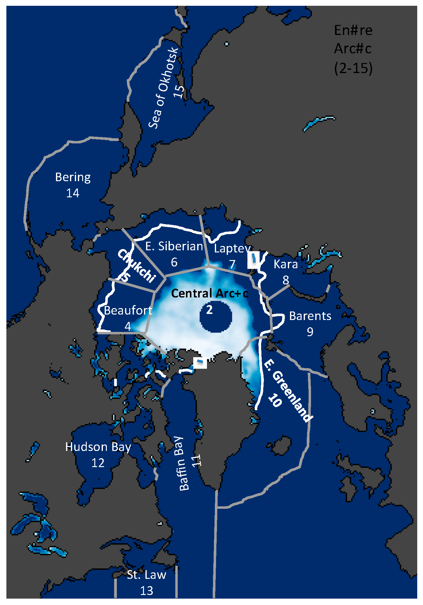
Figure 2.
Contributions to SH and LH flux variability illustrates the sensitivity of SH and LH fluxes to changes in Ts–Ta, qs–qa, and 10-m wind speed. (a,b) The perturbation analysis uses AIRS and ERA-Interim reanalysis data and their respective standardized anomalies ranging from 0 to 3σ. The standard deviations, σ, are computed for the Arctic Ocean domain average between 2003 and 2015. The sensitivity of SH and LH fluxes to the individual terms are quantified in the top, right panel as the line slope, m. (c) The average 2003–2015 September SH flux is shown in addition to the spatial distribution of the variance contributions to the September SH flux from individual changes in (d) Ts–Ta and (e) 10-m winds. Ts–Ta (10-m winds) variance contributions are determined relative to SH fluxes computed assuming climatological Ts–Ta (10-m winds) and fully varying 10-m winds (Ts–Ta).

Figure 3.
Time series for three buoys showing comparisons between in situ and AIRS-derived 2-m air temperatures. AIRS is shown in red, buoys in black and their difference (buoy-AIRS) in green.
Figure 3.
Time series for three buoys showing comparisons between in situ and AIRS-derived 2-m air temperatures. AIRS is shown in red, buoys in black and their difference (buoy-AIRS) in green.

Figure 4.
Histograms of monthly average, satellite-retrieved (a,c) LH and (b,d) SH fluxes [57] stratified by monthly average sea ice concentration from passive microwave retrievals between 2003–2015. Histograms on the bottom show the same data as the top panel with a different scale and sea ice concentrations ranging from 20–100%. The regions include 2–15 (excluding 12 and 13) in Figure 1.
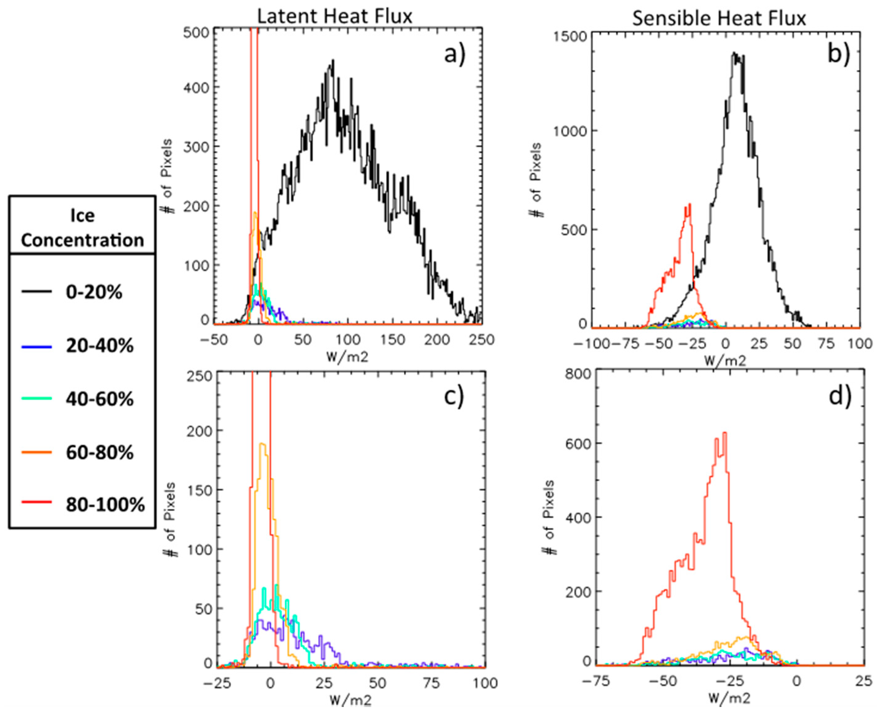
Figure 5.
Schematic summary of key interactions between turbulent fluxes and the atmosphere.
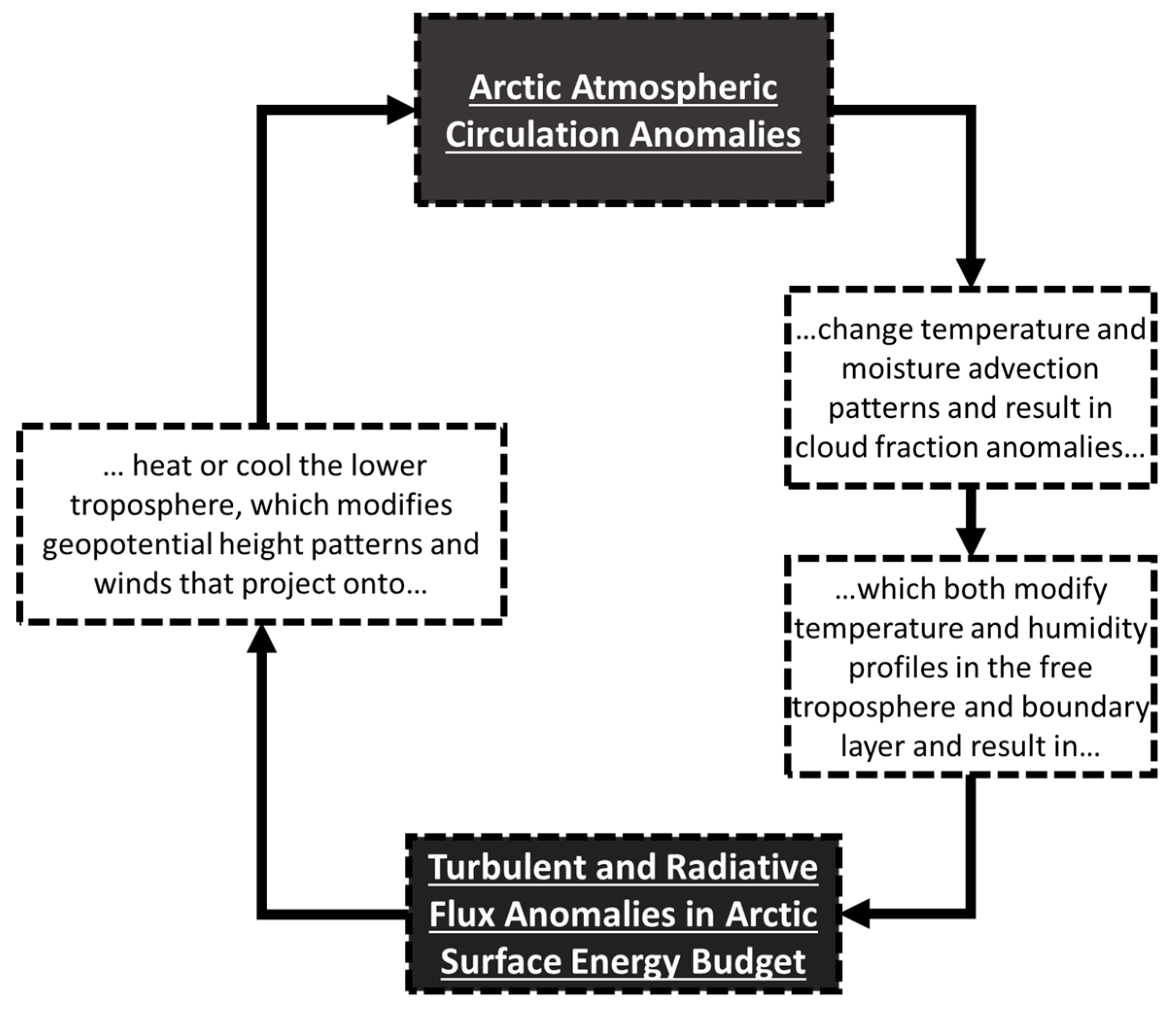
Figure 6.
Top panels show satellite-retrieved annual cycles of (a) SH and (b) LH fluxes averaged from 2003–2015 for the Arctic Ocean domain (orange line) and several interesting regions (see legend). The annual cycle of SH and LH fluxes measured during SHEBA are shown in purple. Bottom panels show the present-day annual cycle of (c) SH and (d) LH fluxes averaged over all non-land gridboxes poleward of 60° N from a 16-member CMIP5 climate model ensemble using the RCP8.5 forcing, a high-emission scenario in which greenhouse gas emissions continue to rise throughout the 21st century. The value in the (c) and (d) represent the annual, ensemble averaged SH and LH fluxes. Present-day is defined as the first 20 years of the simulation (2006–2026).

Figure 7.
Top panels show the satellite-retrieved annually-averaged SH (a) and LH (b) between 2003 and 2015 for the Arctic Ocean. Bottom panels show the present-day annually-averaged SH (c) and LH (d) fluxes poleward of 60° N from a 16-member CMIP5 climate model ensemble using the RCP8.5 forcing. Present-day is defined as the first 20 years of the simulation (2006–2026).

Figure 8.
Spatial variations of the inter-model spread represented as the inter-model standard deviation (σ) in the present-day annually-averaged (a) SH, (b) LH, and (c) Ts–Ta poleward of 60° N across a 16-member CMIP5 climate model ensemble using the RCP8.5 forcing. Present-day is defined as the first 20 years of the simulation (2006–2026).

Figure 9.
Left and center panels show the satellite-retrieved annual, Arctic domain-averaged (a) SH and (b) LH time series (orange line) between 2003 and 2015 and several other regions (see legend). (c) The probability distribution function of daily LH flux values across the Arctic Ocean for 2008 (black) and 2012 (red), the inset highlights the long positive tail.

Figure 10.
Panel (a) shows the SH flux time series for three reanalysis data sets (see legend) between 1979 and 2013 averaged over the entire Arctic (land and ocean) poleward of 60° N. Panel (c) as in (a) except showing LH flux. The spatial distribution of the annual-average (b) SH and (d) LH trends from 1979–2013 for NASA’s Modern Era Reanalysis (MERRA) are shown.
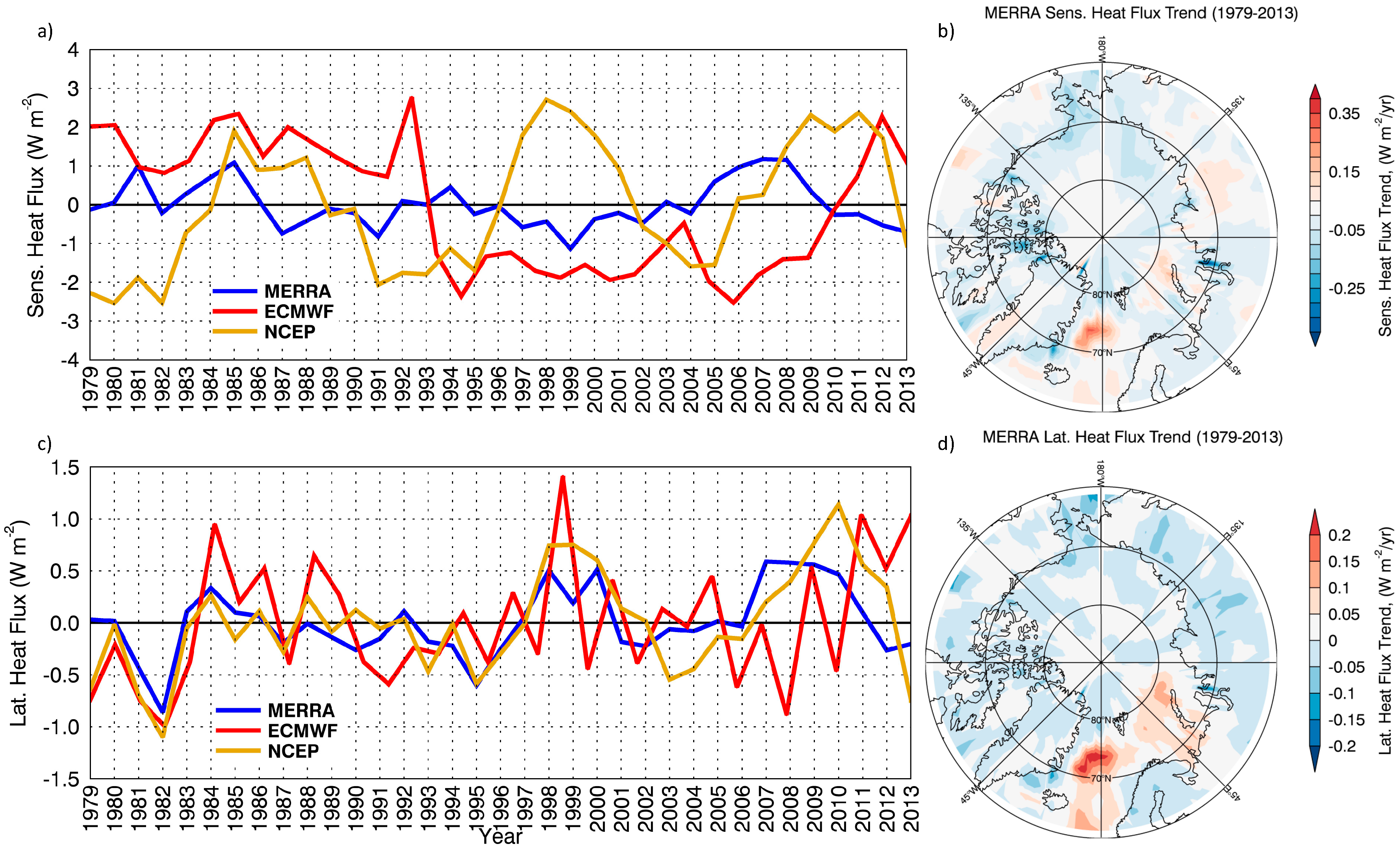
Figure 11.
Panels show the observed, seasonal trends of (a) SH and (b) LH across the Arctic between 2003 and 2015 (Units: W m−2 yr−1): March-April-May (MAM), June-July-August (JJA), September-October-November (SON), and December-January-February (DJF). Land regions are in gray and white represents trends that are not statistically significant at the 95% confidence level.
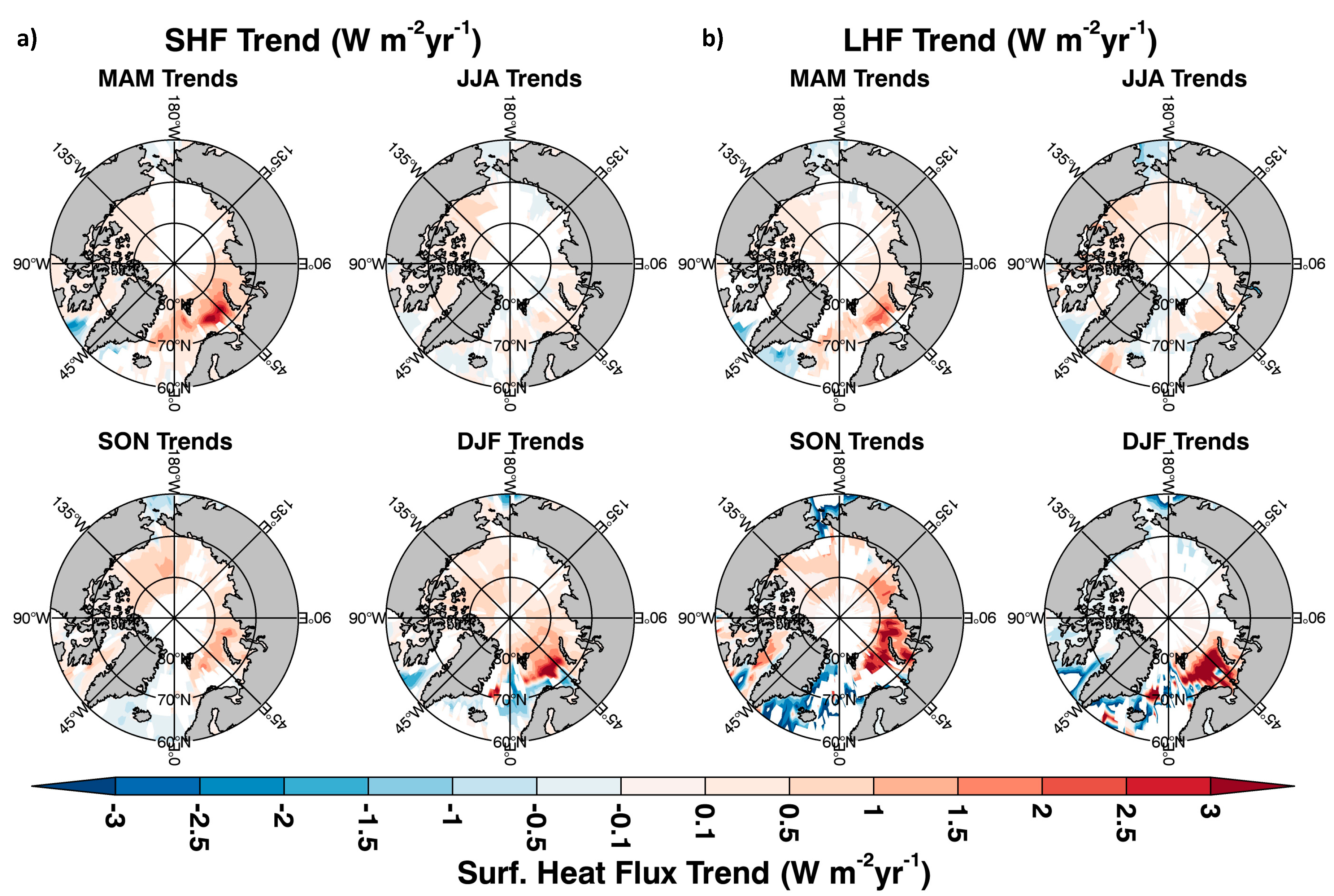
Figure 12.
Panels show the observed, seasonal trends (a) Ts–Ta, (b) qs–qa, (c) sea ice concentration, and (d) 10-m wind speed across the Arctic between 2003 and 2015. Land regions are in gray and white shows trends that are not statistically significant at the 95% confidence level using a two-sided t-test.
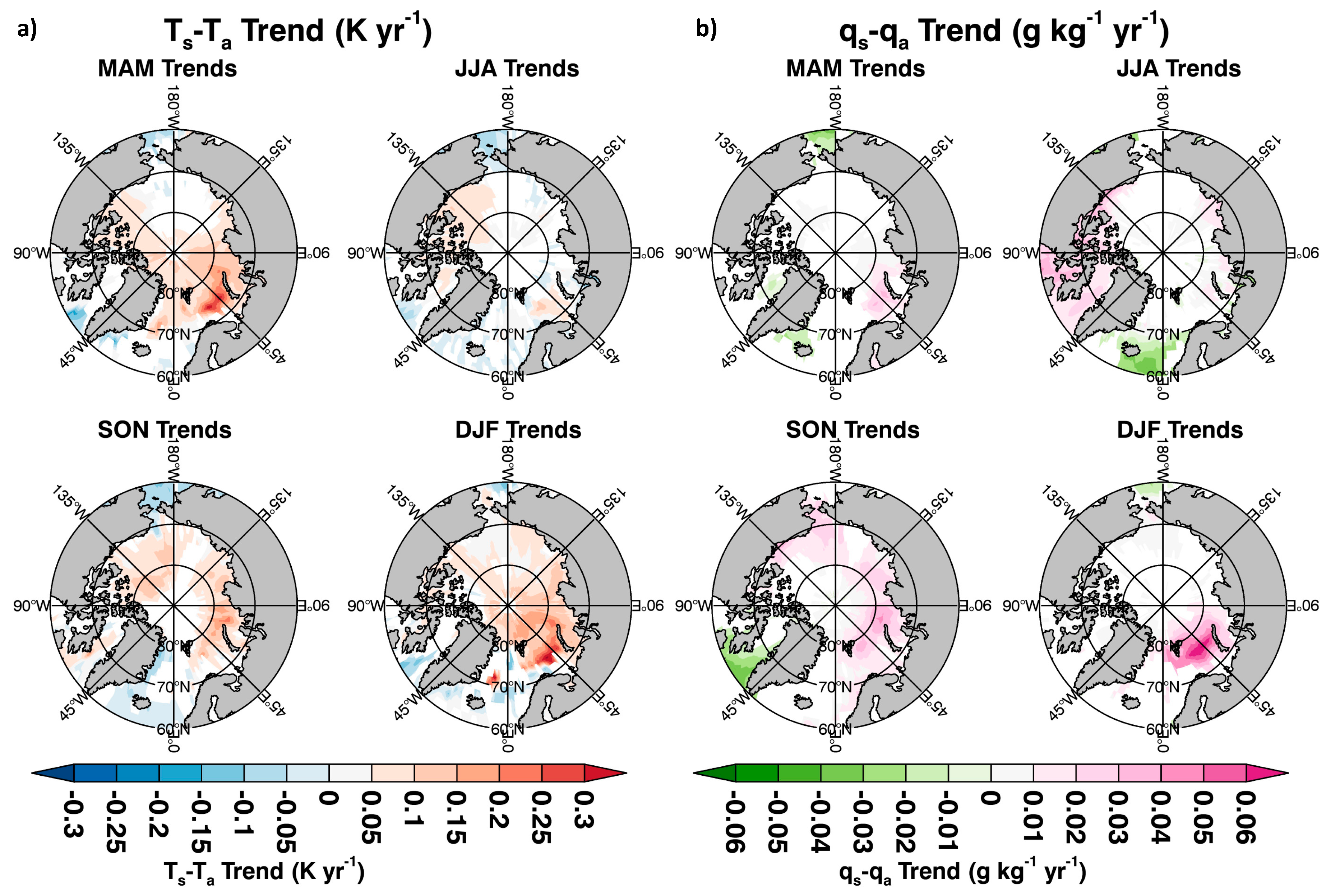

Figure 13.
Top panels show the projected annual cycle of future (a) SH and (b) LH fluxes averaged over all non-land gridboxes poleward of 60° N for RCP8.5 during the future period for 16 CMIP5 models. Bottom panels show the (c) SH and (d) LH flux differences between the future and present-day periods. Present-day is defined as the first 20 years of the simulation (2006–2026) and future is defined as the 20-year period between 2080 and 2100.
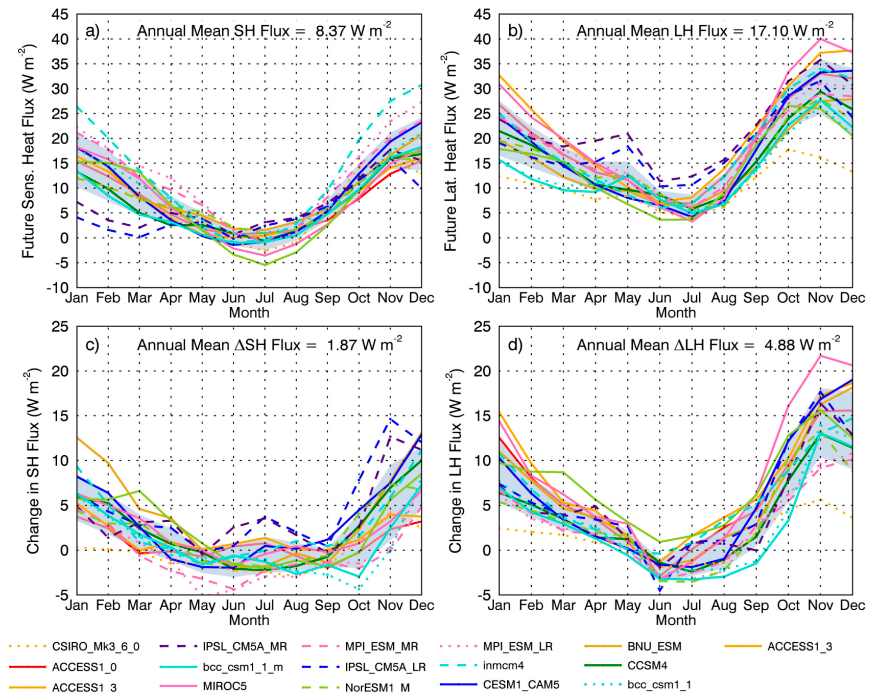
Figure 14.
Spatial variability of (a) SH, (b) LH, (c) Ts–Ta, and (d) sea ice concentration (SIC) changes between future and present-day for a 16-member CMIP5 climate model ensemble using the RCP8.5 forcing. Present-day is defined as the first 20 years of the simulation (2006–2026) and future is defined as the 20-year period between 2080 and 2100.


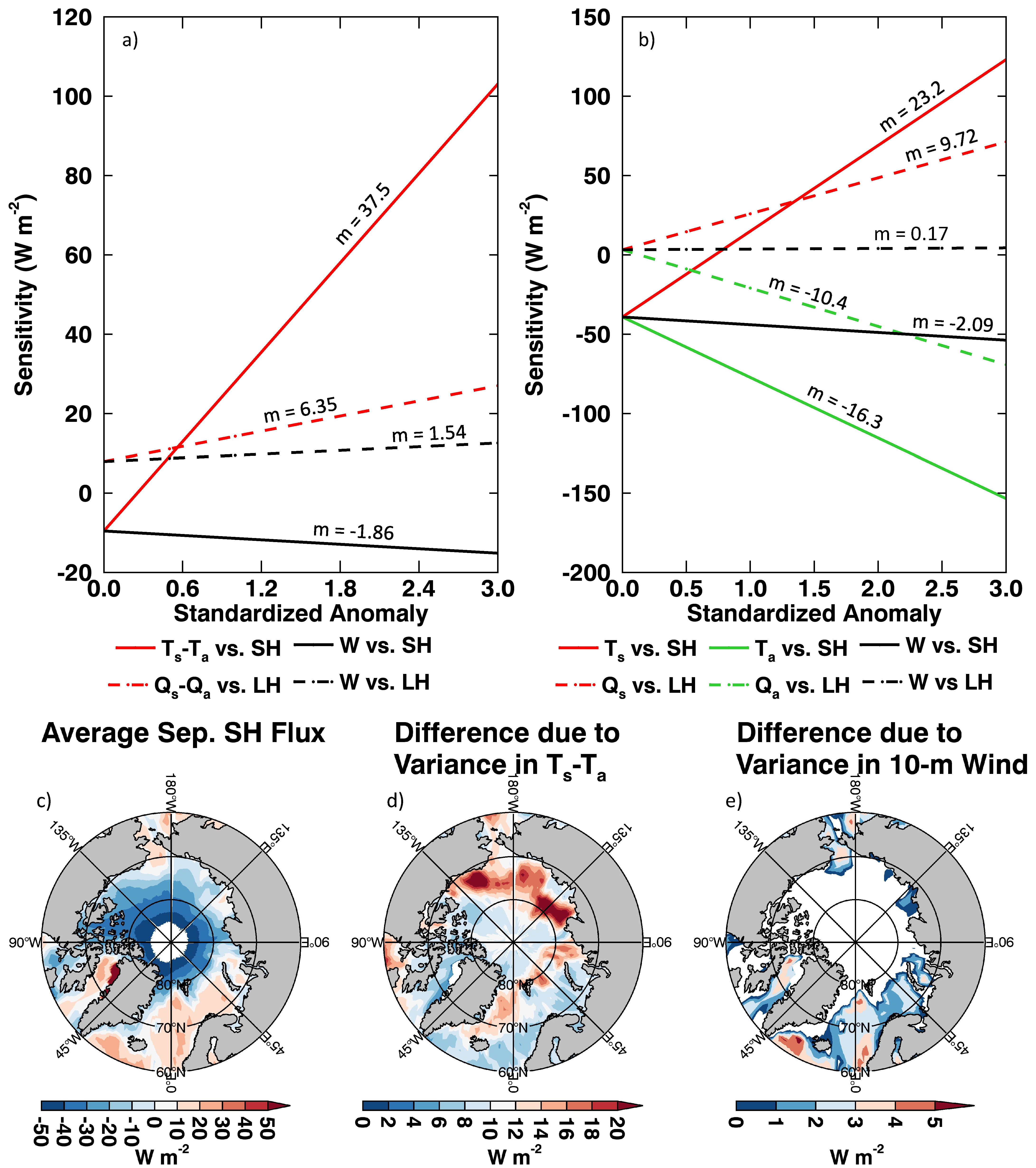
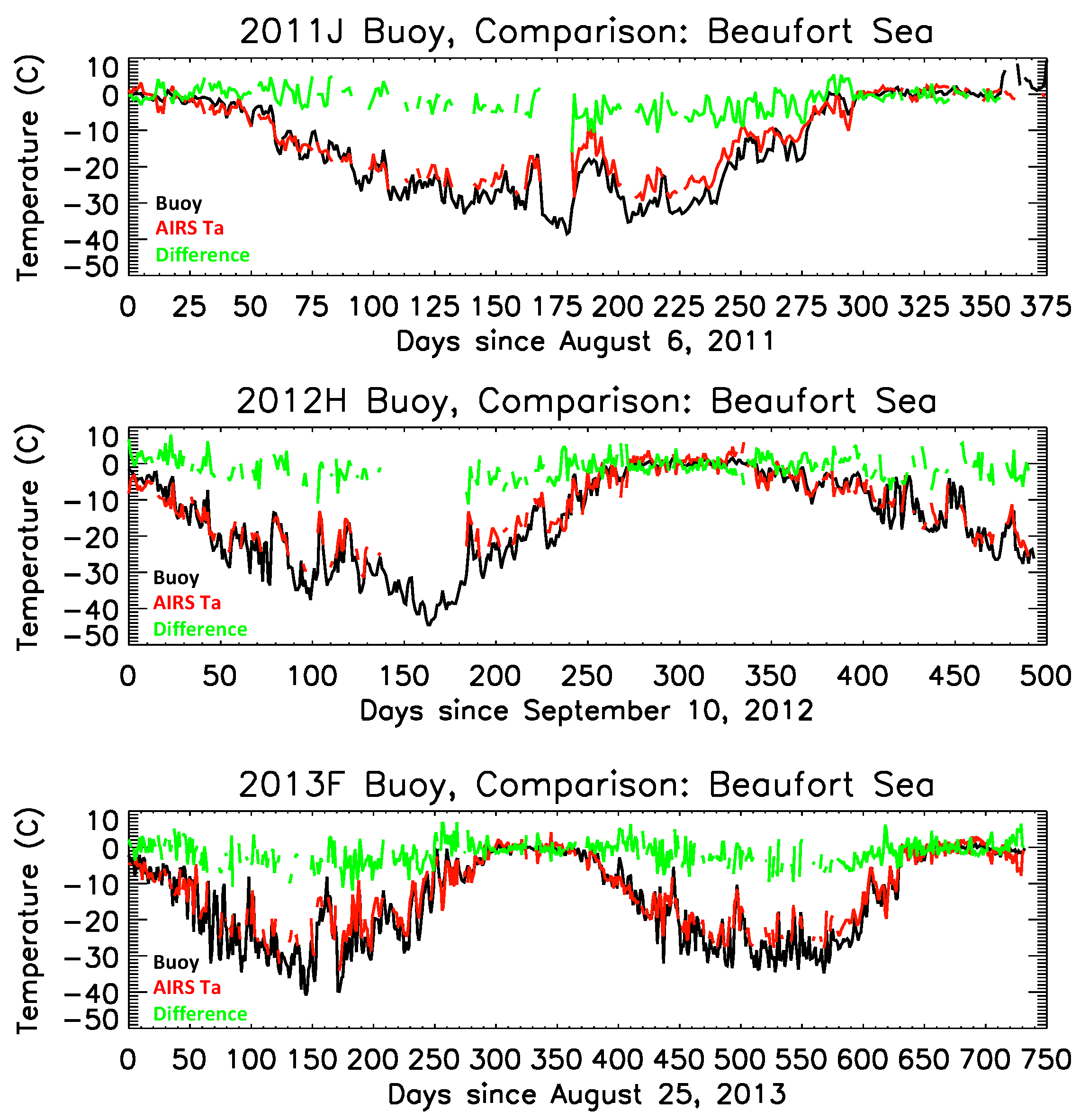
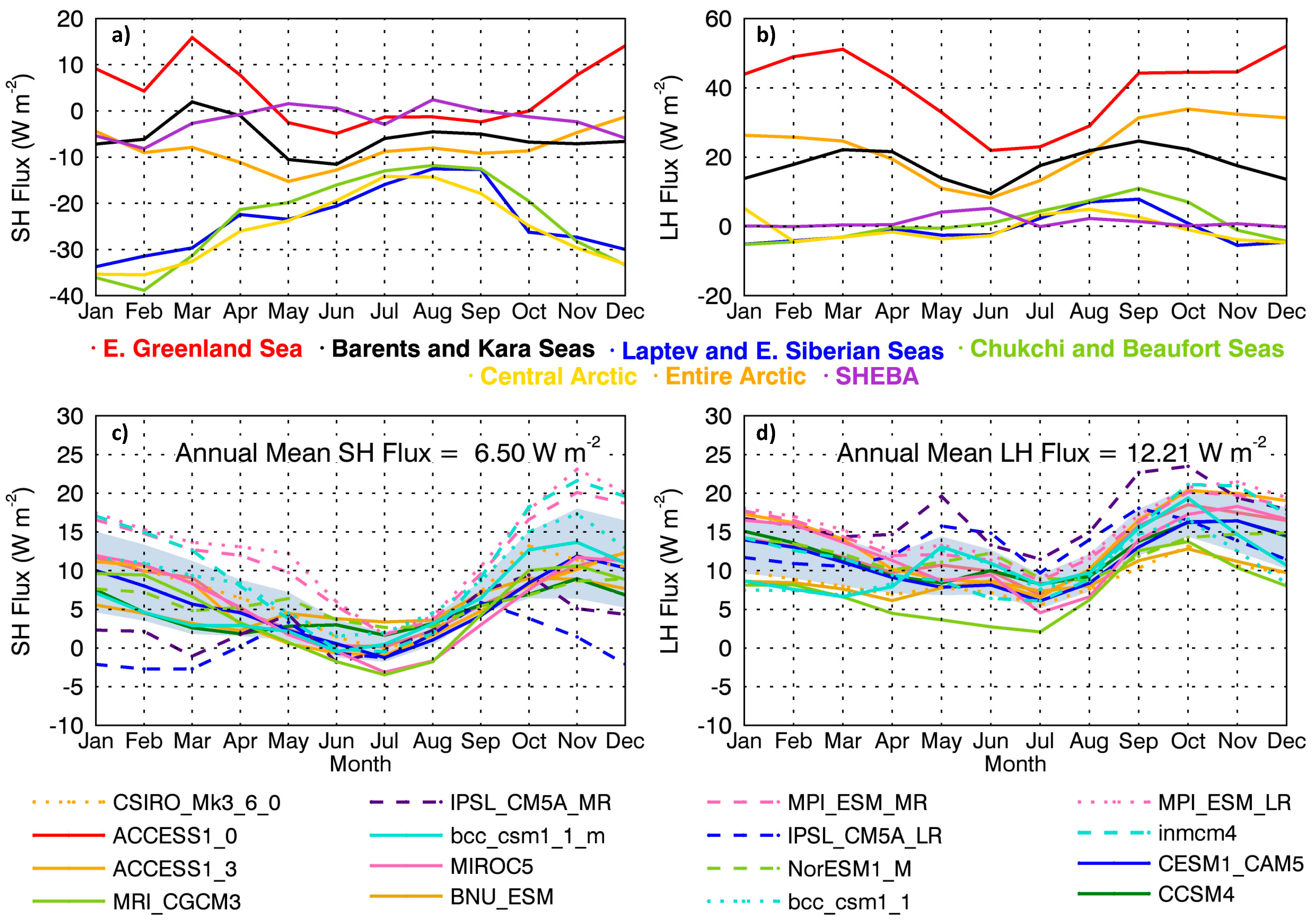
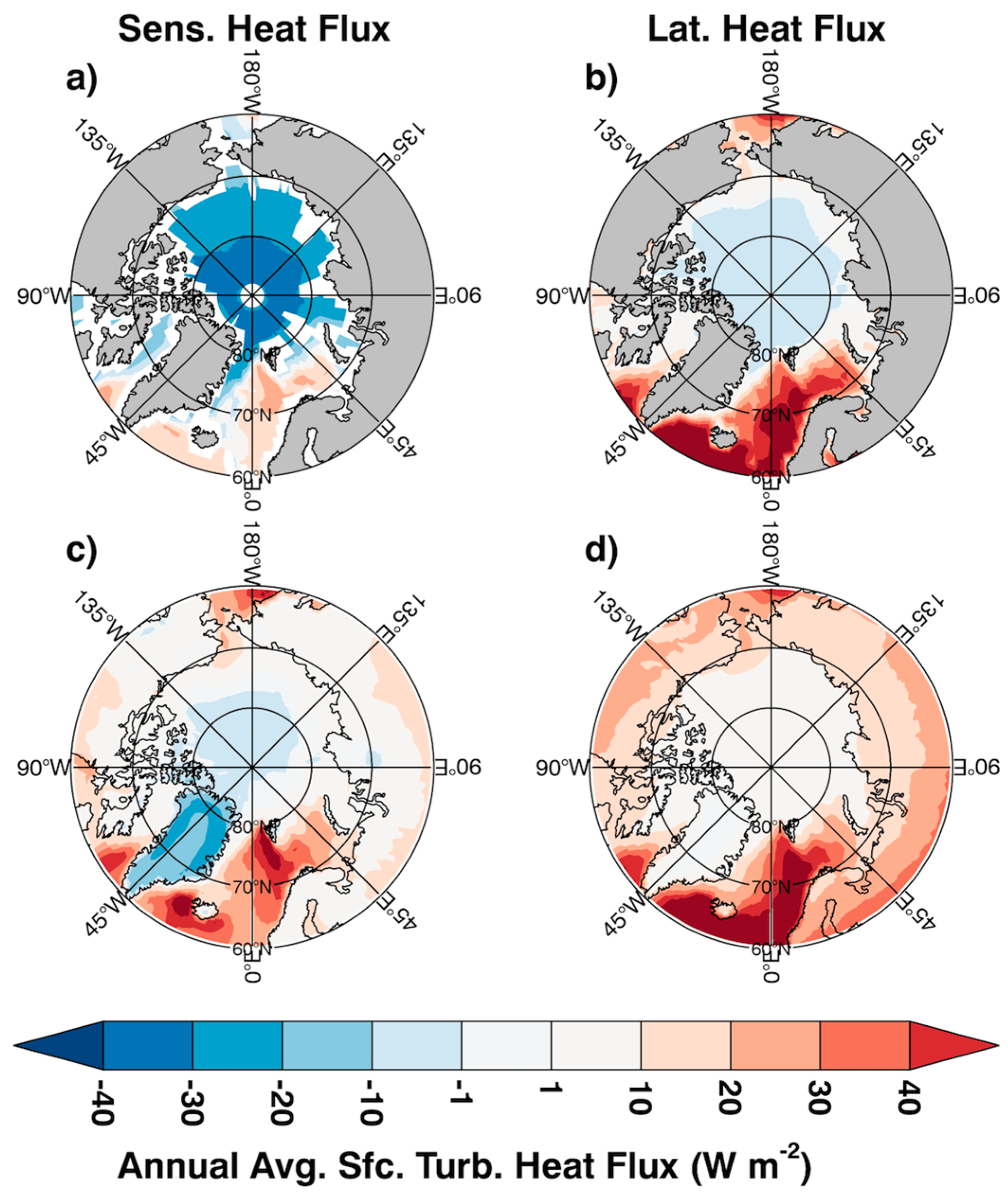
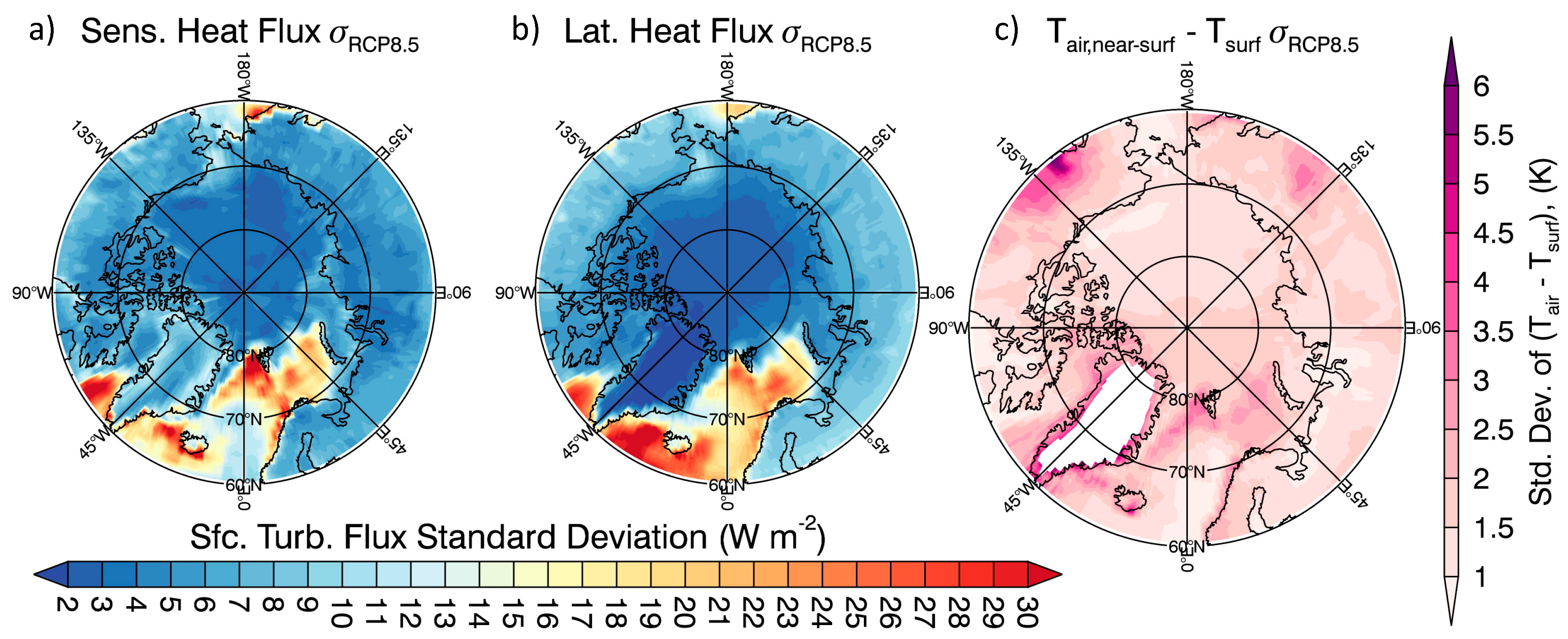
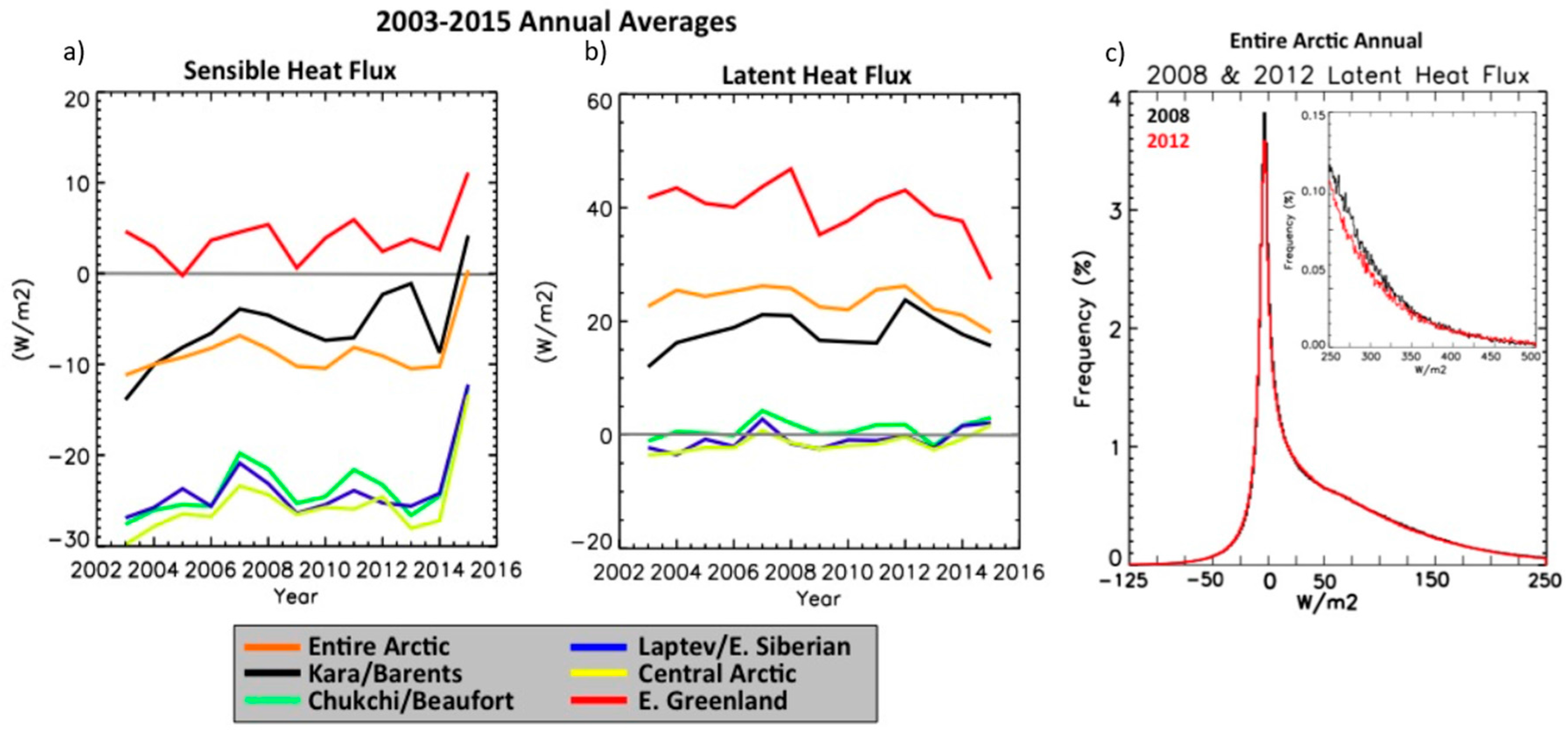
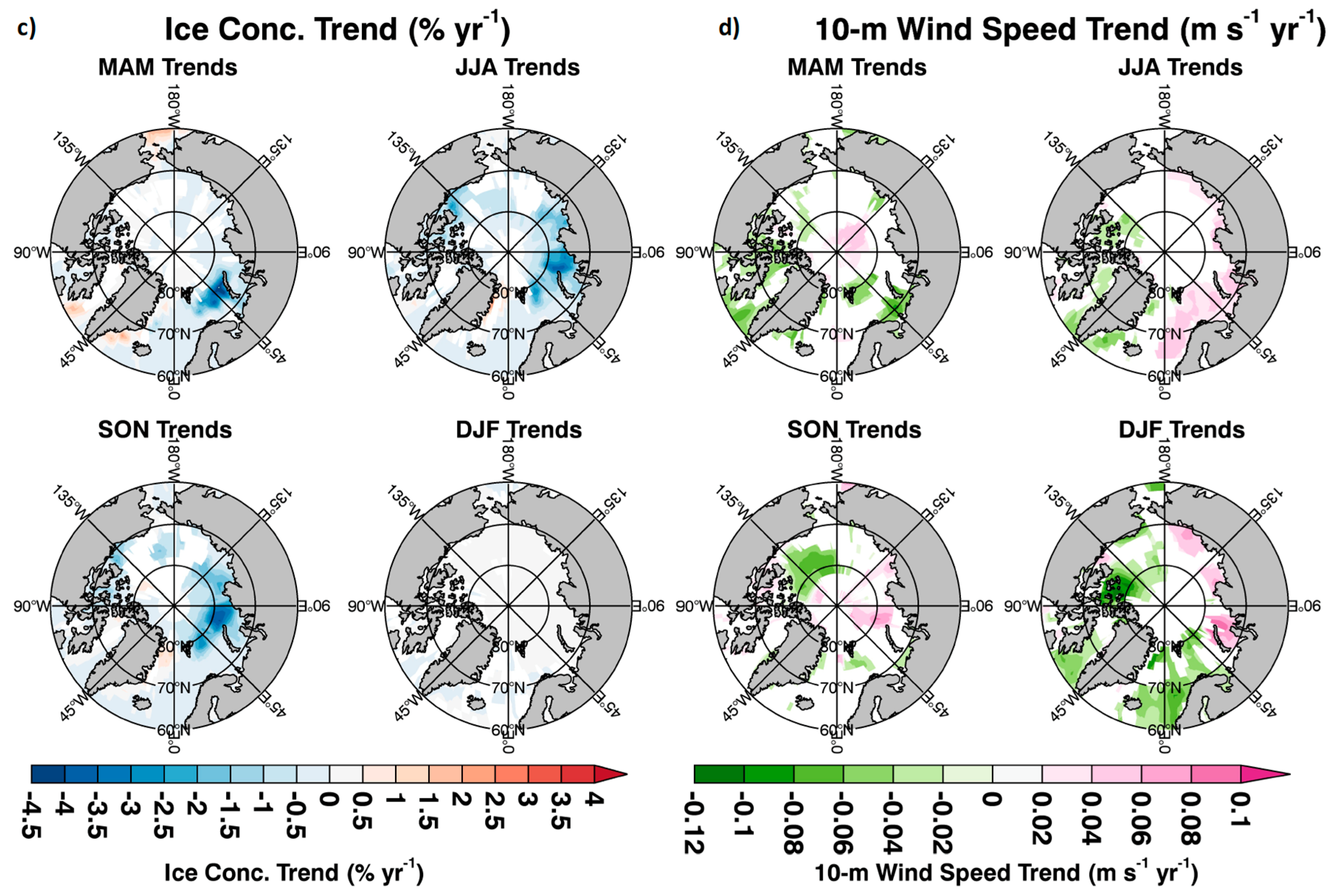
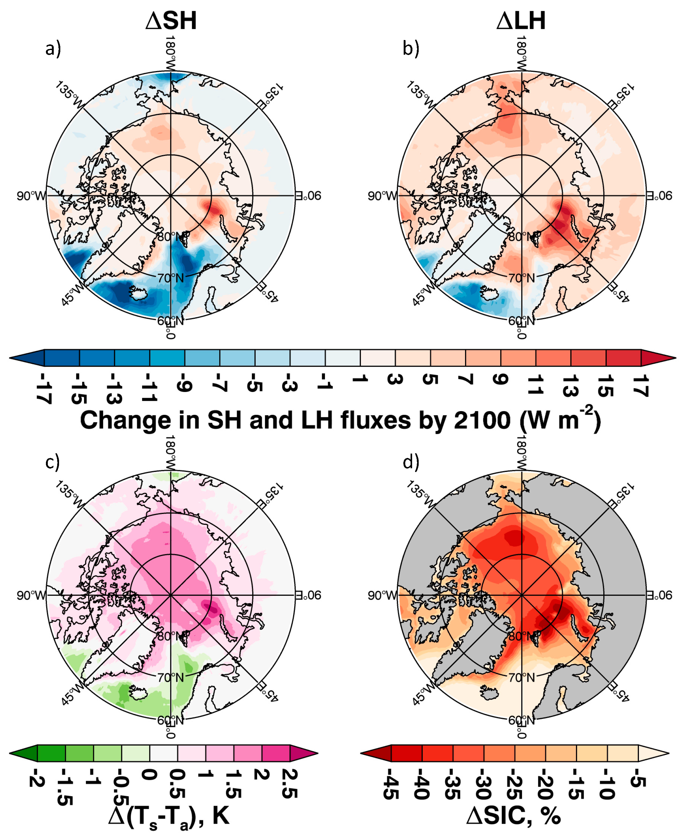
Table 1.
List of major Arctic field campaigns measuring surface radiative and turbulent fluxes over sea ice.
Table 1.
List of major Arctic field campaigns measuring surface radiative and turbulent fluxes over sea ice.
| Campaign | Duration and Location | Contribution to Understanding of Arctic Surface Processes |
|---|---|---|
| Arctic Ice Dynamics Joint Experiment (AIDJEX) | March 1975–May 1976 (main experiment). Beaufort Sea. | Early field campaign that provided in situ measurements required to calculate surface sensible heat flux in the spring and summer [95] over thick sea ice conditions. |
| Lead Experiment (LeadEx) [114] | March and April 1992. Beaufort Sea. | First coordinated field campaign measuring meteorological, surface energy budget, oceanographic, and ice measurements over multi-year sea ice and in the presence of leads in spring [114]. Measured increased sensible heat flux and increased depth of the turbulent surface layer due to the presence of leads both at the location of the lead and downwind [98]. |
| Arctic Ocean Expedition 1996 (AOE-1996) [107] | 12 July–21 September 1996. Barents and Kara Seas and central Arctic Ocean. | Provided measurements of the late-summer Central Arctic boundary layer structure and surface energy budget components, and their sensitivity to clouds and cyclonic activity in the atmosphere [9,107,115,116]. |
| Surface Heat Budget of the Arctic Ocean (SHEBA) [72,87] | October 1997–October 1998. Beaufort Sea | Only campaign to observe a full seasonal cycle. Data collected has increased understanding of seasonal cycle of surface turbulent and radiative fluxes [10] and cloud forcing [100]. Data also increased understanding of the role of the interaction of these fluxes in sea ice growth, melt, and the transitions between these states [101,102,103,117] along with assisting in developing flux-profile relationships to improve bulk surface turbulent flux calculations [88]. |
| Arctic Ocean Expedition 2001 (AOE-2001) [108] | 5 July–21 August 2001. Moored in ice floe from 2–21 August in central Arctic Ocean (main atmospheric campaign). | Expanded meteorological subprogram relative to AOE-1996. Data collected highlighted the interaction between mesoscale and synoptic-scale atmospheric variability and boundary-layer turbulence, boundary-layer structure, and surface fluxes during summer [108,118]. Data used to show frequent decoupling of low-level cloud layer from the surface and to quantify the diurnal cycle in cloud layer and near-surface parameters [118,119]. |
| Arctic Summer Cloud Ocean Study (ASCOS) [109] | 3 August–7 September 2008 Arctic Ocean north of Svalbard. | Data collected were used to examine the structures of mixed-phase low-level stratocumulus clouds coupled and uncoupled with the surface and their relationship to surface turbulent and radiative fluxes [110,111]. Data were also used to examine the co-variability of surface fluxes and sea ice freeze-up progression [58]. |
| Arctic Clouds in Summer Experiment (ACSE) [111,120] | 5 July–5 October 2014. Marginal seas north of Scandinavia and Russia, along the marginal ice zone. | Situated in the marginal ice zone in late summer and early fall, data collected showed differences in important cloud properties between the late summer and early fall. The data were also used to highlight differences in boundary layer structure over different surface types and times during the late summer and fall [111]. |
| Norwegian Young Sea-Ice Campaign (N-ICE2015) [112] | January–June 2015 Arctic Ocean north of Svalbard | Surface energy budget measurements over young, thin ice were taken during the transition from freezing to melting ice conditions, highlighting the complex relationship between clouds, winds, heat/moisture advection, and the surface ocean on surface energy components over this ice type [113,121,122]. Confirmed existence of bimodal longwave surface radiative flux distribution in January and February that also existed in SHEBA [103,123]. |
| SeaState [105] | 2 October–5 November 2015. Chukchi and Beaufort Seas. | Data collected over a sea ice formation region in autumn showed the coupling of the sea state and sea ice advance, connected through fluxes at the air-ocean-ice interface. The data also showed the importance of strong heat loss to atmosphere through surface turbulent and radiative fluxes in the sea ice formation process, especially in off-ice wind events, and the potential importance of ocean waves to sea ice formation and growth [105,106]. |
Table 2.
Summary of RMS errors in temperature and specific humidity with respect to available in situ and satellite reference data.
Table 2.
Summary of RMS errors in temperature and specific humidity with respect to available in situ and satellite reference data.
| Reference Data | RMS Error | ||
|---|---|---|---|
| AIRS V6 | ERA-Interim | ||
| Skin temperature (K): Sea Ice | Tara | 2.3 | 4.9 |
| IceBridge | 3.3 | 8.9 | |
| Skin temperature (K): Open Water | AVHRR (All) | 1.2 | 1.7 |
| 2-m Air temperature (K): Sea Ice * | 12 Ice Mass Buoys (all) | 3.41 | |
| 2009A (North Pole) | 1.00 | ||
| 2009F (Central Arctic) | 4.65 | ||
| 2010A (North Pole) | 3.69 | ||
| 2010F (Beaufort Sea) | 3.88 | ||
| 2011I (Beafort Sea) | 2.41 | ||
| 2011J (Beaufort Sea) | 3.70 | ||
| 2012H (Beaufort Sea) | 4.13 | ||
| 2013B (Central Arctic) | 3.40 | ||
| 2013F (Beaufort Sea) | 3.46 | ||
| 2013H (Central Arctic) | 3.63 | ||
| 2014I (Beaufort Sea) | 3.29 | ||
| 2015G (Central Arctic) | 3.63 | ||
| Specific Humidity (g kg−1): Sea ice | Tara | 0.55 | 0.45 |
| Specific Humidity (g kg−1): Sea ice | RV Polarstern | 0.52 | 0.31 |
| Latent Heat Flux (W m−2) | N-ICE2015 | 0.74 | |
| Sensible Heat Flux (W m−2) | N-ICE2015 | 5.32 | |
* 2-m air temepratures are derived from 1000 hPa AIRS air temperatures and determined via the iterative method described above.
Table 3.
Summary of SH and LH Trends (Units: W m−2 yr−1) and 2003–2015 average values in parentheses (Units: W m−2). Each region is numbered corresponding to Figure 1.
Table 3.
Summary of SH and LH Trends (Units: W m−2 yr−1) and 2003–2015 average values in parentheses (Units: W m−2). Each region is numbered corresponding to Figure 1.
| Region | MAM | JJA | SON | DJF | Annual | |
|---|---|---|---|---|---|---|
| Entire Arctic (2–15 w/o 12 & 13) | SH | 0.39 (−17.1) | 0.063 (−10.1) | 0.15 (−8.6) | 0.37 (−21.6) | 0.22 (−16.2) |
| LH | −0.12 (19.2) | 0.002 (11.1) | 0.013 (30.8) | −0.07 (25.4) | −0.014 (17.1) | |
| Sea of Okhotsk (15) | SH | −0.17 (−3.5) | 0.15 (−8.5) | −0.15 (16.1) | 0.45 (24.7) | −0.002 (−7.0) |
| LH | −0.50 (32.0) | −0.17 (31.1) | 0.05 (79.1) | 0.56 (45.1) | −0.005 (45.9) | |
| Bering Sea (14) | SH | 0.00 (−2.8) | −0.24 (−5.1) | −0.80 (20.7) | −1.10 (20.9) | −0.47 (9.8) |
| LH | −0.93 (41.5) | −0.61 (25.7) | −1.27 (82.8) | −0.90 (67.8) | −0.74 (50.7) | |
| Baffin Bay (11) | SH | −0.35 (−6.0) | 0.008 (−9.2) | 0.53 (−12.8) | 0.13 (2.40) | 0.07 (−5.1) |
| LH | −0.83 (42.4) | −0.36 (17.5) | 0.93 (34.8) | −0.85 (55.5) | −0.16 (31.3) | |
| E. Greenland Sea (10) | SH | 0.63 (2.0) | −0.09 (−1.1) | −0.35 (4.48) | −0.03 (7.31) | 0.12 (−3.6) |
| LH | −0.16 (53.0) | −0.10 (16.5) | −0.70 (45.8) | −0.61 (58.3) | −0.30 (38.6) | |
| Barents Sea (9) | SH | 1.40 (−16.8) | 0.17 (−8.0) | 0.86 (−16.6) | 1.13 (−13.8) | 0.77 (−11.7) |
| LH | 0.98 (11.1) | 0.31 (11.0) | 0.61 (11.1) | 0.90 (10.6) | 0.66 (10.93) | |
| Kara Sea (8) | SH | 0.79 (−34.7) | 0.03 (−9.3) | 0.77 (−28.2) | 0.56 (−37.9) | 0.39 (−28.4) |
| LH | 0.31 (−2.6) | 0.18 (11.2) | 0.75 (−2.26) | 0.36 (−6.61) | 0.34 (−0.49) | |
| Laptev Sea (7) | SH | 0.49 (−31.6) | 0.12 (−14.5) | 0.44 (−27.1) | 0.33 (−37.1) | 0.27 (−28.3) |
| LH | 0.20 (−4.6) | 0.35 (0.94) | 0.47 (−4.11) | 0.08 (−5.0) | 0.23 (−3.14) | |
| E. Siberian Sea (6) | SH | 0.18 (−25.3) | −0.20 (−13.5) | 0.56 (−28.4) | 0.28 (−37.1) | 0.30 (−31.7) |
| LH | −0.08 (−0.35) | 0.22 (−2.6) | 0.31 (−1.91) | −0.002 (−5.0) | 0.12 (−2.75) | |
| Chukchi Sea (5) | SH | −0.09 (−17.4) | 0.10 (−13.5) | 0.53 (−26.7) | 0.40 (−42.0) | 0.30 (−28.5) |
| LH | −0.16 (3.2) | 0.07 (3.8) | 0.008 (10.3) | −0.03 (−4.21) | −0.01 (2.87) | |
| Beaufort Sea (4) | SH | 0.34 (−29.7) | 0.50 (−22.7) | 0.57 (−32.4) | 0.46 (−43.4) | 0.52 (−30.8) |
| LH | 0.20 (−5.6) | 0.52 (−4.5) | 0.28 (−4.86) | 0.05 (−6.0) | 0.24 (−4.84) | |
| Can. Arch. (3) | SH | 0.33 (−26.1) | 0.30 (−10.4) | 0.18 (−23.2) | 0.51 (−33.7) | 0.28 (−22.6) |
| LH | 0.22 (−5.8) | 0.53 (8.9) | 0.24 (−2.88) | 0.01 (−4.09) | 0.20 (−0.81) | |
| Central Arctic (2) | SH | 0.46 (−40.2) | 0.17 (−21.0) | 0.57 (−36.0) | 0.65 (−49.5) | 0.37 (−37.0) |
| LH | 0.16 (−8.2) | 0.20 (−9.3) | 0.23 (−10.9) | 0.15 (−7.63) | 0.15 (−8.80) |
Table 4.
Present-day (2006–2026) and projected changes (2080–2100 minus present-day, signified by Δ) in surface temperature (Ts), near-surface air temperature (Ta), SH, LH, and sea ice concentration (SIC) averaged across all non-land gridboxes in the Arctic domain (60°–90° N) for 16 CMIP5 climate models using the RCP8.5 forcing.
| Model | Ts | ΔTs | Ta | ΔTa | SH | ΔSH | LH | ΔLH | SIC | ΔSIC |
|---|---|---|---|---|---|---|---|---|---|---|
| ACCESS1-0 | 262.23 | 8.94 | 263.45 | 7.82 | 6.44 | 0.73 | 12.88 | 6.22 | 42.4 | −21.8 |
| ACCESS1-3 | 262.95 | 9.10 | 264.08 | 7.94 | 5.77 | 1.65 | 13.98 | 7.64 | 41.80 | −24.50 |
| BNU-ESM | 261.19 | 9.52 | 263.34 | 8.87 | 5.28 | 4.00 | 8.97 | 6.11 | 43.3 | −22.6 |
| CCSM4 | 261.52 | 7.10 | 264.06 | 5.40 | 4.62 | 2.23 | 12.18 | 3.88 | 46.40 | −17.20 |
| CESM1-CAM5 | 260.23 | 8.59 | 262.89 | 6.96 | 5.47 | 3.25 | 11.50 | 5.83 | 46.6 | −22 |
| CSIRO-Mk3-6-0 | 257.31 | 6.22 | 259.88 | 5.07 | 7.25 | −0.36 | 8.81 | 1.55 | 51.40 | −7.00 |
| IPSL-CM5A-LR | 261.58 | 7.69 | 263.49 | 6.33 | 0.41 | 4.73 | 13.27 | 5.48 | 45.4 | −19.5 |
| IPSL-CM5A-MR | 264.27 | 6.47 | 265.71 | 5.35 | 2.97 | 3.83 | 17.03 | 4.87 | 39.70 | −17.70 |
| MIROC5 | 261.42 | 9.38 | 261.87 | 8.72 | 5.52 | 2.02 | 12.74 | 8.09 | 46.6 | −25.7 |
| MPI-ESM-MR | 263.54 | 6.53 | 264.76 | 6.49 | 11.79 | −0.45 | 14.90 | 2.92 | 42.80 | −19.00 |
| MPI-ESM-LR | 263.52 | 6.45 | 264.50 | 6.39 | 12.92 | −0.30 | 15.67 | 2.90 | 43.1 | −18.5 |
| MRI-CGCM3 | 258.44 | 7.88 | 261.44 | 5.96 | 4.71 | 2.44 | 7.23 | 7.35 | 51.30 | −18.4 |
| NorESM1-M | 260.77 | 7.47 | 262.66 | 6.77 | 5.85 | 1.94 | 12.23 | 3.46 | 47 | −17.4 |
| BCC-CSM1-1-M | 262.48 | 5.76 | 263.37 | 5.12 | 5.55 | 0.94 | 11.07 | 2.66 | 44.00 | −14 |
| BCC-CSM1-1 | 261.74 | 6.45 | 262.03 | 5.95 | 8.91 | 0.56 | 10.22 | 3.45 | 46.6 | −16.2 |
| INMCM4 | 264.13 | 5.75 | 266.29 | 4.99 | 10.52 | 2.74 | 12.74 | 5.74 | 42.90 | −18.2 |
| Ensemble Avg | 261.71 | 7.45 | 263.37 | 6.51 | 6.50 | 1.87 | 12.21 | 4.88 | 45.10 | −18.70 |
| Std Dev | 1.91 | 1.30 | 1.61 | 1.27 | 3.20 | 2.27 | 3.15 | 2.00 | 3.23 | 4.40 |
© 2018 by the authors. Licensee MDPI, Basel, Switzerland. This article is an open access article distributed under the terms and conditions of the Creative Commons Attribution (CC BY) license (http://creativecommons.org/licenses/by/4.0/).
Share and Cite
MDPI and ACS Style
Taylor, P.C.; Hegyi, B.M.; Boeke, R.C.; Boisvert, L.N. On the Increasing Importance of Air-Sea Exchanges in a Thawing Arctic: A Review. Atmosphere 2018, 9, 41. https://doi.org/10.3390/atmos9020041
AMA Style
Taylor PC, Hegyi BM, Boeke RC, Boisvert LN. On the Increasing Importance of Air-Sea Exchanges in a Thawing Arctic: A Review. Atmosphere. 2018; 9(2):41. https://doi.org/10.3390/atmos9020041
Chicago/Turabian StyleTaylor, Patrick C., Bradley M. Hegyi, Robyn C. Boeke, and Linette N. Boisvert. 2018. "On the Increasing Importance of Air-Sea Exchanges in a Thawing Arctic: A Review" Atmosphere 9, no. 2: 41. https://doi.org/10.3390/atmos9020041
Note that from the first issue of 2016, this journal uses article numbers instead of page numbers. See further details here.