1. Introduction
The well-known urban heat island (UHI) phenomenon is used to describe cities that are generally hotter than their rural surroundings. The main candidate causes considered to be responsible for this phenomenon include the presence of dense urban surfaces that absorb more solar radiation, the release of anthropogenic heat from the combustion of fuels, and the trapping of longwave radiation due to taller buildings and smaller street widths inside the urban canopy [
1,
2,
3]. Excessive heat release exacerbates urban environmental pollution and human discomfort [
4,
5]. With gradually rising air temperatures in cities possibly caused by drastic reductions in greenery areas, land use planning has become critical in determining the environmental quality [
6,
7].
As a local heat source over urban surfaces, an UHI can drive corresponding thermal circulation patterns. UHI-induced circulation can be investigated through not only observational and numerical studies but also theoretical analysis, in which the UHI is considered a thermal response of the low-level atmosphere to a specified surface or is represented by near-surface heating. There are two common theoretical practices in dealing with UHI circulation. The first practice is to simplify the problem into a two-dimensional system to solve the analytic solutions. For example, Olfe and Lee [
8] carried out steady, linearized flow calculations to estimate the vertical temperature profiles over a heated area representing a city. Kimura [
9] investigated the effects of uniform flows on two-dimensional heat island convection by obtaining the steady solutions of the linearized vorticity and thermodynamic equations and then discussed the calculations for non-viscous and neutral fluids. Lin and Smith [
10] analytically solved for the time-dependent, linearized response of a stratified, moving fluid to an elevated, local heat source turned on as a pulse. They found that the solution exhibits a region of positive displacement moving downstream as the steady state is approached while a negative displacement develops near the stationary heat source. Baik [
11] applied a linear analytic model to study the response of a stable, stratified atmosphere to specified low-level heating in a constant shear flow. The results suggested the existence of typical gravity waves produced in response to a local heat source in the presence of environmental flow.
The second practice is to analytically solve the three-dimensional equations by applying a Fourier transform, which reduces the system into a partial differential equation for the vertical velocity in the wavenumber space. For example, Lin [
12] obtained a second-order partial differential equation to investigate the airflow over an isolated heat source with applications to the dynamics of V-shaped clouds. By introducing the Rayleigh friction coefficient, Sang et al. [
13] obtained a fourth-order equation and discussed the influences of various atmospheric conditions, such as basic flows and eddy diffusivity. Han and Baik [
14] derived a second-order equation with a solution that reveals a typical internal gravity wave field that includes low-level upward motion downwind of the heating center.
Three-dimensional theoretical studies are beneficial for better understanding UHI circulation. However, to solve such problems analytically, the turbulent friction is neglected or is set to a Rayleigh friction form. Considering that UHI circulation is mainly thermally induced, Li et al. [
15] and Li and Chao [
16] specified a declining temperature profile and derived the analytic solution of the three-dimensional circulation without using a Fourier transform. Their results suggested an exact physical relationship between the thermal distribution and its induced circulation. However, the declining temperature profile is too rough in certain cases. For example, a stable temperature inversion layer, which could exacerbate the air pollution [
17], often occurs at low elevation [
18] in heavy haze days. Especially, observation in Santiago of Chile [
19] emphasized the importance of a surface inversion, which could occur 263 days per year. Therefore, it is necessary to investigate how the UHI circulation distributes in the temperature inversion case and how it differs from the UHI circulation in the non-temperature inversion (NTI) case. This study aims to extend the finding of previous studies [
15,
16] to a more general case to identify the influence of the inversion layer and to compare the corresponding discrepancies with the NTI case.
2. Analytic Solution
UHI circulation is a thermally induced phenomenon and is significant under weak synoptic systems [
20]. Both observational and theoretical studies suggest that it decreases with increasing wind speeds [
13,
21]. Therefore, it is appropriate to discuss UHI circulation in a stationary atmospheric background, which can directly remove the impacts of basic flows but explicitly retain the thermal forcing of a UHI.
The Boussinesq equations under a stationary atmosphere background are as follows:
where
are the air temperature, pressure, and velocity vector deviations with respect to the stationary atmospheric background,
is the air density of the stationary atmospheric background,
is the Coriolis parameter,
is the gravitational constant of acceleration,
is the thermal expansion coefficient of the air, and
is the vertical diffusion coefficient.
Following [
15,
16], we set
and substitute Equation (3) into Equations (1) and (2) to eliminate the pressure
. Then, Equations (1) and (2) can be written as
The upper boundary, where the atmosphere is stationary and non-viscous, is taken at infinity. Therefore, when
, we can obtain
Then, the integral of Equation (5) can be written as
Rewriting Equation (7) in an operator form
where the operator
,
,
, and
is the Ekman elevation. The boundary conditions are taken as
where
is the boundary condition operator. Applying the Green’s function method, the analytic solution of Equation (8) is
where
is the Green’s function with the following specific form
To obtain the analytic solution of Equation (10), the specific form of
should be solved. Our previous works [
15,
16] assumed an NTI profile, which portrays a temperature profile that exponentially declines with increasing altitude. According to this assumption, they obtained an elegant analytic solution of Equation (10). Although the influence of surface heating eventually disappears with increasing height, the detailed distribution might be complex. For example, as mentioned in the first section, a typical inversion layer at a low level could be observed on many hazy days [
18] and even on certain normal days [
22]. However, an NTI profile is not enough to depict the temperature inversion layer. To overcome this shortcoming, we introduce a surface temperature inversion (STI) profile containing an inversion layer ranging from the urban surface to a certain height, namely
where
is the reference UHI intensity,
is the non-dimensional horizontal distribution, and
is the non-dimensional vertical distribution.
and
are parameters that control the size of the urban area. For convenience, we set
to represent a circular urban area.
and
are three introduced parameters, where
is a non-negative integer.
and
control the height and intensity of the inversion layer, respectively. This is a more general form of the vertical temperature distribution. By specifying different parameter values, this approach can reproduce both the NTI case and the STI case. For example, by setting
, we can easily reduce Equation (12) to the NTI case used by [
15,
16].
The specific form of
can then be obtained by integrating Equation (12) vertically
where
is the incomplete
function, where
is an integral variable. Since
is a non-negative integer, the specific integration value can be determined as
where
is the following power series
Substituting Equation (13) and the Green’s function in Equation (11) into the solution of Equation (10) reveals the following
The notations
and
are introduced in this study to shorten the expression in Equation (16) and are written as
where
denotes the
kth-order derivative of
, and
denotes
itself. Separating Equation (16) into its real and imaginary parts, we obtain
where
The vertical velocity can be solved by setting
where
represents the horizontal Laplace operator. At this point, we can finally explicitly express the UHI circulation as a function of the temperature distribution. The expressions are similar in form to the derivation presented by [
15,
16]. The solutions suggest that the induced circulation can be determined once the surface heating distribution is given.
Particularly, when
, the specific forms of
and
reduce to
In addition, when
, the specific forms of
and
are
where
It is easily seen that both and have similar forms. In contrast, with increasing values of , more terms will appear. Therefore, we do not list the specific forms for . Interested readers can easily write them out.
Comparing with the previous studies [
15,
16], the only but most important difference lies in the vertical temperature distribution governed by Equation (12) which extends the simple declining temperature profile to a more general form. Such a difference does not invalidate the physical settings and mathematic derivations. Therefore, it naturally inherits the validation from the previous studies [
15,
16]. The theoretical model also had been testified against a numerical model [
16], the results of which could be analogical to testify the current research for both the sea breeze and the urban heat island circulation are local thermal forced motion.
3. Results and Discussion
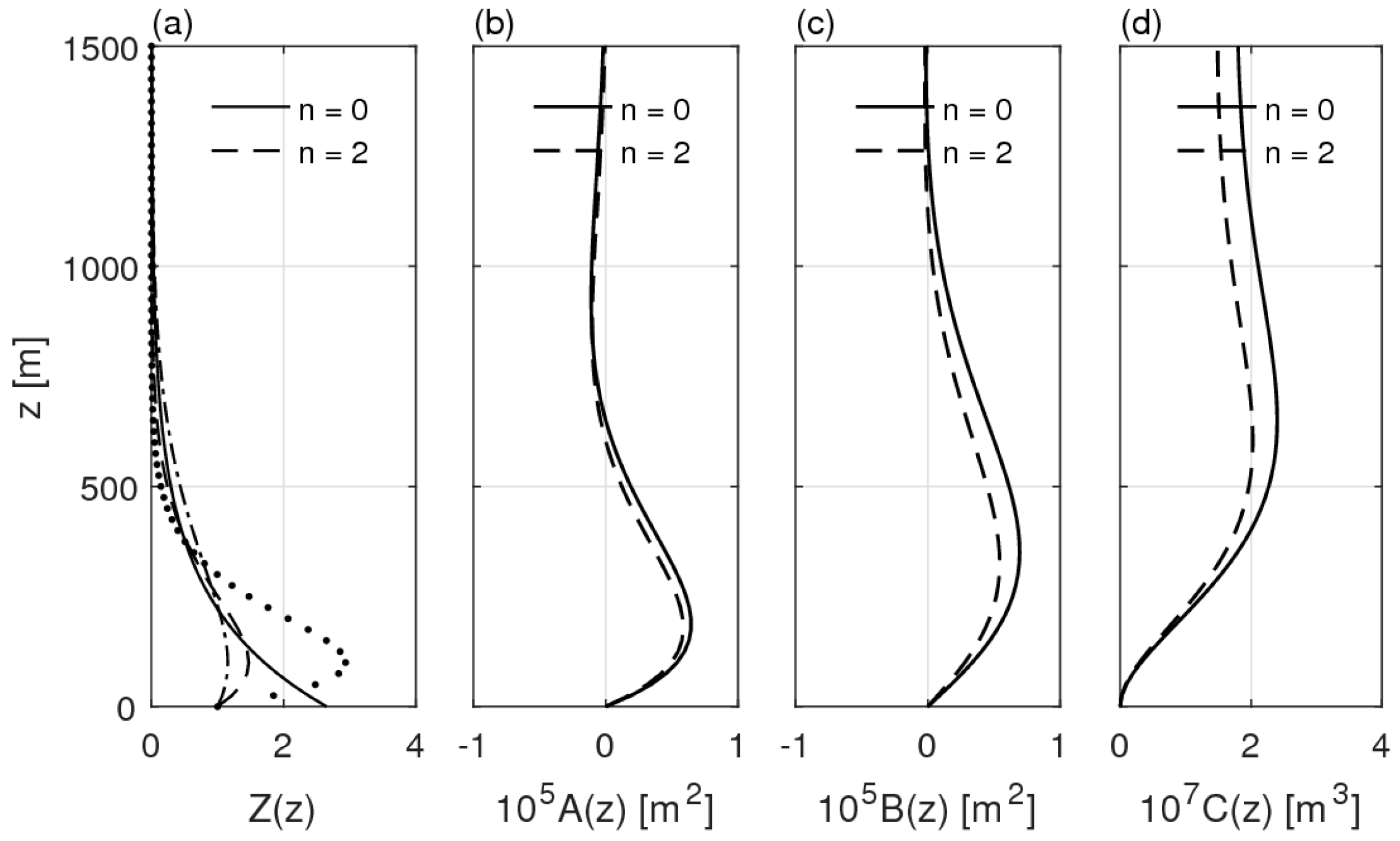
The above mathematical derivation extends UHI circulation from an NTI case to an STI case. Then, how is UHI circulation distributed in an STI case, and how does it differ from the circulation in an NTI case? In this section, we establish a known STI profile with a 100-m-thick inversion layer above the urban surface (
Figure 1a, dashed line) to calculate the corresponding UHI circulation. To identify the influences of the inversion layer, we further appoint a known NTI profile (
Figure 1a, solid line). The main discrepancy between the two profiles occurs in the inversion layer and their difference is negligible above the inversion lid. According to the two temperature profiles, the UHI intensity is weaker in STI case than in NTI case.
Once the temperature distributions are given, the vertical distribution of the UHI circulation can be determined.
Figure 1b–d portrays the vertical distributions of
,
, and
.
and
control the heights where the u-wind and v-wind approach their maximum values, while
determines the height of the maximum vertical velocity value. For example,
reaches its maximum value at a height of approximately 250 m (
Figure 1b). Similarly, the maximum values of
(
Figure 1c) and
(
Figure 1d) occur at heights of approximately 300 m and 600 m, respectively. As is observed from the figure, there are no obvious differences between the STI case (
Figure 1b–d, dashed lines) and the NTI case (
Figure 1b–d, solid lines). Meanwhile, there does exist one particular difference between the two cases. The maximum values of
,
, and
and their heights in the NTI case are larger and higher, respectively, than those in the STI case. This demonstrates that an STI could weaken the speed values or the UHI circulation intensity, even though such weakening is not very significant.
Three parameters are introduced to construct the STI. These parameters regulate the intensity and the height of the inversion layer and influence the maximum horizontal and vertical velocity values and their heights as discussed above. When
are fixed, both the intensity and the height of the inversion layer increase with increasing
; when
is fixed, both the intensity and the height of the inversion layer decrease with increasing
; and when
are fixed, both the intensity and the height of the inversion layer increase with increasing
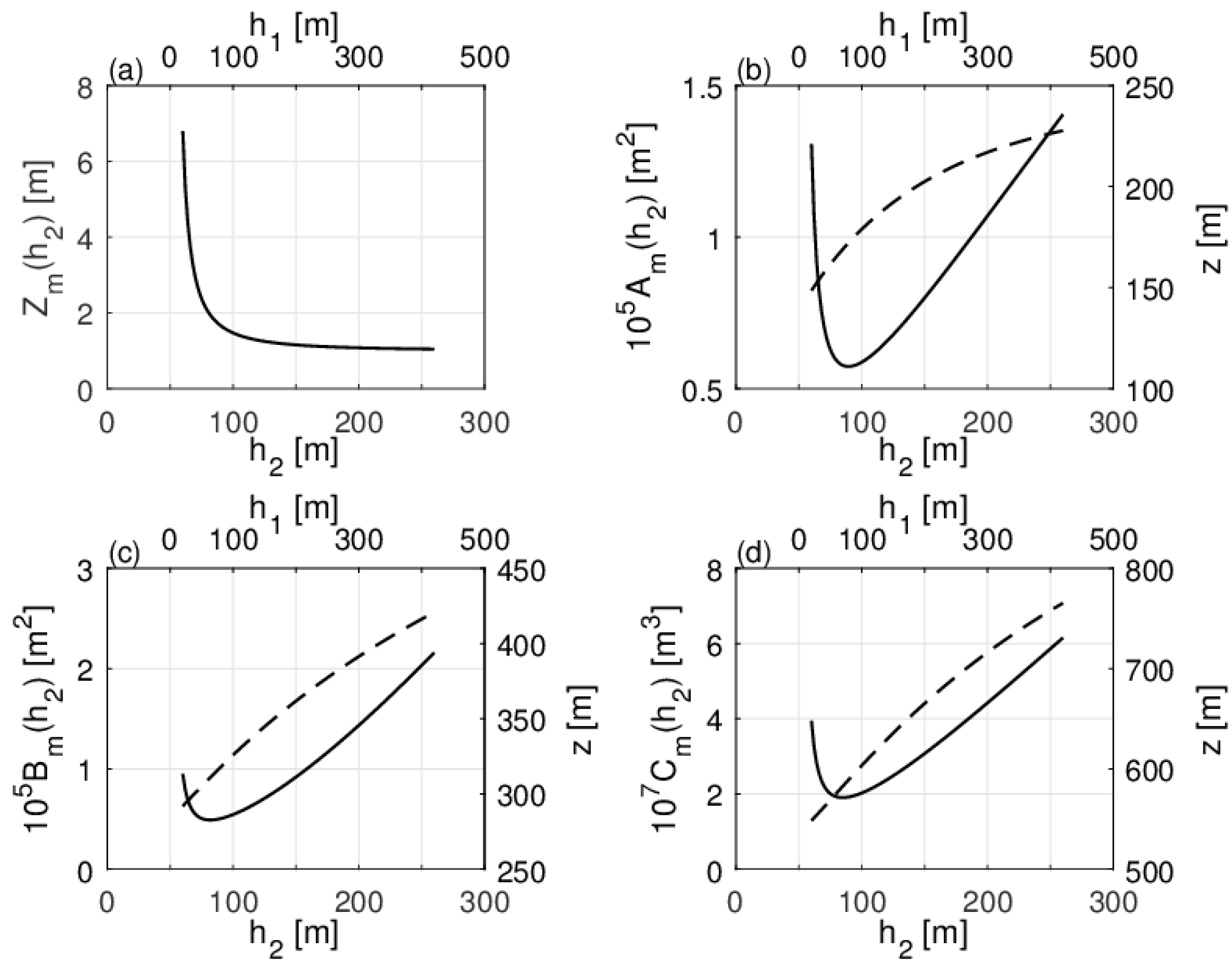
. It would be complex to individually discuss the influence of each parameter. Therefore, we analyze the sensitivities of the parameters by fixing the height of the inversion layer. For example, we set
. This means that the thickness of the inversion layer is 100 m and that
are linearly correlated. According to
, both
and
have inversely proportional roles in controlling the inversion intensity. In
Figure 1a, when
is fixed at 2, the dotted, dashed, and dash-dotted lines represent values of
varying from 70 m, to 100 m, and to 150 m, respectively. Meanwhile, the inversion intensity weakens from 2.9, to 1.5, and to 1.2. Therefore, a larger
(or
) value corresponds to a weaker inversion intensity and a smaller lapse rate above the inversion lid or a larger vertical influence of the temperature above the inversion lid. Specifically, the inversion intensity is approximately 6 when
is equal to 60 m, and the intensity decreases to 1 when
increases to 200 m (
Figure 2a). The maximum value of
(shortened as
) occurs at increasingly higher levels (
Figure 2b, dashed line) with increasing values of
. In contrast,
decreases to a minimum value when
increases to 90 m and then increases with a continuously increasing
(
Figure 2b, solid line), thereby showing a typical V-shaped variation pattern. This V-shaped variation pattern of
could be interpreted as the combined effect of a weakening inversion intensity and a strengthening temperature influence above the inversion lid. When the inversion intensity is decreasing from a larger value to a smaller value, the decreasing temperatures outweigh the increased contribution from the decreasing lapse rate above the inversion lid. This combined effect makes
decrease. However, as the inversion intensity continues to weaken, a limited weakening of the inversion intensity is not enough to offset the increased contribution from an increasingly smaller lapse rate above the inversion lid. Therefore,
stops decreasing and begins to increase. The maximum value of
(shortened as
) (
Figure 2c) and the maximum vertical velocity value of
(
) (
Figure 2d) show similar V-shaped variation patterns. To summarize, the shape and intensity of the STI profile could influence not only the maximum values of each velocity component but also the height at which the velocity components approach their maximum values.
According to Equation (18), the maximum value of the u-wind is determined both by A and by B. If the position of a point in an urban area is fixed, the maximum u-wind is then determined by a combination of A and B. In certain special cases, the maximum u-wind value relies only upon either A or B. For example, if a point is located along the x-axis, the differential of against y is equal to zero. Therefore, the maximum u-wind value is determined only by A. Similarly, if a point is located along the y-axis, the maximum u-wind value is then determined by B. Because both and decrease and then increase with a weakening inversion intensity, we could imply that the maximum value of the u-wind would decrease and then increase with a weakening inversion intensity.
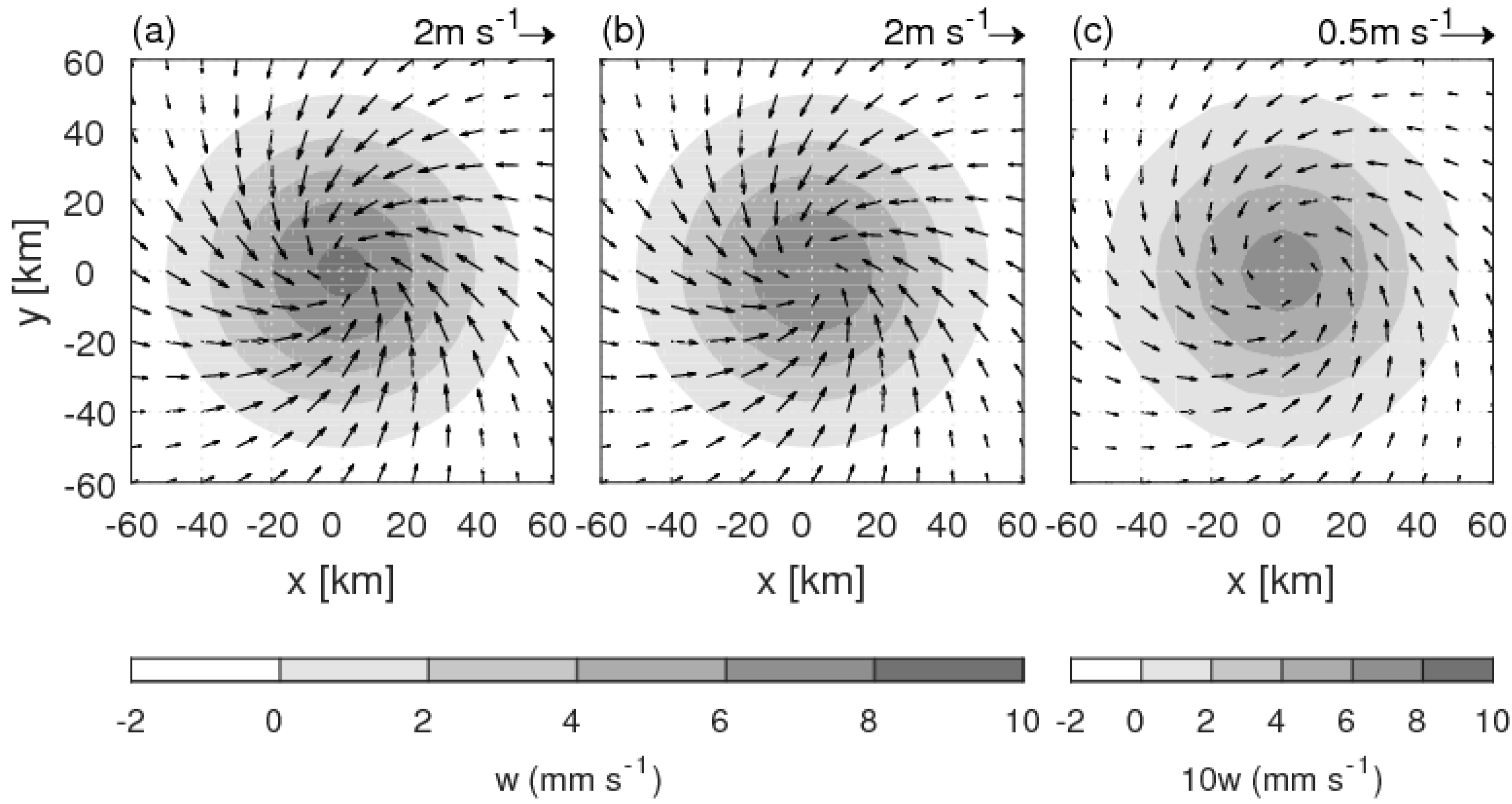
The horizontal distribution of the UHI circulation depends on the horizontal derivatives of the temperature (
). Therefore, there is no distribution difference between the two cases when specifying the same horizontal temperature distribution.
Figure 3a–c portrays the corresponding horizontal distributions of the UHI circulation for both cases and their differences at a height of 100m. As shown in the figure, the horizontal winds and vertical velocity are essentially distributed equivalently, and both exhibit a typical cyclonic circulation with updrafts (shaded) related to the heating center and winds that are blowing anticlockwise (vectors). For both cases, the maximum wind speed and vertical velocity are approximately 2 m s
−1 and 8 mm s
−1, respectively. Although the horizontal distribution is the same, the UHI circulation in the NTI case (
Figure 3a) is stronger than that in the STI case (
Figure 3b). This originates from the discrepancy between the vertical distributions of the horizontal winds and vertical velocity that is analyzed in
Figure 1. The difference in the wind, which blows anticlockwise, is approximately 0.5 m s
−1, while the vertical velocity difference is approximately 1 mm s
−1 (
Figure 3c). The UHI circulation distributions for the other two STI cases presented by the dotted and dash-dotted lines in
Figure 1a are also calculated (figure omitted). The results suggest that a stronger inversion intensity benefits to a stronger circulation cell, which could be confirmed by observational and numerical experiments (e.g., see [
23,
24]).
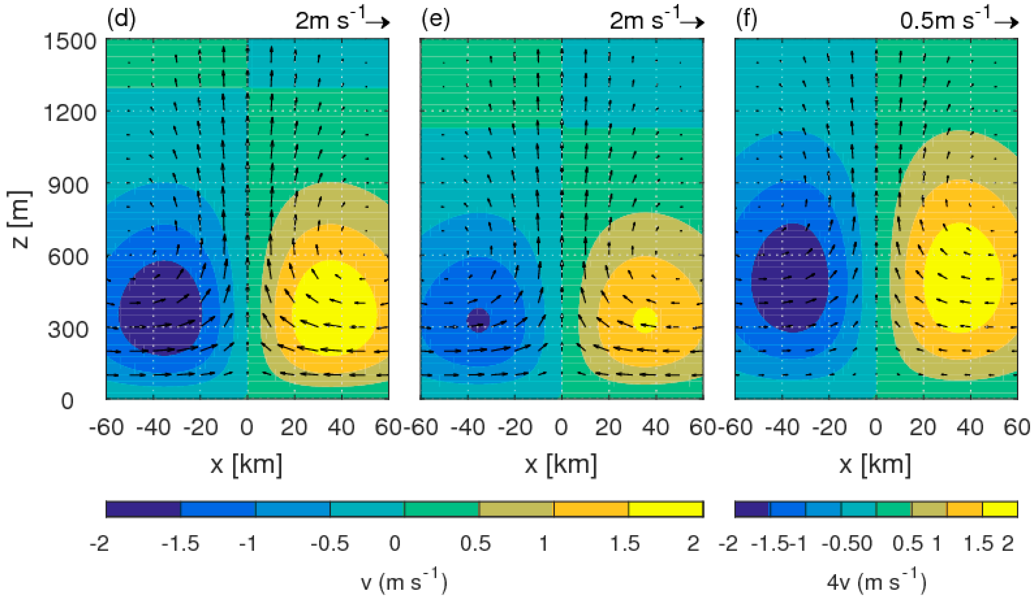
The vertical structure of the UHI circulation also shows typical heat-driven circulation (
Figure 3d,e, vectors). The air is heated in the lower level, which is accompanied by a blowing u-wind converging towards the heating center to compensate the air mass loss there. The driven updraft and u-wind strengthen and then weaken with gradually increasing heights. Upon reaching a certain height, the u-wind reverses its direction and begins to diverge from the heating center to its surroundings, where the outgoing air sinks to the ground. Finally, a converging u-wind forms at the lower level to closethe circulation cell, which is a typical vertical UHI circulation cell centered at a height of approximately 700 m. A southerly wind blows in the region where x > 0, while a northerly wind prevails in the region where x < 0 (
Figure 3d,e, shaded). This further demonstrates that the wind forms a cyclone at the lower level while blowing anticlockwise and forms an anticyclone at the upper level while blowing clockwise. The UHI circulation in the NTI case (
Figure 3d) is stronger and higher than that in the STI case (
Figure 3e). Their difference (
Figure 3f) looks like the cases themselves, and therefore, no detailed analysis is provided.
4. Summary
This study aims to solve an analytic solution for UHI circulation in the temperature inversion profile and determine the difference in UHI circulation between the temperature inversion and NTI profiles. To fulfil these goals, we introduce an STI profile constructed from the product of exponential and power functions. The STI profile is a more general form that includes three introduced parameters controlling the intensity, height, and shape of the inversion layer. The STI profile can be reduced to the NTI profile when the parameter is set to zero. It is easy to analytically express the vertical integral of the temperature distribution as an incomplete function whose specific form could be expressed as the sum of a power series by applying integration by parts. Then, we substitute the incomplete function into motion equations to eliminate temperature-related terms, thereby simplifying the problem into a second-order differential equation containing only one variable. We elegantly express the velocity field as a function of the temperature distribution by applying the Green’s function to analytically solve the problem. The solutions are formally the same as those in our previous works.
We specify a definite STI profile with a 100-m-thick inversion layer above the urban surface to investigate how UHI circulation performs in an STI. To identify the influences of the temperature inversion layer, we also appoint a definite NTI profile, which has one tiny difference with the STI profile at a height of 100 m. The calculation results suggest that there is no significant discrepancy in the vertical distributions of the two temperature profiles. Both of the corresponding velocity components behave with similar shapes and approach similar maximum values at a similar height. However, the maximum velocity component values and their corresponding heights in the NTI case are larger and higher, respectively, than those in the STI case. This implies that given analogous STI and NTI profiles, the STI profile would help to drive a stronger and higher UHI circulation cell.
A sensitivity test demonstrates that the maximum value of each velocity component will decrease to a minimum value and then increase with increasing values of (or ), which is the parameter denoting the lapse rate above the inversion lid, when specifying the inversion layer height. As (or ) grows from a smaller value to a relative larger value, the inversion intensity weakens dramatically, which could lead to a downward trend in the velocity values or UHI circulation intensity. As (or ) continues to grow, the weakening effect it introduces to the inversion intensity is compensated by the enhanced influence of the vertical temperature distribution above the inversion lid. Therefore, UHI circulation stops weakening and begins strengthening again. The height at which each velocity component approaches its maximum value is uplifted with increased values of (or ), suggesting that UHI circulation could approach a higher level.
The horizontal and vertical distributions of the UHI circulation cell both show a typical heat-driven cyclonic circulation pattern. Wind at the lower level blows anticlockwise towards the heating center, where updrafts prevail; meanwhile, wind at the upper level blows clockwise towards the surroundings, where downdrafts exist. The closed circulation cell is centered at a height of approximately 700 m with a wind speed and vertical velocity on the order of 2 m s−1 and 8 mm s−1, respectively. There is no significant difference in the values and patterns between the two temperature distributions.


