1. Introduction
Data assimilation over the mountains is made challenging by the difficulties in modeling the land and atmosphere at all scales, and because observations in mountainous environments include details below the spatial scales resolved by operational models. For example, modeling the land and atmosphere over the mountains includes errors due to the representation of subgrid-scale and grid-scale terrain using discrete grid cells, and the absence of heterogeneity in the parameterizations of the land–atmosphere exchanges. This paper provides an overview of some of the important challenges to effective data assimilation in the mountains, focusing on near-surface data assimilation in both the atmosphere and the land. We then identify some opportunities to address these challenges with modeling studies, use of current and proposed observing networks, and future field campaigns.
Systematic and/or large
departures of a model forecast from observations (i.e.,
innovations in data assimilation parlance) reduce the potential benefits of data assimilation. Large departures violate assumptions of linear perturbations and Gaussian statistics that are the foundation of most modern data assimilation systems. Systematic departures indicate bias in the model and/or observations, which if not adequately addressed will violate the assumptions of optimal assimilation, leading to sub-optimal and likely biased output [
1,
2]. However, near-surface and land data assimilation in the mountains is characterized by systematically large departures (see e.g., [
3], for a recent look at near-surface biases in the mountains) resulting from heterogeneity, associated errors of representativeness of observations, and model inadequacy. Historically, the response has been to discard observations where large systematic departures exist, without considering whether the observation or the model is primarily responsible.
Systematically large departures reveal where the greatest model and/or observation errors are to be found. Many reasons exist for the tendency towards larger assimilation departures in mountainous areas. Mountains can exert strong forcing on the atmosphere at a range of scales, from local to planetary, and inadequacies in modeling the interactions of forcing can lead to large departures. Although intermittent effects of mountains on the atmosphere are clear through the depth of the troposphere, mountains persistently force the near-surface atmosphere. The presence of complex terrain adds significant complexity to the relationship between surface sensible and latent heat fluxes and the boundary layer structure. Mountains can also modify atmospheric momentum more directly than flat terrain, and across a much wider range of scales. Additionally, the land surface models used in atmospheric models all neglect flow of soil moisture between grid cells, and also typically neglect (or greatly simplify) surface run-off and groundwater processes [
4,
5,
6]. These neglected processes are more likely to lead to large departures in mountainous areas, where the steeper topographic gradients will more strongly drive lateral flows of water.
Effective observing systems in mountainous areas are far from simple to construct. Representativeness errors—defined in data assimilation as the errors from scales not simulated by a model but present in observations, and attributed to observation error—are also acute in the mountains. Details in terrain are absent below the model discretization scale, and representativeness error is demonstrably large when model grid spacing is at the scale of tens of kilometers. Representativeness errors are not precisely treated in current systems, and it is plausible that information contained in existing observations is still not adequately extracted in today’s data assimilation systems.
Conversely, as weather modeling capabilities begin to resolve circulations at km-scale or smaller, the density of near-surface observations has not kept pace. Much as a model grid cell can not represent all the scales within it, the observing network itself cannot adequately sample the heterogeneous flow around complex terrain. Finer model grid spacing means that more state components in a model are less connected to relatively sparse observations, or are connected in ways that simple covariance models or small ensembles do not handle well.
The complexities of land–atmosphere interactions in the mountains, combined with model inadequacy from resolution limitations and parameterizations, lead to suboptimal data assimilation in the mountains. This paper explores key challenges to optimal data assimilation in the mountains, and identifies opportunities to advance its utility there. While none of the issues discussed here are necessarily unique to mountainous environments, they are made more extreme by the exaggerated heterogeneity in the mountains. Hence, the research directed towards data assimilation in mountainous terrain will likely yield solutions that will be useful elsewhere. The next two sections review, at a basic level, the key deficiencies in data assimilation as applied to the atmosphere and land in mountainous environments. The following discussion then offers some opportunities to advance data assimilation in the mountains, and suggests ways that field programs can be designed to improve data assimilation capability there.
2. Atmospheric Data Assimilation: Current Status and Challenges
Operational atmospheric models are typically initialized by statistically combining information from short-range model forecasts and observations using data assimilation. Data assimilation seeks to combine the available information from model forecasts and observations, together with the estimated uncertainty of each, to provide an initial model state estimate that is as accurate as possible [
7]. For a simple scalar example of a single variable at a single time and location, and in which the model variable is directly observed, the data assimilation update can be written as follows:
where
is the (model forecast) background state,
is the observation,
and
are their respective error variances, and
is the (updated model) analysis state. In essence, the model state is adjusted towards the observations by an amount proportional to the relative errors of each.
The more general case consists of multiple modeled and observed states, accounting for multiple variables, times, and locations. For this case, Equation (
1) would be extended to represent the model states and observations as vectors, and to represent the error estimates as error covariance matrices. An additional operator is also required to translate between the modeled and observed variables (including differences in location).
A variety of data assimilation methods are used at numerical weather prediction centers, which differ primarily in their treatment of the model background error and the methods for solving the analysis equations. In three-dimensional variational data assimilation (3D-Var; [
8,
9]) a static background error covariance matrix is typically assumed, and the observations are typically assimilated synoptically within each assimilation cycle. This has been extended to four-dimensional variational data assimilation (4D-Var; [
10]), in which the observations are assimilated asynchronously, and a linearized version of the model is used to evolve the background error covariance to the observation times. Alternatively, in the ensemble Kalman filter (EnKF; [
11,
12]) approaches, an ensemble of multiple realizations of the model forecast at an observation time is used to estimate the model background uncertainty. Hybrids of the variational and ensemble-based methods [
13], designed to utilize the relative advantages of each method, are becoming increasingly popular.
A common difficulty in data assimilation is the presence of biases in the observations and models, since the core data assimilation equations assume that the model and the observations are unbiased (have zero long-term mean error). As pointed out by Dee and Da Silva [
14] biases in the observations and model will lead to a biased analysis update from the assimilation. Returning to the simple scalar example above, and assuming for simplicity that
, the analysis update and associated analysis errors would be:
where
is the bias in the analysis, and
is the (unbiased, normally distributed) analysis error variance. In this case, the analysis is unbiased and the expected analysis error is half of the background and observation error variances. Now assuming a biased model, with bias
and
, and retaining the standard analysis equations that assume no bias, the analysis errors become:
That is, a biased background (as from a model bias) leads to a biased analysis and a biased estimate of the analysis error. Note that a biased observation leads to an analogous result.
Data assimilation methods have been developed to estimate and remove biases from the analysis [
1,
15,
16]. Addressing the errors requires an estimate of the true mean from which to estimate the biases, which is often obtained by assuming that one or the other of the model or observations is relatively unbiased. Lorente-Plazas and Hacker [
17] demonstrated a general approach to estimating observation and model biases on-line and simultaneously, but the approach has not yet been tested in complex models.
The success of data assimilation is largely determined by the appropriateness of the magnitude and structure of the background and observation errors used when solving for an analysis. This includes the separation of the errors into systematic errors (biases) and non-systematic errors (so-called “random errors”), and the subsequent representation of the error covariance matrices for the random errors. Each of these is discussed below within the context of data assimilation over mountainous terrain.
2.1. Observation Errors
As described above, data assimilation distinguishes between observation errors that are random and those that are biases. Random errors may result from noise in an instrument, or turbulence that introduces variability below the sampling rate of the instrument and/or below scales that the model can simulate. Random observation errors are nearly always parameterized as normally distributed, so that an individual observation error would be drawn as .
The observation error distribution is meant to include random components of both instrument error and sampling error. Observations of the atmosphere provide discrete samples in time of the superposition of all scales in the flow. A fundamental limitation shared by all observing systems is that scales below the sampling frequency are aliased to larger scales, so that observations cannot quantify those small scales even if they contribute to an observed quantity. As a discrete representation of the atmosphere, the construction of a model defines only scales that are coarser than the discretization resolution in space and time. Representativeness error results from scales that are fully characterized by an observation platform, but which are not resolved by a model used in the assimilation.
Representativeness errors, being the differences between modeled and observed scales, vary according to details of both the assimilating model and the observing platform; they also vary in time and space. Although approaches to handling representativeness errors based on turbulence theory have been proposed [
18], in data assimilation practice they are normally deduced within the context of the observing prediction system by evaluating the departure statistics [
19,
20], or using a fully Bayesian treatment so-far only applied in simple models [
21]. The U.S. National Centers for Environmental Prediction (NCEP) begins by assuming that the observation error is a function of pressure, with the greatest values at sea level and near the jet stream. Depending on the particular modeling system, they are sometimes tuned with one or more applications of the tuning method proposed in Desroziers et al. [
19]. Iterative approaches to dynamically modifying observation errors based on their non-Gaussian departure statistics have also been introduced for satellite observations within variational systems [
22,
23].
We can expect that spatial variability of in mountainous areas will exceed that found in flatter environments most of the time, especially near the surface of the Earth. For a given unmoving observing platform sampling at a constant rate, homogeneous turbulence below the sampled scales has a constant variance by definition. In the mountains, turbulence is heterogeneous and assigning based on the observing platform, or any other independent parameter such as location, elevation, or pressure, cannot account for it. Further, decreasing with lower pressure in the lower troposphere (as in the NCEP method described above) results in smaller at the surface in the mountains, while observation errors are likely greater in the mountains because of the turbulence produced by the mountains themselves. The expected result will be the fitting of observations more closely than they should be, or rejecting observations because the departures at those locations will be large relative to the assumed error.
Observations can also have systematic errors, and observation biases manifest as systematic differences between models and observations. A simple example is a temperature difference caused by the difference between the assumed observation elevation and actual elevation. The difference can be systematically state-dependent, for example a function of the temperature profile. Separating observation biases from model biases is challenging, but is a worthwhile effort for four reasons. First, assimilating observations without considering their biases will systematically add these biases to analyses. Second, explicit estimation and correction of instrument bias can provide unbiased observations to a data assimilation system so that only is needed to characterize the remaining (uncorrelated) error in the observations. The analyses can then benefit from the temporal variations present in the observations. Third, removing the biases enables an unbiased treatment of error correlations among the observations when a system can effectively handle correlated observation errors. Finally, after correction the residual systematic departures can be attributed to a flawed model, thereby focusing research efforts.
Satellite radiances present a canonical example. Instrument drift, the effects of observing off nadir, and systematic contamination from air mass properties are routinely corrected in operational data assimilation systems, using the data assimilation system to estimate the biases on-line. Most often this is accomplished by modeling the biases as a linear combination of error terms, and estimating the coefficients through the same estimation algorithm as the state of the system (i.e., atmosphere, land, ocean) is estimated [
22,
24,
25].
The operational and research communities have given much less attention to estimating near-surface observation biases in mountainous terrain, though examples of potential biases abound. Fixed differences between discretized terrain and real-world instrument elevations lead to systematic temperature differences from typical atmospheric stratification. Simple corrections for the effects of elevation based on an assumed or extrapolated lapse rate have been applied in the past. For example, Miller and Benjamin [
26] assimilated potential temperature of surface observations in an objective analysis scheme. Their approach is identical to interpolating along, or extrapolating down, a dry adiabat. Similarly, sub-grid scale terrain variations present in the real world can systematically alter observed wind directions and speeds relative to a model. Recently, Bédard et al. [
27] developed a geostatistical forward operator (replacing spatial interpolation) aimed at assimilating biased wind observations.
Systematic errors resulting from scales or processes that a model cannot simulate because of discretization are best viewed as observation biases rather than model biases. The model cannot avoid elevation differences from reality resulting from discrete terrain representation, and some terrain variability is unavoidable below the model resolution.
2.2. Model Error
As discussed in the Introduction, modeling of the land and atmosphere is particularly challenging in the mountains. Analogous to observations, the resulting model inadequacies can contribute both random errors and biases to the analysis equations. Model inadequacies are also particularly problematic for data assimilation, because modern atmospheric data assimilation systems, including variational, ensemble-based, and hybrid methods, use the model itself as the primary source of background error estimates (
in Equation (
1)).
Though formally the
estimates represent background
error, in practice the error is approximated as the difference between pairs of model states, which may be subsequently filtered and scaled according to a variety of methods. The background error covariances required by variational systems are commonly estimates based on the differences between forecasts at different lead times, averaged over a sufficient number of forecasts. This so-called “NMC method” is named after its implementation at the old National Modeling Center in the U.S. [
9], which is currently known as the National Centers for Environmental Prediction (NCEP). One characteristic of these error estimates is that in the absence of sophisticated anisotropic filtering, they do not resemble the heterogeneous flows in the mountains, and are problematic insofar as real error characteristics adopt scales in the flows themselves.
By contrast, since ensemble-based assimilation systems use an instantaneous ensemble of model forecasts to estimate the background error distributions, they can theoretically provide estimates of ’errors of the day’, accounting for the instantaneous (terrain-driven) flows. Ancell et al. [
28] compared an ensemble-based analysis with one based on 3D-Var with some anisotropy in the covariance model, finding that in complex terrain the ensemble offered noticeable advantages, especially in the wind analyses. At very fine resolution, when sampling error from a finite ensemble was expected to be larger, the advantage diminished. Pu et al. [
29] also showed some advantages of an ensemble system compared to a 3D-Var with an isotropic covariance models. Just as for the NMC method, the ensemble- based covariance estimates are subject to model error, and contain biases in both the first and second moments of the sample given by the ensemble.
Model inadequacies are also problematic in data assimilation as they can also degrade the spatial background error covariances used in the assimilation. This second-moment error can introduce analysis increments with incorrect magnitude or even an incorrect sign [
30], leading to an analysis that is further from the truth than a background forecast is prior to assimilation.
In addition to the heterogeneity of vegetation and soil variations, an assumption of homogeneous turbulence and mixing implicit in most atmospheric models is never satisfied in the mountains. Sub-grid scale terrain immediately introduces turbulence that violates the assumption of horizontal homogeneity, and leads to non-uniform vertical mixing across a grid cell in a model. The role of non-uniform “roughness” from sub-grid scale terrain has received less attention in the literature, but simple parametric treatments to increase drag from terrain do exist [
31].
The flawed parameterizations needed for land–atmosphere exchanges and boundary-layer turbulence are a key contributor to model error. Some of the errors arise from assumptions of scale separation and homogeneity that are their foundation. The observational basis for assuming scale separation is a spectral gap that is observed in some boundary-layer turbulence regimes [
32], most notably in unstable regimes. The gap closes in more stable regimes and with weaker winds [
33]. Also, nocturnal down-valley winds (mountain winds) generate turbulent energy in the middle of the gap, effectively closing it [
34]. Current models can encroach on the spectral gap under any conditions, rendering current parameterizations incorrect [
35], however in the mountains this problem is worse because of the narrower spectral gap.
The parameterization of land–atmosphere exchanges in our models also does not adequately represent terrain-induced forcing, and these shortcomings can lead to systematic differences between forecasts and observations. The Monin–Obukhov similarity theory, the basis for surface-layer and most boundary-layer parameterizations, assumes horizontally homogeneous fluxes from the surface and into the boundary layer (for a review see Foken [
36]). The assumption is at best questionable at any modeling scales below a few km, but in the mountains the scale below which the assumption is questionable is probably much greater. The result is that the flux formulations are invalid, implying systematic errors in land–atmosphere coupling that are worse in the mountains than over flatter terrain.
3. Land Data Assimilation: Current Status and Challenges
A variety of observations are assimilated to update the land-surface component of atmospheric models, including screen-level temperature and relative humidity, remotely-sensed soil moisture, and snow depth and cover [
37,
38,
39]. Many of the same issues outlined above for the assimilation of atmospheric observations are also confronted by land data assimilation.
In terms of the observation errors that may be expected over mountainous terrain, the increased topographic heterogeneity and associated heterogeneity of soil and vegetation parameters is again problematic. In particular, many remotely sensed observations, such as remotely sensed near-surface soil moisture, are simply at a resolution that is too coarse (30–60 km: [
40,
41]) to adequately represent the heterogeneous terrain. Additionally, soil moisture cannot be accurately retrieved from active microwave observations over complex topography [
42], preventing the use of Advanced SCATterometer (ASCAT) derived soil moisture ([
40], currently the only method for obtaining operationally-supported remotely-sensed soil moisture). On the other hand, in situ observations (sampling a single location with limited spatial support) are unlikely to be representative of the encompassing model grid cell.
In terms of model errors over mountainous terrain, as previously mentioned, the land surface models used in atmospheric systems neglect the horizontal flow of water between model grid cells. This can lead to significant model errors in steep terrain, where significant horizontal flow may occur over the modeled time scales.
Again, the observation and model errors detailed above can lead to both random and systematic errors in the data assimilation. Addressing modeling and observation biases in large-scale land data assimilation is difficult under any circumstances. As previously mentioned, an estimate of the mean state is necessary to anchor any bias correction (i.e., to attribute bias between modeled and observed states to specific biases in either the model and/or observations). However, for some land state variables, including soil moisture, the true mean state is unknown [
43]. In the absence of confident bias estimates, land data assimilation is usually designed to assimilate only the temporal anomaly information in the observations [
44]. Hence, while the (modeled and observed) biases may well be larger in mountainous terrain than in flatter terrain, the impact of soil moisture biases is no more problematic for data assimilation than elsewhere, since current methodology only assimilates the temporal anomalies.
The enhanced heterogeneity between neighboring grid cells (or remotely sensed pixels) in mountainous terrain is also problematic for land data assimilation, as it can produce complicated patterns of horizontal error correlations that are difficult to accurately capture within the assimilation. Spatial error covariances are often neglected in land data assimilation [
42,
45], and if they are included they are assumed to have a globally uniform horizontal length scales [
46,
47]. This assumption is particularly problematic in mountains, due to the combination of heterogeneity, and relatively low spatial sampling from in-situ networks.
4. Discussion and Opportunities
Previous sections identify some of the key challenges in data assimilation in the atmosphere and land, with an emphasis on challenges expected to be more difficult to address in the mountains. The challenges, combined with the characteristics of land–atmosphere interactions in the mountains, suggest some research directions that may prove fruitful. Broadly, efforts aimed at improving models within a data assimilation context, and evaluating observations of quantities and scales that the models are most capable of representing, are needed most. Of particular interest is gaining a better understanding of the inadequacy of model coupling between land and atmosphere in mountain environments. With some careful planning, future field campaign may also be able to address some of the challenges.
A simple analysis shows that general statements about the importance of sensible and latent heat exchanges in the mountains, relative to each other and to the terrain influence on the momentum, are difficult to make.
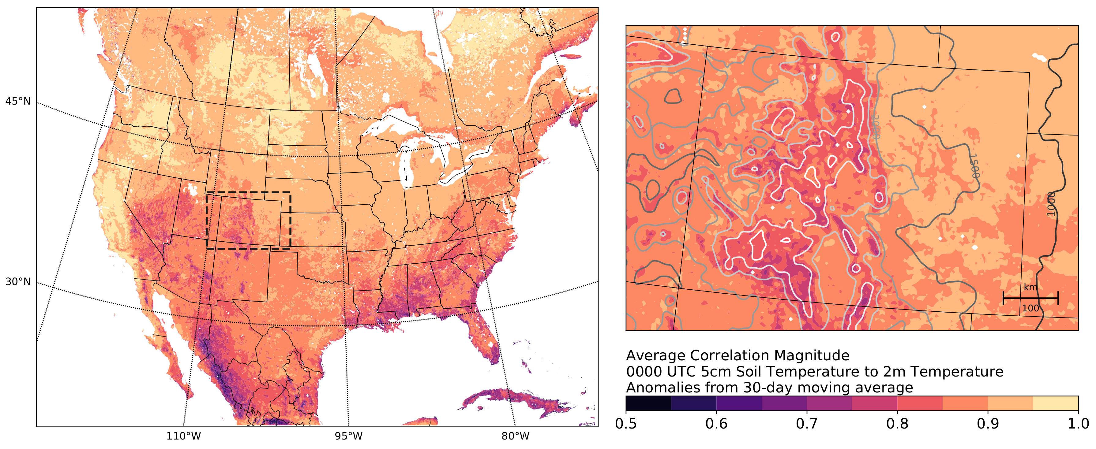
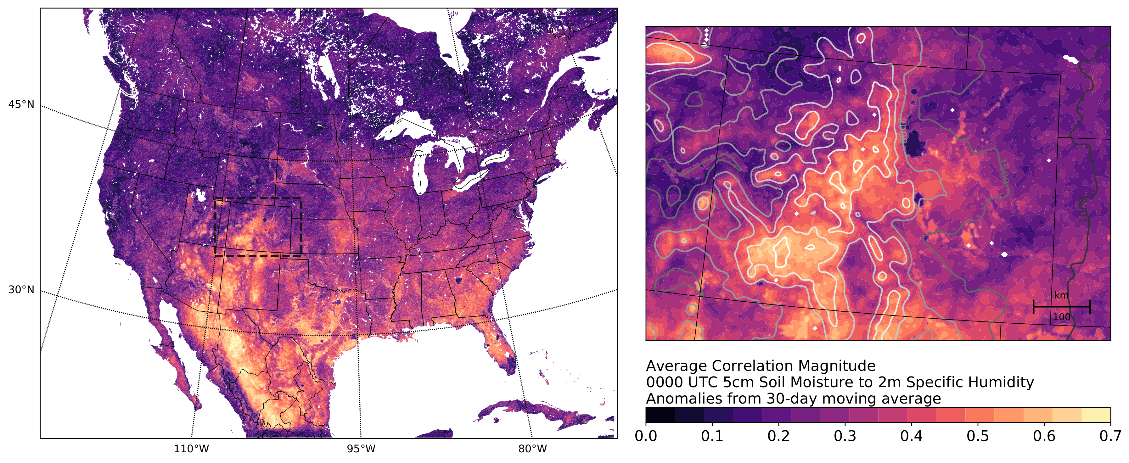
Figure 1 and
Figure 2 explore correlations between soil and 2-m air temperature and moisture in a long-running (13-year) high-resolution simulation of the current climate of North America [
48]. In brief, Liu et al. [
48] used the Weather Research and Forecasting (WRF) model to dynamically downscale the European Centre for Medium-Range Weather Forecasts (ECMWF) Reanalysis (ERA-Interim) atmospheric data to 4-km grid-spacing over North America over the historical period from 2000 to 2013. The initial and boundary conditions for the simulation are derived from the reanalysis, while local and convective scale features are allowed to freely evolve in the model.
Warm-season (July–September) 2-m air temperature, 5-cm soil temperature, 2-m specific humidity, and 5-cm volumetric soil water fraction at 0000 UTC each day are considered for a ten-year period from this simulation (2001–2010). For each year, temporal correlations between 2-m air temperature and 5-cm soil temperature (
Figure 1), and 2-m specific humidity and 5-cm volumetric soil water fraction (
Figure 2) anomalies from a 30-day moving average are computed at each grid point. The average correlation magnitudes are shown in these figures.
The correlations in
Figure 1 suggest that land and atmosphere may be less synchronized in the mountains than in flatter terrain. During the warm season the correlation between soil temperature and 2-m temperature is weaker in the mountains of North America compared with surrounding regions (
Figure 1). The high mountains in Colorado and California, and the other more mountainous regions of the western U.S. all show reduced correlation magnitudes. However, other factors also clearly influence the temperature coupling, such as local climate and vegetation. The latter appears to reduce the correlation magnitudes as well through the southeastern U.S. and the western slopes of the Sierra Madre range in Mexico, which are heavily vegetated but also have areas with complex terrain.
The coupling between soil moisture and the atmosphere is more complicated, with multiple drivers and both positive and negative feedbacks [
49]. Consequently, while the correlation between soil moisture and atmospheric moisture in the same model as above appears to have some correspondence with terrain, the relationship is not consistent (
Figure 2). For example, the highest mountains in Colorado, New Mexico, Arizona, and the Sierra Madre show high correlations, while other mountains such as the Sierras in California generally show lower correlations.
Figure 1 and
Figure 2 do illustrate the complexity and broad range of scales in lower boundary forcing that the mountains introduce. Compared with flatter terrain, the correlations vary spatially over much shorter distances. One can also expect that biases in both models and observations will also vary over short distances, and the horizontal correlations are similarly complex.
4.1. Methods for Enhancing Data Assimilation in Mountainous Environments
For the atmosphere, ensemble-based methods, including ensemble-variational hybrids that take advantage of instantaneous model states to estimate covariances, appear to be the most straightforward approach to dealing with the complex forcing imposed by the terrain. In mountainous environments, the error covariance estimated from an ensemble will include the effects of the modeled flow in the mountains. That is, they naturally include the effects of anisotropy in the terrain, and elevation differences as represented by the model. In contrast, variational methods require an
a priori specification of the error covariance matrix, which is difficult to adequately parameterize in mountainous terrain. Comparing an ensemble filter with a 3D-Var system using an isotropic background error covariance model shows this clearly [
29]. Additional anisotropic filtering helps the situation [
28], but cannot generalize when the scales of the terrain can change over short distances. Additional work on mitigating sampling error in ensemble-based systems is needed to take full advantage of the ensemble covariances in complex terrain.
The main challenge faced by land data assimilation in mountainous terrain is the increased surface heterogeneity. A promising approach to addressing this heterogeneity in a land/atmosphere data assimilation system would be to use an off-line (land-only) land data assimilation system, coupled to the atmospheric system. This approach would greatly reduce the cost of running the land model, making it affordable to use ensemble data assimilation (most appropriate for land data assimilation; [
51]). The land model could also be more easily run at higher resolution than the atmospheric model [
52]. Note that the resolution at which the land model and assimilation can be run will be limited by resolution of the available data sets of land characteristics (soil and vegetation type, land cover, topography). An off-line land data assimilation would be best set up by leveraging an existing on-line land data assimilation system coupled to an atmospheric system (e.g., [
53,
54]).
Coupled land–atmosphere data assimilation is challenging in any environment, due to uncertainties in modeling of the land/atmosphere exchanges, uncertainties in the modeling of the individual land and atmosphere components, and the scarcity of direct observations of the land surface. As outlined above, these modeling and observation issues are worse over mountainous terrain, making coupled assimilation even more challenging. While
Figure 1 and
Figure 2 suggest that land–atmosphere coupling may sometimes be weaker in mountainous terrain, the plotted correlations are still high (>0.6 across the Colorado Rockies in both Figures), indicating a strong potential to use coupled data assimilation to improve model forecasts of one component (say the atmosphere) by performing an assimilation update on the other component (say the land). Additionally,
Figure 1 and
Figure 2 relate only to warm-season conditions. During the cold seasons, snow cover has a strong impact on the simulated atmosphere, due to its insulative properties and dramatic effect on the surface albedo. The potential for atmospheric simulations to benefit from improved land data assimilation is also clear, using the strategies outlined above.
Examining the analysis increments from data assimilation can highlight systematic biases in the observations and/or models [
3,
28,
30]. This presents a choice of correcting the errors or interpreting them to improve the model. One consideration in making this choice is whether the model errors sufficiently degrade forecasts beyond the length of the assimilation cycle, which would suggest that the model climatology does not match what is observed. In this case, a more fruitful path to a robust predictive system may be to improve the model itself rather than rely on empirical bias adjustment.
Experimental output from land DA over mountainous terrain could also provide a tool to diagnose model errors, understand local flows in complex terrain, and assess the representativity of the atmospheric grid cell. For example, soil moisture in an integrator of precipitation inputs to the surface, and an off-line land assimilation that uses high-resolution observations (say from a field campaign) to constrain the model soil moisture could be used to infer details of the spatial distribution of precipitation at sub-atmospheric grid-scales (which are very difficult to observe confidently).
As noted in the previous discussions, accurately estimating observation bias is not easy, but improved observation bias estimation is an opportunity to improve analysis via data assimilation in the mountains. Good separation of model and observation bias remains a research topic. It stands to reason that data assimilation in the mountains can benefit disproportionately by pursuing it.
4.2. Opportunities from Field Programs for Exploring Data Assimilation in Mountainous Environments
An observation program could be constructed to obtain measurements aimed at improving models or observation systems within a data assimilation context. Because the data assimilation performance depends on details of both the observations and the models, the best observing program strategy may be different from one aimed solely at enhancing physical understanding. Thus, a data assimilation system, and one or more specific models, would be needed during all phases of a field campaign, from planning through execution and post-experiment analysis.
Field programs are most often designed to identify or better understand physical processes in the land, vegetation, or atmosphere. The data from the 1999 field campaign during the Mesoscale Alpine Programme (MAP) [
55] remains the richest observational data set for assimilation experiments in a mountainous environment. One of the key strengths of the MAP field campaign was its success in covering a wide range of spatial and temporal scales. Following that field campaign, several papers appeared that focused on mesoscale data assimilation, using systems and models that are now out of date [
56,
57,
58]. Revisiting those data with current models and assimilation systems with observing system experiments (OSEs) may identify immediately realizable gains from additional observational assets in and around the mountains.
Despite its strengths, the MAP project that focused on the planetary boundary layer did not emphasize assimilation as an outcome. The observations were limited to a cross section of a single valley, more specifically the Riviera section of the Ticino Valley in Switzerland. Similar boundary layer measurements were also taken in the Rhine valley. Both focused on atmospheric turbulence measurements, consistent with its goal of characterizing the boundary layer in a mountain-valley circulation. The measurements are problematic for data assimilation experiments because the areas (and therefore scales) they span are too small to measure any of the meaningful correlation length scales in current forecast models. Conversely, the Ticino and Rhine valleys are too far apart to expect robust correlations between the boundary layer structures that could be evaluated for utility in a data assimilation system.
The MAP boundary layer observations may be useful in more exploratory approaches that evaluate model error with the data assimilation system. Rather than simply comparing turbulence measurements to subgrid-scale parameterized turbulence, it is interesting to consider whether turbulence measurements can be assimilated into a fine-scale model with prognostic or diagnostic turbulent kinetic energy (TKE) equations that would provide a forward operator. This has not been attempted, and the nonlinear nature of TKE suggests that immediate success as measured by an improved forecasts may be hard to find. However, systematic departures of the TKE in a boundary layer that is reasonably well simulated would indicate flaws in the TKE treatment and possibly lead to model improvement. Rapid data assimilation cycling would be needed to keep the modeled boundary layer structurally similar to the observed one, and the work would build off of results such as those in Hacker and Angevine [
30], which focused on land–atmosphere exchanges in flat terrain.
Observations of the soil state are lacking in the MAP boundary layer-observing experiments, limiting exploration of the effects of the control of the surface on the atmosphere. In some respects the Mountain Terrain Atmospheric Modeling and Observations (MATERHORN) Program [
59] improved in that respect, but also lacked the large-scale components that MAP did include. A program combining the best of the MATERHORN and MAP campaigns for OSE and model error diagnosis would almost certainly lead to improved data assimilation and models for mountainous environments.
While remaining useful, designing field programs to improve models within a data assimilation context may require different decisions during the planning phases. Data assimilation can play a role in that planning, and also benefit from the outcomes. Prior to a field program, or the design of a long-term observation network, careful studies including the following can be informative: (1) high-resolution sensitivity studies, which are best performed in a data assimilation context [
60,
61]; (2) representativeness error diagnosis in observing-system simulation experiment (OSSE) and observing system experiment (OSE) contexts; and (3) linking observed scales to model scales. Results from those studies would help design a field program that addresses the key challenges in data assimilation described above.
The maturity of data assimilation systems today, and the computational power enabling fine-scale modeling, makes improved analysis and prediction in mountainous terrain more approachable than ever before. Through focused modeling and observation efforts, progress in data assimilation is possible. The complexity introduced by mountainous environments exposes many of the fundamental issues in data assimilation elsewhere, and consequently progress in the mountains immediately generalizes to other outstanding problems in modeling and data assimilation at fine scales.


